Dynamical thermalization of Bose-Einstein condensate
in Bunimovich stadium

Abstract

We study numerically the wavefunction evolution of a Bose-Einstein condensate in a Bunimovich stadium billiard being governed by the Gross-Pitaevskii equation. We show that for a moderate nonlinearity, above a certain threshold, there is emergence of dynamical thermalization which leads to the Bose-Einstein probability distribution over the linear eigenmodes of the stadium. This distribution is drastically different from the energy equipartition over oscillator degrees of freedom which would lead to the ultra-violet catastrophe. We argue that this interesting phenomenon can be studied in cold atom experiments.

Nonlinear dynamics and chaos Quantum chaos; semiclassical methods Bose-Einstein condensates in optical potentials

1 Introduction

Starting from the famous Fermi-Pasta-Ulam problem [1, 2] the interest to understanding of thermalization process in dynamical systems with a finite number of degrees of freedom is continuously growing (see e.g. [3, 4]). At present the experiments with cold Bose gas in atom traps and optical lattices open access to experimental investigations (see e.g. [5, 6]) stimulating the theoretical and experimental interest to this phenomenon (see e.g. [7, 8]).

The numerical analysis of dynamical thermalization in disordered nonlinear chains has been started recently showing that the quantum Gibbs distribution can appear at a moderate nonlinearity contrary to usually expected energy equipartition over linear modes [9, 10]. Thus it is interesting to analyze the dynamics of a Bose-Einstein condensate (BEC), described by the Gross-Pitaevskii Equation (GPE), in a chaotic billiard where the quantum evolution corresponds to a regime of quantum chaos and energy levels statistics described by the Random Matrix Theory [11, 12, 13]. As an example we use a de-symmetrized Bunimovich stadium where the classical dynamics is fully chaotic (see e.g. [14, 12]). We note that the chaotic optical billiards, created by a laser beam and containing cold atoms, have been already studied experimentally [15, 16] and hence our model can be investigated experimentally.

2 Model description

The model is described by the GPE for BEC in the de-symmetrized Bunimovich stadium billiard with Dirichlet boundary conditions:

$$i\hbar{\partial\psi(\vec{r},t)\over\partial t}=-{\hbar^{2}\over 2m}\Delta\psi(\vec{r},t)+\beta|\psi(\vec{r},t)|^{2}\psi(\vec{r},t)$$ (1)

where we consider $\hbar=1$, $m=0.5$. The height of the stadium is taken as $h=1$ and its maximal length is $l=2$ (see Fig. 1). Thus the average level spacing is $\Delta\approx 4\pi/A\approx 7.04$ where $A$ is the billiard area. At $\beta=0$ the numerical methods of quantum chaos allows to determine efficiently about million of eigenenergies of linear modes and related eigenmodes [17]. For comparison, we also consider the case on a rectangular billiard with approximately the same area as for stadium and with the golden mean ratio $l/h=(1+\sqrt{5})/2,h=1$. We note that for model (1) the spectrum of Bogoliubov excitations of BEC in a Bunimovich stadium had been studied in [18], but the question of dynamical thermalization has been not addressed there. We also point that the model (1) is described by the partial differential equation (continuous variables) thus being significantly more complex than the case of nonlinear chains studied in [9, 10]. Indeed, even the prove of the existence of solution in (1) is a nontrivial mathematical problem which still remains open (e.g. the ultra-violet catastrophe would imply the absence of solution). In the following we restrict our analysis to the GPE case not going beyond this description.

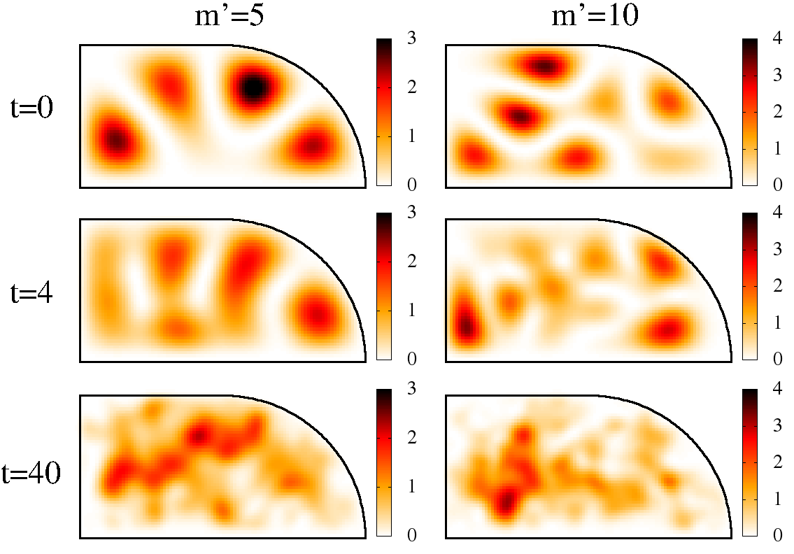
Figure 1: (Color on-line) Time evolution of wavefunction amplitude $|\psi(x,y,t)|$ in coordinate representation for an initial state of linear eigenstate mode $m^{\prime}=5$ (left column) and $m^{\prime}=10$ (right column) shown at $t=0$ (top panels). Middle and bottom panels show the snapshots of corresponding distributions at $t=4$ and $t=40$ respectively. Here $\beta=10$, color bars give values of $|\psi(x,y,t)|$.

The time evolution of (1) is integrated by small time steps of Trotter decomposition of linear and nonlinear terms with a step size going down to $\Delta t=4\times 10^{-5}$ to suppress nonlinear growth of high modes. We use $N_{c}=1076(1085)$ linear modes $\phi_{m}$ of stadium (rectangular) for linear part of time propagation doing the nonlinear step with $\beta$ term in the coordinate space with $N_{p}=11207(12816)$ points inside the billiard. The lattice points are given by $79\times 79=6241$ equidistant $x$-$y$ coordinates for the square part of the stadium billiard (rectangular billiard), and rays with equidistance in angles for the circular part. The change of basis from coordinates to energies (and viceversa) is given by a unitary matrix in double precision. Similar to [19], a special aliasing procedure is used with an efficient suppression of nonlinear numerical instability at high modes. This integration scheme exactly conserves the probability norm providing the total energy conservation with an accuracy better than $2\%$ at largest value $\beta=20$ and better than $1\%$ at lower $\beta$ values. At any step the wavefunction is expanded in the basis of linear modes $\phi_{m}$ so that $\psi(x,y,t)=\sum_{m}C_{m}(t)\phi_{m}(x,y)$. The averaging of probabilities $w_{m}(t)=|C_{m}(t)|^{2}$ ($\sum_{m}w_{m}=1$) over time gives the average probability distribution $\rho_{m}=\langle|C_{m}|^{2}\rangle_{t}$.

We note that the quantum evolution of GPE (1) has been studied in the frame of quantum turbulence for a rectangular billiard [20] and for a 3D-cube [21]. However, in these studies there is energy injection/absorption at low/high modes to generate the Kolmogorov energy flow in space of linear modes (see e.g. [22, 23]). We also note that the time evolution of wave packet for the GPE in Bunimovich stadium had been simulated in [24] but only a spacial distribution had been considered there. In contrast to these studies we consider only unitary or Hamiltonian evolution given by (1) being interested in the distribution properties of probabilities $\rho_{m}$ over linear eigenmodes. In this respect our approach is different from other studies where the analysis had been concentrated on space fluctuations (see e.g. [25]). Also, as we will see below, there is a significant difference for the GPE evolution in chaotic and rectangular billiards.

3 Time evolution

Examples of time evolution for two initial eigenmodes $m^{\prime}=5,10$ are shown in Fig. 1 at $\beta=10$ (video is available at [26]). They show that, due to nonlinearity inside the stadium, there are complex irregular oscillations of wavefunction with time.

Another representation is obtained by considering the time evolution of probabilities $w_{m}(t)$ in the basis of linear modes shown in Fig. 2. At moderate value $\beta=2$ the probability remains located only in a few modes without thermalization and spreading over many modes. For larger value of $\beta=10$ the nonlinear spearing over modes goes in a more efficient way with many excited modes. Thus the dynamical thermalization is expected to be absent at small or moderate $\beta<\beta_{c}\sim 1$ while for large nonlinearities $\beta\sim 10>\beta_{c}$ we may expect the emergence of dynamical thermalization.

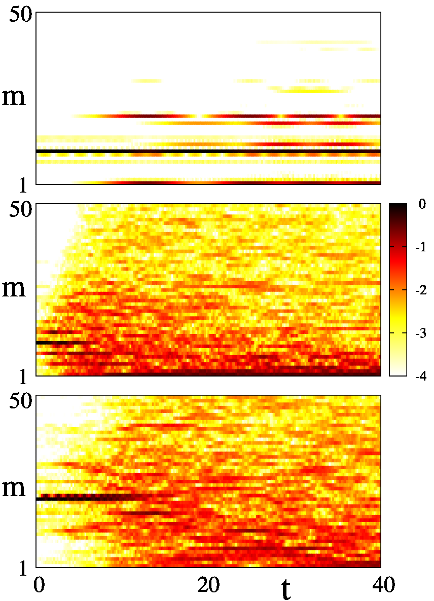
Figure 2: (Color on-line) Time evolution of probabilities $w_{m}(t)$ in linear mode basis for initial state $m^{\prime}=10$ at $\beta=2$ (top panel), $m^{\prime}=10,20$ at $\beta=10$ (middle and bottom panels respectively). The probabilities $w_{m}(t)$ are averaged over time interval $\delta t=0.2$ to reduce fluctuations; color bar shows values of $\log_{10}\rho_{m}(m^{\prime})$.

For the initial state $m^{\prime}=10$ we have the approximate energy value $E_{m}\approx m^{\prime}\Delta\approx mv^{2}/2\approx 70$, where $v\approx\sqrt{280}$ is a velocity of classical particle and a time interval between collisions is approximately $\tau_{col}\approx h/v\approx 0.06$. Thus during the time $t=40$ we have approximately $N_{col}=t/\tau_{col}\approx 670$. Dynamical thermalization is reasonably achieved for time interval $t\in[20,40]$ as it is visible in middle and bottom panels of Fig.2 where $w_{m}(t)$ have thermalized like distribution with $\beta=10$.

4 Bose-Einstein thermal distribution

To characterize the dynamical thermalization in more detail we assume that a moderate nonlinearity acts as a certain thermalizer which drives the system to a thermal equilibrium over quantum levels of the stadium. At the same time we assume that the nonlinear term is not very strong so that it does not affect significantly the average linear eigenenergies. Indeed, on average we have $\beta|\psi|^{2}\approx\beta/A\approx\Delta$ for $\beta\sim 10$, so that indeed, the nonlinear energy shift is moderate at such values of $\beta$.

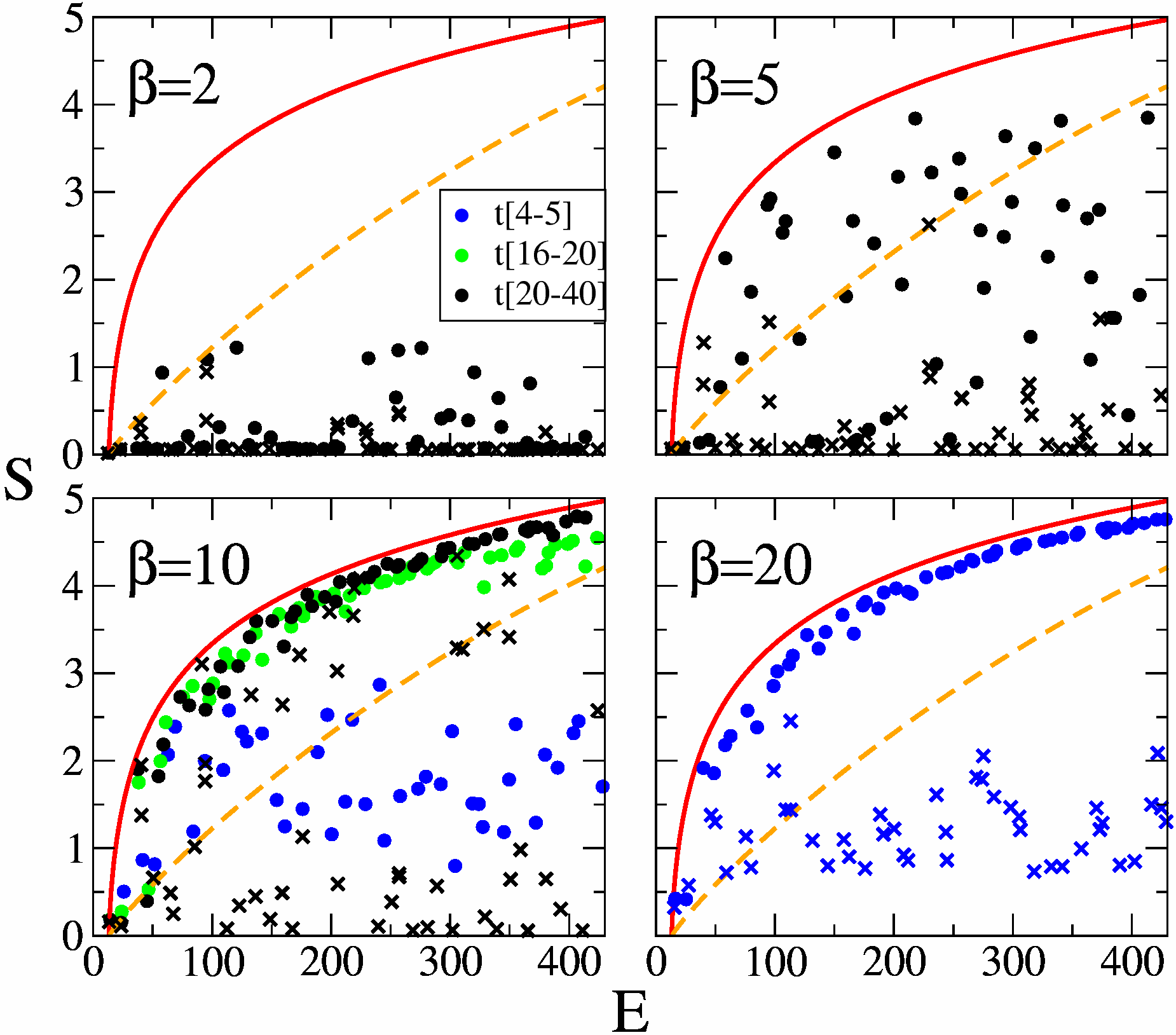
Figure 3: (Color on-line) Entropy dependence on energy $S(E)$ obtained from the GPE time evolution of initial linear eigenstates with $1\leq m^{\prime}\leq 50$ for the stadium (circles) and rectangular (crosses) billiards for nonlinearity $\beta=2,5,10,20$ marked on each panel. Here the average is done over time intervals $t\in[4,5]$ (blue), $t\in[16,20]$ (green) and $t\in[20,40]$ (black). The red curve represents the Bose-Einstein ansatz (2) while the orange dashed curve shows the case of energy equipartition over first 50 modes of the stadium.

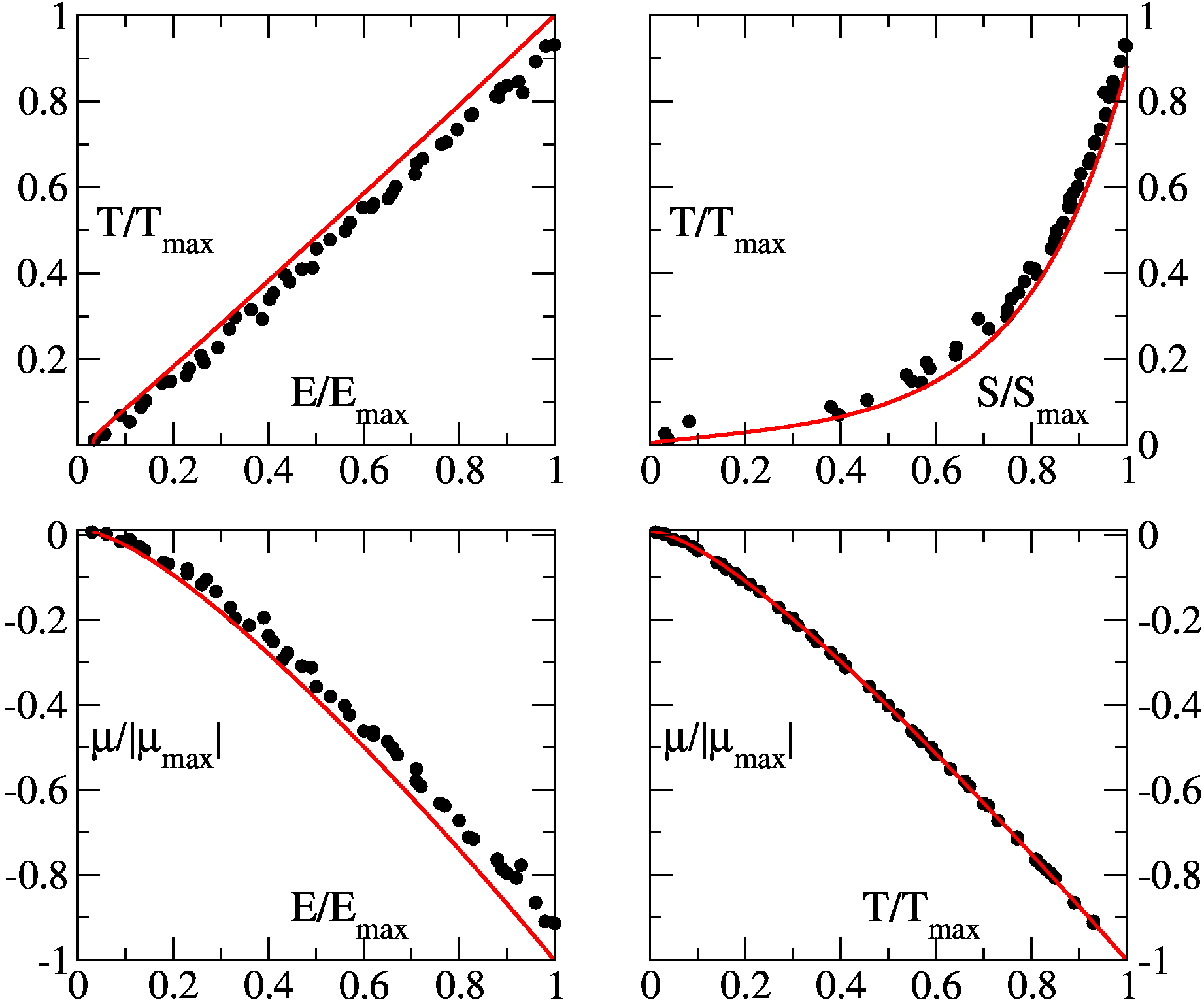
Figure 4: (Color on-line) Theoretical dependencies given by Bose-Einstein ansatz (2) and shown by the red curves for $T(E)$ (top left panel), $T(S)$ (top right panel), $\mu(E)$ (bottom left panel), $\mu(T)$ (bottom right panel); the numerical results, obtained from GPE in the stadium, are shown by black points at $\beta=10$ with averaging over the time interval $[20,40]$. For representation convenience we show these dependencies using rescaling to maximal values of variables corresponding to initial state with $m^{\prime}=50$: $E_{max}=414$, $S_{max}=4.8$, $T_{max}=387.75$, $|\mu_{max}|=1500.45$.

Thus we expect that nonlinearity generates a dynamical thermalization over the quantum billiard energy levels. In such a case we should have the standard Bose-Einstein distribution ansatz over energy levels $E_{m}$ [27]:

$$\rho_{m}=1/[\exp[(E_{m}-E_{g}-\mu)/T]-1]$$ (2)

where $E_{g}=13.25$ is the energy of the ground state, $T$ is the temperature of the system, $\mu(T)$ is the chemical potential dependent on temperature. The values $E_{m}$ are the eigenenergies of the stadium at $\beta=0$. The parameters $T$ and $\mu$ are determined by the norm conservation $\sum_{m=1}^{\infty}\rho_{m}=1$ (we have only one particle in the system) and the initial energy $\sum_{m}E_{m}\rho_{m}=E$. The entropy $S$ of the system is determined by the usual relation [27]: $S=-\sum_{m}\rho_{m}\ln\rho_{m}$. The relation (2) with normalization condition determines the implicit dependencies on temperature $E(T)$, $S(T)$, $\mu(T)$.

The advantage of energy $E$ and entropy $S$ is that both are extensive variables, thus they are self-averaging and due to that they have reduced fluctuations. Due to this feature $S$ and $E$ are especially convenient for verification of the thermalization ansatz. To check this ansatz we start from an initial linear mode $m^{\prime}$ which corresponds to the system energy $E\approx E_{m^{\prime}}$ and follow the GPE time evolution of probabilities $w_{m}(t)$ determining the value of entropy $S$ from obtained average probabilities $\rho_{m}$. Considering the initial states with $1\leq m^{\prime}\leq 50$ we obtain the numerical dependence $S(E)$ shown by symbols in Fig. 3. This dependence is compared with the analytic curve following from the Bose-Einstein ansatz (2) which gives the dependencies $E(T)$ and $S(T)$ and hence provides the analytic dependence $S(E)$ shown by the red curve in Fig. 3.

The data of Fig. 3 show that even at large $\beta=20$ there is no thermalization for the rectangular billiard. We attribute this to the fact that the ray dynamics is integrable in this billiard and thus it is much more difficult to reach onset of chaos for the GPE in this billiard at moderate nonlinearity studied here.

The situation is different for the stadium: at $\beta=2$ only a few modes are populated, at $\beta=5$ the number of modes is increased but still the numerical data for $S$ are very far from the thermalization red curve (at least on the time scale reached in our numerical simulations). However, for $\beta=10,20$ we find that the numerical data at large times $t>15$ follow the theoretical curve $S(E)$ given by the Bose-Einstein thermalization. A small visible deviation from theory is still visible since the numerical points are systematically slightly below the theory curve. We attribute this to a finite computation time which apparently is not long enough to visit all regions of multi-configurational space with sufficiently large statistics. On the basis of obtained data we can conclude that the dynamical thermalization in the stadium sets in for $\beta>\beta_{c}\approx 7\approx\Delta$. We also checked that the initial states, which represent a linear combination of a few eigenmodes, also follow the theoretical red curve in Fig. 3 at $\beta>\beta_{c}$ (e.g. two modes $m=10,15$ at $\beta=10$).

Another way to check the thermalization predictions is to determine $T$ from the numerical values of $E$, $S$ which, according to the Bose-Einstein ansatz, give independent values $T_{1}(E)$ and $T_{2}(S)$. The average value $T=(T_{1}+T_{2})/2$ is shown in Fig. 4 as a function of numerical values of $E$ and $S$. We see that the numerical points are in a good agreement with the analytic curves (apart of small systematic displacement of numerical points discussed in the paragraph above). In a similar way we make a comparison between the theory and numerical data for dependencies $\mu(E)$ and $\mu(T)$ shown in bottom panels of Fig. 3. Again we find a good agreement between the numerical data and the Bose-Einstein thermalization distribution (2).

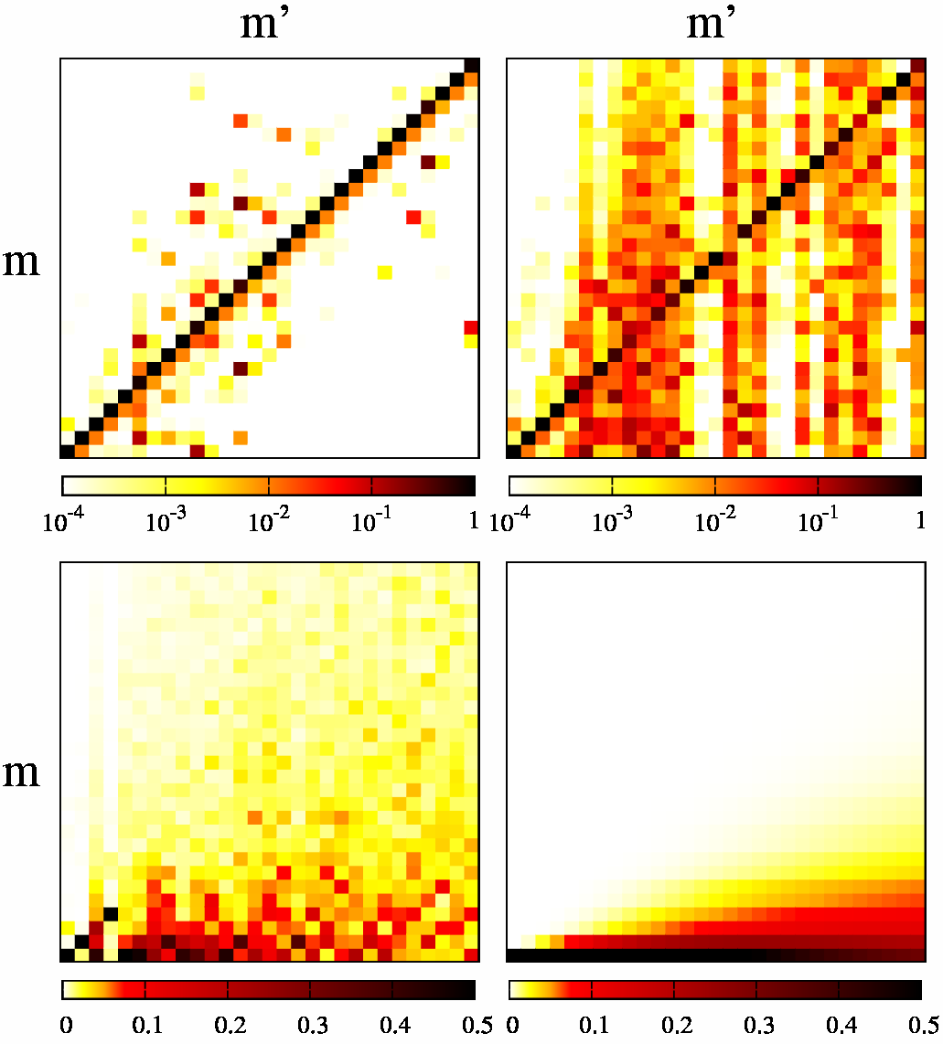
Figure 5: (Color on-line) Time averaged probabilities $\rho_{m}(m^{\prime})$ at stadium eigenstate $m$ for initial state $m^{\prime}$; the time averaging is done for time intervals $[20,40]$; the panels show data for $1\leq m^{\prime},m\leq 30$ in $x,y$ axes respectively. Here we show the cases: $\beta=2$ (top left panel), $\beta=5$ (top right panel), $\beta=10$ (bottom left panel), the theoretical Bose-Einstein distribution (2) (bottom right panel). The values of $\rho_{m}(m^{\prime})$ are shown by color with the corresponding color bars for each panel.

The validity of the Bose-Einstein thermalization ansatz (2) leads to a striking paradox pointed already for nonlinear chains in [10]: formally the GPE in stadium gives a system of equations for nonlinear coupled oscillators (we have nonlinear coupling between linear oscillator modes of the stadium) with a moderate nonlinearity. The usual expectations of the statistical mechanics predict the energy equipartition between these modes [27, 10]. If the number of modes is infinite then we should have ultra-violet catastrophe with probabilities $\rho_{m}\sim 1/E_{m}$ at high modes $m$ and the global temperature approaching zero as $T\sim 1/m_{max}$ for initial excitation with $m^{\prime}\sim 10$ (here $m_{max}$ is the maximal mode number). This classical thermalization ansatz for $m_{max}=50$ is shown by a dashed curve in Fig. 3 and the data clearly show that it is very different from the numerical data which are close to the Bose-Einstein ansatz (we note that numerically the quantum Gibbs distribution [10] over quantum levels of stadium gives the results being rather close to those of (2) since at low temperatures and large $m$ values both distributions are rather similar). Thus our data clearly show the emergence of the dynamical thermalization described by the Bose-Einstein distribution in a chaotic billiard for moderate nonlinearity $\beta>\beta_{c}\sim\Delta$.

A more detailed check of the Bose-Einstein distribution requires a direct comparison of numerically obtained probabilities $\rho_{m}(m^{\prime})$ with the theoretical expression (2) for each initially excited mode $m^{\prime}$. We show such data in Fig. 5 for $\beta=2,5,10$. It is clear that there is no thermalization at $\beta=2,5$ since a large fraction of probability remains at the initially populated state $m=m^{\prime}$. For $\beta=10$ we see that the probability at initial state $m^{\prime}$ drops significantly indicating emergence of dynamical thermalization. However, still the numerical probabilities at large $m$ have larger values compared to those of the theory (2) shown in the bottom right panel of Fig. 5. We attribute this to the fact that our total computation time is not large enough to have good statistical data for average values of $\rho_{m}(m^{\prime})$ which require good averaging and long computation times. Such a problem had been visible in the numerical simulations with nonlinear chains [9, 10] where the time of simulations have been by a few orders of magnitude larger than here. At the same time the extensive property of energy $E$ and entropy $S$ makes them self-averaging and more stable in respect to fluctuations thus allowing to compare them with the theory (2) at significantly shorter time scales.

Unfortunately the large scale simulations of the GPE for stadium are rather heavy and time consuming since they require transformations from coordinate to linear mode space and small integration time step with aliasing procedure to suppress numerical instabilities of high modes. It is possible that the numerical codes can be improved allowing to reach larger time scales but this requires further studies going beyond the scope of this work.

Finally we discuss a preparation of one or a few initial eigenstates considered above for the time evolution and dynamical thermalization. It is clear that the ground state of the billiard is relatively easy to prepare since it is the final state in a process of relaxation and also since it is compact in space being close to a coherent state of a harmonic trap. An excited state can be produced from the ground state applying a monochromatic driving (oscillation) of the billiard that creates an effective ac-potential $V_{ac}=fx\cos(\omega t)$ if one goes to the oscillating frame (see e.g. [28]). In a chaotic billiard dipole matrix elements have transitions between all energy eigenstates [28] and thus a resonant transition will populate one or a few states being close to the resonance $E_{n}\approx E_{0}+\hbar\omega$. We note that such a method demonstrated already its efficiency for excitation of high energy states for chaotic Rydberg atoms (see e.g. [29, 30]).

5 Discussion

Our studies of the GPE in the Bunimovich stadium billiard show that for a moderate nonlineariy parameter above a certain threshold $\beta>\beta_{c}\approx\Delta$ the nonlinear Hamiltonian dynamics leads to emergence of dynamical thermalization over the linear billiard modes which is well described by the Bose-Einstein distribution. This distribution is strikingly different from the usually expected energy equipartition over modes [27, 10] which would lead to a violet catastrophe with a significant probability transfer to higher and higher modes of the chaotic billiard. The established validity of the Bose-Einstein distribution, together with the previous studies of dynamical thermalization in nonlinear chains [9, 10], leads to an unexpected conclusion about emergence of quantum distributions over linear energy modes in systems of coupled nonlinear oscillators at moderate nonlinearity. This result is drastically different from the standard energy equipartition picture expected for nonlinear dynamics of oscillator systems [1, 2, 3, 4, 27].

The described picture of “quantum” dynamical thermalization for the GPE in chaotic billiards requires a better understanding of nonlinear dynamics in systems with many degrees of freedom. It is known that slow chaos, like the Arnold diffusion [31, 32, 33], and an anomalous diffusion in disordered nonlinear chains (see e.g. [19, 34, 35, 36]) generate a number of features which still wait their deep understanding. We hope that our results will stimulate further research in this field of fundamental aspects of nonlinear dynamics and thermalization onset in systems with large but finite number of degrees of freedom.

The modern progress in the cold atom experiments allows to investigate a dynamics of Bose gas and Bose-Einstein condensates [5, 6] while the chaotic billiard for such atoms can be created by optical beams [15, 16]. Thus we think that the model (1) can be realized with cold atom experiments.

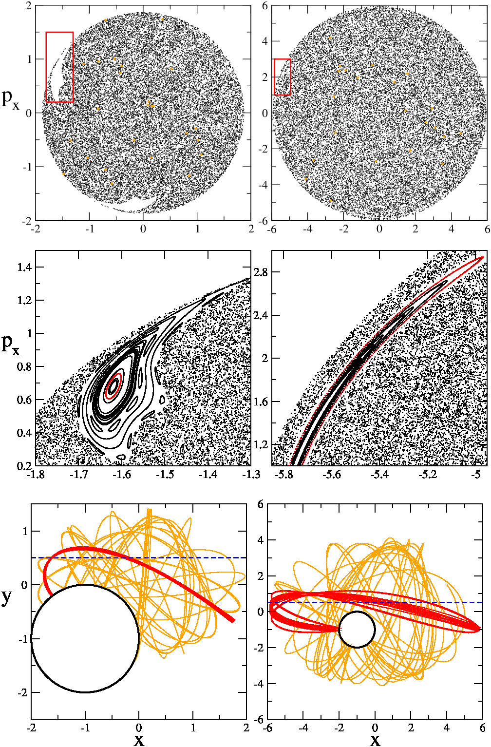
Figure 6: (Color on-line) Poincaré sections $(x,p_{x})$ at $y=0.5,p_{y}>0$. Left and right columns correspond to energy $E=2$ and $E=18$ respectively. Top panels show the entire Poincaré sections (10 chaotic orbit up to time $t\leq 10^{4}$) and middle panels show zoom marked in top panels (adding 15 trajectories in the integrable region to time $t\leq 10^{4}$), one invariant curve of each panel is highlighted with red (gray) color inside stability island at middle panels. Bottom panels show dynamics in $(x,y)$ plane with stable orbits from middle panels (same red color) and chaotic orbits (orange color also shown in top panels) up to times $t=10^{2}$; dashed horizontal lines mark $y=0.5$ used for the Poincaré sections.

Another promising possibility can be an experimental realization of a harmonic Sinai billiard, or Sinai oscillator. An example of such a billiard is described by a classical Hamiltonian $H=({p_{x}}^{2}+x^{2})/2+({p_{y}}^{2}+2y^{2})/2$ with a rigid disk of radius $r_{d}=1$ located at $x=y=-1$ (thus the ratio of frequencies in $x$ and $y$ is irrational). The harmonic potential can be realized by optical traps while the repulsive rigid disk can be created inside by an additional laser beam with such a frequency detuning that it acts as a repulsive potential for cold atoms. Examples of typical trajectories in such a billiard are shown in Fig. 6. In the same figure we also show the Poincaré sections constructed in $(x,p_{x})$ plane at $y=0.5,\;p_{y}>0$ with energies $E=2$ and $E=18$, when the size of oscillations of atom is larger than $r_{d}$. In this regime almost all phase space is chaotic (the domains of integrable dynamics are very small). Thus we think that the GPE in such a harmonic Sinai billiard will show all the effects of dynamical thermalization discussed above for a more convential case of the Bunimovich stadium. We expect that such a system can be more simple for experimental investigations. Also in such a billiard a coherent state of the harmonic potential can be created experimentally and can be used as an initial state with energy being close to the energies of linear eigenmodes of such a billiard. We expect that experimental investigations of the GPE in a harmonic Sinai billiard (or in the Bunimovich stadium) will allow to understand the fundamental aspects of dynamical thermalization.

We thank D.Guéry-Odelin for useful discussions of cold atom physics.

References

- [1] \NameFermi E., Pasta J., Ulam S. and Tsingou M. \BookLos Alamos Report No.LA-1940 (unpublished) \Year1955
- [2] \NameFermi E. \BookCollected papers vol.2 \PublUniversity of Chicago Press,Chicago \Year1965
- [3] \NameCampbell D.K., Rosenau P. and Zaslavsky G. (eds.) \BookA focus issue on “The Fermi-Pasta-Ulam problem - The First 50 Years” \REVIEWChaos15(1)20051
- [4] \Name Gallavotti G (ed.) \BookThe Fermi-Pasta-Ulam problem \PublSpringer Lect. Notes in Physics v.738, Berlin \Year2008
- [5] \NameTrotzky S. et al. \REVIEWNature Phys.82012325.
- [6] \NameLangen T. et al. \REVIEWScience3482015207.
- [7] \NameSinatra A., Lobo C. and Castin Y. \REVIEWPhys. Rev. Lett.872001210404.
- [8] \NameCarusotto I. and Castin Y. \REVIEWC.R. Physique52004107.
- [9] \NameMulansky M., Ahnert K., Pikovsky A. and Shepelyansky D.L. \REVIEWPhys. Rev. E802009056212.
- [10] \NameErmann L. and Shepelyansky D.L. \REVIEWNew J. Phys.152013123004.
- [11] \NameBohigas O., Giannoni M.J. and Schmit C. \REVIEWPhys. Rev. Lett.5119841.
- [12] \NameStöckmann H.-J. \BookQuantum chaos: an introduction \PublCambridge Univ. Press, Cambridge \Year1999
- [13] \NameHaake F. \BookQuantum signatures of chaos \PublSpringer, Berlin \Year2010
- [14] \NameBunimovich L. \REVIEWScholarpedia2(8)20071813.
- [15] \NameMilner V., Hanssen J.L., Campbell W.C. and Raizen M.G. \REVIEWPhys. Rev. Lett.8620011514.
- [16] \NameFriedman N., Kaplan A., Carasso D. and Davidson N. \REVIEWPhys. Rev. Lett.8620011518.
- [17] \NameVergini E. and Saraceno M. \REVIEWPhys. Rev. E5219952204.
- [18] \NameZhang C., Liu J., Raizen M.G. and Niu Qian. \REVIEWPhys. Rev. Lett.932004074101.
- [19] \NameShepelyansky D.L. \REVIEWEur. Phys. J. B852012199.
- [20] \NamePromet D., Nazarenko S. and Onorato M. \REVIEWPhys. Rev. A802009056103(R).
- [21] \NameFujimoto K. and Tsubota M. \PublarXiv:1502.03274 [cond-mat.quant-gas] \Year2015
- [22] \NameZakharov V.E., L’vov V.S. and Falkovich G. \Book Kolmogorov spectra of turbulence \PublSpringer-Verlag, Berlin \Year1992
- [23] \NameNazarenko S. \BookWave turbulence \PublSpringer-Verlag, Berlin \Year2011
- [24] \NameXiong H. and Wu B. \REVIEWPhys. Rev. A822010053634.
- [25] \NameXiong H.W. and Wu B. \REVIEWLaser Phys. Lett.82011398.
- [26] \NameErmann L and Shepelyansky D.L. \Publhttp/www.quantware.ups-tlse.fr/QWLIB/becstadium/ Accessed May (2015)
- [27] \NameLandau L.D. and Lifshitz E.M. \BookStatistical mechanics \PublWiley, New York \Year1976
- [28] \NameProsen T. and Shepelyansky D.L. \REVIEWEur. Phys. J. B462005515.
- [29] \NameIu Chun-ho., Welch G.R., Kash M.M., Kleppner D., Delande D. and Gay J.C. \REVIEWPhys. Rev. Lett.661991145.
- [30] \NameKoch P.M. and van Leeuwen K.A.H. \REVIEWPhys. Reports2551995289.
- [31] \NameChirikov B.V. \REVIEWPhys. Reports521979263.
- [32] \NameChirikov B.V. and Vecheslavov V.V. \REVIEWSov. Phys. JETP85(3)1997616 \PublZh. Eksp. Teor. Fiz. 112 (1997) 1132
- [33] \NameMulansky M., Ahnert K., Pikovsky A. and Shepelyansky D.L. \REVIEWJ. Stat. Phys.14520111256.
- [34] \NamePikovsky A.S. and Shepelyansky D.L. \REVIEWPhys. Rev. Lett.1002008094101.
- [35] \NameFishman S., Krivolapov Y. and Soffer A. \REVIEWNonlinearity2220002861.
- [36] \NameLaptyeva T.V., Ivanchenko M.V. and Flach S. \REVIEWJ. Phys. A: Math. Theor.472014493001.