Unifying inflation with late-time acceleration by a BIonic system

Abstract

We propose a cosmological model that unifies inflation, deceleration and acceleration phases of expansion history by a BIonic system. At the beginning, there are $k$ black fundamental strings that transited to the BIon configuration at a given corresponding point. Here, two coupled universes, brane and antibrane, are created interacting each other through a wormhole and inflate. With decreasing temperature, the energy of this wormhole flows into the universe branes and lead to inflation. After a short time, the wormhole evaporates, the inflation ends and a deceleration epoch starts. By approaching the brane and antibrane universes together, a tachyon is born, grows and causes the creation of a new wormhole. At this time, the brane and antibrane universes result connected again and the late-time acceleration era of the universe begins. We compare our model with previous unified phantom models and observational data obtaining some cosmological parameters like temperature in terms of time. We also find that deceleration parameter is negative during inflation and late-time acceleration epochs, while it is positive during the deceleration era. This means that the model is consistent, in principle, with cosmological observations.

I Introduction

Recent observations coming from supernovae surveys, large scale structure and cosmic microwave background radiation show that the Universe is presently undergoing a phase of accelerated phantom expansion q1 ; q2 . Before this era, expansion was decelerated, at least up to the nucleosynthesis time. This stage of universe history is well explained by the non-phantom type cosmic fluids. However, another period of accelerated expansion, named inflation, acts at very early epochs describing expansion in agreement with observational data q3 ; q4 ; q5 ; q6 ; q7 . Up to now, several models have been presented to unify the early time inflation with the today observed accelerated phantom phase. For example, some authors have found that the Universe dynamics begins by an inflationary phase and converges towards a $\Lambda$CDM model if the fluid coupled to dark energy has a negative energy density at early time q8 . Other authors have considered the recent cosmological deceleration-acceleration transition redshift in $f(R)$ gravity. They proposed a model where the deceleration parameter changes sign at a redshift consistent with observations q9 . In other scenarios, the future evolution of quintessence/phantom dominated epoch in modified $f(R)$ gravity has been considered odirev ; noi . This type of gravity unifies the early-time inflation with late-time acceleration and is consistent, in principle, with observational data q10 . Furthermore the universe expansion history, unifying early-time inflation and late-time acceleration, can be realized in scalar-tensor gravity minimally or non-minimally coupled to curvature q11 .

However, one of the best models unifying the early-time inflation with late-time acceleration is the phantom cosmology. This model allows to study the inflationary epoch, the transition to the non-phantom standard cosmology (radiation/matter dominated eras) and today observed dark energy epoch. In the unified phantom cosmology, the same scalar field plays the role of early time (phantom) inflaton and late-time Dark Energy. The recent transition from decelerating to accelerating phase can be also described by the same scalar field q12 . Despite of this reliable features, the main question that arises is on the origin of the phantom field. The answer to this question can come, at a fundamental level, by taking into account a brane-antibrane system undergoing three different stages along its evolution. At first stage, $k$ black fundamental strings transit to the so called BIon configuration at matching point. The BIon is a configuration in flat space of a brane universe and a parallel anti-brane universe connected by a wormhole q13 ; q14 . At transition point, the thermodynamics of this configuration can be matched to that of $k$ non-extremal black fundamental strings. At lower temperature, the wormhole throat becomes smaller, its energy is transferred to the universe branes and leads to its accelerated expansion. After a short time, this wormhole evaporates, inflation ends and non-phantom era begins. This is the second stage of Universe expansion history. Eventually, two brane and antibrane universes become close to each other, the tachyonic potential between them increases and a new wormhole is formed. At this stage, the Universe evolves from the non-phantom phase to the phantom one and consequently, the late phantom-dominated era starts and ends up in the big-rip singularity.

We can compare this dynamics with the results in Ref. q12 and obtain the wormhole throat features and temperature in terms of time.

The outline of the paper is the following. In Sec. II, we discuss the inflationary stage in BIon system and show that all cosmological parameters depend on the wormhole parameters between the two branes. In Sec. III, we study the second stage where the wormhole evaporates and the pair brane and antibrane universes result disconnected. In Sec. IV, we consider the third stage where a new tachyonic wormhole is formed between branes and accelerates the destruction of the universes towards a big rip. In Sec. V, we test our model against observational data. The last section is devoted to summary and conclusions.

II Stage 1: The early time inflation

In this section, we assume that there is only a fluid of $k$ black fundamental strings at the beginning. In our model, the Universe is born at a point corresponding where the thermodynamics of $k$ non-extremal black fundamental strings is matched to that of the BIon configuration. We will construct the inflation in BIon and discuss that the wormholes between branes have direct effect on the inflation. We can also show that all parameters of inflation depend on the number of branes and on the distance between branes.

Let us start with the supergravity solution for $k$ coincident non-extremal black $F$-strings lying along the $z$ direction as discussed in q14 ; q15 :

$$ds^{2}=H^{-1}(-fdt^{2}+dz^{2})+f^{-1}dr^{2}+r^{2}d\Omega_{7}^{2},$$

$$H=1+\frac{r_{0}^{6}\sinh^{2}\bar{\alpha}}{r^{6}},\>f=1-\frac{r_{0}^{6}}{r^{6}},$$

$$\>k^{2}=\frac{3^{12}T_{D3}^{4}(\cosh^{2}\bar{\alpha}-1)}{2^{12}\pi^{6}T_{F1}^{2}T^{12}\cosh^{10}\bar{\alpha}}.$$ (1)

In above equation, $T$ is the finite temperature of BIon, $k$ is the number of black $F$-strings and $T_{D_{3}}$ and $T_{F1}$ are tensions of brane and fundamental strings respectively. The mass density along the $z$ direction can be found from the metric q15 :

$$\frac{dM_{F1}}{dz}=T_{F1}k+\frac{16(T_{F1}k\pi)^{3/2}T^{3}}{81T_{D3}}+\frac{40T_{F1}^{2}k^{2}\pi^{3}T^{6}}{729T_{D3}^{2}}.$$ (2)

At the corresponding point, the $k$ black $F$-strings transit to the BIon configuration where the string coupling constant ($g_{s}\ll 1$) becomes very small. On the other hand, brane tension depends on the inverse of string coupling (${\displaystyle T_{D3}=\frac{1}{(2\pi)^{3}g_{s}l_{s}^{4}}})$ and tends to larger values at transition point. However, the string tension (${\displaystyle T_{F1}=\frac{1}{2\pi l_{s}^{2}}}$) remains constant and thus ${\displaystyle\frac{40T_{F1}^{2}k^{2}\pi^{3}T^{6}}{729T_{D3}^{2}}=\frac{840g_{s}^{2}l_{s}^{4}k^{2}\pi^{7}T^{6}}{729}}$ is smaller than ${\displaystyle\frac{16(T_{F1}k\pi)^{3/2}T^{3}}{81T_{D3}}=\frac{16g_{s}l_{s}\pi^{3}(2k)^{3/2}T^{3}}{81}}$ and both are smaller than 1. Finally, we can write:

$$\frac{dM_{F1}}{dz}=T_{F1}k+AT^{3}+BT^{6}$$

$$A=\frac{16(T_{F1}k\pi)^{3/2}}{81T_{D3}}=\frac{16g_{s}l_{s}\pi^{3}(2k)^{3/2}}{81}\ll 1$$

$$B=\frac{40T_{F1}^{2}k^{2}\pi^{3}}{729T_{D3}^{2}}=\frac{840g_{s}^{2}l_{s}^{4}k^{2}\pi^{7}}{729}\ll 1$$

$$\frac{B}{A}\simeq g_{s}l_{s}^{4}\ll 1$$ (3)

Thus, we can ignore higher orders of (${\displaystyle\frac{1}{T_{D3}}}$) in our calculations but the above approximation is valid. For finite temperature BIon configurations, the metric takes the form q14 :

$$ds^{2}=-dt^{2}+dr^{2}+r^{2}(d\theta^{2}+\sin^{2}\theta d\phi^{2})+\sum_{i=1}^{6}dx_{i}^{2}.$$ (4)

If one chooses the world volume coordinates of the $D3$-brane as $\{\sigma^{a},a=0..3\}$ and defining $\tau=\sigma^{0},\,\sigma=\sigma^{1}$, then, the coordinates of BIon assume the form q13 ; q14 :

$$t(\sigma^{a})=\tau,\,r(\sigma^{a})=\sigma,\,x_{1}(\sigma^{a})=z(\sigma),\,\theta(\sigma^{a})=\sigma^{2},\,\phi(\sigma^{a})=\sigma^{3}$$ (5)

and the remaining coordinates $x_{i=2,..6}$ are constant. The embedding function $z(\sigma)$ describes the bending of the brane. Let $z$ be a transverse coordinate to the branes and $\sigma$ be the radius on the world-volume. The induced metric on the brane is:

$$\gamma_{ab}d\sigma^{a}d\sigma^{b}=-d\tau^{2}+(1+z^{\prime}(\sigma)^{2})d\sigma^{2}+\sigma^{2}(d\theta^{2}+\sin^{2}\theta d\phi^{2})$$ (6)

so that the spatial volume element is ${\displaystyle dV_{3}=\sqrt{1+z^{\prime}(\sigma)^{2}}\sigma^{2}d\Omega_{2}}$. We impose the two boundary conditions $z(\sigma)\rightarrow 0$ for $\sigma\rightarrow\infty$ and $z^{\prime}(\sigma)\rightarrow-\infty$ for $\sigma\rightarrow\sigma_{0}$, where $\sigma_{0}$ is the minimal two-sphere radius of the configuration. For this BIon, the mass density along the $z$ direction can be obtained q14 :

$$\frac{dM_{BIon}}{dz}=T_{F1}k+\frac{3\pi T_{F1}^{2}k^{2}T^{4}}{32T_{D3}^{2}\sigma_{0}^{2}}+\frac{7\pi^{2}T_{F1}^{3}k^{3}T^{8}}{512T_{D3}^{4}\sigma_{0}^{4}}.$$ (7)

As it can be seen from the above equation, the mass density along the $z$ direction depends on the brane tension ($T_{D3}$). At transition point, a brane and an antibrane are produced and expand very fast. Consequently, $T_{D3}$ grows and achieve large values. On the hand, the string tension (${\displaystyle T_{F1}=\frac{1}{2\pi l_{s}^{2}}}$) remains constant and thus ${\displaystyle\frac{7\pi^{2}T_{F1}^{3}k^{3}T^{8}}{512T_{D3}^{4}\sigma_{0}^{4}}}$ is smaller than ${\displaystyle\frac{3\pi T_{F1}^{2}k^{2}T^{4}}{32T_{D3}^{2}\sigma_{0}^{2}}}$ and both are smaller than 1. It is

$$\frac{dM_{BIon}}{dz}=T_{F1}k+A^{\prime}T^{4}+B^{\prime}T^{8}$$

$$A^{\prime}=\frac{3\pi T_{F1}^{2}k^{2}}{32T_{D3}^{2}\sigma_{0}^{2}}=\frac{48\pi^{5}g_{s}^{2}l_{s}^{2}k^{2}}{32\sigma_{0}^{2}}\ll 1$$

$$B^{\prime}=\frac{7\pi^{2}T_{F1}^{3}k^{3}}{512T_{D3}^{4}\sigma_{0}^{4}}=\frac{7\pi^{11}g_{s}^{4}l_{s}^{10}k^{3}}{\sigma_{0}^{4}}\ll 1$$

$$\frac{B^{\prime}}{A^{\prime}}\simeq\frac{1}{T_{D3}^{2}}\simeq g_{s}^{2}l_{s}^{8}\ll 1$$ (8)

For this reason, we can ignore higher order terms in this expression. Comparing the mass densities for BIon to the mass density for the $F$-strings, we see that the thermal BIon configuration behaves like $k$ $F$-strings at $\sigma=\sigma_{0}$. At this corresponding point, $\sigma_{0}$ should have the following dependence on the temperature:

$$\sigma_{0}=\left(\frac{\sqrt{kT_{F1}}}{T_{D3}}\right)^{1/2}\sqrt{T}\left[C_{0}+C_{1}\frac{\sqrt{kT_{F1}}}{T_{D3}}T^{3}\right].$$ (9)

where $T_{F1}=4k\pi^{2}T_{D3}g_{s}l_{s}^{2}$, $C_{0}$, $C_{1}$, $F_{0}$, $F_{1}$ and $F_{2}$ are numerical coefficients which can be determined by requiring that the $T^{3}$ and $T^{6}$ terms in Eqs. (2) and (7) are matched. At this point, the two universes are born while the wormhole is not formed yet. The metric of these Friedman-Robertson-Walker (FRW) universes are:

$$ds^{2}_{Uni1}=ds^{2}_{Uni2}=-dt^{2}+a(t)^{2}(dx^{2}+dy^{2}+dz^{2}).$$ (10)

The mass density of black $F$-string, BIon and two universes have to be equal at the corresponding point:

$$\rho_{uni1}+\rho_{uni2}=\frac{dM_{F1}}{dz}=\frac{dM_{BIon}}{dz}\rightarrow$$

$$-6H^{2}=T_{F1}k+\frac{16(T_{F1}k\pi)^{3/2}T^{3}}{81T_{D3}}+\frac{40T_{F1}^{2}k^{2}\pi^{3}T^{6}}{729T_{D3}^{2}},$$ (11)

where $H$ is the Hubble parameter. Solving this equation, we obtain:

$$a(T)=a(0)e^{-X(T)},$$

$$X(T)=\frac{1}{\sqrt{6}}\left(T_{F1}k+\frac{16(T_{F1}k\pi)^{3/2}T^{3}}{81T_{D3}}+\frac{40T_{F1}^{2}k^{2}\pi^{3}T^{6}}{729T_{D3}^{2}}\right)^{1/2}.$$ (12)

At the beginning, we have $T=\infty$ that decreases with time. On the other hand, Eq. (12) shows that, at this time, the scale factor is zero and with the decreasing of temperature, the Universe expands.

After a short period, the wormhole is formed between brane and antibrane due to the $F$-string charge and the Universe is entering the inflationary phase. Assuming $k$ units for the $F$-string charge along the radial direction and using Eq. (6), we obtain q13 ; q14 :

$$z(\sigma)=\int_{\sigma}^{\infty}d\acute{\sigma}(\frac{F(\acute{\sigma})^{2}}{F(\sigma_{0})^{2}}-1)^{-\frac{1}{2}}.$$ (13)

At finite temperature BIon configuration, the $F(\sigma)$ is given by

$$F(\sigma)=\sigma^{2}\frac{4\cosh^{2}\alpha-3}{\cosh^{4}\alpha},$$ (14)

where $\cosh{\alpha}$ is determined by the following function:

$$\cosh^{2}\alpha=\frac{3}{2}\frac{\cos\frac{\delta}{3}+\sqrt{3}\sin\frac{\delta}{3}}{\cos\delta},$$ (15)

with the definitions:

$$\cos{\delta}\equiv\overline{T}^{4}\sqrt{1+\frac{k^{2}}{\sigma^{4}}},\quad\overline{T}\equiv\left(\frac{9\pi^{2}N}{4\sqrt{3}T_{D_{3}}}\right)T,\quad\kappa\equiv\frac{kT_{F1}}{4\pi T_{D_{3}}}$$ (16)

In the last equation, $T$ is the finite temperature of the BIon system, $N$ is the number of $D3$-branes, $T_{D_{3}}$ and $T_{F1}$ are the tensions of branes and fundamental strings respectively. Attaching a mirror solution to Eq. (13), we construct the wormhole configuration. The estimation of separation distance $\Delta=2z(\sigma_{0})$ between the $N$ $D3$-branes and $N$ anti-$D3$-branes for a given brane-antibrane wormhole configuration depends on the four parameters $N$, $k$, $T$ and $\sigma_{0}$. We have:

$$\Delta=2z(\sigma_{0})=2\int_{\sigma_{0}}^{\infty}d\acute{\sigma}\left(\frac{F(\acute{\sigma})^{2}}{F(\sigma_{0})^{2}}-1\right)^{-\frac{1}{2}}.$$ (17)

In in the limit of small temperatures, we obtain:

$$\Delta=\frac{2\sqrt{\pi}\Gamma(5/4)}{\Gamma(3/4)}\sigma_{0}\left(1+\frac{8}{27}\frac{k^{2}}{\sigma_{0}^{4}}\overline{T}^{8}\right).$$ (18)

Let us now discuss the non-phantom inflationary model of universe in the thermal BIon system. In order to discuss this scenario, we have to compute the contribution of the BIonic system to the four-dimensional energy-momentum tensor. The energy-momentum tensor for a BIonic system with $N$ $D3$-branes and $k$ $F$-string charges is q14 ,

$$T^{00}=\frac{2T_{D3}^{2}}{\pi T^{4}}\frac{F(\sigma)}{\sqrt{F^{2}(\sigma)-F^{2}(\sigma_{0})}}\sigma^{2}\frac{4\cosh^{2}\alpha+1}{\cosh^{4}\alpha}$$

$$T^{ii}=-\gamma^{ii}\frac{8T_{D3}^{2}}{\pi T^{4}}\frac{F(\sigma)}{\sqrt{F^{2}(\sigma)-F^{2}(\sigma_{0})}}\sigma^{2}\frac{1}{\cosh^{2}\alpha},\,i=1,2,3$$

$$T^{44}=\frac{2T_{D3}^{2}}{\pi T^{4}}\frac{F(\sigma)}{F(\sigma_{0})}\sigma^{2}\frac{4\cosh^{2}\alpha+1}{\cosh^{4}\alpha}$$ (19)

We assume this higher-dimensional stress-energy tensor to be a perfect fluid of the form ($T_{i}^{j}={\mathop{\rm diag}\nolimits}\left[{-\rho,p,p,p,\bar{p},p,p,p}\right])$ where $\bar{p}$ is the pressure in the extra space-like dimension. In above the equation, we allow the pressure in the extra dimension to be different with respect to the pressure in the $3D$ space. Therefore, this stress-energy tensor expresses a homogeneous, anisotropic perfect fluid in ten dimensions. This equation shows that with increasing temperature in BIonic system, the energy-momentum tensors decreases. This is because that when spikes of branes and antibranes are well separated, wormhole is not formed and there is no channel for flowing energy from universe branes into extra dimensions. This means that temperature is very high. However when the two universe branes are close to each other and connected by a wormhole, temperature reduces to lower values.

Now, we can discuss the phantom cosmological model in finite temperature BIon configuration and obtain the explicit form of temperature and equation of state parameter $\omega$. To this end, we use the approach reported in Ref. q12 in order to unify BIonic and phantom inflation through the three phases of universe expansion.

A phantom cosmological model can be described by the following action:

$$S=\int d^{4}x\sqrt{-g}\{\frac{1}{2k^{2}}R-\frac{1}{2}\omega(\phi)\partial_{\mu}\phi\partial^{\mu}\phi-V(\phi)\}$$ (20)

Here, $\omega(\phi)$ and $V(\phi)$ are functions of the scalar field $\phi$. The energy density $\rho$ and the pressure $p$ are:

$$\rho=\frac{1}{2}\omega(\phi)\dot{\phi}^{2}+V(\phi),$$

$$p=\frac{1}{2}\omega(\phi)\dot{\phi}^{2}-V(\phi).$$ (21)

Furthermore, the FRW cosmological equations are given by q12 :

$$\rho_{uni1}=\rho_{uni2}=\frac{3}{k^{2}}H^{2},$$

$$p_{uni1}=p_{uni2}=-\frac{1}{k^{2}}(3H^{2}+2\dot{H})$$

$$\rho_{tot}=2\rho_{uni1},p_{tot}=2p_{uni1}.$$ (22)

Using these FRW equations, the effective equation of state is:

$$\omega_{eff}=\frac{p_{tot}}{\rho_{tot}}=-1-\frac{2}{3}\frac{\dot{H}}{H^{2}}.$$ (23)

Now, the scalar field $\phi$, the Hubble rate H and the scale factor $a(t)$ can be chosen follow as:

$$\phi=t,$$

$$H=h_{0}^{2}\left(\frac{1}{t_{0}^{2}-\phi^{2}}+\frac{1}{t_{1}^{2}+\phi^{2}}\right),$$

$$a(t)=a_{0}\left(\frac{t+t_{0}}{t_{0}-t}\right)^{\frac{h_{0}^{2}}{2t_{0}}}e^{-\frac{h_{0}^{2}}{2t_{0}}Arctan(\frac{t_{1}}{t})}.$$ (24)

Then, using Eqs. (23) and (24), the effective EoS parameter is written as q11 ; q12 :

$$\omega_{eff}=\frac{p}{\rho}=-1-\frac{8}{3h_{0}^{2}}\frac{t(t-t_{+})(t-t_{-})}{(t_{1}^{2}+t_{0}^{2})^{2}}$$ (25)

Since a = 0 at $t=-t_{0}$, one may regard this time corresponding to the birth of the universe. We find that $H$ has two minima at $t=t_{\pm}=\pm\sqrt{\frac{t_{0}^{2}-t_{1}^{2}}{2}}$ and at $t=0$. Besides $H$ has a local maximum. Hence, the phantom phase ($\omega_{eff}<-1$) occurs for $t_{-}<t<0$ and $t>t_{+}$, while the non-phantom phase ($\omega_{eff}>-1$) for $-t_{0}<t<t_{-}$ and $0<t<t_{+}$. It is worth noticing that there is a Big Rip type singularity at t = $t_{0}$ q11 ; q12 .

Now, using Eq. (19), we obtain the equation of state on the universe brane in the finite temperature BIon configuration:

$$\omega_{BIon}=-\frac{4\cosh^{2}\alpha}{4\cosh^{2}\alpha+1}\left(1+\frac{(t_{-})^{2}-(t-t_{-})^{2}}{(t-t_{-})^{2}}\right).$$ (26)

As it can been seen from Eq. (26), the equation of state is less than -1 in the range of $t_{-}<t<0$ and it is evaluated from phantom to non-phantom phase at $t=0$. Equating this equation of state with equation of state in Eq. (25) , we can find the explicit form of temperature $T$, that is

$$T\sim\left(1+\frac{(t_{-})^{2}-(t-t_{-})^{2}}{(t-t_{-})^{2}}\right)^{1/4}\frac{1}{\left(1+\frac{8}{3h_{0}^{2}}\frac{t(t-t_{+})(t-t_{-})}{(t_{1}^{2}+t_{0}^{2})^{2}}\right)}.$$ (27)

Eq. (27) indicates that temperature is infinite at $t=t_{-}$ and decreases with time. However, the velocity of this decreasing is very high in the range of $t_{-}<t<0$. This result is in good agreement with observational data.

We assume that the wormhole is created at $t=t_{-}$ and $\sigma=\sigma_{0}$ and it vanishes at $t=0$ and $\sigma_{0}=0$. In this period of time, we can write: $\sigma_{0}=\frac{0-t}{0-t_{-}}\sigma$. Using this and putting the energy density of the two universes equal to the energy density of the BIon, we obtain $\sigma$ in terms of time:

$$\rho_{tot}=\rho_{BIon}\rightarrow\frac{6}{k^{2}}H^{2}=\frac{2T_{D3}^{2}}{\pi T^{4}}\frac{F(\sigma)}{\sqrt{F^{2}(\sigma)-F^{2}(\sigma_{0})}}\sigma^{2}\frac{4\cosh^{2}\alpha+1}{\cosh^{4}\alpha}\rightarrow$$

$$\sigma\sim\left(1+\frac{(t_{-})^{2}-(t-t_{-})^{2}}{(t-t_{-})^{2}}\right)^{-1/4}\left(\frac{(t-t_{-})}{(t_{-})^{2}-(t-t_{-})^{2}}\right)\left(1+\frac{8}{3h_{0}^{2}}\frac{t(t-t_{+})(t-t_{-})}{(t_{1}^{2}+t_{0}^{2})^{2}}\right)$$ (28)

According to this result, $\sigma$ is zero at $t=t_{-}$; however, with time evolution, it accelerates and tends to very higher values in a short period. From this point of view, the behavior of $\sigma$ is the same as the scale factor $a(t)$.

III Stage 2: The non-phantom standard cosmology

In this section, we propose a model that allows to consider the non-phantom model in the brane-antibrane system. In this stage, with decreasing temperature and distance between two branes, the wormhole between brane and anti-brane evaporates and tachyon is born. The expansion of the two FRW universes is controlled by the tachyonic potential between branes and evolves from non-phantom to phantom phase.

To construct a non-phantom model, we consider a set of $D3$-$\overline{D3}$-brane pairs in the background (6) which are placed at points $z_{1}=l/2$ and $z_{2}=-l/2$ respectively so that the separation between the brane and antibrane is $l$. For the simple case of a single $D3$-$\overline{D3}$-brane pair with open string tachyon, the action is q16 :

$$S=-\tau_{3}\int d^{9}\sigma\sum_{i=1}^{2}V(TA,l)e^{-\phi}(\sqrt{-detA_{i}})$$

$$(A_{i})_{ab}=\left(g_{MN}-\frac{TA^{2}l^{2}}{Q}g_{Mz}g_{zN}\right)\partial_{a}x^{M}_{i}\partial_{b}x^{M}_{i}+F^{i}_{ab}+\frac{1}{2Q}((D_{a}TA)(D_{b}TA)^{\ast}+(D_{a}TA)^{\ast}(D_{b}TA))$$

$$+il(g_{az}+\partial_{a}z_{i}g_{zz})(TA(D_{b}TA)^{\ast}-TA^{\ast}(D_{b}TA))+il(TA(D_{a}TA)^{\ast}-TA^{\ast}(D_{a}TA))(g_{bz}+\partial_{b}z_{i}g_{zz}),$$ (29)

where

$$Q=1+TA^{2}l^{2}g_{zz},$$

$$D_{a}TA=\partial_{a}TA-i(A_{2,a}-A_{1,a})TA,V(TA,l)=g_{s}V(TA)\sqrt{Q},$$

$$e^{\phi}=g_{s}(1+\frac{R^{4}}{z^{4}})^{-\frac{1}{2}},$$ (30)

The quantities $\phi$, $A_{2,a}$ and $F^{i}_{ab}$ are the dilaton field, the gauge fields and field strengths on the world-volume of the non-BPS brane respectively; $TA$ is the tachyon field, $\tau_{3}$ is the brane tension and $V(TA)$ is the tachyon potential. The indices $a,b$ denote the tangent directions of $D$-branes, while the indices $M,N$ run over the background ten-dimensional space-time directions. The $Dp$-brane and the anti-$Dp$-brane are labeled by $i$ = 1 and 2 respectively. Then the separation between these $D$-branes is defined by $z_{2}-z_{1}=l$. Also, in writing the above action, we are using the convention $2\pi\acute{\alpha}=1$.

Let us consider, for simplicity, the only $\sigma$ dependence of the tachyon field $TA$ and set the gauge fields to zero. In this case, the action (29) in the region that $r>R$ and $TA^{\prime}\sim constant$ simplifies to

$$S\simeq-\frac{\tau_{3}}{g_{s}}\int dt\int d\sigma\sigma^{2}V(TA)(\sqrt{D_{1,TA}}+\sqrt{D_{2,TA}}),$$ (31)

where $D_{1,TA}=D_{2,TA}\equiv D_{TA}$, ${\displaystyle V_{3}=\frac{4\pi^{2}}{3}}$ is the volume of a unit sphere $S^{3}$ and

$$D_{TA}=1+\frac{l^{\prime}(\sigma)^{2}}{4}+TA^{2}l^{2},$$ (32)

where the prime denotes a derivative with respect to $\sigma$. A useful potential that can be used is q17 ; q18 ; q19 :

$$V(TA)=\frac{\tau_{3}}{\cosh\sqrt{\pi}TA}.$$ (33)

The energy momentum tensor is obtained from the action by calculating its functional derivative with respect to the ten-dimensional background metric $g_{MN}$. The variation is ${\displaystyle T^{MN}=\frac{2}{\sqrt{-detg}}\frac{\delta S}{\delta g_{MN}}}$. We get q16 ,

$$T^{00}_{i}=V(TA)\sqrt{D_{TA}},$$

$$T^{zz}_{i}=-V(TA)\frac{1}{\sqrt{D_{TA}}}(TA^{2}l^{2}+\frac{\acute{l}^{2}}{4})$$

$$T^{\sigma\sigma}_{i}=-V(TA)\frac{Q}{\sqrt{D_{TA}}}$$ (34)

Now, using the above equation, we obtain the equation of state as:

$$\omega_{brane-antibrane}=-\frac{1+TA^{2}l^{2}}{1+\frac{l^{\prime 2}}{4}+TA^{2}l^{2}}$$ (35)

This equation indicates that the equation of state is negative both at the beginning and at the end of this era and bigger than -1 in the range of $0<t<t_{+}$. Assuming the equation of state equal to the equation of state in (25) (which corresponds to the unified theory and can be applied for all the three phases) and assuming $\sigma\sim t$, $l\sim l_{0}(1-\frac{t_{+}t^{2}}{2}+\frac{t^{3}}{3})$ and $l^{\prime}\sim l_{0}t(t-t_{+})$ , we get:

$$TA\sim\frac{t^{4}}{(t_{1}^{2}+t_{0}^{2})\left(2+\frac{8}{3h_{0}^{2}}\frac{t(t_{+}-t)(t-t_{-})}{(t_{1}^{2}+t_{0}^{2})^{2}}\right)}$$ (36)

Eq. (36 ) shows that when two branes are very distant from each other (t=0, $l=l_{0}$), the tachyon field is zero , whereas moving the branes towards each other, the value of tachyon increases and becomes very large at $t=t_{+}$.

IV Stage 3: The late-time acceleration

In the previous section, we considered that the tachyon field grows slowly ($TA\sim t^{4}/t^{3}=t$) and we ignored ${\displaystyle TA^{\prime}=\frac{\partial TA}{\partial\sigma}}$ and ${\displaystyle\dot{TA}=\frac{\partial TA}{\partial t}}$ in our calculations. In this section, we discuss that with the decreasing of the distance separation between the brane and antibrane universes, the tachyon field grows very fast and $TA^{\prime}$ and $\dot{TA}$ cannot be discarded. This dynamics leads to the formation of a new wormhole. In this stage, the Universe evolves from non-phantom phase to a new phantom phase and consequently, the phantom-dominated era of the universe accelerates and ends up into the Big-Rip singularity. In this case, the action (29) is given by the following Lagrangian $L$:

$$L\simeq-\frac{\tau_{3}}{g_{s}}\int d\sigma\sigma^{2}V(TA)(\sqrt{D_{1,TA}}+\sqrt{D_{2,TA}}),$$ (37)

where

$$D_{1,TA}=D_{2,TA}\equiv D_{TA}=1+\frac{l^{\prime}(\sigma)^{2}}{4}+\dot{TA}^{2}-TA^{\prime 2},$$ (38)

where we assume that $TAl\ll TA^{\prime}$. Now, we study the Hamiltonian corresponding to the above Lagrangian. In order to derive such Hamiltonian, we need the canonical momentum density ${\displaystyle\Pi=\frac{\partial L}{\partial\dot{TA}}}$ associated with the tachyon, that is

$$\Pi=\frac{V(TA)\dot{TA}}{\sqrt{1+\frac{l^{\prime}(\sigma)^{2}}{4}+\dot{TA}^{2}-TA^{\prime 2}}},$$ (39)

so that the Hamiltonian can be obtained as:

$$H_{DBI}=4\pi\int d\sigma\sigma^{2}\Pi\dot{TA}-L.$$ (40)

By choosing $\dot{TA}=2TA^{\prime}$, this gives:

$$H_{DBI}=4\pi\int d\sigma\sigma^{2}\left[\Pi(\dot{TA}-\frac{1}{2}TA^{\prime})\right]+\frac{1}{2}TA\partial_{\sigma}(\Pi\sigma^{2})-L$$ (41)

In this equation, we have, in the second step, integrated by parts the term proportional to $\dot{TA}$, indicating that tachyon can be studied as a Lagrange multiplier imposing the constraint $\partial_{\sigma}(\Pi\sigma^{2}V(TA))=0$ on the canonical momentum. Solving this equation yields:

$$\Pi=\frac{\beta}{4\pi\sigma^{2}},$$ (42)

where $\beta$ is a constant. Using (42) in (40), we get:

$$H_{DBI}=\int d\sigma V(TA)\sqrt{1+\frac{l^{\prime}(\sigma)^{2}}{4}+\dot{TA}^{2}-TA^{\prime 2}}F_{DBI},$$

$$F_{DBI}=\sigma^{2}\sqrt{1+\frac{\beta}{\sigma^{2}}}$$ (43)

The resulting equation of motion for $l(\sigma)$, calculating by varying (43), is

$$\left(\frac{l^{\prime}F_{DBI}}{4\sqrt{1+\frac{l^{\prime}(\sigma)^{2}}{4}}}\right)^{\prime}=0$$ (44)

Solving this equation, we obtain:

$$l(\sigma)=4\int_{\sigma}^{\infty}d\sigma\left(\frac{F_{DBI}(\sigma)}{F_{DBI}(\sigma_{0})}-1\right)^{-\frac{1}{2}}=4\int_{\sigma}^{\infty}d\sigma^{\prime}\left(\frac{\sqrt{\sigma_{0}^{4}+\beta^{2}}}{\sqrt{\sigma^{\prime 4}-\sigma_{0}^{4}}}\right)$$ (45)

This solution, for non-zero $\sigma_{0}$, represents a wormhole with a finite size throat. However, this solution is not complete, because we ignored the acceleration of branes. This acceleration is due to the tachyon potential between the branes ( ${\displaystyle a\sim\frac{\partial V(T)}{\partial\sigma}}$). According to recent investigations q20 , each of the accelerated branes and antibranes detects the Unruh temperature(${\displaystyle T=\frac{\hbar a}{2k_{B}\pi c}}$). We will show that this system is equivalent to the black brane. The equation of motion obtained from action (43) is:

$$\left(\frac{1}{\sqrt{D_{TA}}}TA^{\prime}(\sigma)\right)^{\prime}=\frac{1}{\sqrt{D_{TA}}}\left[\frac{V^{\prime}(TA)}{V(TA)}(D_{TA}-TA^{\prime}(\sigma)^{2})\right]$$ (46)

We can reobtain this equation in accelerated fame from the equation of motion in the flat background of (6):

$$-\frac{\partial^{2}TA}{\partial\tau^{2}}+\frac{\partial^{2}TA}{\partial\sigma^{2}}=0$$ (47)

By using the following re-parameterizations

$$\rho=\frac{\sigma^{2}}{w},$$

$$w=\frac{V(TA)\sqrt{D_{TA}}F_{DBI}}{2M_{D3-brane}}$$

$$\bar{\tau}=\gamma\int_{0}^{t}d\tau^{\prime}\frac{w}{\dot{w}}-\gamma\frac{\sigma^{2}}{2}$$ (48)

and doing following calculations:

$$\left\{\left[\left(\frac{\partial\bar{\tau}}{\partial\tau}\right)^{2}-\left(\frac{\partial\bar{\tau}}{\partial\sigma}\right)^{2}\right]\frac{\partial^{2}}{\partial\tau^{2}}+\left[\left(\frac{\partial\rho}{\partial\sigma}\right)^{2}-\left(\frac{\partial\rho}{\partial\tau}\right)^{2}\right]\frac{\partial^{2}}{\partial\rho^{2}}\right\}TA=0$$ (49)

we have:

$$(-g)^{-1/2}\frac{\partial}{\partial x_{\mu}}\left[(-g)^{1/2}g^{\mu\nu}\right]\frac{\partial}{\partial x_{\upsilon}}TA=0$$ (50)

where $x_{0}=\bar{\tau}$, $x_{1}=\rho$ and the metric elements are obtained as:

$$g^{\bar{\tau}\bar{\tau}}\sim-\frac{1}{\beta^{2}}\left(\frac{w^{\prime}}{w}\right)^{2}\frac{\left(1-\left(\frac{w}{w^{\prime}}\right)^{2}\frac{1}{\sigma^{4}}\right)}{\left(1+\left(\frac{w}{w^{\prime}}\right)^{2}\frac{(1+\gamma^{-2})}{\sigma^{4}}\right)^{1/2}}$$

$$g^{\rho\rho}\sim-(g^{\bar{\tau}\bar{\tau}})^{-1}$$ (51)

where we have used of previous assumption($\frac{\partial TA}{\partial t}=\frac{\partial TA}{\partial\tau}=2\frac{\partial TA}{\partial\sigma}$).

Now, we can compare these elements with the line elements of one black $D3$-brane q21 :

$$ds^{2}=D^{-1/2}\bar{H}^{-1/2}(-fdt^{2}+dx_{1}^{2})+D^{1/2}\bar{H}^{-1/2}(dx_{2}^{2}+dx_{3}^{2})+D^{-1/2}\bar{H}^{1/2}(f^{-1}dr^{2}+r^{2}d\Omega_{5})^{2},$$

(52)

where

$$f=1-\frac{r_{0}^{4}}{r^{4}},$$

$$\bar{H}=1+\frac{r_{0}^{4}}{r^{4}}\sinh^{2}\alpha,$$

$$D^{-1}=\cos^{2}\varepsilon+H^{-1}\sin^{2}\varepsilon,$$

$$\cos\varepsilon=\frac{1}{\sqrt{1+\frac{\beta^{2}}{\sigma^{4}}}}.$$ (53)

Eqs. (51) and (52) lead to

$$f=1-\frac{r_{0}^{4}}{r^{4}}\sim 1-\left(\frac{w}{w^{\prime}}\right)^{2}\frac{1}{\sigma^{4}},$$

$$\bar{H}=1+\frac{r_{0}^{4}}{r^{4}}\sinh^{2}\alpha\sim 1+\left(\frac{w}{w^{\prime}}\right)^{2}\frac{(1+\gamma^{-2})}{\sigma^{4}}$$

$$D^{-1}=\cos^{2}\varepsilon+\bar{H}^{-1}sin^{2}\varepsilon\simeq 1$$

$$\Rightarrow r\sim\sigma,r_{0}\sim\left(\frac{w}{w^{\prime}}\right)^{1/2},(1+\gamma^{-2})\sim\sinh^{2}\alpha$$ (54)

The temperature of the BIon system is ${\displaystyle T=\frac{1}{\pi r_{0}\cosh\alpha}}$ q13 . Consequently, the temperature of the brane-antibrane system can be calculated as:

$$T=\frac{1}{\pi r_{0}\cosh\alpha}=\frac{\gamma}{\pi}\left(\frac{w^{\prime}}{w}\right)^{1/2}\sim$$

$$\frac{\gamma}{\pi}\left(\tanh\sqrt{\pi}TA+\frac{l^{\prime}l^{\prime\prime}+TA^{\prime}TA^{\prime\prime}}{1+\frac{l^{\prime}(\sigma)^{2}}{4}+TA^{\prime 2}}+\frac{\frac{\beta}{\sigma^{3}}}{1+\frac{\beta}{\sigma^{2}}}\right)$$ (55)

However, this result should be corrected. Because $\gamma$ depends on the temperature and we can write:

$$\gamma=\frac{1}{\cosh\alpha}\sim\frac{2\cos\delta}{3\sqrt{3}-\cos\delta-\frac{\sqrt{3}}{6}\cos^{2}\delta}\sim$$

$$\frac{2\bar{T}^{4}\sqrt{1+\frac{\beta^{2}}{\sigma^{4}}}}{3\sqrt{3}-\bar{T}^{4}\sqrt{1+\frac{\beta^{2}}{\sigma^{4}}}-\frac{\sqrt{3}}{6}\bar{T}^{8}(1+\frac{\beta^{2}}{\sigma^{4}})}$$ (56)

Using Eqs. (55) and (56), we can approximate the explicit form of temperature:

$$T\sim\left(\frac{4\sqrt{3}T_{D_{3}}}{9\pi^{2}N}\right)\frac{\sqrt[3]{\pi}}{\sqrt[6]{1+\frac{\beta^{2}}{\sigma^{4}}}}\left(\tanh\sqrt{\pi}TA+\frac{l^{\prime}l^{\prime\prime}+TA^{\prime}TA^{\prime\prime}}{1+\frac{l^{\prime}(\sigma)^{2}}{4}+TA^{\prime 2}}+\frac{\frac{\beta}{\sigma^{3}}}{1+\frac{\beta}{\sigma^{2}}}\right)^{-1/3}$$ (57)

This equation shows that with approaching the two branes together and increasing the tachyon, the temperature of system decreases. This result is consistent with the thermal history of universe that temperature decreases with time. Now, we want to estimate the dependency of the tachyon on time. To this end, we calculate the energy momentum tensor components and equation of state. Using the energy-momentum tensor for the black $D3$-braneq13 , we obtain:

$$T^{00}=\frac{\pi^{2}}{2}T_{D3}^{2}r_{0}^{4}(5+4\sinh^{2}\alpha)\sim\frac{\pi^{2}}{2}T_{D3}^{2}\left(\frac{w}{w^{\prime}}\right)^{1/2}(9+\gamma^{-2})\sim$$

$$\frac{\pi^{2}}{2}T_{D3}^{2}\left(\tanh\sqrt{\pi}TA+\frac{l^{\prime}l^{\prime\prime}+TA^{\prime}TA^{\prime\prime}}{1+\frac{l^{\prime}(\sigma)^{2}}{4}+TA^{\prime 2}}+\frac{\frac{\beta}{\sigma^{3}}}{1+\frac{\beta}{\sigma^{2}}}\right)^{-1}\left(9+\frac{2\bar{T}^{4}\sqrt{1+\frac{\beta^{2}}{\sigma^{4}}}}{3\sqrt{3}-\bar{T}^{4}\sqrt{1+\frac{\beta^{2}}{\sigma^{4}}}-\frac{\sqrt{3}}{6}\bar{T}^{8}(1+\frac{\beta^{2}}{\sigma^{4}})}\right)$$

$$T^{ii}=-\gamma^{ii}\frac{\pi^{2}}{2}T_{D3}^{2}r_{0}^{4}(1+4\sinh^{2}\alpha)\sim-\left(1+\frac{l^{\prime 2}}{4}\right)\frac{\pi^{2}}{2}T_{D3}^{2}\left(\frac{w}{w^{\prime}}\right)^{1/2}(5+\gamma^{-2})\sim$$

$$-\left(1+\frac{l^{\prime 2}}{4}\right)\frac{\pi^{2}}{2}T_{D3}^{2}\left(\tanh\sqrt{\pi}TA+\frac{l^{\prime}l^{\prime\prime}+TA^{\prime}TA^{\prime\prime}}{1+\frac{l^{\prime}(\sigma)^{2}}{4}+TA^{\prime 2}}+\frac{\frac{\beta}{\sigma^{3}}}{1+\frac{\beta}{\sigma^{2}}}\right)^{-1}\times$$

$$\left(5+\frac{2\bar{T}^{4}\sqrt{1+\frac{\beta^{2}}{\sigma^{4}}}}{3\sqrt{3}-\bar{T}^{4}\sqrt{1+\frac{\beta^{2}}{\sigma^{4}}}-\frac{\sqrt{3}}{6}\bar{T}^{8}(1+\frac{\beta^{2}}{\sigma^{4}})}\right)$$ (58)

We assume that the wormhole was created at $t=t_{+}$ and $\sigma=\sigma_{0}$ and will be vanished at $t=t_{rip}$ and $\sigma_{0}=0$. In this period of time, we can write: $\sigma_{0}=\frac{t-t_{+}}{t_{rip}-t_{+}}\sigma$. Using this and the relation( $T_{i}^{j}={\mathop{\rm diag}\nolimits}\left[{\rho,-p,-p,-p,-\bar{p},-p,-p,-p,}\right])$, we can calculate the equation of state parameter:

$$\omega_{BIon}=-\frac{(t_{rip}-t_{+})^{2}(1+\beta^{2}+(t-t_{+})^{2})\left(5+\frac{2\bar{T}^{4}\sqrt{1+\frac{\beta^{2}}{\sigma^{4}}}}{3\sqrt{3}-\bar{T}^{4}\sqrt{1+\frac{\beta^{2}}{\sigma^{4}}}-\frac{\sqrt{3}}{6}\bar{T}^{8}(1+\frac{\beta^{2}}{\sigma^{4}})}\right)}{(t_{rip}-t)(t_{rip}-t+2t_{+})\left(9+\frac{2\bar{T}^{4}\sqrt{1+\frac{\beta^{2}}{\sigma^{4}}}}{3\sqrt{3}-\bar{T}^{4}\sqrt{1+\frac{\beta^{2}}{\sigma^{4}}}-\frac{\sqrt{3}}{6}\bar{T}^{8}(1+\frac{\beta^{2}}{\sigma^{4}})}\right)}$$ (59)

For $\beta>\frac{2}{\sqrt{5}}$, the equation of state parameter is negative one at the beginning of this era and less than -1 in the range of $t_{+}<t<t_{rip}$. Putting this EOS parameter equal to EOS parameter in (25) (which corresponds to unified theory and can be applied for all three phases), we get:

$$T\sim\frac{(t_{rip}-t)(t_{rip}-t+2t_{+})}{(t_{rip}-t_{+})^{2}(1+\beta^{2}+(t-t_{+})^{2})\left(1+\frac{8}{3h_{0}^{2}}\frac{t(t-t_{+})(t-t_{-})}{(t_{1}^{2}+t_{0}^{2})^{2}}\right)\left(\frac{-(t_{rip}-t)(t_{rip}-t+2t_{+})}{(t_{rip}-t_{+})^{2}(1+\beta^{2}+(t-t_{+})^{2})}+1\right)}$$ (60)

This equation shows that temperature decreases with time and tends to zero at Big Rip singularity. As can be seen from temperatures in three stages of universe, temperature was infinite at the beginning, reduces very fast in the inflation era, decreases with lower velocity in the non-phantom phase, and finally reduces with higher rate at the late-time acceleration converging to zero at the ripping time. This result is in agreement with recent observations and also with thermal history of universe.

V Testing the model against observational data

In previous sections, we proposed an approach to unify inflation, deceleration and acceleration phases of the Universe. In this section, we compare qualitatively the model with cosmological data and obtain some results like the ripping time. To this end, we calculate the deceleration parameter in each era of expansion history. It is

$$q=-\frac{1}{H^{2}}\frac{dH}{dt}-1$$ (61)

Using the relation $6H^{2}=\rho_{Uni1}+\rho_{Uni2}=\rho_{brane-antibrane}$ and Eqs. (28),(37) and (58), we find the deceleration parameter in the three stages:

$$\begin{array}[]{cc}q\sim-(\frac{(t_{-})^{2}-(t-t_{-})^{2}}{(t-t_{-})^{2}})^{4}\Bigl{[}\frac{8[(t-t_{+})(t-t_{-})+t(t-t_{-})+t(t-t_{+})]}{3h_{0}^{2}+8\frac{t(t-t_{+})(t-t_{-})}{(t_{1}^{2}+t_{0}^{2})^{2}}}\\ +2\frac{((t_{-})^{2}-(t-t_{-})^{2})(t-t_{-})+(t-t_{-})^{3}}{(1+\frac{(t_{-})^{2}-(t-t_{-})^{2}}{(t-t_{-})^{2}})^{3/2}}+2\frac{(t-t_{-})^{3}+(t-t_{-})((t_{-})^{2}-(t-t_{-})^{2})}{((t_{-})^{2}-(t-t_{-})^{2})^{2}}\Bigr{]}&t_{-}<t<0\\ \\ q\sim\tanh\left(\sqrt{\pi}\frac{t^{4}(t_{+}-t)}{(t_{1}^{2}+t_{0}^{2})(2+\frac{8}{3h_{0}^{2}}\frac{t(t_{+}-t)(t-t_{-})}{(t_{1}^{2}+t_{0}^{2})^{2}})}\right)\Bigl{[}1+\frac{t^{4}(t_{+}-t)}{(t_{1}^{2}+t_{0}^{2})(2+\frac{8}{3h_{0}^{2}}\frac{t(t_{+}-t)(t-t_{-})}{(t_{1}^{2}+t_{0}^{2})^{2}})}+t(t_{+}-t)\Bigr{]}^{1/2}\\ +sinh^{2}\left(\sqrt{\pi}\frac{t^{4}(t_{+}-t)}{(t_{1}^{2}+t_{0}^{2})(2+\frac{8}{3h_{0}^{2}}\frac{t(t_{+}-t)(t-t_{-})}{(t_{1}^{2}+t_{0}^{2})^{2}})}\right)\frac{(t_{+}-2t)+\frac{t^{3}(4t_{+}-5t)}{(t_{1}^{2}+t_{0}^{2})(2+\frac{8}{3h_{0}^{2}}\frac{t(t_{+}-t)(t-t_{-})}{(t_{1}^{2}+t_{0}^{2})^{2}})}}{\left[1+\frac{t^{4}(t_{+}-t)}{(t_{1}^{2}+t_{0}^{2})(2+\frac{8}{3h_{0}^{2}}\frac{t(t_{+}-t)(t-t_{-})}{(t_{1}^{2}+t_{0}^{2})^{2}})}+t(t_{+}-t)\right]}&0<t<t_{+}\\ \\ q\sim-\frac{(t-t_{+})^{6}\left(1+\frac{8}{3h_{0}^{2}}\frac{t(t-t_{+})(t-t_{-})}{(t_{1}^{2}+t_{0}^{2})^{2}}\right)^{5}\left(\frac{-(t_{rip}-t)(t_{rip}-t+2t_{+})}{(t_{rip}-t_{+})^{2}(1+\beta^{2}+(t-t_{+})^{2})}+1\right)^{5}}{(t_{rip}-t)^{3}(t_{rip}-t+2t_{+})^{3}}&t_{+}<t<t_{rip}\\ \\ \end{array}$$ (70)

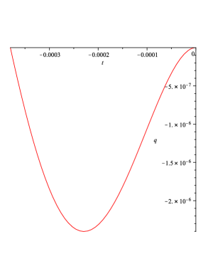
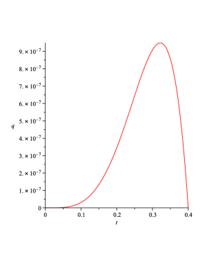
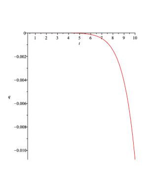
Figure 1: (1a Left) The deceleration parameter for inflation era of expansion history as a function of the t where t is the age of universe. (1b Middle) The deceleration parameter for deceleration era of expansion history as a function of the t where t is the age of universe. (1c Right) The deceleration parameter for late time acceleration era of expansion history as a function of the t where t is the age of universe.

In Figures 1a,1b and 1c, we sketch the deceleration parameter for three phases of expansion history as a function of the age of universe $t$. In these plots, we choose $t_{-}=-0.005(yr)$, $t_{+}=0.4(Gyr)$ and $t_{rip}=30(Gyr)$. We find that $q=-0.542$ leads to $t_{universe}=13.5(Gyr)$. This result is compatible with SNeIa data q22 . As it can be seen from Fig. 1a, the deceleration parameter is negative in the range $t_{-}<t<0$ and becomes zero at $t=0$. This means that the Universe inflates in this period of time. In Fig. 1b, we observe that $q$ is zero at t=0 and $t=t_{+}$ and has a maximum in this epoch. Finally, this parameter (Fig. 1c) is negative again in today acceleration epoch and tends to $-\infty$ at Big Rip singularity.

VI Summary and Discussion

In this paper, we proposed a model that allows to account for dynamics of the transition from the phantom inflationary to the non-phantom standard cosmology and to recover the today observed acceleration epoch. At the first stage of evolution, a BIon system is formed due to the dynamics of black fundamental strings at transition point. This BIon is a configuration in flat space of a universe brane and a parallel anti-brane connected by a wormhole. With decreasing temperature, wormhole becomes thinner, its energy flows into the universe branes and causes their growth. After a short time, this wormhole evaporates, inflation ends and non-phantom era begins. Eventually, two universe brane and antibrane become close to each other, tachyonic potential between them increases and a new wormhole is formed. In this condition, the Universe evolves from non-phantom phase to phantom one and consequently, a phantom-dominated era of the Universe accelerates and ends up into Big-Rip singularity. Comparing this model with previous unified cosmology models and observational data, it is possible to obtain some phenomenological parameters in terms of time. In a forthcoming paper, we will develop the model in view of cosmological observations adopting the approach discussed in q9 .