Variety of regimes of star-like networks of Hénon maps

Abstract

In this paper we categorize dynamical regimes demonstrated by star-like networks with chaotic nodes. This analysis is done in view of further studying of chaotic scale-free networks, since a star-like structure is the main motif of them. We analyze star-like networks of Hénon maps. They are found to demonstrate a huge diversity of regimes. Varying the coupling strength we reveal chaos, quasiperiodicity, and periodicity. The nodes can be both fully- and phase-synchronized. The hub node can be either synchronized with the subordinate nodes or oscillate separately from fully synchronized subordinates. There is a range of wild multistability where the zoo of regimes is the most various. One can hardly predict here even a qualitative nature of the expected solution, since each perturbation of the coupling strength or initial conditions results in a new character of dynamics.

I Introduction

Complex dynamical networks with scale-free coupling structure attract a lot of interest as models for a large variety of natural systems Boccaletti et al. (2006); Wang (2002). The name “scale-free” for these networks appears because their node degree distributions have power law shapes. As a result a small number of nodes hold a major balk of links while the rest of nodes have few connections Barabási et al. (2000).

One of the main questions arising in studying of these networks is the type and conditions of synchronization Boccaletti et al. (2006); Arenas et al. (2008); Osipov et al. (2007); Golubitsky and Stewart (2015). The synchronization can be full or only the phases of node oscillators can be synchronized; it can involve the whole bunch of nodes or the nodes can form synchronized clusters Wang (2002); Belykh et al. (2005); Arenas et al. (2006). Papers Wang and Chen (2002a); Fan and Wang (2005); Osipov et al. (2007); Arenas et al. (2008) are devoted to an analysis of synchronization conditions, works Jalan and Amritkar (2003); Jalan et al. (2005) investigate the formation of synchronization clusters while in Ref. Jalan et al. (2015) the impact of presence of a leader on the cluster synchronization is recovered. Paper Gambuzza et al. (2013) investigates so called remote synchronization when nodes can get synchronized even being connected indirectly though intermediate ones. Also this regime is studied in Refs. Jalan and Amritkar (2003); Jalan et al. (2005) being called driven synchronization.

Authors of Ref. Wang and Zhang (2010) study scale-free networks with fractional order oscillators. Paper Wang and Chen (2002b) investigates the control of a scale-free dynamical network by applying local feedback injections to a fraction of network nodes. Covariant Lyapunov vectors Kuptsov and Parlitz (2012) and their nonwandering predictable localization is studied in Ref. Kuptsov and Kuptsova (2014).

The feature specific for scale-free networks as well as for other complex dynamical networks is multistability Roxin et al. (2005); Angeli et al. (2004); Angeli (2009). It is well known that the dynamics of multistable systems can be amazingly rich Feudel (2008); Pisarchik and Feudel (2014). It occurs when the number of attractors is very high, and their basins have fractal boundaries that are highly interwoven. In this case the dynamics is very sensible to the initial state: even tiny perturbation results in arriving at new regime. Moreover, the ranges of existence of particular attractors can be narrow so that the qualitative behavior of the system can change dramatically when its parameters are slightly varied Feudel (2008). For scale-free networks this type of behavior was reported in Ref. Kuptsov and Kuptsova (2014). We suggest to refer to this type of dynamics as wild multistability to distinguish it form the plain case, when one can easily locate basins of the required attractors and put the system there to observe the expected behavior.

Wild multistability as well as other dynamical phenomena demonstrated by dynamical networks still requires an exhaustive study. In particular the interesting question is to reveal what features are the same with other systems and what additionally emerge due to the strong inhomogeneity of networks. For scale-free networks the this study can be started from the consideration of their simplest and regular representatives which are star-like structures. These structures consist of the hub node connected with all other nodes and subordinate nodes that have only one connection with the hub. Star-like structures are the main motifs of scale-free networks, their building blocks.

Chaotic synchronization of oscillator networks with star-like couplings is considered in Ref. Pecora (1998). Formation of synchronized clusters in such networks is studied in Ref. Ma et al. (2008) and a sufficient condition about the existence and asymptotic stability of a cluster synchronization invariant manifold is derived. Paper Bergner et al. (2012) considers phase synchronization of the subordinates when the hub is not synchronized with them. This is called remote synchronization.

Thus, to pave the way to understanding the dynamics of scale-free networks, one has to reveal first the details of dynamics of systems with star-like coupling. This is the main motivation for the present paper. We consider Hénon maps. This map is a canonical model that is sufficiently simple on the one hand and exhibit the same essential properties as much more “serious” chaotic system on the other hand Hénon (1976). In particular, this map is time-reversible, and the coupling between network nodes is introduced in a way preserving this property. Altogether, we build a catalog of regimes of time-reversible star-like network of Hénon maps observed at different coupling strengths. The most of the regimes are found to be independent on the network size. However there is an area of wild multistability where the dynamics does depend on the number of nodes. Many different attractors exist here within a narrow ranges. As a result, one can hardly predict even a qualitative nature of the expected solution, since each perturbation of coupling strength or initial conditions leads to a new character of dynamics.

The outline of the paper is the following. First we introduce the model system. Then we discuss the numerical criteria for detecting various synchronization regimes. After that the registered regimes are represented and discussed. Finally, the ranges of stability of some of the regimes are derived.

II Model system

We consider a network of Hénon maps introduced in Ref. Kuptsov and Kuptsova (2014) as a generalization of the Hénon chain from Ref. Politi and Torcini (1992):

$$\begin{gathered}x_{n}(t+1)=\alpha-[x_{n}(t)+\epsilon h_{n}(t)]^{2}+y_{n}(t),\\ y_{n}(t+1)=\beta x_{n}(t),\\ h_{n}(t)=\sum_{j=1}^{N}\frac{a_{nj}}{k_{n}}x_{j}(t)-x_{n}(t),\;k_{n}=\sum_{j=1}^{N}a_{jn}.\end{gathered}$$ (1)

Here $N$ is the number of network nodes, $t=0,1,2\ldots$ is discrete time, $a_{nj}\in\{0,1\}$, $a_{nj}=a_{jn}$, $a_{nn}=0$ are the elements of the $N\times N$ adjacency matrix $\mathrm{A}$, and $k_{n}$ is degree of the $n$th node, i.e., the number of its connections. $\alpha=1.4$ and $\beta=0.3$ are the parameters controlling local dynamics, and $\epsilon\in[0,1]$ is the coupling strength. Recall that the Hénon map is time-reversible. The coupling is introduced in a way that preserves this property.

We consider star-like networks, see Fig. 1. Let $\mbox{\boldmath{$\mathrm{e}$}}_{m,m}$ be a unit $m\times m$ matrix, $\mbox{\boldmath{$\mathrm{z}$}}_{m,n}$ be a $m\times n$ matrix of zeros, and $\mbox{\boldmath{$\mathrm{d}$}}_{m,n}$ be a $m\times n$ matrix of ones. Using this notation the adjacency matrix can written in block form as

$$\mbox{\boldmath{$\mathrm{A}$}}=\begin{pmatrix}\mbox{\boldmath{$\mathrm{z}$}}_{1,1}&\mbox{\boldmath{$\mathrm{d}$}}_{1,M}\\ \mbox{\boldmath{$\mathrm{d}$}}_{M,1}&\mbox{\boldmath{$\mathrm{z}$}}_{M,M}\end{pmatrix}$$ (2)

where $M=N-1$.

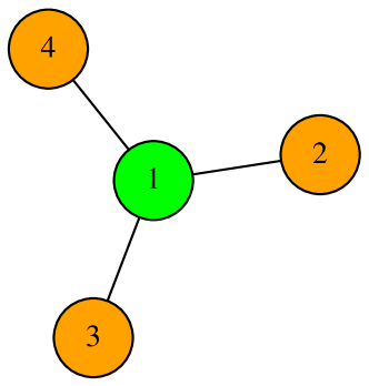
Figure 1: (color online) The star-like network, $N=4$.

In numerical simulations some regimes was found to emerge outside the theoretical ranges of stability, computed in Sec. V. In particular this is the case for full chaotic synchronization. This spurious stability occurs due to round-off errors in numerical model. To eliminate it a very weak noise is added to system variables:

$$x_{n}(t)\to x_{n}(t)+\xi(2t),\;y_{n}(t)\to y_{n}(t)+\beta\xi(2t+1),$$ (3)

where $\xi(t)\in(-10^{-12},10^{-12})$. Notice that the noise is added only to fix the drawback of the numerical model. Since its amplitude is not much higher then the machine epsilon for employed variables, $\approx 10^{-16}$, it is indistinguishable in the resulting time series. Thus, we emphasize that the study of noise influence on the network lies outside the scope of our paper.

III Criteria of synchronization

Coincidence of local extrema of two discrete time signals can be treated as their phase synchronization while the relative frequency of the coincidences quantifies the degree of the synchronization Jalan and Amritkar (2003); Jalan et al. (2005). Below we consider a generalization of this approach taking into account both dip-dip and peak-dip coincidences.

Let us consider the nodes $m$ and $n$, $m<n$. Given a starting time $t_{0}$ and the interval $\mathcal{T}$, count at $t_{0}\leq t<t_{0}+\mathcal{T}$ the numbers $\nu_{m}$ and $\nu_{n}$ of local minima of $x_{m}(t)$ and $x_{n}(t)$, respectively, and the number $\nu_{mn}$ of simultaneous minima of $x_{m}$ and $x_{n}$. In addition we count the number of times $\mu_{mn}$ when the local minima of $x_{m}$ occur simultaneously with the local maxima of $x_{n}$, and the number of times $\mu_{nm}$ when the minima of $x_{n}$ coincide with the maxima of $x_{m}$. Note that since $m<n$, $\mu_{mn}$ can be treated as elements of the upper triangle of a square matrix and $\mu_{nm}$ form its lower triangle. Then the dip-dip distance can be computed as

$$d^{\,\text{d}}_{m\text{-}n}=\begin{cases}1-\nu_{mn}/\max\{\nu_{m},\nu_{n}\}&\text{if }\max\{\nu_{m},\nu_{n}\}>0,\\ 0&\text{if }\max\{\nu_{m},\nu_{n}\}=0.\end{cases}$$ (4)

The second choice covers the situation when both $x_{m}$ and $x_{n}$ do not oscillate at all. This value is introduced in Refs. Jalan and Amritkar (2003); Jalan et al. (2005) as phase distance. Analogously we can define peak-dip distance as

$$d^{\,\text{p}}_{m\text{-}n}=\begin{cases}1-\mu_{mn}/\max\{\nu_{m},\nu_{n}\}&\text{if }\max\{\nu_{m},\nu_{n}\}>0,\\ 0&\text{if }\max\{\nu_{m},\nu_{n}\}=0.\end{cases}$$ (5)

Two nodes are did-dip or peak-dip synchronized on the interval $\mathcal{T}$ if $d^{\,\text{d}}_{m\text{-}n}=0$ or $d^{\,\text{p}}_{m\text{-}n}=0$, respectively.

The full synchronization can be detected using $d^{\,\text{f}}_{m\text{-}n}$:

$$d^{\,\text{f}}_{m\text{-}n}=\mathop{\mathrm{Var}}\{x_{m}(t)-x_{n}(t)\;|\;t_{0}\leq t<t_{0}+\mathcal{T}\},$$ (6)

where $\mathop{\mathrm{Var}}$ stands for variance. Moreover we are going to detect complementary synchronization via the vanish of $d^{\,\text{c}}_{m\text{-}n}$:

$$d^{\,\text{c}}_{m\text{-}n}=\mathop{\mathrm{Var}}\{x_{m}(t)+x_{n}(t)\;|\;t_{0}\leq t<t_{0}+\mathcal{T}\}.$$ (7)

The synchronization is actually registered when $d^{\,\text{f}}_{m\text{-}n}$ or $d^{\,\text{c}}_{m\text{-}n}$ are below the threshold $10^{-12}$, which the level of the added noise, see Eq. (3).

All of the above criteria depend on $\mathcal{T}$. It determines the resolution of the detection procedure. If $\mathcal{T}\to\infty$ the procedure responds only to full-time regimes. So it is preferable for $\mathcal{T}$ to be as short as possible. In this case in addition to full-time synchronization, one can detect synchronization windows as series of subsequent intervals where $d^{\,\text{d}}_{m\text{-}n}$, $d^{\,\text{p}}_{m\text{-}n}$, $d^{\,\text{f}}_{m\text{-}n}$, or $d^{\,\text{c}}_{m\text{-}n}$ vanish. The lower boundary for $\mathcal{T}$ is the average interval between peaks and dips: $\mathcal{T}$ has to be large enough to catch at least two-three of them. In simulations below we set $\mathcal{T}=16$.

IV Classification of dynamical regimes

IV.1 Method of analysis

Since it is unclear a priori what types of behaviour can be observed, the most reliable way is the visual inspection of time series corroborated by some appropriate characteristic numbers.

First of all we are going to employ the first Lyapunov exponent whose positive value indicates chaos, the negative sign reveals periodicity and the zero means quasi-periodicity. One has to take many random initial conditions and compute $\lambda_{1}$ for each corresponding trajectory. The resulting values are grouped very well near a few points representing different regimes. This approach is usually used for analysis of multistability Pisarchik and Feudel (2014).

Various types of synchronous oscillations will be detected using criteria introduced in Sec. III. We take $\mathcal{T}=16$ and test at each subsequent interval $\mathcal{T}$ if one of the four characteristic values vanishes for each pair of oscillators. If yes, we are inside a window of synchronization of a corresponding type. Then we find the largest lengths of the windows that are registered along the observation time, which is $t_{\text{max}}=10^{5}\mathcal{T}$. The full-time synchronization is registered if the corresponding window lasts during the whole observation time $t_{\text{max}}$.

IV.2 The star with $N=4$

Consider dynamics of the network (1), (2) when the coupling $\epsilon$ varies from 0 to 1. We have inspected all values of $\epsilon\in[0,1]$ with the step $0.01$ for the smallest nontrivial star $N=4$. Moreover when a regime of some sort appeared only on a single step, we also checked if it existed at least in a small vicinity of the corresponding $\epsilon$ to make sure that this is a typical situation. To detect a multistability, for each $\epsilon$ we tested at least 200 random initial conditions. The results are gathered in Figs. 2 and 3 that are discussed below.

To facilitate the referencing we will label the regimes with three letters. The first two ones are an abbreviation describing a type of synchronization between network nodes. In some cases we will supply them with a subscript to show a number of involved nodes. The third letter indicates the character of oscillations: periodic “P”, quasiperiodic “Q”, chaotic “C”. If there are several regimes with identical abbreviations we also add an index number. The exception to this scheme is the oscillation death that will be labeled merely as OSD.

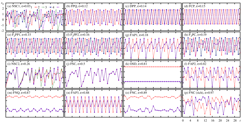
Figure 2: (color online) Various regimes of the star-like network (1), (2) with $N=4$. See details in the text.

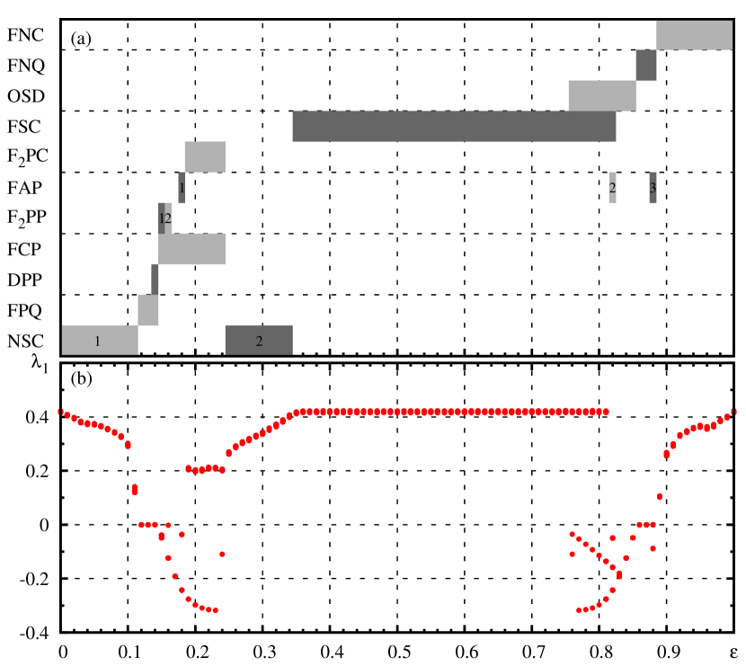
Figure 3: (color online) (a) An ordering of the regimes shown in Fig. 2. See also Tab. 1. (b) The first Lyapunov exponents computed for 200 random initial conditions at each $\epsilon=0,0.01,0.02,\ldots,1$

Table 1: Stability ranges of $\epsilon$ for regimes in Figs. 2 and 3 obtained via step by step analysis of dynamics with $\Delta\epsilon=0.01$. More accurate values for FSC, OSD and FCP are found in Sec. V, see Eqs. (14), (21), and (26), respectively.

NSC:	[0,0.11], [0.25,0.34]	FPQ:	[0.12,0.14]
DPP:	0.14	FCP:	[0.15,0.24]
F2PP:	0.15, 0.16	FAP:	0.18, 0.82, 0.88
F2PC:	[0.19,0.24]	FSC:	[0.35,0.82]
OSD:	[0.76,0.85]	FNQ:	[0.86,0.88]
FNC:	[0.89,1]

The ordering of the regimes is shown in Fig. 3(a), and the boundaries of the regimes are collected in Tab. 1. Fig. 3(b) shows $\lambda_{1}$ vs. $\epsilon$ computed for 200 random initial conditions.

• $\epsilon=0,0.01,\ldots,0.11$:  NSC1. There is only one chaotic attractor here. This is confirmed by the coincidence in Fig. 3(b) of Lyapunov exponents, and by visual inspection of time series whose typical example is shown in Fig. 2(a). The power law divergence of peak-dip synchronization windows between the hub and subordinates and dip-dip windows for the subordinates, see Figs. 4(a) and (b), indicate the intermittency appearing near the right boundary of the considered range.

• $\epsilon=0.12,0.13$:  FPQ, Fig. 2(b). The quasiperiodicity is confirmed by the vanish of $\lambda_{1}$ in Fig. 3(b).

• $\epsilon=0.14$:  FPQ and DPP, Fig. 2(c). Actually in DPP two subordinates are fully synchronized while the third one, the node number 4, almost coincides with them. The Lyapunov exponent corresponding to DPP is close to zero, $\lambda_{1}=-0.00030$, and one can not distinguish it in Fig. 3(b). However, the inspection of data reveals that it is strictly smaller then the Lyapunov exponent for FPQ, so that despite of FPQ this regime is periodic. Moreover, we computed Fourier spectra (not shown), that again confirmed the quasiperiodicity of FPQ and the periodicity of DPP.

• $\epsilon=0.15$:  FCP and F₂PP1. See Figs. 2(d) and (e), respectively. The dominating regime here is FCP. It exists within a wide range of $\epsilon$, see Tab 1. In Fig. 3(b) it corresponds to the lowest branch of the Lyapunov exponents. The F₂PP1 has smaller basing of attraction and exists within a narrow range of $\epsilon$ around $0.15$. At $\epsilon=0.15$ the Lyapunov exponents for these two regimes though different, are close to each other and barely distinguishable in Fig. 3(b): for FCP $\lambda_{1}=-0.0487$ and for F₂PP1 $\lambda_{1}=-0.0389$.

• $\epsilon=0.16$:  FCP and F₂PP2. Here we have the second version of the periodic regime with full synchronization of two subordinates, see Fig. 2(f). Though it looks like F₂PP1, the closer inspection reveals that the period of F₂PP1 is 6 and the period of F₂PP2 is 20. The first Lyapunov exponent for F₂PP2 is $\lambda_{1}=-0.00191$.

• $\epsilon=0.17$:  FCP.

• $\epsilon=0.18$:  FCP and FAP1, Fig. 2(g). The Lyapunov exponents are $\lambda_{1}=-0.243$, and $\lambda_{1}=-0.0360$, respectively.

• $\epsilon=0.19,\ldots,0.24$:  FCP and F₂PC, Fig. 2(h). The emergence of the second regime is clearly seen in Fig. 3(b), where the upper branch of positive Lyapunov exponents appears near $0.2$. Note that $\lambda_{1}$ for F₂PC is rather independent on $\epsilon$.

• $\epsilon=0.25,\ldots,0.34$:  NSC2, Fig. 2(i). In the second version of these regime we again observe an intermittency. When $\epsilon$ approaches the right boundary of the range the full synchronization windows demonstrate power law divergence, see Fig. 4(c,d).

• $\epsilon=0.35,\ldots,0.75$:  FSC, Fig. 2(j). In Fig. 3(b) this regime is represented by a perfect horizontal line.

• $\epsilon=0.76,\ldots,0.81$:  FSC and OSD, Fig. 2(k). OSD has very small basin of attraction here. It becomes more or less easily detectable only at $\epsilon=0.81$. There are two forms of OSD. The second one, not shown, is an interchange of the values for the hub and subordinate node variables. Two forms have different negative Lyapunov exponents, so that there are three branches in Fig. 3(b), one positive for FSC and two negative for OSD.

• $\epsilon=0.82$:  FSC, OSD, and FAP2, Fig. 2(l). Accordingly, there are four values of Lyapunov exponents, see Fig. 3(b): $\lambda_{1}=-0.243$ and $-0.158$ for OSD, $\lambda_{1}=-0.0492$ for FAP2, and $\lambda_{1}=0.419$ for FSC.

• $\epsilon=0.83$:  OSD. The Lyapunov exponents corresponding to the two forms of OSD becomes very close to each other, $\lambda_{1}=-0.192$ and $\lambda_{1}=-0.182$. Right after this point they merge, see Fig. 3(b).

• $\epsilon=0.84,0.85$:  OSD. Now both forms of this regime have identical Lyapunov exponents, see Fig. 3(b).

• $\epsilon=0.86,87$:  FNQ. This regime appears when two fixed points corresponding to OSD become unstable, see Fig. 2(m). The corresponding Lyapunov exponent is zero here, see Fig. 3(b).

• $\epsilon=0.88$:  FNQ, FAP3, Fig. 2(n). The Lyapunov exponents are zero for FNQ and $\lambda_{1}=-0.0888$ for FAP3, see Fig. 3(b).

• $\epsilon=0.89,\ldots,1$:  FNC. Starting from this point the oscillations born from OSD fixed points become chaotic. Initially the oscillations have sufficiently small amplitude, see Fig. 2(o), and as $\epsilon$ grows the oscillations become more and more entangled, see Fig. 2(p).

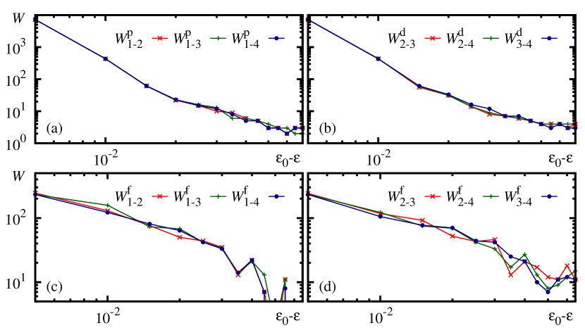
Figure 4: (color online) Longest synchronization windows vs. coupling near the boundaries of ranges. (a,b) NSC1, $\epsilon_{0}=0.115$; (c,d) NSC2, $\epsilon_{0}=0.345$. $W^{\,\text{d}}_{m\text{-}n}$, $W^{\,\text{p}}_{m\text{-}n}$, and $W^{\,\text{f}}_{m\text{-}n}$ denote the lengths of the longest windows where corresponding $d^{\,\text{d}}_{m\text{-}n}$, $d^{\,\text{p}}_{m\text{-}n}$, and $d^{\,\text{f}}_{m\text{-}n}$ vanish.

IV.3 Stars with $N>4$ and wild multistability

Figure 5 compares first Lyapunov exponents computed for stars of different sizes. Observe remarkable coincidence of almost all points, indicating the identity of dynamics regardless of $N$. Additionally we verified it by visual inspection of time series and by the analysis of synchronization windows. Moreover, below we will provide rigorous proofs for certain regimes that their ranges of stability do not depend on $N$.

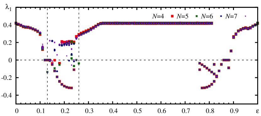
Figure 5: (color online) The fist Lyapunov exponents for $N=4,5,6$ and $7$. Data for $N=4$ are the same as in Fig. 3(b). Vertical lines at $\epsilon=0.13$ and $0.26$ mark an area of wild multistability where the Lyapunov exponents for different $N$ do not coincide.

However, one have also to notice the area where $\lambda_{1}$ does depend on $N$. This area is marked in Fig. 5 by dashed vertical lines. Some of attractors like FPQ ($\lambda_{1}=0$) and FCP (the lowest branch of $\lambda_{1}$) still exists regardless of $N$. But in addition a variety of other attractors appears only at certain $N$, each with a narrow range of stability on $\epsilon$.

Figure 6 illustrates what can be encountered within this area. Figure 6(a) demonstrates a periodic regime with $\lambda_{1}=-0.136$, emerging at $N=5$, and $\epsilon=0.13$. Here the subordinates are fully synchronized by pairs: $d^{\,\text{f}}_{2\text{-}5}=0$, and $d^{\,\text{f}}_{3\text{-}4}=0$. These pairs in turn are dip-dip synchronized with each other, $d^{\,\text{d}}_{2,3\text{-}4,5}=0$. The hub is in peak-dip synchronization with all subordinates, $d^{\,\text{p}}_{1\text{-}2,3,4,5}=0$. Figure 6(b) represents a chaotic regime at $N=7$ and $\epsilon=0.24$ with $\lambda_{1}=0.00206$. Four of six subordinates, namely 4,5,6, and 7, are fully synchronized. Two others, 2 and 3, are dip-dip synchronized with each other. This pair is in turn in peak-dip synchronization with the other four. The hub is dip-dip synchronized with the nodes 2 and 3 and peak-dip synchronized with the other four.

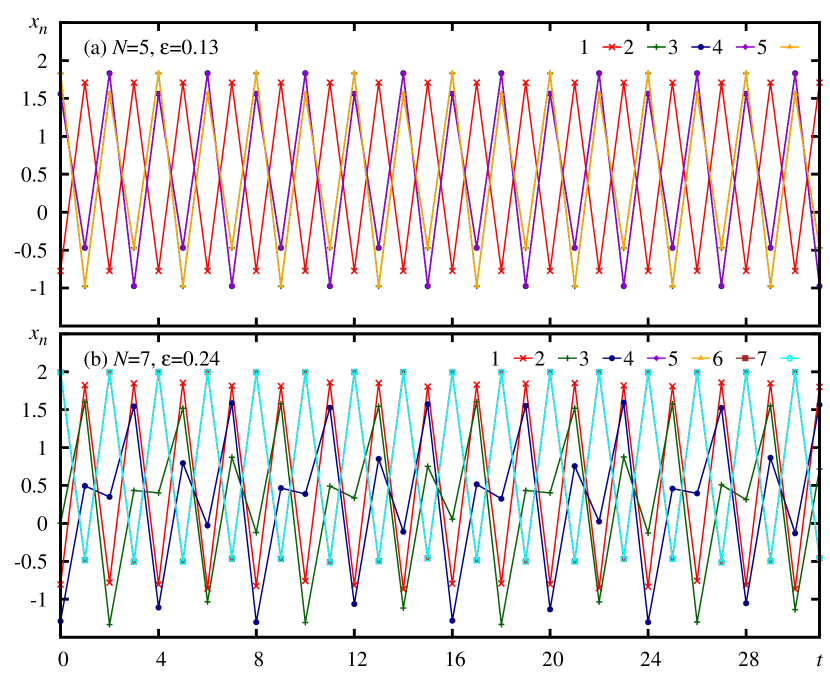
Figure 6: (color online) Examples of dynamics of the star-like networks with $N>4$ within the range of wild multistability. (a) $N=5$, $\epsilon=0.13$ (b) $N=7$, $\epsilon=0.24$

Altogether, within the area delimited by the dashed lines in Fig. 5 there is the large number of attractors with highly interwoven basins and narrow stability ranges. As a result one can hardly predict the qualitative nature of the expected dynamics since each perturbation to $\epsilon$ or initial condition results in quite different behavior. Similar situation was already reported for systems with high dimensional phase space, in particular, for coupled map lattices, see the review in Ref. Feudel (2008). We suggest to refer to it as wild multistability to emphasize its amazing richness.

One more similar area is located in Fig. 5 between $\epsilon\approx 0.8$ and $\epsilon\approx 0.9$. Though the Lyapunov exponents do not depend on $N$ here, the basins of coexisting attractors can be colocated in complicated manner impeding prediction of the dynamics.

IV.4 Remote synchronization

As we already mentioned above, remote synchronization occurs between two or more nodes without direct connections, but linked with the common hub node. The important point here is that the hub remains not synchronized with them, that is achieved by detuning its natural frequency Bergner et al. (2012); Gambuzza et al. (2013).

In our case there are regimes with fully synchronous subordinates and the hub not coinciding with them. These are FPQ, DPP, FCP, all F₂PPs, all FAPs, and F₂PC, see Fig. 2. This behavior though reminds remote synchronization, can not be classified like this since actually the hub is also synchronized with the rest of nodes with a phase shift.

The remote synchronization is nevertheless observed for our system, see FNQ and FNC in Figs. 2(m) and (o,p), respectively. These regimes essentially differ from those reported in Ref. Bergner et al. (2012). First, the subordinates are fully synchronized, while in Ref. Bergner et al. (2012) phase synchronization is reported. Second, in our case oscillators are identical, but the hub still does not get synchronized with the subordinates. Third, FNQ and FNC are quasiperiodic and chaotic regimes, respectively, contrary to the periodic case reported in Bergner et al. (2012). For these regimes the difference between the hub and subordinates is found to be not necessary to prevent their synchronization.

V Stability of certain regimes

V.1 Full chaotic synchronization (FSC)

Stability of the fully synchronized state can be analyzed using so called Master Stability Function (MSF) Pecora and Carroll (1998); Boccaletti et al. (2006); Pecora (1998). First we need the Jacobian matrix of the network (1). It has a block form being composed of $N\times N$ matrices:

$$\mbox{\boldmath{$\mathrm{J}$}}(t)=\begin{pmatrix}\mbox{\boldmath{$\mathrm{F}$}}(t)&\mbox{\boldmath{$\mathrm{I}$}}\\ \beta\mbox{\boldmath{$\mathrm{I}$}}&0\end{pmatrix},$$ (8)

where

$$\begin{gathered}\mbox{\boldmath{$\mathrm{F}$}}(t)=-2\mbox{\boldmath{$\mathrm{G}$}}(t)\,[(1-\epsilon)\mbox{\boldmath{$\mathrm{I}$}}+\epsilon\mbox{\boldmath{$\mathrm{K}$}}^{-1}\mbox{\boldmath{$\mathrm{A}$}}],\\ \mbox{\boldmath{$\mathrm{G}$}}(t)=\mathop{\mathrm{diag}}\{x_{n}+\epsilon h_{n}\},\;\mbox{\boldmath{$\mathrm{K}$}}=\mathop{\mathrm{diag}}\{k_{n}\},\end{gathered}$$ (9)

and $\mathrm{I}$ is the identity matrix Kuptsov and Kuptsova (2014).

Jacobian matrix at $x_{n}(t)\to x(t)$ governs the evolution of tangent perturbation to the synchronization manifold, where $x(t)$ is produced by a local isolated oscillator. Decomposing the perturbations over eigenvectors of the matrix $(\mbox{\boldmath{$\mathrm{K}$}}^{-1}\mbox{\boldmath{$\mathrm{A}$}})$ one obtains the following equations for perturbation amplitudes:

$$\delta p(t+1) =-\nu[2x(t)\delta p(t)]+\delta q(t),$$ (10)

$$\delta q(t+1) =\beta\,\delta p,$$

where

$$\nu=1+\epsilon\,(\phi-1),$$ (11)

and $\phi$ is an eigenvalue of $(\mbox{\boldmath{$\mathrm{K}$}}^{-1}\mbox{\boldmath{$\mathrm{A}$}})$. We can treat $\nu$ a free parameter and define MSF as a conditional Lyapunov exponent, i.e., an average rate of exponential growth of a solution of Eq. (10) when $x(t)$ runs along a trajectory of the local oscillator. The graph of MSF is shown in Fig. 7. Note that MSF is negative at $|\nu|<0.652$.

Figure 7: (color online) MSF for the network (1), (2). Vertical dotted lines delimit an area where MSF is negative.

Using Eq. (2), one can rewrite matrix $(\mbox{\boldmath{$\mathrm{K}$}}^{-1}\mbox{\boldmath{$\mathrm{A}$}})$ as

$$\mbox{\boldmath{$\mathrm{K}$}}^{-1}\mbox{\boldmath{$\mathrm{A}$}}=\begin{pmatrix}\mbox{\boldmath{$\mathrm{z}$}}_{1,1}&\mbox{\boldmath{$\mathrm{d}$}}_{1,M}/M\\ \mbox{\boldmath{$\mathrm{d}$}}_{M,1}&\mbox{\boldmath{$\mathrm{z}$}}_{M,M}\end{pmatrix},$$ (12)

and then compute its eigenvalues:

$$\phi_{1}=1,\phi_{2}=-1,\phi_{3}=\phi_{4}=\cdots=\phi_{N}=0$$ (13)

The eigenvector corresponding to $\phi_{1}$ has identical elements being responsible for chaotic dynamics on the synchronization manifold. All other eigenvectors and eigenvalues correspond to transverse perturbations whose vanish is the necessary condition of stability of the full synchronization.

Substituting $\phi=-1$ and $\phi=0$ to Eq. (11), one can see that MSF is negative for all transverse perturbations when

$$\epsilon=\epsilon_{\text{FSC}}\in[0.348,0.826].$$ (14)

Withing this range the full synchronization attractor is transversely stable on average. For attractors with regular structure this is also a sufficient condition, but when the dynamics is chaotic, the synchronization can be destabilized by a small noise even when MSF is negative. This is due to the presence of transversally unstable invariant sets (cycles, in particular) embedded into the synchronization manifold, see Milnor (2004). In our case however the influence of noise (3) is indistinguishably weak. One can see in Fig. 3(b) that the first Lyapunov exponent attains the level corresponding to this regime almost exactly within the range (14).

Note that the stability range for the full chaotic synchronization does not depend on $N$. The reason is that the matrix $(\mbox{\boldmath{$\mathrm{K}$}}^{-1}\mbox{\boldmath{$\mathrm{A}$}})$ has only three different eigenvalues $1$,$-1$, and $0$ regardless of $N$.

V.2 Oscillations death (OSD)

Let $x_{a}$ and $x_{b}$ be states of the hub and the subordinates at OSD, respectively. Using Eqs. (1), one can write:

$$x_{a} =\alpha-[x_{a}+\epsilon(x_{b}-x_{a})]^{2}+\beta x_{a},$$ (15)

$$x_{b} =\alpha-[x_{b}+\epsilon(x_{a}-x_{b})]^{2}+\beta x_{b}.$$

The solution of these equations can be expressed via roots $\xi_{1}$ and $\xi_{2}$ of the polynomial

$$\xi^{2}+\frac{\beta-1}{2\epsilon-1}\xi+\frac{((\beta-1)^{2}-4\alpha)\epsilon^{2}+\alpha(4\epsilon-1)}{(2\epsilon-1)^{4}}=0.$$ (16)

There are two couples, $x_{a}=\xi_{1}$, $x_{b}=\xi_{2}$, and $x_{a}=\xi_{2}$, $x_{b}=\xi_{1}$, corresponding to two forms of OSD.

Stability of the OSD solution is determined by eigenvalues $\mu$ of the Jacobian matrix (8) at ($x_{a}$, $x_{b}$). The eigenvalue problem for $\mu$ is reduced to

$$\mu^{2}-\mu f-\beta=0,$$ (17)

where $f$ is an eigenvalue of $\mathrm{F}$, see Eq. (9). One can see that each $f$ produces a couple of $\mu$. Computing $f$ we employ the block representation of $\mathrm{A}$ (2):

$$\mbox{\boldmath{$\mathrm{F}$}}=\begin{pmatrix}\kappa_{a}(1-\epsilon)\mbox{\boldmath{$\mathrm{e}$}}_{1,1}&(\kappa_{a}\epsilon/M)\mbox{\boldmath{$\mathrm{d}$}}_{1,M}\\ \kappa_{b}\epsilon\mbox{\boldmath{$\mathrm{d}$}}_{M,1}&\kappa_{b}(1-\epsilon)\mbox{\boldmath{$\mathrm{e}$}}_{M,M}\end{pmatrix}.$$ (18)

Here $\kappa_{a}=x_{a}+\epsilon(x_{b}-x_{a})$ corresponds to the hub node and $\kappa_{b}=x_{b}+\epsilon(x_{a}-x_{b})$ comes from the subordinates. The eigenproblem for $\mathrm{F}$ results in

$$[f+2\kappa_{a}(1-\epsilon)][f+2\kappa_{b}(1-\epsilon)]M=4\kappa_{a}\kappa_{b}\epsilon^{2}\delta.$$ (19)

Here $\delta$ is one of eigenvalues of $\mbox{\boldmath{$\mathrm{d}$}}_{M,M}$,

$$\delta_{1}=M,\delta_{2}=\delta_{3}=\cdots=\delta_{M}=0.$$ (20)

Each $\delta=0$ produces a couple of solutions of Eq. (19). However, $f=-2\kappa_{a}(1-\epsilon)$ is spurious that can be verified by substituting it to the eigenproblem for $\mathrm{F}$. Thus $\mathrm{F}$ has the eigenvalue $f=-2\kappa_{b}(1-\epsilon)$ with the multiplicity $M-1$. Two more eigenvalues correspond to $\delta=M$. They can be found from Eq. (19) by canceling $M$. Note that none of $f$ depends on the number of the network nodes.

To obtain the stability range for OSD one has to vary $\epsilon$, compute $f$, and find the absolute values of corresponding eigenvalues $\mu$ from Eq. (17). The regime is stable when $|\mu|<1$. Figure 8 shows the plots of the largest by magnitude $|\mu|$. In the middle area the curves vanish because Eq. (16) has complex roots. Thus the range of stability computed in this way is

$$\epsilon=\epsilon_{\text{OSD}}\in[0.757,0.856].$$ (21)

It agrees well with the range obtained via straightforward simulations, see Tab. 1.

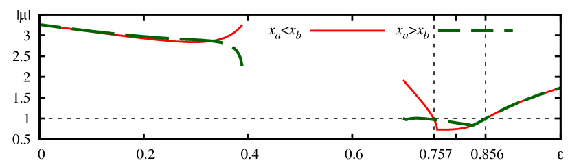
Figure 8: (color online) The largest by magnitude eigenvalue of the Jacobian matrix (8), (9) for OSD. Vertical lines delimit the range of stability.

V.3 Full synchronization of the subordinates, and complementary synchronization of the hub with them (FCP)

In this regime the system oscillates with period two so that the hub and the coinciding subordinates switch between $x_{a}$ and $x_{b}$:

$$x_{a} =\alpha-[x_{b}+\epsilon(x_{a}-x_{b})]^{2}+\beta x_{a},$$ (22)

$$x_{b} =\alpha-[x_{a}+\epsilon(x_{b}-x_{a})]^{2}+\beta x_{b}.$$

Solutions to this equation set can be found as roots of the polynomial

$$\xi^{2}-\frac{\beta-1}{2\epsilon-1}\xi+\frac{(1-\epsilon)[(1-\beta)^{2}(1-\epsilon)+4\alpha\epsilon]-\alpha}{(2\epsilon-1)^{4}}=0.$$ (23)

Stability of FCP is determined by the eigenvalues $\mu$ of the matrix $(\mbox{\boldmath{$\mathrm{J}$}}_{b}\mbox{\boldmath{$\mathrm{J}$}}_{a})$ where $\mbox{\boldmath{$\mathrm{J}$}}_{a}$ is computed as in Sec. V.2, and $\mbox{\boldmath{$\mathrm{J}$}}_{b}$ is similar on interchanging $x_{a}$ and $x_{b}$:

$$(\mu-\beta)^{2}=f\mu,$$ (24)

where $f$ is an eigenvalue of the matrix product $(\mbox{\boldmath{$\mathrm{F}$}}_{b}\mbox{\boldmath{$\mathrm{F}$}}_{a})$.

Using Eq. (18) one can write the matrix $(\mbox{\boldmath{$\mathrm{F}$}}_{b}\mbox{\boldmath{$\mathrm{F}$}}_{a})$ explicitly and find that its eigenproblem results in the equation

$$(f-a_{11})(f-b_{22})M=(a_{22}f-a_{11}a_{22}+a_{12}a_{21})\delta,$$ (25)

where $a_{11}=\kappa_{b}[\kappa_{a}(1-\epsilon)^{2}+\kappa_{b}\epsilon^{2}]$, $a_{12}=\kappa_{b}(\kappa_{a}+\kappa_{b})\epsilon(1-\epsilon)$, $a_{21}=\kappa_{a}(\kappa_{a}+\kappa_{b})\epsilon(1-\epsilon)$, $a_{22}=\kappa_{a}^{2}\epsilon^{2}$, $b_{22}=\kappa_{a}\kappa_{b}(1-\epsilon)^{2}$, and $\delta$ is an eigenvalue of $\mbox{\boldmath{$\mathrm{d}$}}_{M,M}$, see Eq. (20). The root $f=a_{11}$ at $\delta=0$ is spurious that can be tested by a direct substitution. Thus there is an eigenvalue $f=b_{22}$ with the multiplicity $M-1$ and two more eigenvalues are the solutions of Eq. (25) at $\delta=M$. Notice, that as in Sec. V.2, $M$ is canceled so that the stability range again does depend of the network size.

Varying $\epsilon$ we can compute $f$ and then find the largest $|\mu|$. The plot is shown in Fig. 9. The FCP regime is stable where $|\mu|<1$. This range is

$$\epsilon=\epsilon_{\text{FCP}}\in[0.143,0.244].$$ (26)

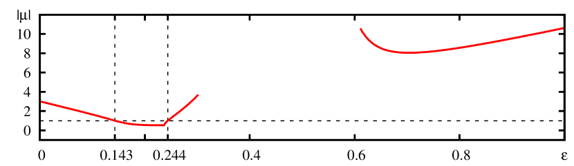
Figure 9: (color online) The largest by magnitude eigenvalue of the Jacobian matrix for the regime FCP. Vertical lines delimit the range of stability.

VI Outline and conclusions

We considered a variety of dynamics of Hénon map networks with star-like topology. This is found to be amazingly rich. In brief, as the coupling strength grows from zero to one the following areas are observed.

• Non-synchronized oscillations, intermittency of synchronization windows.

• Quasiperiodicity.

• Wild multistability. Small variations of initial conditions result in periodic, quasiperiodic and chaotic solutions. The zoo of regimes is very sensitive both to variations of the coupling strength and to the network size.

• Again non-synchronized oscillations, intermittency of synchronization windows.

• Full chaotic synchronization of all network nodes.

• Coexistence of the full chaotic synchronization, oscillation death and periodic oscillations when the hub oscillates in anti-phase with fully synchronized subordinates.

• Oscillation death.

• Remote synchronization of quasiperiodic oscillations. At narrow range of coupling values it coexists with another version of the regime of periodic oscillations when the hub is in anti-phase with fully synchronized subordinates.

• Remote synchronization of chaotic oscillations.

We conjecture that the list of regimes and corresponding stability ranges in most cases remain the same regardless of $N$. This is checked numerically for $N\leq 7$ and rigorously proved for certain regimes. The exception is the wild multistability area where the dynamics is very sensitive to variations of $N$.

The considered networks demonstrates new examples of remote synchronization. These are quasiperiodic and chaotic regimes. For these regimes the non-identity of the hub and the subordinate nodes is not required to prevent their synchronization.

The most interesting situation occurs in the wild multistability area. Similar type of dynamics was already reported for other systems, in particular for coupled map lattices. We suggest to refer to it as wild multistability because of its complexity and richness. In fact one can hardly predict here even a qualitative nature of the expected solution. Each deviation in initial conditions and coupling strength value is found to result in a new character of dynamics. This can be either periodic, quasiperiodic, or chaotic regimes. Obviously a lot of interesting problems arise in this connection. Since star-like motifs are the basic building blocks of scale-free networks, the detailed study of wild multistability area is very important for further understanding of the dynamics of complex scale-free networks.

References

- Boccaletti et al. (2006) S. Boccaletti, V. Latora, Y. Moreno, M. Chavez, and D.-U. Hwang, Physics Reports 424, 175 (2006).
- Wang (2002) X. F. Wang, International Journal of Bifurcation and Chaos 12, 885 (2002).
- Barabási et al. (2000) A.-L. Barabási, R. Albert, and H. Jeong, Physica A 281, 69 (2000).
- Arenas et al. (2008) A. Arenas, A. Díaz-Guilera, J. Kurths, Y. Moreno, and C. Zhou, Physics Reports 469, 93 (2008).
- Osipov et al. (2007) G. V. Osipov, J. Kurths, and C. Zhou, Synchronization in oscillatory networks (Springer Science & Business Media, 2007).
- Golubitsky and Stewart (2015) M. Golubitsky and I. Stewart, Chaos: An Interdisciplinary Journal of Nonlinear Science 25, 097612 (2015).
- Belykh et al. (2005) I. Belykh, M. Hasler, M. Lauret, and H. Nijmeijer, International Journal of Bifurcation and Chaos 15, 3423 (2005).
- Arenas et al. (2006) A. Arenas, A. Díaz-Guilera, and C. J. Pérez-Vicente, Phys. Rev. Lett. 96, 114102 (2006).
- Wang and Chen (2002a) X. F. Wang and G. Chen, Circuits and Systems I: Fundamental Theory and Applications, IEEE Transactions on 49, 54 (2002a).
- Fan and Wang (2005) J. Fan and X. F. Wang, Physica A: Statistical Mechanics and its Applications 349, 443 (2005).
- Jalan and Amritkar (2003) S. Jalan and R. E. Amritkar, Phys. Rev. Lett. 90, 014101 (2003).
- Jalan et al. (2005) S. Jalan, R. E. Amritkar, and C.-K. Hu, Phys. Rev. E 72, 016211 (2005).
- Jalan et al. (2015) S. Jalan, A. Singh, S. Acharyya, and J. Kurths, Phys. Rev. E 91, 022901 (2015).
- Gambuzza et al. (2013) L. V. Gambuzza, A. Cardillo, A. Fiasconaro, L. F. J. Gomez-Gardenes, and M. Frasca, Chaos 23, 043103 (2013).
- Wang and Zhang (2010) J. Wang and Y. Zhang, Physics Letters A 374, 1464 (2010).
- Wang and Chen (2002b) X. F. Wang and G. Chen, Physica A: Statistical Mechanics and its Applications 310, 521 (2002b).
- Kuptsov and Parlitz (2012) P. V. Kuptsov and U. Parlitz, J. Nonlinear Sci. 22, 727 (2012).
- Kuptsov and Kuptsova (2014) P. V. Kuptsov and A. V. Kuptsova, Phys. Rev. E 90, 032901 (2014).
- Roxin et al. (2005) A. Roxin, N. Brunel, and D. Hansel, Phys. Rev. Lett. 94, 238103 (2005).
- Angeli et al. (2004) D. Angeli, J. E. Ferrell, and E. D. Sontag, Proceedings of the National Academy of Sciences of the United States of America 101, 1822 (2004).
- Angeli (2009) D. Angeli, European Journal of Control 15, 398 (2009).
- Feudel (2008) U. Feudel, International Journal of Bifurcation and Chaos 18, 1607 (2008).
- Pisarchik and Feudel (2014) A. N. Pisarchik and U. Feudel, Physics Reports 540, 167 (2014), control of multistability.
- Pecora (1998) L. M. Pecora, Phys. Rev. E 58, 347 (1998).
- Ma et al. (2008) Z. Ma, G. Zhang, Y. Wang, and Z. Liu, Journal of Physics A: Mathematical and Theoretical 41, 155101 (2008).
- Bergner et al. (2012) A. Bergner, M. Frasca, G. Sciuto, A. Buscarino, E. J. Ngamga, L. Fortuna, and J. Kurths, Phys. Rev. E 85, 026208 (2012).
- Hénon (1976) M. Hénon, Communications in Mathematical Physics 50, 69 (1976).
- Politi and Torcini (1992) A. Politi and A. Torcini, Chaos 2, 293 (1992).
- Feudel et al. (2006) U. Feudel, S. Kuznetsov, and A. Pikovsky, Strange nonchaotic attractors (World Scientific, 2006).
- Pecora and Carroll (1998) L. M. Pecora and T. L. Carroll, Phys. Rev. Lett. 80, 2109 (1998).
- Milnor (2004) J. Milnor, in The Theory of Chaotic Attractors (Springer, 2004) pp. 243–264.