Energy repartition for a harmonic chain with local reservoirs

Abstract

We exactly analyze the vibrational properties of a chain of harmonic oscillators in contact with local Langevin heat baths. Nonequilibrium steady-state fluctuations are found to be described by a set of mode-temperatures, independent of the strengths of both the harmonic interaction and the viscous damping. Energy is equally distributed between the conjugate variables of a given mode but differently among different modes, in a manner which depends exclusively on the bath temperatures and on the boundary conditions. We outline how bath-temperature profiles can be designed to enhance or reduce fluctuations at specific frequencies in the power spectrum of the chain length.

I Introduction

The enhancement of nonequilibrium fluctuations at low wavenumbers is a key feature of systems driven by thermodynamic gradients (see deZarate_2006 for a review). For temperature gradients, it has been thoroughly studied both theoretically Schmitz.1988 , and experimentally in systems ranging from simple fluids Sengers_PRA1992 to polymer solutions Sengers_PRL1998 and fluid layers also under the influence of gravity Takacs_PRL2011 . More recently, fluctuations in nonisothermal solids have been the subject of experimental investigation, fostered by the possibility of technological applications in fields as diverse as microcantilever-based sensors Harris.2008 and gravitational wave detectors conti . For example, the low frequency vibrations of a metal bar, whose ends are set at different temperatures, were found to be larger than those predicted by the equipartition theorem at the local temperature conti_01 , thus corroborating the generality of the results obtained for nonequilibrium fluids monotonic_dispersion . (See also experiments with cantilevers bellon ).

Theoretical studies of nonequilibrium solids focused more on thermal conduction in low dimensions, where crystals are usually modeled as Fermi-Pasta-Ulam oscillator chains coupled at the boundaries with heat baths at different temperatures lepri_97 ; lepri_03 ; dhar_08 . Thanks to their simplicity, integrable and quasi-integrable models may be taken as a paradigm to describe more comprehensively the energetics of normal solids under nonisothermal conditions. For instance, anomalous features are known to disappear when, in place of non-homogeneous boundary conditions at the borders, a temperature gradient is generated by stochastic heat baths displaced along the system dhar_08 . Specifically, it has been shown that self-consistent heat baths – such that no energy flows on average into or out of the reservoirs – are sufficient to recover the Fourier’s law of heat conduction in a harmonic chain bolsterli_01 ; bonetto_01 ; dhar_06 . Lifting the “self-consistency” condition, one obtains a simple, yet general, model which describes a solid immersed in a locally equilibrated medium falcao_06 ; fogedby_14 ; imparato_15 . This can find application in all cases where the study of fluctuations is applied to an extended system with a complex thermal balance. As an example, we may cite cryogenic gravitational wave detectors, where thermal fluctuations of the systems composed by the test masses and their multistage suspension chains are of central importance. The latter are effectively coupled to different heat baths and flows Kagra .

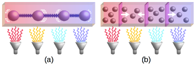
Figure 1: (a) Sketch of the linear chain of $N$ harmonic oscillators held in a temperature gradient: Each oscillator is coupled to an independent heat bath at temperature $T_{n}$, $n=0,...,N$ (in the picture $N$ =3). (b) Schematic interpretation in terms of sound propagation in a medium.

Here we analyze the energy repartition among the elastic modes of a harmonic chain held in temperature gradient, as sketched in Fig. 1(a). In a coarse-grained picture, the oscillator displacements can be thought of as the local strain of a (one-dimensional) elastic dispersive body, such that the model describes the damped propagation of thermal phonons (Fig. 1(b)). Our approach is fully analytic and provides an explicit expression for the energy repartition among the modes in terms of their effective temperatures $\mathcal{T}_{kk}$. Exemplifying our results for temperature profiles with a defined concavity, we show that $\mathcal{T}_{kk}$’s depend only on this concavity and on the boundary conditions of the system. A naive expectation could be that deviations from energy equipartition are to be anticipated at long wavelengths only, since local equilibrium conditions should hold at short scales. On the contrary, we find that both long and short wavelength modes can either heat up or cool down well beyond the average temperature. We also study a reverse-engineering approach in which the heat bath temperatures are inferred starting from a desired energy repartition.

II Model and general results

Consider a linear chain of $N+1$ equal oscillators located at positions $q_{n}$ ($n=0,1,\ldots,N$). Successive masses are connected through a harmonic potential of equilibrium length $l_{0}$. Each of them is in contact with a specific Langevin bath at temperature $T_{n}$ continuous , providing viscous damping with coefficient $\gamma$ and thermal noise $\xi_{n}$. Setting masses to unity, the equations of motion in the displacement coordinate $R_{n}\equiv q_{n}-n\,l_{0}$ read

$$\ddot{R}_{n} =-\gamma\dot{R}_{n}-\kappa\sum_{m=0}^{N}A_{nm}R_{m}+\xi_{n},$$ (1)

where $A_{nm}$ is a tridiagonal matrix accounting for first-neighbors interactions via the potential $\frac{\kappa}{2}(R_{m}-R_{m-1})^{2}$. In Eq. (1) the standard Gaussian white noise $\xi_{n}$ has an amplitude given by the fluctuation-dissipation theorem at the local temperature (in units of $k_{B}$):

$$\langle\xi_{m}(t)\,\xi_{n}(t^{\prime})\rangle=2\gamma\,T_{n}\;\delta(t-t^{\prime})\;\delta_{mn}.$$ (2)

In the following, we first consider the case of free boundary conditions ($A_{00}=A_{NN}=1$); fixed ($A_{00}=A_{NN}=0$) and mixed ($A_{00}=1$, $A_{NN}=0$) boundary conditions are discussed later in Appendix A. With free boundaries the matrix $A_{nm}$ is diagonalized by the linear transformation $\Phi^{-1}A\Phi$, with

$$\Phi^{-1}_{kn}=\frac{1}{N+1}\cos\left(\frac{k\pi}{N+1}\Big{(}n+\frac{1}{2}\Big{)}\right),$$ (3)

mapping the spatial coordinates $R_{n}$ into the coordinates of the normal modes $X_{k}\equiv\sum_{n}\Phi_{kn}^{-1}R_{n}$, for which

$$\ddot{X}_{k}=-\gamma\,\dot{X}_{k}-\omega_{k}^{2}\,X_{k}+\eta_{k},$$ (4)

where $\omega_{k}^{2}=4\kappa\,\sin^{2}\left(\frac{k\pi}{2(N+1)}\right)$ is the (squared) eigenfrequency of the $k$-th mode. In this dynamics, the only source of correlation between modes is contained in the transformed Gaussian white noises $\eta_{k}\equiv\sum_{n}\Phi_{kn}^{-1}\,\xi_{n}$,

$$\langle\eta_{k}(t)\,\eta_{k^{\prime}}(t^{\prime})\rangle=2\gamma\,\mathcal{T}_{kk^{\prime}}\,\delta(t-t^{\prime})/(N+1),$$ (5)

These correlation include a “temperature” matrix

$$\mathcal{T}_{kk^{\prime}}\equiv(N+1)\sum_{n=0}^{N}\Phi^{-1}_{kn}\,\Phi^{-1}_{k^{\prime}n}\,T_{n}\,,$$ (6)

which is certainly diagonal only in the equilibrium case $T_{n}=T\;\;\forall n$, where energy equipartition is recovered. In a nonequilibrium state, generated by heterogeneous bath-temperatures, the diagonal $\mathcal{T}_{kk}$ still encodes information about how energy is distributed among the modes. Non-zero off-diagonal $\mathcal{T}_{kk^{\prime}}$ emerge in connection with energy fluxes. To show this, we consider the average kinetic energy ($K_{k}$) and potential energy ($V_{k}$) of the $k$-th mode,

$$\ K_{k}\equiv(N+1)\,\langle\dot{X}_{k}^{2}\rangle\,(1-\delta_{k0}/2), V_{k}\equiv(N+1)\,\omega_{k}^{2}\,\langle X_{k}^{2}\rangle,$$

where expectation values $\langle\cdot\rangle$ are taken over different realizations of the thermal noise $\xi_{n}$. We get the variances $\langle X_{k}^{2}\rangle$, $\langle\dot{X}_{k}^{2}\rangle$ from the solution of Eq. (4) (Appendix B),

$$X_{k}(t) =\sum_{\alpha=1,2}\int_{-\infty}^{t}dt^{\prime}\frac{(-1)^{\alpha}}{\lambda_{k}^{1}-\lambda_{k}^{2}}e^{-\lambda_{k}^{\alpha}(t-t^{\prime})}\eta_{k}(t^{\prime}),$$ (7)

where $\lambda^{(\alpha)}_{k}$ with $\alpha=1,2$ are the roots of the characteristic equation for the unforced harmonic oscillator; namely, $\lambda^{(\alpha)}_{k}=-\frac{1}{2}[\gamma+(-1)^{\alpha}\sqrt{\gamma^{2}-4\,\omega_{k}^{2}}]$. For each mode $k$, both the average kinetic and potential energy turn out to coincide with one half of the mode temperature (Appendix B):

$$K_{k}^{X}=V_{k}^{X}={\cal T}_{kk}/2\quad(k\neq 0).$$ (8)

This relation establishes a form of energy equipartition between the conjugate variables of a single mode. Interestingly, from (6) and (3) one sees that ${\cal T}_{kk}$ does not depend on the details of both the harmonic interaction ($\kappa$) and the damping ($\gamma$). Therefore, the amount of energy stored in the $k$-th mode is directly determined by the choice of the bath temperature profile $T_{n}$, for given boundary conditions. Put in other words, properly designing thermal profiles it is in principle possible to enhance or reduce the thermal vibrations of specific modes. All these findings are confirmed by numerical integration of (1).

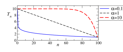
Figure 2: Heat-bath profiles utilized for exemplifying our results.

III Role of the boundary conditions

In the case of free boundaries, Eq. (6) gives

$${\cal T}_{kk}={\overline{T}}\,\left[1+\frac{\sum_{n=0}^{N}T_{n}\cos\left(\frac{2n+1}{N+1}\,k\pi\right)}{\sum_{m=0}^{N}T_{m}}\right]\;(k\neq 0),$$ (9)

where ${\overline{T}\equiv\sum_{n=0}^{N}T_{n}/(N+1)}$ is the average imposed temperature. The center-of-mass kinetic energy ${(N+1)\langle\dot{X_{0}}^{2}\rangle/2}$ is equal to ${\cal T}_{00}=\overline{T}$. Notice that Eq. (9) is valid in particular when $T_{n}$ corresponds to a self-consistent profile bolsterli_01 ; bonetto_01 ; dhar_06 . In (9) the energy stored by the mode $k$ under stationary nonequilibrium conditions emerges like a correction to the average temperature $\overline{T}$, which at most amounts to $\pm\overline{T}$. This correction can be viewed as a weighted average of a cosine function over the temperature profile: For parity, it vanishes for all temperature profiles which are odd with respect to $(N/2,\overline{T})$. The relevant physical consequence is that with free boundary conditions energy equipartition is extended to all nonequilibrium temperature profiles which are odd-symmetric with respect to $(N/2,\overline{T})$, like linear profiles. At variance, if the temperature profile has a definite upwards (downwards) concavity in the interval $[0,N]$, low- (high-) $k$ modes heat up and high- (low-) $k$ modes freeze down. We exemplify these findings assuming heat-bath temperatures $T_{n}=T_{0}+(n/N)^{\alpha}\,(T_{N}-T_{0})$ with $T_{0}=10$, $T_{N}=1$, and $N=99$ (see Fig. 2): $\alpha=1$ corresponds to a linear temperature profile, whereas $\alpha<1$ ($\alpha>1)$ corresponds to a profile with upwards (downwards) concavity. In Fig. 3(a) one finds the resulting $T_{kk}$ for free boundary conditions.

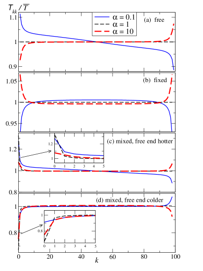
Figure 3: Modes normalized temperatures ${\cal T}_{kk}/\overline{T}$ calculated through Eqs. (9), (10), (11) for the heat-bath profiles mentioned earlier. The four panels refer to different boundary conditions: (a) free, (b) fixed, (c) mixed with free end hotter than the fixed end, and (d) vice versa. Insets enlarge the plots at low $k$’s.

Transport properties might depend crucially on the boundary conditions kundu_10 . We show that the latter strongly influences also the repartition of energy among the normal modes. For fixed boundary conditions, ${\cal T}_{kk}$ becomes (Appendix A)

$${\cal T}_{kk}=\frac{(N-1)\,{\overline{T}}}{N}\,\left[1-\frac{\sum_{n=1}^{N-1}T_{n}\cos\left(\frac{2n\,k}{N}\,\pi\right)}{\sum_{m=1}^{N-1}T_{m}}\right]$$ (10)

($0<k<N$), with $\overline{T}\equiv\sum_{n=1}^{N-1}T_{n}/(N-1)$. Fig. 3(b) shows the mode energy repartition for the same profiles $T_{n}$ used for open boundary conditions in Fig. 3(a). Notably, the low-$k$ behavior is inverted. For instance, while free boundaries enhance the long-wavelength energy storage for concave-up $T_{n}$, fixed boundaries do the opposite. Hence, if the aim were to store energy at low $k$’s, a convenient strategy would be to heat up the boundaries and cool down the middle of a free chain, and vice versa with a fixed chain.

For mixed boundaries in which we leave free the mass at $n=0$ and fix the mass at $n=N$ we have (Appendix A)

$${\cal T}_{kk}=\frac{2N\,{\overline{T}}}{2N+1}\,\left[1+\frac{\sum_{n=0}^{N-1}T_{n}\cos\left(\frac{(2n+1)\,(2k+1)}{2N+1}\,\pi\right)}{\sum_{m=0}^{N-1}T_{m}}\right]$$ (11)

($k<N$), with $\overline{T}\equiv\sum_{n=0}^{N-1}T_{n}/N$. Due to the broken symmetry upon profile reflection with respect to the vertical axis passing through $N/2$, in our exemplification we may distinguish two cases for each temperature profile: One in which the hotter temperatures are applied at the side of the free end in $n=0$ (as in Fig. 2) and one in which hot temperatures are applied at the side of the fixed mass in $n=N$ (perform the transformation $T_{n}\mapsto T_{N-n}$ to the profiles in Fig. 2). Results are respectively depicted in Fig. 3(c) and 3(d). In both cases, even the linear temperature profile does not lead to equipartition. From the plots one notices that low-$k$ modes store more energy if the free end is hotter. This alludes to suggestive implications: The mixed boundary is the case considered in Ref. conti_01 , where an experiment with a solid bar and a numerical study of an anharmonic chain displayed behaviors qualitatively consistent with that of Fig. 3(c). Our results thus suggest that the noise at lowest $k$’s would be lowered by letting the free end to float in a colder environment. This also points out a conceivable indication for reducing the measured thermal noise in experiments passible to schematizations analogous to those in Fig. 1.

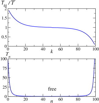
Figure 4: Reconstruction of the temperature profile (lower panel) through Eq. (12), starting from ${\cal T}_{kk}/\overline{T}$ displayed in the upper panel and $\overline{T}=5.5$.

IV Reverse engineering

The expression ${\cal T}_{kk}(T_{n})$ may be inverted, thus determining which heat-bath temperature profiles $T_{n}$ may correspond to a given mode energy repartition. For definiteness, let us focus on the case of free boundaries. Thanks to simple identities (Appendix C), the inversion of Eq. (9) gives

$$T_{n}+T_{N-n}=2\sum_{k=1}^{N}\cos\left(\frac{2n+1}{N+1}\,k\pi\right){\cal T}_{kk}+2\overline{T}.$$ (12)

Notice that, given ${\cal T}_{kk}$, the temperature profile $T_{n}$ is not uniquely identified. In fact, the relation ${\cal T}_{kk}(T_{n})$ is many-to-one – for instance, already on the basis of symmetry one can figure out that temperature profiles $T_{n},\;T^{\prime}_{n}$ related by the transformation $T^{\prime}_{n}=T_{N-n}$ produce the same energy repartition $T_{kk}$. In the lower panel of Fig. 4 we display a profile reconstruction originated from the specific choice for ${\cal T}_{kk}$ reported in the upper one. For simplicity, we complemented Eq. (12) with the condition $T_{n}=T_{N-n}$; this means, in particular, $T_{0}=T_{N}$. Our example points out that in principle it is possible to design heat-bath temperature profiles so that the energy stored in the normal modes of the chain is arbitrarily distributed in the range $[0,2\overline{T}]$, consistently with the condition $\sum_{k=1}^{N}{\cal T}_{kk}=N\,\overline{T}$.

V Power spectrum

To show that $\mathcal{T}_{kk}$ also encodes the dynamics of fluctuations, we compute the power spectrum $S(\omega)$ of the chain length $R_{N}-R_{0}+N\,l_{0}$ in the frequency domain, a quantity typically monitored in experiments conti_01 . According to the Wiener-Khinchin theorem kuboII , under stationary conditions $S(\omega)$ is given by the Fourier transform of the chain length’s autocorrelation function. Referring again to free boundary conditions, in terms of normal modes we have ${R_{N}-R_{0}=\sum_{k=1}^{N}(\Phi_{Nk}-\Phi_{0k})X_{k}}$. Hence (Appendix D),

$$S(\omega) =\!\frac{2\gamma}{N+1}\sum_{k,k^{\prime}=1}^{N}\frac{\;(\Phi_{Nk}-\Phi_{0k})\;(\Phi_{Nk^{\prime}}-\Phi_{0k^{\prime}})\;\mathcal{T}_{k{k^{\prime}}}}{({\omega_{k}^{2}}-\omega^{2}-\mathrm{i}\gamma\omega)\;({\omega_{k^{\prime}}^{2}}-\omega^{2}+\mathrm{i}\gamma\omega)}$$ (13)

$$\simeq\frac{16\gamma}{N+1}\sum_{\textrm{odd}\;k}\frac{\cos^{2}\left(\frac{k}{2(N+1)}\,\pi\right)\,{\cal T}_{kk}}{(\omega_{k}^{2}-\omega^{2})^{2}+\gamma^{2}\,\omega^{2}}$$ (14)

($\omega\neq 0$), where even modes do not contribute owing to the symmetry of the boundaries. Eq. (14) neglects the cross-correlations between modes at different $k$. Such cross-correlation terms are instead responsible for the heat flux along the chain, $J_{n}=l_{0}\,\kappa\,\langle\dot{R}_{n}R_{n-1}\rangle$ lepri_03 . In terms of normal modes we have (Appendix D) in fact

$$J_{n}=- \frac{\mathrm{i}\,l_{0}\,\kappa}{(2\pi)^{2}}\;\frac{2\gamma}{N+1}\sum_{k\neq k^{\prime}}\Phi_{nk}\Phi_{n-1,k^{\prime}}\;\mathcal{T}_{k{k^{\prime}}}\times$$

$$\times\int\text{d}\omega\,\;\frac{\omega}{({\omega_{k}^{2}}-\omega^{2}-\mathrm{i}\gamma\omega)\;({\omega_{k^{\prime}}^{2}}-\omega^{2}+\mathrm{i}\gamma\omega)}$$ (15)

($0<n<N$). We have checked that the contribution of terms with $k^{\prime}\neq k$ in Eq. (13) can only be appreciated in proximity of the negative peaks of the power spectrum, away from the resonances $\omega_{k}$.

VI Conclusions

In summary, our analytic study of energy repartition in a harmonic chain in contact with independent heat baths shows that both long and short wavelength modes may have energies which deviate significantly from the level expected if equipartition were to hold. This enhanced or reduced storage of energy depends critically on the shape of the temperature profile and on the boundary conditions. Other dynamical properties, such as the damping or the elastic coupling, are instead totally irrelevant. Thus, for a generic harmonic chain, information encoded in the temperature profile is mapped into a sequence of vibrational mode temperatures, which in turn shape the power spectrum of the chain length. Investigations about the influence on the above picture of nonlinearities originating thermo-mechanical couplings, is the next important step.

Appendix A Boundary conditions

A.1 Free boundary conditions

In the case of free boundary conditions with $N+1$ oscillators the Laplacian matrix is

$$A\equiv\left(A_{nm}\right)_{n,m=0,1,\ldots,N}\equiv\left(\begin{array}[]{cccccc}+1&-1&0&\cdots&&0\\ -1&+2&-1&\ddots&&\vdots\\ 0&-1&\ddots&\ddots&&\\ \vdots&\ddots&\ddots&&-1&0\\ &&&-1&+2&-1\\ 0&\cdots&&0&-1&+1\end{array}\right)\;,$$ (16)

which is diagonalized by the linear transformation $\Phi^{-1}A\Phi$, with

$$\Phi_{nk}=\left\{\begin{array}[]{ll}1&k=0\\ \sqrt{2}\cos\left(\frac{(2n+1)\;k}{2(N+1)}\;\pi\right)&k\neq 0\end{array}\right.\;,$$ (17)

$$\Phi^{-1}=\frac{\Phi^{t}}{N+1}\;.$$ (18)

It is straightforward to see that the definition

$$\mathcal{T}_{kk}\equiv(N+1)\sum_{n=0}^{N}\Phi^{-1}_{kn}\,\Phi^{-1}_{kn}\,T_{n}$$ (19)

leads to

$${\cal T}_{kk}={\overline{T}}\,\left[1+\frac{\sum_{n=0}^{N}T_{n}\cos\left(\frac{2n+1}{N+1}\,k\pi\right)}{\sum_{m=0}^{N}T_{m}}\right]\quad(0<k\leq N)$$ (20)

and ${\cal T}_{00}=\overline{T}\equiv\sum_{n=0}^{N}T_{n}/(N+1)$. Notice that $\sum_{n=0}^{N}\cos\left(\frac{2n+1}{N+1}\,k\pi\right)=0$, so that at equilibrium, $T_{n}=\overline{T}\;\forall n$, we recover $\mathcal{T}_{kk}=\overline{T}\;\forall k$.

A.2 Fixed boundary conditions

In the case of fixed boundary we can stick to our notations by fixing the two masses at the border. The number of oscillators becomes $N-1$, and the Laplacian matrix reads

$$A\equiv\left(A_{nm}\right)_{n,m=0,1,\ldots,N}\equiv\left(\begin{array}[]{cccccc}0&0&0&\cdots&&0\\ 0&+2&-1&\ddots&&\vdots\\ 0&-1&\ddots&\ddots&&\\ \vdots&\ddots&\ddots&&-1&0\\ &&&-1&+2&0\\ 0&\cdots&&0&0&0\end{array}\right)\;,$$ (21)

which now is diagonalized by

$$\Phi_{nk}=\left\{\begin{array}[]{ll}\sqrt{N}&(n,k)=(0,0)\;\textrm{or}\\ &(n,k)=(N,N)\\ 0&(0<n\leq N,k=0)\;\textrm{or}\\ &(0<n\leq N,k=N)\\ \sqrt{2}\sin\left(\dfrac{n\;k}{N}\;\pi\right)&\textrm{otherwise}\end{array}\right.\;,$$ (22)

$$\Phi^{-1}=\frac{\Phi^{t}}{N}\;.$$ (23)

Also in this case it is straightforward to show that

$${\cal T}_{kk}=\frac{(N-1)\,{\overline{T}}}{N}\,\left[1-\frac{\sum_{n=1}^{N-1}T_{n}\cos\left(\frac{2n\,k}{N}\,\pi\right)}{\sum_{m=1}^{N-1}T_{m}}\right]$$ (24)

$$\qquad(0<k<N),$$

with $\overline{T}\equiv\sum_{n=1}^{N-1}T_{n}/(N-1)$. We have $\sum_{n=1}^{N-1}\cos\left(\frac{2n\,k}{N}\,\pi\right)=-1$, so that at equilibrium we again recover $\mathcal{T}_{kk}=\overline{T}\;\forall k$.

A.3 Mixed boundary conditions

In the case of mixed boundary we fix only the mass at $n=N$. The number of oscillators becomes $N$ and the Laplacian matrix is

$$A\equiv\left(A_{nm}\right)_{n,m=0,1,\ldots,N}\equiv\left(\begin{array}[]{cccccc}+1&-1&0&\cdots&&0\\ -1&+2&-1&\ddots&&\vdots\\ 0&-1&\ddots&\ddots&&\\ \vdots&\ddots&\ddots&&-1&0\\ &&&-1&+2&0\\ 0&\cdots&&0&0&0\end{array}\right)\;,$$ (25)

which is diagonalized by the linear transformation $\Phi^{-1}A\Phi$ with

$$\Phi_{nk}=\left\{\begin{array}[]{l}\sqrt{\frac{2N+1}{2}}\qquad(n,k)=(N,N)\\ 0\qquad\quad\qquad(n=N,0\leq k<N)\;\textrm{or}\\ \ \qquad\quad\qquad(0\leq n<N,k=N)\\ \sqrt{2}\cos\left(\dfrac{(2n+1)\;(2k+1)}{2(2N+1)}\;\pi\right)\quad\textrm{otherwise}\end{array}\right.\;,$$ (26)

$$\Phi^{-1}=\frac{2\,\Phi^{t}}{2N+1}\;.$$ (27)

As for the previous cases, it is easy to prove that

$${\cal T}_{kk}=\frac{2N\,{\overline{T}}}{2N+1}\,\left[1+\frac{\sum_{n=0}^{N-1}T_{n}\cos\left(\frac{(2n+1)\,(2k+1)}{2N+1}\,\pi\right)}{\sum_{m=0}^{N-1}T_{m}}\right]$$ (28)

$$(0\leq k<N),$$

with $\overline{T}\equiv\sum_{n=0}^{N-1}T_{n}/N$. In this case $\sum_{n=0}^{N-1}\cos\left(\frac{(2n+1)\,(2k+1)}{2N+1}\,\pi\right)=1/2$, and again one recovers $\mathcal{T}_{kk}=\overline{T}\;\forall k$ at equilibrium.

Appendix B Energy repartition among the modes

Equation

$$\ddot{X}_{k}=-\gamma\,\dot{X}_{k}-\omega_{k}^{2}\,X_{k}+F_{k}$$ (29)

is a first-order linear differential equation in the vector $\mathbf{Y}_{k}\equiv(X_{k},\dot{X}_{k})$. Its stationary solution is formally given by

$$\mathbf{Y}_{k}(t)=\int_{-\infty}^{t}\;dt^{\prime}\exp[(t-t^{\prime})\mathbf{\Lambda}_{k}]\cdot\mathbf{F}_{k}(t^{\prime}),$$ (30)

with the definitions

$$\mathbf{\Lambda}_{k}=\begin{pmatrix}0&1\\ -\omega_{k}^{2}&-\gamma\\ \end{pmatrix}, \mathbf{F}_{k}=\begin{pmatrix}0\\ F_{k}\\ \end{pmatrix}.$$ (31)

The matrix exponential in Eq. (30) is computed by diagonalizing $\mathbf{\Lambda}_{k}$. Its eigenvalues $\lambda^{\scriptscriptstyle{1,2}}_{k}$ are the two solutions of the characteristic equation for the unforced harmonic oscillator, namely

$$\lambda^{\alpha}_{k}=\frac{1}{2}\left(-\gamma+(-1)^{\alpha-1}\sqrt{\gamma^{2}-4\,\omega_{k}^{2}}\right), \alpha=1,2\,.$$ (32)

Therefore, from the solutions

$$X_{k}(t) = \sum_{\alpha=1,2}\int_{-\infty}^{t}\,dt^{\prime}\,A_{k}^{\alpha}\exp(-\lambda_{k}^{\alpha}(t-t^{\prime}))\,F_{k}(t^{\prime}),\qquad$$ (33)

$$\dot{X}_{k}(t) = \sum_{\alpha=1,2}\int_{-\infty}^{t}\,dt^{\prime}\,B_{k}^{\alpha}\exp(-\lambda_{k}^{\alpha}(t-t^{\prime}))\,F_{k}(t^{\prime}),\qquad$$ (34)

with

$$A^{1}_{k} = \frac{1}{\lambda_{k}^{2}-\lambda_{k}^{1}}=-A_{k}^{2},$$ (35)

$$B^{1}_{k} = -\frac{\lambda_{k}^{1}}{\lambda_{k}^{2}}B^{2}_{k}=\lambda_{k}^{1}A_{k}^{2},$$ (36)

we can evaluate the stationary equal-time correlations

$$\langle X_{k}X_{k^{\prime}}\rangle=2\zeta\mathcal{T}_{kk^{\prime}}\sum_{\alpha,\beta=1,2}\frac{A_{k}^{\alpha}A_{k^{\prime}}^{\beta}}{\lambda_{k}^{\alpha}+\lambda_{k^{\prime}}^{\beta}},$$ (37)

$$\langle\dot{X}_{k}\dot{X}_{k^{\prime}}\rangle=2\zeta\mathcal{T}_{kk^{\prime}}\sum_{\alpha,\beta=1,2}\frac{B_{k}^{\alpha}B_{k^{\prime}}^{\beta}}{\lambda_{k}^{\alpha}+\lambda_{k^{\prime}}^{\beta}}.$$ (38)

For the average kinetic and potential energy per mode,

$$K_{k} \equiv (N+1)\,\langle\dot{X}_{k}^{2}\rangle\,(1-\delta_{k0}/2),$$ (39)

$$V_{k} \equiv (N+1)\,\omega_{k}^{2}\,\langle X_{k}^{2}\rangle,$$ (40)

we thus obtain the basic result

$$K_{k}^{X}=V_{k}^{X}={\cal T}_{kk}/2\quad(k\neq 0).$$ (41)

Appendix C Reconstructing the temperature profile

Expressing the cosine in complex notation it is easy to prove the following identities:

$$\sum_{k=1}^{N}\cos\left(\frac{(2m+1)\,k}{N+1}\,\pi\right)\;\cos\left(\frac{(2n+1)\,k}{N+1}\,\pi\right)=$$

$$\qquad=\frac{N+1}{2}\left(\delta_{m\,n}+\delta_{m\,N-m}\right)-1,$$ (42)

$$\sum_{k=1}^{N}\cos\left(\frac{(2m+1)\,k}{N+1}\,\pi\right)=0.$$ (43)

Hence, from Eq. (6) we obtain

$$\sum_{k=1}^{N}\cos\left(\frac{(2m+1)\,k}{N+1}\,\pi\right)\;{\cal T}_{kk}=$$ (44)

$$\qquad=\sum_{k=1}^{N}\cos\left(\frac{(2m+1)\,k}{N+1}\,\pi\right){\overline{T}}$$

$$\qquad\qquad\times\,\left[1+\frac{\sum_{n=0}^{N}T_{n}\cos\left(\frac{2n+1}{N+1}\,k\pi\right)}{\sum_{m=0}^{N}T_{m}}\right],$$ (45)

or

$$T_{n}+T_{N-n}=2\sum_{k=1}^{N}\cos\left(\frac{2n+1}{N+1}\,k\pi\right){\cal T}_{kk}+2\overline{T}.$$ (46)

Appendix D Spectral density

According to the Wiener-Khinchin theorem kuboII , under stationary conditions the spectral density $S(\omega)$ of the chain length $R_{N}-R_{0}+N\,l_{0}$ is given by

$$S(\omega)=\int{\rm d}\tau\;\mathrm{e}^{\mathrm{i}\omega t}\left\langle\;\left[R_{N}(t_{0})-R_{0}(t_{0})\right]\;\left[R_{N}(t_{0}+\tau)-R_{0}(t_{0}+\tau)\right]\right\rangle+2\pi\,N^{2}\,l_{0}^{2}\;\delta(\omega)$$ (47)

We have

$$R_{N}(t)-R_{0}(t)=\sum_{k=1}^{N}(\Phi_{Nk}-\Phi_{0k})\;X_{k}(t),$$ (48)

so that

$$S(\omega)=\sum_{k,k^{\prime}=1}^{N}\;(\Phi_{Nk}-\Phi_{0k})\;(\Phi_{Nk^{\prime}}-\Phi_{0k^{\prime}})\int{\rm d}\tau\;\mathrm{e}^{\mathrm{i}\omega t}\left\langle\;X_{k}(t_{0})\;X_{k^{\prime}}(t_{0}+\tau)\right\rangle+2\pi\,N^{2}\,l_{0}^{2}\;\delta(\omega)$$ (49)

We indicate the Fourier transform of a generic function $h(t)$ as $\displaystyle{\widehat{h}(\omega)\equiv\int{\rm d}t\,\mathrm{e}^{\text{i}\omega t}\,h(t)}$, and denote its complex conjugate as $\widehat{h}^{*}(\omega)$. The Fourier transform of Eq. (4) gives

$$-\omega^{2}\widehat{X}_{k}(\omega)=\mathrm{i}\omega\gamma\widehat{X}_{k}(\omega)-{\omega_{k}^{2}}\widehat{X}_{k}(\omega)+\widehat{\eta}_{k}(\omega).$$ (50)

Solving for $\widehat{X}_{k}(\omega)$ and using

$$\langle\eta_{k}(t)\,\eta_{k^{\prime}}(t^{\prime})\rangle=2\gamma\,\mathcal{T}_{kk^{\prime}}\,\delta(t-t^{\prime})/(N+1)$$ (51)

we obtain, for $\omega\neq 0$,

$$S(\omega)=\frac{2\gamma}{N+1}\sum_{k,k^{\prime}=1}^{N}\frac{\;(\Phi_{Nk}-\Phi_{0k})\;(\Phi_{Nk^{\prime}}-\Phi_{0k^{\prime}})\;\mathcal{T}_{k{k^{\prime}}}}{({\omega_{k}^{2}}-\omega^{2}-\mathrm{i}\gamma\omega)\;({\omega_{k^{\prime}}^{2}}-\omega^{2}+\mathrm{i}\gamma\omega)}.$$ (52)

The local heat flux $J_{n}$ along the chain lepri_03 is given by

$$J_{n}=l_{0}\,\kappa\;{\left<\dot{R}_{n}R_{n-1}\right>}\qquad(0<n<N).$$ (53)

In terms of normal modes the local heat flux becomes

$$J_{n}=l_{0}\,\kappa\;\sum_{k\neq k^{\prime}}\Phi_{nk}\,\Phi_{n-1k^{\prime}}\;{\left<\dot{X}_{k}X_{k^{\prime}}\right>}.$$ (54)

Indeed, stationarity implies ${\left<\dot{X}_{k}X_{k}\right>}=0$ for equal-time averages. We then have

$${\left<\dot{X}_{k}X_{k^{\prime}}\right>} =\frac{1}{(2\pi)^{2}}\int{\rm d}\omega\int{\rm d}\omega^{\prime}(-\text{i}\omega)\;\mathrm{e}^{-\text{i}\omega t}\;\mathrm{e}^{\text{i}\omega^{\prime}t}{\left<\widehat{X}_{k}(\omega)\;\widehat{X}^{*}_{k^{\prime}}(\omega^{\prime})\right>}$$ (55)

$$=\frac{1}{(2\pi)^{2}}\int{\rm d}\omega\int{\rm d}\omega^{\prime}(-\text{i}\omega)\;\mathrm{e}^{-\text{i}\omega t}\;\mathrm{e}^{\text{i}\omega^{\prime}t}\;\frac{2\gamma}{N+1}\;\frac{\;\mathcal{T}_{k{k^{\prime}}}}{({\omega_{k}^{2}}-\omega^{2}-\mathrm{i}\gamma\omega)\;({\omega_{k^{\prime}}^{2}}-\omega^{\prime 2}+\mathrm{i}\gamma\omega^{\prime})}\;\delta(\omega-\omega^{\prime})$$ (56)

$$=-\frac{\text{i}}{(2\pi)^{2}}\;\frac{2\gamma\;\mathcal{T}_{k{k^{\prime}}}}{N+1}\int{\rm d}\omega\;\frac{\omega}{({\omega_{k}^{2}}-\omega^{2}-\mathrm{i}\gamma\omega)\;({\omega_{k^{\prime}}^{2}}-\omega^{2}+\mathrm{i}\gamma\omega)}.$$ (57)

Putting things together we obtain

$$J_{n}=-\frac{\mathrm{i}\,l_{0}\,\kappa}{(2\pi)^{2}}\;\frac{2\gamma}{N+1}\sum_{k\neq k^{\prime}}\Phi_{nk}\Phi_{n-1,k^{\prime}}\;\mathcal{T}_{k{k^{\prime}}}\int\text{d}\omega\,\;\frac{\omega}{({\omega_{k}^{2}}-\omega^{2}-\mathrm{i}\gamma\omega)\;({\omega_{k^{\prime}}^{2}}-\omega^{2}+\mathrm{i}\gamma\omega)}\qquad(0<n<N).$$ (58)

References

- (1) J. M. Ortiz de Zárate and J. V. Sengers, Hydrodynamic Fluctuations in Fluids and Fluid Mixtures, Elsevier, New York (2006).
- (2) R. Schmitz, Fluctuations in Nonequilibrium Fluids, Physics Reports 171, 1 (1988).
- (3) P. N. Segrè, R.W. Gammon, J. V. Sengers, and B. M. Law, Rayleigh scattering in a liquid far from thermal equilibrium, Phys. Rev. A 45, 714 (1992).
- (4) W. B. Li, K. J. Zhang, J. V. Sengers, R. W. Gammon, and J. M. Ortiz de Zárate, Concentration Fluctuations in a Polymer Solution under a Temperature Gradient, Phys. Rev. Lett. 81, 5580 (1998).
- (5) C. J. Takacs, A. Vailati, R. Cerbino, S. Mazzoni, M. Giglio, and D. S. Cannell, Thermal Fluctuations in a Layer of Liquid Subjected to Temperature Gradients with and without the Influence of Gravity, Phys. Rev. Lett. 106, 244502 (2011).
- (6) A. C. Bleszynski-Jayich, W. E. Shanks, and J. G. E. Harris, Noise thermometry and electron thermometry of a sample-on-cantilever system below 1Kelvin, Applied Physics Letters 92, 013123 (2008).
- (7) L. Conti, M. Bonaldi, L. Rondoni, RareNoise: non-equilibrium effects in detectors of gravitational waves , Cl. Quant. Grav. 24, 084032 (2010).
- (8) L. Conti, P. De Gregorio, G. Karapetyan, C. Lazzaro, M. Pegoraro, M. Bonaldi, L. Rondoni, Effects of breaking vibrational energy equipartition on measurements of temperature in macroscopic oscillators subject to heat flux, J. Stat. Mech. P12003 (2013).
- (9) F. Aguilar Sandoval, M. Geitner, E. Bertin, L. Bellon, Resonance frequency shift of strongly heated micro-cantilevers J. Appl. Phys. 117, 234503 (2015)
- (10) In order to identify low frequency fluctuations with low wavenumber fluctuations, one has to assume a monotonic dispersion relation, which is the case for acoustic phonons.
- (11) S. Lepri, R. Livi, and A. Politi Heat Conduction in Chains of Nonlinear Oscillators, Phys. Rev. Lett. 78, 1896 (1997)
- (12) S. Lepri, R. Livi, and A. Politi Thermal conduction in classical low-dimensional lattices, Phys. Rep. 377, 1 (2003).
- (13) A. Dhar, Heat transport in low-dimensional systems Adv. in Phys. 57, 457 (2008).
- (14) M. Bolsterli, M. Rich, W. M. Visscher, Simulation of Nonharmonic Interactions in a Cristal by Self-Consistent Reservoirs, Phys. Rev. A 1, 1086 (1970).
- (15) F. Bonetto, J. L. Lebowitz, J. Lukkarinen, Fourier’s Law for a Harmonic Crystal with Self-Consistent Stochastic Reservoirs, J. Stat. Phys. 116, 783 (2004).
- (16) D. Dhar and D. Roy, Heat Transport in Harmonic Lattices, J. Stat. Phys. 125, 801 (2006).
- (17) E. Pereira and R. Falcao, Normal Heat Conduction in a Chain with a Weak Interparticle Anharmonic Potential, Phys. Rev. Lett. 96, 100601 (2006).
- (18) H.C. Fogedby and A. Imparato, Heat fluctuations and fluctuation theorems in the case of multiple reservoirs, J. Stat. Mech. P11011 (2014).
- (19) F. Nicacio, A. Ferraro, A. Imparato, M. Paternostro, and F. L. Semião, Thermal transport in out-of-equilibrium quantum harmonic chains, Phys. Rev. E 91, 042116 (2015).
- (20) K. Somiya, Detector configuration of KAGRA - the Japanese cryogenic gravitational-wave detector Class. Quant. Grav. 29 124007 (2012).
- (21) This can be viewed as a simplified description of a continuous background temperature field as long as the characteristic length scale of the temperature variations are large with respect to the typical fluctuations of the oscillator positions, i.e. .
- (22) A. Kundu, A. Chaudhuri, D. Roy, A. Dhar, J. L. Lebowitz, and H. Spohn, Heat conduction and phonon localization in disordered harmonic crystals, Europhys. Lett. 90, 40001 (2010).
- (23) See, e.g., M. Toda, N. Saito, and R. Kubo, Statistical Physics II: Nonequilibrium Statistical Mechanics, (Springer Series in Solid-State Sciences 1991).