Fluctuating volume–current formulation of electromagnetic fluctuations in inhomogeneous media: incandecence and luminescence in arbitrary geometries

Abstract

We describe a fluctuating volume–current formulation of electromagnetic fluctuations that extends our recent work on heat exchange and Casimir interactions between arbitrarily shaped homogeneous bodies [Phys. Rev. B. 88, 054305] to situations involving incandescence and luminescence problems, including thermal radiation, heat transfer, Casimir forces, spontaneous emission, fluorescence, and Raman scattering, in inhomogeneous media. Unlike previous scattering formulations based on field and/or surface unknowns, our work exploits powerful techniques from the volume–integral equation (VIE) method, in which electromagnetic scattering is described in terms of volumetric, current unknowns throughout the bodies. The resulting trace formulas (boxed equations) involve products of well-studied VIE matrices and describe power and momentum transfer between objects with spatially varying material properties and fluctuation characteristics. We demonstrate that thanks to the low-rank properties of the associated matrices, these formulas are susceptible to fast-trace computations based on iterative methods, making practical calculations tractable. We apply our techniques to study thermal radiation, heat transfer, and fluorescence in complicated geometries, checking our method against established techniques best suited for homogeneous bodies as well as applying it to obtain predictions of radiation from complex bodies with spatially varying permittivities and/or temperature profiles.

I Introduction

Quantum and thermal fluctuations of charges give rise to a wide range of electromagnetic phenomena; these include luminescence from active media, e.g. fluorescence and spontaneous emission Siegman (1989); Agarwal (1974); Le Ru and Etchegoin (2008), the finite linewidth of lasers near threshold Gordon et al. (1955); Matloob et al. (1997), thermal radiation and heat transfer from hot objects Polder and Van Hove (1971); Joulain et al. (2005); Chen (2005); Carey et al. (2006); Fu and Zhang (2006); Volokitin and Persson (2007); Zhang (2007); Basu et al. (2009); Otey et al. (2014), and dispersive interactions (Casimir forces) between nearby surfaces Casimir and Polder (1948); Casimir (1948); Buhmann and Welsch (2007); Genet et al. (2008); Bordag et al. (2009); Rodriguez et al. (2011a); Rodriguez et al. (2014). Fluctuation-driven effects are not only responsible for many naturally occurring processes but are also poised to take an increasingly active role in emerging nanotechnologies Zhang (2007); Basu et al. (2009), spurring interest in the study and engineering of complex shapes that could dramatically alter their behavior Otey et al. (2014); Rodriguez et al. (2014). Although rooted in similar principles, the physical mechanisms behind each of these processes vary considerably, leading to theoretical descriptions that differ both in their formulation and implementation. Ultimately, however, all such calculations reduce to a series of classical scattering problems Khanert (2003); Johnson (2011) that until recently remained largely specialized to situations involving simple, high–symmetry geometries, e.g. planar and spherical objects.

In this manuscript, we present a framework for the general-purpose calculation of many different incandescence and luminescence processes, including fluorescence, spontaneous emission, thermal radiation, heat transfer, and Casimir forces in arbitrary geometries. In particular, we derive a fluctuating volume–current (FVC) formulation of electromagnetic fluctuations that exploits techniques from the volume–integral equation (VIE) formulation of electromagnetic scattering Chew et al. (2001a); Polimeridis et al. (2014) and which expands the range and validity of current methods to situations involving inhomogeneous media. Although FVC is similar in spirit to our previous fluctuating surface–current (FSC) methods Rodriguez et al. (2013); Rodriguez et. al. (2013), unlike FSC our new approach is not limited to piecewise-homogeneous objects. Here, the unknowns are volume currents within objects rather than surface currents as in FSC, and can therefore easily handle more complex structures, including inhomogeneous bodies with temperature gradients or spatially varying permittivities. In contrast to recently developed scattering-matrix methods Lambrecht et al. (2006); Milton and Wagner (2008); Rahi et al. (2009); Bimonte (2009); Biehs et al. (2011); Guérout et al. (2012); Messina and Antezza (2011); Kruger et al. (2011); Otey and Fan (2011); Golyk et al. (2012); Kruger et al. (2012); Marachevsky (2012); Lussange et al. (2012), the FVC and FSC methods do not require a separate basis of incoming/outgoing wave solutions to be selected (a potentially difficult task in geometries involving interleaved objects or complex structures favoring nonuniform spatial resolution), although VIE can be used to compute the scattering matrix if desired. We show that regardless of which quantity is computed, the final expressions for power and momentum transfer are based on simple trace formulas involving well-studied VIE and current–current correlation matrices that encode the spectral properties of fluctuating sources. We find that while the number of VIE unknowns is large compared to scattering or FSC formulations, the associated VIE matrices admit low-rank approximations that turn out to significantly reduce the complexity of trace evaluations, making practical calculations tractable. We validate the FVC method by checking its predictions against known solutions for homogeneous objects and then apply it to calculate thermal radiation, heat transfer, and fluorescence from compact objects (spheres, ellipsoids, and cubes) with spatially varying permittivities and temperature gradients. The same trace formulas can be readily adapted to obtain the angular distribution of far-field radiation, which we illustrate by providing new predictions of directional emission from inhomogeneous objects. the As explained below, while VIE methods can be applied to arbitrary geometries, they are particularly advantageous in situations where object sizes are on the order of (or smaller) than the relevant wavelengths, providing a useful complement to well-established techniques better suited for the study of arbitrary geometries with lengthscales that are large or small compared to the relevant electromagnetic wavelengths, e.g. proximity approximations Bordag et al. (2009); Sasihithlu and Narayanaswamy (2013).

Electromagnetic fluctuation phenomena can be roughly divided into two categories: incandescence and luminescence problems. Incandescence refers to electromagnetic radiation from objects generated by the quantum and thermal motion of charged particles in matter, whereas luminescence refers to incoherent emission of light from non-thermal sources. The oldest and most well-studied manifestation of incandescence is the familiar glow of objects—thermal radiation—that occurs when an object is heated above the temperature of its surrounding environment Reif (1965); Landau and Lifshitz (1980). Although Planck’s law was not more than a century ago at the center of vigorous controversy which helped establish the foundations of quantum mechanics Planck (1901), much of our recent interest in this phenomenon spawns from its profound impact on energy and related nanotechnologies. Interest in complex designs is also fueled by our increasing ability to engineer selective and even dynamically tunable emitters and detectors at wavelengths for which there is currently a lack of coherent sources Greffet et al. (2001); Laroche et al. (2006a); Zhang (2007); Schuller et al. (2009); Liu et al. (2011); Inoue et al. (2014), in addition to solar-energy harvesting applications Rephaeli and Fan (2009); Sergeant et al. (2010); Rinnerbauer et al. (2012); Gan et al. (2013); Lenert et al. (2014). In addition to radiation, fluctuations can also mediate heat exchange Polder and Van Hove (1971); Pendry (1999); Chen (2005) and interactions Casimir and Polder (1948); Joulain et al. (2005); Dalvit et al. (2011); Reid et al. (2013); Rodriguez et al. (2014) (known as Casimir forces) between objects—unlike heat exchange, Casimir interactions persist even at equilibrium and are known to arise primarily due to contributions of quantum rather than finite-temperature fluctuations. One fundamental distinction between “near-field” effects (between objects at wavelength-scale separations or less) and the more familiar “far-field” phenomena (separations $\gg$ wavelength) is that the former can be significantly enhanced by the contributions of evanescent waves Rytov et al. (1989); Polder and Van Hove (1971); Loomis and Maris (1994); Pendry (1999), growing in a power-law fashion with decreasing object separations. As a result, the heat transfer between real materials can exceed the predictions of the Planck blackbody law by orders of magnitude Basu et al. (2009) and quantum forces can even reach atmospheric pressures at nanometric lengthscales Rodriguez et al. (2014), motivating interest in complex designs that can be tailored for various applications, including thermophotovoltaic energy conversion Pan et al. (2000); Laroche et al. (2006b); Messina and Ben-Abdallah (2013); Ilic et al. (2012), nanoscale cooling Tschikin et al. (2012); St-Gelais et al. (2014), and MEMS design. Serry et al. (1998); Chan et al. (2001); DelRio et al. (2005)

Until very recently, however, calculations and experiments remained focused on planar structures and simple approximations thereof Mulet et al. (2002); Joulain et al. (2005); Chen (2005); Carey et al. (2006); Fu and Zhang (2006); Volokitin and Persson (2007); Zhang (2007); Basu et al. (2009); Otey et al. (2014). Since all such thermal effects arise due to the presence of fluctuating current sources, from the perspective of calculations their descriptions reduce to a series of classical scattering calculations involving fields due to currents Johnson (2011); Otey et al. (2014), the spectral characteristics of which are related to the underlying physical means of excitations. In the case of incandescence, they are determined by the thermal and dissipative properties of materials via the well-known fluctuation–dissipation theorem (FDT) Eckhardt (1984); Landau et al. (1960). Naively, this involves repeated calculations of electromagnetic Green’s functions throughout the bodies, which can prove prohibitive for complex objects where the latter must be computed numerically, especially due to the broad bandwidth associated with thermal fluctuations, but it turns out that more sophisticated formulations exist Rodriguez et al. (2014); Otey et al. (2014). These include time- and frequency-domain methods where the power transfer or force on an object is obtained via integrals of the flux or Maxwell stress tensor, or equivalently electromagnetic Green’s functions, along some arbitrary surface enclosing the body Narayanaswamy and Chen (2008); Rodriguez et al. (2009); McCauley et al. (2010); Xiong et al. (2010); Otey and Fan (2011); Rodriguez et al. (2011b); Narayanaswamy and Zheng (2014); Liu and Shen (2013). Recent techniques forgo surface integrations altogether in favor of unfamiliar but more efficient expressions involving traces of either scattering Biehs et al. (2008); Bimonte (2009); Messina and Antezza (2011); McCauley et al. (2012); Guérout et al. (2012); Marachevsky (2012); Kruger et al. (2012); Golyk et al. (2012) or boundary-element Rodriguez et al. (2013); Rodriguez et. al. (2013); Rodriguez et al. (2012) matrices. Regardless of the choice of unknowns, in practical implementations the latter are expanded in terms of either delocalized spectral bases (e.g. Fourier or Mie series) best suited for high–symmetry geometries, or geometry-agnostic localized bases (piecewise polynomial “element” functions) defined on meshes or grids and applicable to arbitrary objects Johnson (2011). While there has been much progress so far, these methods have yet to be generalized to handle structures with temperature gradients or varying permittivities.

Temperature gradients can arise for instance due to the interplay of phonon and photon transport Cahill et al. (2002, 2003), such as in heterogeneous structures with disparate thermal conductivities, including chalcogenide/metal interfaces Xiong et al. (2009); Liang et al. (2012) or quartz-platium-polymer structures Fenwick et al. (2009), or in graphene-based devices Islam et al. (2013). Temperature gradients have also been observed in atomic force microscopes King et al. (2013); Biehs et al. (2012) and nanowires Yeo et al. (2014), as well as in situations involving irradiated particles immersed in fluids Merabia et al. (2009); Baffou et al. (2013); Govorov et al. (2006); Fang et al. (2013); Hu et al. (2013); Baffou et al. (2014); Vu et al. (2013); Jonsson et al. (2014); Letfullin et al. (2008); Pustovalov (2005), magnetic nanocontacts Petit-Watelot et al. (2012), or microcavities subject to strong photothermal effects Sun et al. (2013). Material inhomogeneities also arise in microcavity lasers stemming from nonlinear effects Pick et al. (2015). Surprisingly, there are only a handful of calculations involving non-isothermal particles, including calculation of radiation from atomic gases in shock-layer structures with linear temperature gradients Nelson and Crosbie (1971) or calculations of large-radii spheres based on Mie series or related semi-analytical expansions Dombrovsky (2000); Li et al. (2012). As we show in a separate publication, temperature gradients in inhomogeneous bodies can lead to a number of interesting effects, including highly directional thermal emission Jin et. al. (2015).

Luminescence, like incandescence, involves incoherent emission of light due to quantum and thermal fluctuations of charges, but differs in that excitations are driven by coherent rather than thermal sources. Examples include spontaneous emission, Raman scattering, and fluorescence from active media externally pumped by coherent light Le Ru and Etchegoin (2005, 2008); Kneipp et al. (2006). Although the spectral properties of fluctuating currents depend on complicated and often nonlinear light–matter interactions, the resulting radiation is incoherent and can be modeled by exploiting scattering techniques similar to those employed in incandescence problems Kneipp et al. (2006). There are however many important differences between these two classes of problems. For instance, the luminescence spectrum of many emitters is relatively narrow (involving wavelengths close to material resonances) and this has implications for calculations which favor frequency as opposed to time-domain techniques (the latter being better suited for broad-bandwidth processes). Furthermore, while many thermal radiation problems involve objects with uniform temperature distributions, the properties of current fluctuations excited by external pumps depend sensitively on the inputs and can change dramatically and continuously throughout the bodies, which is problematic for SIE/FSC formulations based on piecewise homogeneity. Such a situation arises for instance in the fluorescence from objects with features $\sim$ incident wavelengths, where resonant absorption can lead to significant spatial variations in the amplitudes of the fluctuating currents Le Ru and Etchegoin (2008).

Until recently, the fluorescence or Raman emission pattern of small particles was obtained by analytical methods based on Mie series or related basis expansions Chew et al. (1976); Druger and McNulty (1984). More recent techniques for studying luminescence from arbitrarily shaped particles instead rely on numerical techniques Myroshnychenko et al. (2008), most commonly time-domain methods Li et al. (2007); Yang et al. (2010); Rogobete et al. (2007); Mohammadi et al. (2008, 2010); Musa (2013), and include studies of bowtie antennas Kinkhabwala et al. (2009), nanostars Hao et al. (2007), conical tips Richards et al. (2003); Bian et al. (1995); Cade et al. (2007), dimers Dhawan et al. (2009), and thin films Yi et al. (2015). Frequency domain methods include finite-element Micic et al. (2003); Kottmann et al. (2001), boundary-element Teperik and Degiron (2011), and discrete dipole approximation (DDA) Hao and Schatz (2004); Zou and Schatz (2005); Hao et al. (2004); Edalatpour et al. (2015) methods. These tools have been exploited for instance to demonstrate that both shape and material degrees of freedom can be used to tailor particle emission, making it possible to enhance fluorescence and Raman processes Le Ru and Etchegoin (2005, 2008); Kneipp et al. (2006) as well as obtain unusual angular emission patterns Hill et al. (2000); Janssen et al. (2010); Schick et al. (2014); even more recently, there has been interest in studying effects related to active (non-Hermitian) systems Yoo et al. (2011); Miri et al. (2014); Hodaei et al. (2014); Chong et al. (2011). In most cases (with a few exceptions Myroshnychenko et al. (2008)), the total radiated power in a given direction is computed by directly summing the contribution of individual emitters inside the objects, requiring repeated evaluation of Green’s functions over both volumes and surfaces. In addition, many calculations rely on approximations in which the effect of the incident drive is either approximated or entirely neglected Hill et al. (2001) or where only the radiation from a partial set of emitters inside the objects is obtained D’Agostino et al. (2013). Our FVC–VIE approach not only removes limitations associated with such approximations by fully accounting for both the emission and excitation-dependent properties of all fluctuating sources, but introduces new trace-formulas that offer compactness, simplicity and a unified framework for computing a wide range of fluctuation phenomena, allowing techniques and ideas from one area to be more easily applied to another.

A technique that in principle shares many similarities with the VIE method is the so-called discrete-dipole approximation (DDA) Purcell and Pennypacker (1973), which models objects as finite arrays of polarizable dipoles whose response and interactions due to incident electromagnetic fields can be obtained via the solution of a corresponding integral equation Yurkin and Hoekstra (2007). DDA has been recently employed and suggested as an efficient approach for computing radiative heat transfer Edalatpour and Francoeur (2014) as well as fluorescence Yurkin and Hoekstra (2007); Le Ru and Etchegoin (2008) from arbitrary geometries, but unfortunately suffers from a number of important limitations. Technically, DDA belongs to the general class of volume integral equations traditionally solved numerically via the method of weighted residuals Finlayson (1972) (or method of moments as it is conventionally known when applied to computational electromagnetics Chew et al. (2001b)), by which integral equations are converted into a solvable and finite set of linear systems of equations. Specifically, system unknowns (fields or equivalent currents) are approximated by expanding them in a finite set of basis functions, often determined by discretizations of objects into meshes or grids, and then forcing the resulting semi-discrete equations to be equal in a weak sense, i.e. by integrating them against a set of testing functions Markkanen et al. (2012a). The actual choice and combination of basis and testing functions gives rise to a plethora of practical variants Markkanen et al. (2012a).

DDA can be considered to be a particular implementation of the VIE method known as a collocation method Harrington (1983), involving constant or dipole basis functions and Dirac-delta distributions for testing, with solutions forced to be accurate only at a finite set of points (known as point matching) Harrington (1983). However, it is now known that methods of weighted residuals are only guaranteed to converge in norm under special circumstances, the lack of which can lead to numerous convergence and efficiency issues Buffa and Hiptmair (2003). Specifically, basis functions must span the function space of the unknowns and testing functions must span the dual space of the range of the corresponding VIE operator van Beurden and van Eijndhoven (2007, 2008). DDA respects neither of these, and as a consequence its applicability is largely limited to situations involving light scattering in structures with small index contrasts and weakly polarizable media Yurkin and Hoekstra (2007), beyond which it can lead to a number of severe convergence and accuracy problems Edalatpour et al. (2015). (Note that DDA also makes a number of other approximations that break down in geometries involving wavelength-scale objects, cf. Eq. 14 in Yurkin and Hoekstra (2007).) In contrast, our FVC formulation is based on a recently developed VIE framework (dubbed JM-VIE) that is numerically solved by means of a Galerkin method of moments Polimeridis et al. (2014). JM-VIE exploits basis and testing functions spanning the function space of internal volume currents Polimeridis et al. (2014), the stability and superior convergence of which have been demonstrated in geometries involving highly inhomogeneous objects and large dielectric contrasts Polimeridis et al. (2014). While the associated JM-VIE matrix elements involve complicated, expensive, and highly singular volume–volume integrals of homogeneous Green’s functions integrated against pairs of basis functions, these were recently shown to reduce to surface–surface integrals over smoother kernels that can be readily handled using specialized integration techniques originally developed for SIE methods DEM (2011); DIR (2012).

In the following sections, we derive our FVC formulation of fluctuating currents and demonstrate that it can be employed to study a wide class of electromagnetic fluctuation effects in general geometries, with no uncontrolled approximations except for the finite discretization (basis). We begin in Sec. II with a brief review of the VIE formulation of electromagnetic scattering, followed by derivations of formulas involving power and momentum transfer, as well as far-field radiation patterns from radiating objects. The final boxed expressions are described via traces of products of VIE and current–current correlation matrices which encode the spatial and spectral characteristics of the fluctuating sources. In Sec. III, we show that important algebraic properties of the associated VIE and correlation matrices allow efficient evaluation of the trace expressions; specifically, a number of the VIE matrices admit low-rank approximations, enabling us to exploit sophisticated and fast iterative techniques for their evaluation. Finally, in Sec. IV the FVC framework is validated against known results and also applied to obtain predictions in new geometries that currently lie outside the scope of state-of-the-art techniques, such as objects subject to spatially varying temperatures and dielectric properties.

II FVC formulation

In this section, we begin by reviewing the VIE method of EM scattering and apply it to derive an FVC formulation of fluctuation-induced phenomena in inhomogeneous media. Our approach relies on the JM-VIE formulation and associated Galerkin method of moments presented in Polimeridis et al. (2014), also briefly discussed. As noted above, a strategy based on SIE formulations is unavailable for modeling inhomogeneous objects since finding the radiation of a point source (the Green’s function) in inhomogeneous media is nearly impossible with only surface unknowns Ylä-Oijala et al. (2014). Matters are further complicated for fluctuation phenomena involving power or momentum transfer, in which case inhomogeneities in the properties of the fluctuating sources (e.g. spatial variations throughout the bodies due to temperature or dielectric changes) must also be accurately accounted for. Starting with the recently developed power formulas Polimeridis et al. (2015), we derive compact trace expressions for the power and momentum transfer and far-field radiation pattern of complicated objects with inhomogeneous properties. Finally, we elaborate on special algebraic properties of the associated VIE and correlation matrices that allow fast computations of the matrix-trace formulas, making large and complicated calculations tractable.

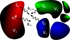
Figure 1: Schematic of a many-body geometry in which fluctuating current sources give rise to radiation as well as flux and momentum transfer between the bodies. Also illustrated are the incident field $\phi_{\mathrm{inc}}$ due to a single dipole source $\sigma$ within a body $V_{1}$ along with the induced polarization–currents $\xi$ throughout $V_{1}$ and two nearby bodies, $V_{2}$ and $V_{3}$, resulting in scattered fields $\phi_{\mathrm{scat}}$. The characteristics of the dipole sources $\sigma$ (fluctuation statistics) and the permittivities of the bodies $\chi$ (material properties) both vary within each object.

II.1 Volume integral equations

The derivations of VIEs often rely on the volume equivalence principle, which shares many similarities with—but is significantly simpler and more easily derived than—the more well-known surface equivalence principle Stratton and Chu (1939); Chen (1989); Harringston (1989). Consider the system of arbitrarily shaped, inhomogeneous bodies described by the relative permittivity $\epsilon$ and permeability $\mu$ functions, depicted schematically in Fig. 1. Let $\phi$ and $\sigma$ denote 6-component electromagnetic fields and volume currents,

$$\phi=\begin{pmatrix}\mathbf{E}\\ \mathbf{H}\end{pmatrix},\quad\sigma=\begin{pmatrix}\mathbf{J}\\ \mathbf{M}\end{pmatrix}.$$

and consider the scattering problem involving incident fields $\phi_{\rm inc}$ due to $\sigma$ (in the absence of bodies) and scattered fields $\phi_{\rm scat}$ due to reflections and scattering from objects and sources. Defining the 6-component volume currents

$$\xi=\begin{pmatrix}\mathbf{J}_{b}\\ \mathbf{M}_{b}\end{pmatrix}=-i\omega\chi\phi$$ (1)

associated with bound polarization $\mathbf{J}_{b}$ and magnetization $\mathbf{M}_{b}$ currents inside the objects, described by the $6\times 6$ susceptibility tensor $\chi$ (which for convenience also includes the permittivity and permeability of the ambient medium), it follows that the scattered field can be be written as a convolution of $\xi$ with the homogeneous Green’s function of the ambient medium Chew et al. (2001a). (Note that there is no assumption on $\chi$, which can describe both anisotropic and/or chiral media, changing only the form of the homogeneous Green’s function Staelin et al. (1994).) In particular, the unknown scattered fields can be shown to be related to the free and bound currents, respectively, via convolutions $(\star)$ with the $6\times 6$ homogeneous Green’s tensor of the ambient medium (typically free space) $\Gamma(\mathbf{x},\mathbf{y})=\Gamma(\mathbf{x}-\mathbf{y},\mathbf{0})$, written explicitly in Rodriguez et al. (2013). This is the core idea behind the volume equivalence principle, which we review below.

We begin by writing the total field $\phi=\Gamma\star(\sigma+\xi)$ via the volume equivalence principle Chew et al. (2001a) in terms of the incident $\phi_{\rm inc}=\Gamma\star\sigma$ and scattered $\phi_{\rm scat}=\Gamma\star\xi$ fields, or more explicitly:

$$\begin{split}\phi(\mathbf{x})&=\int d^{3}\mathbf{y}\,\Gamma(\mathbf{x},\mathbf{y})\left[\sigma(\mathbf{y})+\xi(\mathbf{y})\right]\end{split}$$ (2)

where it is clear that all of the scattering information (including material inhomogeneities) is “encoded” in the convolution of the homogeneous Green’s function with the polarization/magnetization current. Multiplying both sides of Eq. 2 with $-i\omega\chi$ and using the definition of $\xi$ in Eq. 1, one arrives at the following VIE for the induced currents $\xi$:

$$\xi+i\omega\chi(\Gamma\star\xi)=-i\omega\chi(\Gamma\star\sigma),$$ (3)

which can be solved to obtain $\xi$ from the incident sources $\sigma$. This is the so-called JM-VIE formulation of electromagnetic scattering in which the unknowns are induced currents rather than fields or field densities. Compared to other formulations based on field unknowns, JM-VIE exhibits superior performance in terms of accuracy and convergence, especially for objects with high refractive index Markkanen et al. (2012b); Polimeridis et al. (2014).

The operator equation above is customarily solved by reducing it to an approximate, finite-dimensional linear system. Let $\{b_{\alpha}\}$ be some convenient set of $N$ vector-valued basis functions. We can then approximate our unknowns $\xi$ (and, for convenience below, the source currents $\sigma$) in this basis:

$$\xi(\mathbf{x})\approx\sum\limits_{\alpha=1}^{N}x_{\alpha}b_{\alpha}(\mathbf{x}),\quad\sigma(\mathbf{x})\approx\sum\limits_{\alpha=1}^{N}s_{\alpha}b_{\alpha}(\mathbf{x}).$$ (4)

There are two main categories of basis functions that are used in the numerical solution of the JM-VIE above, known as spectral and MoM sub-domain bases. A spectral basis consists of non-localized Fourier-like basis functions whereas MoM sub-domain bases are localized functions obtained by discretizing objects into meshes or grids of volumetric elements, e.g. cubes, tetrahedra, and hexahedra Kolundzija and Djordjevic (2002), and defining functions by low-order polynomials with local support in one or a few elements. In this work, we resort to the second category and exploit piecewise constant basis functions defined in cubes, due to the flexibility they offer for modeling geometries of arbitrary shape Polimeridis et al. (2014). We note however that the proposed framework and the resulting matrix-trace formulas can also be evaluated using spectral bases as well.

Finally, the semi-discrete equation is “tested” with another set of functions (called testing functions) to produce a linear system. In the Galerkin approach, the set of testing functions is the same with the one of the basis functions. The resulting Galerkin JM-VIE linear system reads

$${W}^{-1}\,{x}=({V}-{W}^{-1})\,{s},$$ (5)

where

$$\begin{split}{W}^{-1}_{\alpha,\beta}&=\langle b_{\alpha},b_{\beta}+i\omega\chi(\Gamma\star b_{\beta})\rangle\\ {V}_{\alpha,\beta}&=\langle b_{\alpha},b_{\beta}\rangle\end{split}$$ (6)

and $\alpha,\beta=1:N$. Also, $\langle,\rangle$ denotes the standard inner product of functions $\langle\phi,\psi\rangle=\int\phi^{\ast}\psi$, with the $\ast$ superscripts denoting the conjugate transpose (adjoint) operation. Without loss of generality, we can choose the basis functions to satisfy an orthogonality relation, so that $\langle b_{\alpha},b_{\beta}\rangle=\delta_{\alpha\beta}$. In this case the matrix ${V}$ (often called Gram matrix) is equal to the identity matrix, i.e., ${V}\equiv{I}$, and it follows that

$${x}+{s}={W}{V}\,{s}={W}\,{s}.$$ (7)

Note that our simplifying assumption of orthogonal basis functions can be easily relaxed, leading to slightly modified $W\to WV$ and $C\to CV$ matrices (below).

The numerical evaluation of Galerkin inner products in Eq. 6 involves multidimensional integrals over the support of both basis and testing functions. This integration can be quite cumbersome due to singularities (when the support of the basis and the testing functions overlap) and the highly dimensional aspect of the problem. However, previous workPolimeridis et al. (2013a) demonstrated that these challenging volumetric integrals can be reduced to surface integrals (of lower singularity), allowing us to benefit from decades of work dedicated to the accurate and efficient evaluation of the associated surface integrals. Here, we make use of the free-software DEMCEMDEM (2011) and DIRECTFNDIR (2012), which leverage the techniques described in Refs. Polimeridis et al., 2013a, b . Furthermore, MoM JM-VIE formulations with local basis/testing functions typically result in very large linear systems, which can be solved with iterative algorithms for non-symmetric dense systems. In each iteration, the associated matrix-vector products take ${\cal{O}}(N^{2})$ time. Moreover, it is practically impossible to explicitly store the (dense) matrix ${W}^{-1}$ requiring ${\cal{O}}(N^{2})$ memory. In fact, there are now well-established, fast algorithms to reduce the costs of such integral equation solvers Philips and White (1997); Järvenpää et al. (2013); Polimeridis et al. (2014). However, the ability to exploit fast solvers in fluctuation EM problems is not a priori guaranteed since as we show below the final formulas involve complicated traces of products of JM-VIE and related matrices. In Sec. III, we describe a fast procedure for the computation of the proposed matrix-trace, which relies on a straightforward and easily implemented FFT-based fast algorithm presented in Polimeridis et al. (2014) that scales as ${\cal{O}}(N\log{N})$ for each matrix-vector product and requires ${\cal{O}}(N)$ memory.

Before concluding this section, we introduce some additional definitions and notation. In particular, further below we exploit the so-called Green matrix ${G}$, defined as

$${G}_{\alpha,\beta}=\langle b_{\alpha},\Gamma\star b_{\beta}\rangle,$$ (8)

which involves interactions among basis functions mediated by the Green’s function. For $n$ objects, the associated matrices and vectors can be conveniently written as:

$${G}\rightarrow\begin{pmatrix}{G}^{11}&{G}^{12}&\cdots&{G}^{1n}\\[5.0pt] {G}^{21}&{G}^{22}&\ldots&\vdots\\[5.0pt] \vdots&\vdots&\ddots&\vdots\\[5.0pt] {G}^{n1}&{G}^{n2}&\cdots&{G}^{nn}\end{pmatrix};\quad{\xi}\rightarrow\begin{pmatrix}{\xi}^{1}\\[5.0pt] {\xi}^{2}\\[5.0pt] \vdots\\[5.0pt] {\xi}^{n}\end{pmatrix}$$ (9)

where the superscripts denote blocks associated with the various objects, with diagonal components corresponding to self-interactions and off-diagonal blocks involving interactions between different objects. Finally, we define the projection,

$${P}^{p}_{\alpha,\beta}=\begin{cases}1,&\mbox{if }\alpha=\beta=p\\ 0,&\mbox{otherwise},\end{cases}$$ (10)

which selects specific blocks of vectors $\hat{x}^{p}=P^{p}x$ or diagonal blocks of matrices $\hat{A}^{p}=P^{p}AP^{p}$ corresponding to object $p$.

II.2 Power transfer

We now derive a compact matrix-trace formula for the computation of the ensemble-averaged flux into body ${\cal{B}}_{p}$ (or equivalently the absorbed power) due to fluctuating current sources in body ${\cal{B}}_{q}$, integrated over all possible positions and orientations. The first step consists of the evaluation of the flux from ${\cal{B}}_{p}$ due to a single dipole source $\sigma$ immersed in ${\cal{B}}_{q}$, which we denote as $\Phi^{q\rightarrow p}_{\sigma}$. Direct application of Poynting’s theorem implies that the flux on the objects is given by: Jackson (1999)

$$\Phi^{q\rightarrow p}_{\sigma}=\frac{1}{2}\operatorname{Re}{}\int_{{\cal{B}}_{p}}d^{3}\mathbf{x}\,\xi^{\ast}\cdot\phi$$ (11)

which amounts to the work done by the total field on the polarization currents in ${\cal{B}}_{q}$. Expressing the induced currents and fields in the basis of JM-VIE currents and using the relation $\phi=\Gamma\ast(\xi+\sigma)$ yields the following discrete approximation (see Polimeridis et al. (2015) for a complete analysis):

$$\begin{split}\Phi^{q\rightarrow p}_{\sigma}&=\frac{1}{2}\operatorname{Re}{}{x}^{p\ast}{\phi}^{p}=\frac{1}{2}\operatorname{Re}{}{x}^{\ast}{P}^{p}{\phi}\\ &=\frac{1}{2}\operatorname{Re}{}({x}+\hat{{s}}^{q})^{\ast}{P}^{p}{G}({x}+\hat{{s}}^{q})\\ &=\frac{1}{2}({x}+\hat{{s}}^{q})^{\ast}\operatorname{sym}{({P}^{p}{G})}({x}+\hat{{x}}^{q})\\ &=\frac{1}{2}\left({W}{P}^{q}{s}\right)^{\ast}\operatorname{sym}{({P}^{p}{G})}\left({W}{P}^{q}{s}\right)\\ &=\frac{1}{2}{\rm Tr}\left[({s}{s}^{\ast})({W}{P}^{q})^{\ast}\operatorname{sym}{({P}^{p}{G})}({W}{P}^{q})\right]\end{split}$$ (12)

where $\operatorname{sym}{{G}}=\frac{G+G^{*}}{2}$ denotes the Hermitian part of ${G}$. It is then straightforward to obtain the ensemble-averaged flux $\Phi^{q\rightarrow p}\equiv\langle\Phi^{q\rightarrow p}_{\sigma}\rangle$, which yields:

$$\begin{split}\Phi^{q\rightarrow p}&=\frac{1}{2}{\rm Tr}\left[\langle{s}{s}^{\ast}\rangle({W}{P}^{q})^{\ast}\operatorname{sym}{({P}^{p}{G})}({W}{P}^{q})\right]\\ &=\frac{1}{2}{\rm Tr}\left[{P}^{q}{C}{P}^{q}{W}^{\ast}\operatorname{sym}{({P}^{p}{G})}{W}\right]\end{split}$$ (13)

where ${C}=\langle{s}{s}^{\ast}\rangle$ is a current–current correlation matrix that captures a statistical, ensemble average over sources, described in more detail in Sec. II.5. Defining the matrix $\hat{C}^{q}=P^{q}CP^{q}$, which is simply a projection of the correlation matrix unto the space of basis functions in $q$, we find that the ensemble-averaged flux is given by:

$$\boxed{\Phi^{q\rightarrow p}=\frac{1}{2}{\rm Tr}\left[\hat{{C}}^{q}{W}^{\ast}\operatorname{sym}{({P}^{p}{G})}{W}\right].}$$ (14)

II.3 Momentum transfer

In addition to carrying energy, the radiation emitted by fluctuating sources also carries linear and angular momentum, which can also be described using similar expressions. The starting point consists of the evaluation of the force (or torque) imparted on an object ${\cal{B}}_{p}$ due to a single dipole source immersed in ${\cal{B}}_{q}$. Although electromagnetic forces are often computed via surface-integrals of the Maxwell stress tensor, it is also possible and in our case more convenient to express the force as a volume integral by considering the Lorentz force acting on the internal currents $\xi$ induced on ${\cal{B}}_{p}$ Krüger et al. (2012). In particular, the force on the object is given by:

$$\mathbf{F}^{q\to p}_{\sigma} =\frac{1}{2\omega}\text{Im }\int_{{\cal{B}}_{p}}d^{3}\mathbf{x}\,\xi^{*}\cdot\nabla\phi$$ (15)

where $\nabla$ denotes the usual partial derivative with respect to infinitesimal displacements. The derivation of the above expression follows from application of the time-average Lorentz force $d\mathbf{F}=\frac{1}{2}\text{Re }(\rho^{*}\mathbf{E}+\mathbf{J}^{*}\times\mathbf{B})d^{3}\mathbf{x}$ on the electric charge and current densities ($\rho,\mathbf{J}$) in an infinitesimal volume element $d^{3}\mathbf{x}$, together with a similar expression for the force on the magnetic sources. Integrating over the volume of the body and employing Stokes’ theorem along with Maxwell’s equations immediately yields Eq. 15. In a similar fashion, the torque about some origin $\mathbf{x}_{0}$ can be obtained by integrating the differential torque $d\boldsymbol{\tau}=(\mathbf{x}-\mathbf{x}_{0})\times d\mathbf{F}$ on a volume element.

Expressing the induced currents and fields in the basis of JM-VIE currents and following a similar procedure as that of Sec. II.2, one finds that the ensemble-averaged force on the object can be written in the compact and convenient form:

$$\boxed{\mathbf{F}^{q\to p}=\frac{1}{2\omega}\text{Tr }\Big{[}\hat{C}^{q}W^{*}\operatorname{asym}\left(P^{p}G^{\mathrm{F}}\right)W\Big{]},}$$ (16)

where in this case and in contrast to power transfer, the relevant quantity is the matrix representation $G^{\mathrm{F}}$ of the gradient of the Green’s function operator $G$, whose matrix elements $G^{\mathrm{F}}_{\alpha,\beta}=\langle b_{\alpha},\nabla\Gamma\star b_{\beta}\rangle$. Also, $\operatorname{asym}{{G}}=\frac{G-G^{*}}{2}$ denotes the skew-Hermitian part of ${G}$. The torque on the object can be obtained similarly by computing angular derivatives of $G$. It turns out that the calculation of these matrix elements requires evaluating multidimensional integrals whose singularities are more severe than those of $G$. A key distinction between fluctuation-induced transfers of power and momentum is that, in the latter case, one finds nonzero fluctuation-induced forces and torques between bodies even at thermal equilibrium and even at zero temperature; these are just the usual equilibrium Casimir forces. Reid et al. (2013) Equation 16, which computes only the non-equilibrium contribution to the force, must generally be augmented by these equilibrium contributions to yield the total force. Connections between Eq. 16 and expressions for equilibrium forces, along with techniques for evaluating the above-mentioned integrals and results of VIE computations of non-equilibrium Casimir forces and torques are addressed in subsequent work Reid et al. (2015).

II.4 Far-field radiation intensity

In addition to power and momentum transfer, another useful quantity is the far-field radiation intensity of our system, which can also be expressed as a simple trace formula. The result which follows trivially from Eq. 13, is that the ensemble-averaged flux radiated by an isolated body ${\cal{B}}_{q}$ to the background medium is given by:

$$\Phi^{q\rightarrow 0}=-\frac{1}{2}{\rm Tr}\left[{C}{W}^{\ast}\operatorname{sym}{{G}}{W}\right]$$ (17)

where the minus sign corresponds to the direction of the power flux and stems from Poynting’s theorem. However, in addition to the overall radiation, it is also useful to obtain the radiation intensity over specific directions, or equivalently the power radiated per solid angle. The angle-resolved radiation intensity $U_{\sigma}^{q\rightarrow 0}$ from a single source $\sigma$ immersed in ${\cal{B}}_{q}$ can be obtained by expressing the radiation field at infinity $\mathbf{E}_{\infty}$ (where only far field contributions remain) in terms of the free and bound current sources, as follows:

$$U^{q\rightarrow 0}_{\sigma}=\frac{k^{2}Z}{2(4\pi)^{2}}|Q\mathbf{e}_{\infty}(\mathbf{x})|^{2}=\frac{k^{2}Z}{2(4\pi)^{2}}|Q\left[\Gamma_{\infty}^{\rm E}\star(\sigma+\xi)\right]|^{2}$$ (18)

where $k$ is the wavenumber and $Z=\sqrt{\mu_{0}/\epsilon_{0}}$ is the wave impedance, both in vacuum. Also, $\Gamma_{\infty}^{\rm E}(\mathbf{x},\mathbf{y})$ is the $3\times 6$ Green’s tensor of the ambient medium which maps currents to far-field electric fields, and $Q$ is a $3\times 3$ transformation tensor that maps vectors from Cartesian to spherical coordinates and projects their radial component to zero Balanis (1997). Given the solution of the VIE scattering problem and following the same procedure described above, it is straightforward to write the radiation intensity as a matrix-trace formula of the form:

$$\begin{split}U^{q\rightarrow 0}_{\sigma}&=\frac{k^{2}Z}{2(4\pi)^{2}}({s}+{x})^{\ast}{G}_{\infty}^{\rm E\ast}{G}_{\infty}^{\rm E}({s}+{x})\\ &=\frac{k^{2}Z}{2(4\pi)^{2}}{\rm Tr}\left[({s}{s}^{\ast})({W})^{\ast}({G}_{\infty}^{\rm E\ast}{G}_{\infty}^{\rm E})({W})\right]\end{split}$$ (19)

where the matrix ${G}_{\infty}^{\rm E}$ is the discretized form of the operator $Q\Gamma_{\infty}^{\rm E}$, obtained in a similar fashion as ${G}$. Ensemble averaging over all sources, we find that the final formula for the angle-resolved radiation intensity $U^{q\rightarrow 0}\equiv\langle U^{q\rightarrow 0}_{\sigma}\rangle$ is given by:

$$\boxed{U^{q\rightarrow 0}=\frac{k^{2}Z}{2(4\pi)^{2}}{\rm Tr}\left[{C}\,{W}^{\ast}({G}_{\infty}^{\rm E\ast}{G}_{\infty}^{\rm E}){W}\right].}$$ (20)

Equation 20 can be integrated over all solid angles $\Omega$ to yield the total radiation rate $\Phi^{q\rightarrow 0}=\int d\Omega\,U^{q\rightarrow 0}(\Omega)$, which as expected agrees with results obtained by direct application of Eq. 17, as discussed in Sec. III.

II.5 Current–current correlation matrices

The formulas above are very general in that they apply to many different kinds of fluctuation processes, the physical properties and origins of which are embedded in the correlation matrices $C=\langle ss^{*}\rangle$, involving ensemble averages over all sources $\sigma$ and polarizations throughout the bodies. In particular, the matrix elements of the correlation matrices describe interactions among basis functions and are given by:

$$\begin{split}{C}_{\alpha,\beta}=\langle s_{\alpha}s_{\beta}^{\ast}\rangle=\int\int d^{3}\mathbf{x}d^{3}\mathbf{y}\,b_{\alpha}^{\ast}(\mathbf{x})\langle\sigma(\mathbf{x})\sigma^{\ast}(\mathbf{y})\rangle b_{\beta}(\mathbf{y})\end{split}$$ (21)

which follows trivially from the orthogonality property of our basis functions and the fact that $\sigma(\mathbf{x})=\sum_{\alpha}s_{\alpha}b_{\alpha}(\mathbf{x})$. Although in general the calculation of each matrix element involves volume–volume integrals against pairs of basis functions, current fluctuations are temporally and spatially uncorrelated in local media Agarwal (1974); Eckhardt (1984); Matloob et al. (1997) and are described by:

$$\langle\sigma_{i}(\mathbf{x},\omega)\sigma_{j}^{\ast}(\mathbf{y},\omega)\rangle=\mathcal{J}_{ij}(\mathbf{x},\omega)\delta(\mathbf{x}-\mathbf{y})$$ (22)

where the subscripts denote polarization degrees of freedom and $\mathcal{J}\geq 0$ is a position-dependent spectral tensor whose form depends on the physical origins of the fluctuations. It follows that $C$ is Hermitian and positive-semidefinite and thus admits a Cholesky factorization ${C}={L}_{{C}}{L}_{{C}}^{\ast}$, which we exploit in Sec. III to demonstrate that our radiation, power, and momentum formulas are susceptible to fast-trace calculations.

When the sources of fluctuations involve only quantum and thermal vibrations (heat), the correlation function $\mathcal{J}$ is determined by thermodynamic considerations such as the well-known FDT Lifshitz and Pitaevskii (1980); Eckhardt (1984), relating current fluctuations to dissipation in materials. Without loss of generality, the spectral function is given by: Lifshitz and Pitaevskii (1980)

$$\mathcal{J}_{ij}(\mathbf{x},\omega)=\frac{4}{\pi}\operatorname{Im}\chi_{ij}(\mathbf{x},\omega)\Theta(\mathbf{x},\omega),$$ (23)

where the $\operatorname{Im}\chi$ tensor describes losses in the medium and $\Theta(\mathbf{x},\omega)=\hbar\omega/(e^{\hbar\omega/k_{\rm B}T(\mathbf{x})}-1)$ is the Planck distribution, or the average energy of an oscillator having local temperature $T(\mathbf{x})$. Equation 23 in conjunction with the power transfer and radiation formulas above are exploited below to evaluate thermal radiation and heat transfer between inhomogeneous bodies with spatially varying temperature and dielectric properties, and also in an upcoming paper that focuses on non-equilibrium Casimir forces Reid et al. (2015).

In situations involving active media driven by external pumps, the properties of the fluctuating currents and hence $\mathcal{J}$ depend on the details of the input drive along with the physical emission mechanisms. For a broad range of processes, the spectral function can be written in the simple form:

$$\mathcal{J}_{ij}(\mathbf{x},\omega)=\chi_{\rm inc}(\mathbf{x})\chi_{\rm emm,ij}(\mathbf{x},\omega),$$ (24)

where $\chi_{\rm inc}$ describes the response of the medium due to the pump and $\chi_{\rm emm}$ describes the emission spectrum of the excited medium, which depends on the distribution of active molecules in the medium and on complicated electronic transitions mediated by the pump as well as quantum/thermal processes Le Ru and Etchegoin (2008). In the particular example of one-photon fluorescence from a medium (with high quantum yield) excited by incident light, the pump spectrum is proportional to the locally absorbed power and hence can be computed by direct application of the VIE power formulas. Such a relationship in conjunction with Eq. 20 is exploited below to compute the fluorescence spectrum of an irradiated sphere. A similar dependence on the local field intensity arises in the case of Raman scattering, except that $\chi_{\rm inc}$ is proportional to the Raman polarizability tensor rather than the susceptibility of the medium Le Ru and Etchegoin (2008). In the case of spontaneous emission from a gain medium, the emission spectrum is determined by spatially dependent effective permittivity and temperature profiles determined by the driven steady-state atomic populations of the medium, both of which can be obtained by application of steady-state ab-initio laser theory (SALT) Henry (1986); Matloob et al. (1997). Similar descriptions apply in more complicated systems, including fluorophores with low quantum yields or active media subject to highly nonlinear (e.g. two-photon) processes.

III Fast Trace Computations

The matrix-trace formulas derived in the previous sections require products of inverses of the JM-VIE matrix ${W}$ with dense matrices $\operatorname{sym}{({P}^{p}{G})}$, $\operatorname{asym}{({P}^{p}\nabla{G})}$, and ${G}_{\infty}^{\rm E\ast}{G}_{\infty}^{\rm E}$. As mentioned above, due to their large size and correspondingly severe CPU and memory limitations, it is practically impossible to form explicitly either the Green matrix or its inverse. There are however fast FFT-based procedures for evaluating matrix-vector products of the JM-VIE system matrix and the Green matrix Polimeridis et al. (2014). Here we describe a framework based on iterative methods for the fast computation of the associated trace formulas above.

We begin with the matrix-trace formula $\Phi^{q\rightarrow p}$ in the presence of $n$ bodies (including ${\cal{B}}_{p}$ and ${\cal{B}}_{q}$), which after some algebraic manipulations can be written as follows (ignoring pre-factors):

$$\begin{split}\Phi^{q\rightarrow p}&={\rm Tr}\left[{C}^{qq}{W}^{pq\ast}(\operatorname{sym}{{G}^{pp}}){W}^{pq}\right]\\ &+\sum\limits_{\begin{subarray}{c}m=1\\ m\neq p\end{subarray}}^{n}{\rm Tr}\left[{C}^{qq}\operatorname{sym}{\left({W}^{pq\ast}{G}^{pm}{W}^{mq}\right)}\right]\\ &=S^{q\rightarrow p}+C^{q\rightarrow p}\end{split}$$ (25)

where ${C}^{qq}$ is the $qq$ block of the matrix ${C}$. Due to the different characteristics of $S^{q\rightarrow p}$ and $C^{q\rightarrow p}$, we need to address them separately. As discussed in Sec. II.5, the matrix ${C}^{qq}$ can be assumed to be Hermitian and positive semidefinite, hence it admits a Cholesky factorization, ${C}^{qq}={L}_{{C}^{qq}}{L}_{{C}^{qq}}^{\ast}$. In addition, $\operatorname{sym}{{G}^{pp}}$ is a Hermitian, negative semidefinite matrixRodriguez et al. (2013) and it also admits a low-rank approximation since it is associated with the smooth, imaginary part of the Green’s functions. Hence, it can be approximated to any desired accuracy by a truncated singular value decomposition (SVD) factorization, $\operatorname{sym}{{G}^{pp}}\approx-{U^{pp}}{S^{pp}}{U^{pp}}^{\ast}$, where ${S^{pp}}\in\mathbb{C}^{r\times r}$, with $r\ll N$. The norm of the error in the aforementioned truncation is bounded by the norm of the vector of discarded singular values. The classical SVD algorithm requires the complete matrix, hence we resort here to a class of modern randomized matrix approximation techniques, and more specifically to the randomized SVD method (rSVD) Halko et al. (2011); Hochman et al. (2014). rSVD is effective for matrices with fast drop of the singular values and it requires only a fast matrix-vector procedure, which we have developed as described above. The matrix with the singular values can be further decomposed so that ${S^{pp}}={L_{S^{pp}}}{L_{S^{pp}}^{\ast}}$. Finally, it follows that the self-term in Eq. 25 can be written as the square of a Frobenius norm,

$$\begin{split}S^{q\rightarrow p}&=-{\rm Tr}\left[{L}_{{C}^{qq}}{L}_{{C}^{qq}}^{\ast}({W}^{pq\ast}{U^{pp}}){L_{S^{pp}}}{L_{S^{pp}}^{\ast}}({U^{pp\ast}}{W}^{pq})\right]\\ &=-\|{L}_{{C}^{qq}}^{\ast}({W}^{pq\ast}{U^{pp}}){L_{S^{pp}}}\|_{\rm F}^{2}.\end{split}$$ (26)

For the most time consuming part of the norm, we need to solve the adjoint JM-VIE system $r$ times (for each of the leading singular vectors of $\operatorname{sym}{{G}^{pp}}$). Note however that we can solve for each vector of ${U^{pp}}$ independently and thus the entire procedure is embarrassingly parallelizable. Also, ${L}_{{C}^{qq}}^{\ast}$ and ${L_{S^{pp}}}$ are either sparse or diagonal, while ${W}^{pq\ast}{U^{pp}}$ is a “tall-and-skinny” matrix (the number of columns is much smaller than the number of rows) and hence the matrix product appearing in the norm can be computed efficiently.

The trace formula for $C^{q\rightarrow p}$ is not symmetrical and therefore cannot be reduced to a norm. In this case, one can exploit the fact that ${G}^{pm}$ admits a low-rank approximation due to the smoothing properties of the Green’s function for disjoint objects. The final dimensions of the low-rank approximation of $C^{q\rightarrow p}$ (for a prescribed accuracy) depend on the electric distance between objects $p$ and $m$ Chai and Jiao (2003), i.e., ${G}^{pm}\approx{U^{pm}}{S^{pm}}{V^{pm}}^{\ast}$, where ${S^{pm}}\in\mathbb{C}^{l\times l}$, with $l\ll N$. The final formula for $C^{q\rightarrow p}$ after the Cholesky factorization of the singular values matrix (${S^{pm}}$) is given by

$$\begin{split}C^{q\rightarrow p}=\operatorname{Re}{}\sum\limits_{\begin{subarray}{c}m=1\\ m\neq p\end{subarray}}^{n}{\rm Tr}\left[{X_{U^{pm}}}{X_{V^{pm}}^{\ast}}\right]\end{split}$$ (27)

where

$$\begin{split}{X_{U^{pm}}}&={L}_{{C}^{qq}}^{\ast}({W}^{pq\ast}{U^{pm}}){L}_{{S^{pm}}}\\ {X_{V^{pm}}}&={L}_{{C}^{qq}}^{\ast}({W}^{mq\ast}{V^{pm}}){L}_{{S^{pm}}}.\end{split}$$

Both ${X_{U^{pm}}}$ and ${X_{V^{pm}}}$ are “tall-and-skinny”, and we can not compute the trace by forming explicitly their product, due to memory limitations. Alternatively, we can use the standard vectorization of a matrix ${\rm vec}()$, which converts the matrix into a column vector, together with the identity, ${\rm Tr}\left[{X}{Y}^{\ast}\right]={\rm vec}({X})^{T}\cdot\overline{{\rm vec}({Y})}$, and write Eq. 27 in the following computationally friendly form:

$$\begin{split}C^{q\rightarrow p}=\operatorname{Re}{}\sum\limits_{\begin{subarray}{c}m=1\\ m\neq p\end{subarray}}^{n}{\rm vec}({X_{U^{pm}}})^{T}\cdot\overline{{\rm vec}({X_{V^{pm}}})}.\end{split}$$ (28)

The overall computational complexity for the evaluation of $C^{q\rightarrow p}$ consists of a single run of the Randomized-SVD for a non-symmetric matrixHalko et al. (2011), and $2\times l$ solves of the adjoint JM-VIE system. In the case of the matrix-trace formulas for the force and the torque, the procedure is similar with the one described above. The only difference stems from the replacement of ${G}$ with $G^{\mathrm{F}}$ and $\operatorname{sym}{}$ with $\operatorname{asym}{}$.

Finally, the case of far-field radiation is somewhat simpler. According to Eq. 20, we just need to solve $2$ times the adjoint JM-VIE system, since ${G}_{\infty}^{\rm E\ast}\in\mathbb{C}^{N\times 2}$. Hence, the radiation intensity for a specific direction or solid angle $\Omega$, is given by the following square of the Frobenius norm:

$$\begin{split}U^{q\rightarrow p}(\Omega)=\frac{k^{2}Z}{2(4\pi)^{2}}\|{L}_{{C}}^{\ast}({W}^{\ast}{G}_{\infty}^{\rm E\ast})\|_{\rm F}^{2}.\end{split}$$ (29)

This is a very useful formula, especially when directional information of the radiated power is of interest. In addition, the total radiated power can be evaluated by integrating Eq. 29 over all solid angles, as mentioned in Sec. II.4, which would amount to employing a numerical integration scheme over the unit sphere (e.g. Lebedev quadrature Lebedev (1976)). Alternatively, one could exploit Eq. 17 and the associated norm $\|{L}_{{C}}^{\ast}({W}^{\ast}{U}){L_{S}}\|_{\rm F}^{2}$ to compute the total radiated power from an isolated body. The latter is expected to be more efficient for total-radiation computations with prescribed accuracy, controlled by the SVD factorization of the Green matrix, in which case the minimum number of JM-VIE solves needed for a prescribed accuracy is estimated in advance. In contrast, the former approach is based on adaptive quadrature schemes where the accuracy is controlled by the comparison of results between different orders of integration, with no a priori control.

IV Validation and Applications

In this section, we apply the FVC method to obtain new results in complex geometries. To begin with, we show that the Green matrices appearing in our trace formulas admit low-rank decompositions (as discussed in Sec. III) by computing their ranks to within some tolerance in a representative structure involving two vacuum-separated, homogeneous cubes. We validate the FVC method by checking its predictions against known results of thermal radiation and near-field heat transfer between homogeneous bodies, including spheres, cubes, and ellipsoids, obtained using a boundary-element implementation of our recent FSC formulation Rodriguez et al. (2013). We show that when subject to temperature gradients or continuously varying permittivities, complex bodies can exhibit highly modified thermal radiation and heat transfer spectra, leading to directional emission at selective wavelengths. Finally, we demonstrate that the same formalism can be exploited to study luminescence from excited media by computing the fluorescence spectrum of a sphere irradiated by monochromatic incident light. We show that the impact of the resulting inhomogeneous current fluctuations cannot be easily obtained by exploiting simple homogenization or effective-medium approximations. For convenience and simplicity, we consider dielectric media with no material dispersion (constant $\operatorname{Re}\epsilon\approx 12$ and large dissipation $\operatorname{Im}\epsilon\approx 1$), though our approach is general in that it can readily handle other kinds of materials such as metals with $\operatorname{Re}\epsilon<0$ and even gain media.

IV.1 Low-rank approximations

Low-rank approximations of the associated (free-space) Green matrices are instrumental to the practical and efficient evaluation of our trace formulas. In this section, we present some representative results obtained from computing the ranks of both $\operatorname{sym}{{G}^{pp}}$ and ${G}^{pm}$, to within some tolerance, for the particular problem of two vacuum-separated, homogeneous cubes of edge-length $L=2R$ and separated by a surface–surface distance $d$, shown schematically in Fig. 5.

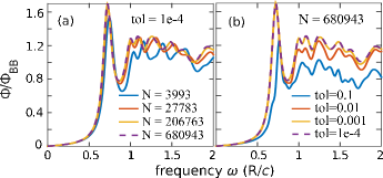
Figure 2: Flux spectrum $\Phi(\omega)$ of a cube of edge-length $2R$ held at temperature $T$, normalized by the corresponding black-body spectrum $\Phi_{\mathrm{BB}}(\omega)=\frac{A}{4\pi^{2}}(\omega/c)^{2}\Theta(\omega,T)$, for different (a) discretization mesh densities and (b) rSVD truncation tolerances.

Table 1: Ranks of $\operatorname{sym}{{G}^{11}}$ for various frequencies ($\omega\frac{R}{c}$) and tolerances (tol) in truncated SVD. The ranks correspond to the case of a cube of edge-length $2R$. In addition, results for a sphere of radius $R$ are included in brackets.

	$1e^{-1}$	$1e^{-2}$	$1e^{-3}$	$1e^{-4}$	$1e^{-5}$	$1e^{-6}$
0.01	4 (4)	4 (4)	4 (4)	4 (4)	7 (7)	12 (12)
0.1	4 (4)	4 (4)	7 (7)	12 (12)	12 (12)	14 (12)
1.0	12 (7)	14 (12)	24 (24)	40 (24)	40 (40)	60 (40)
2.0	18 (12)	37 (24)	51 (40)	65 (60)	84 (60)	109 (84)

Table 2: Ranks of ${G}^{12}$ for various distances ($d$) and tolerances (tol) in truncated SVD. The ranks correspond to the case of two cubes of edge length $L=2R$ and frequency $\omega\frac{R}{c}=1$. Each cube is discretized into $N=40^{3}$ voxels, resulting in $3N$ total degrees of freedom, i.e., $\#\rm{DOFS}=3N$.

	$1e^{-1}$	$1e^{-2}$	$1e^{-3}$	$1e^{-4}$	$1e^{-5}$	$1e^{-6}$
0.001	4075	4853	5253	6352	7240	8481
0.01	992	2611	3934	4800	5832	6894
0.1	50	196	447	804	1268	1849
1.0	6	14	27	42	66	89
10.0	4	7	9	14	19	23

Table I shows the singular values of $\operatorname{sym}{{G}^{11}}$, corresponding to one of the two cubes, as a function of the normalized frequency $\omega R/c$ and tolerance $\rm tol$; that is, we obtain the singular values that produce SVD factorizations bounded in norm by the tolerance $\rm tol$, also known as a truncated SVD. Since the associated matrix is very large and our trace formulations can be cast in terms of fast matrix–vector products, our calculations exploit the rSVD method recently developed for big-data problems Halko et al. (2011). (Note that results for the second cube, involving $\operatorname{sym}{{G}^{22}}$, would be identical since both cubes have equal sizes and number of unknowns.) Our results reveal at least two important features: First, the ranks scale linearly with $\omega$ at large frequencies, and sub-linearly (roughly constant) at small frequencies. Additional numerical experiments (not shown) confirm that the effect of mesh density on the ranks is negligible, yet another manifestation of the favourable convergence properties of the JM-VIE formulation Polimeridis et al. (2014). This also suggests a strategy for obtaining the finite rank of $\operatorname{sym}{{G}^{pp}}$ with prescribed accuracy: we begin by computing the rank of the operator for a prescribed accuracy by using a coarse mesh and then run a fixed-rank rSVD algorithm with finer mesh. Finally, Fig. 2 illustrates the rate of convergence of the radiation spectrum $\Phi(\omega)$ from an isolated cube at a fixed temperature $T$ with respect to different (a) discretization mesh densities and (b) truncation tolerance, normalized to the spectrum of a corresponding black body $\Phi_{\mathrm{BB}}(\omega)=\frac{A}{4\pi^{2}}(\omega/c)^{2}\Theta(\omega,T)$, where $A$ denotes the surface area of the cube.

The situation changes in the case of the “coupling” Green matrix ${G}^{12}$, which encodes interactions between objects. Table II shows the significant singular values associated with the coupling matrix of the same cube–cube geometry at a fixed frequency $\omega$ and for various separations $d$, obtained by leveraging the rSVD technique. As expected, the singular values increase as $d$ decreases, a consequence of the power-law drop-off of the Green’s function with separation in the near field. It follows that the computation complexity of the trace formulas increases as the two bodies come close together. (Note that, as described in Sec. III, our trace formulas for power and momentum transfer require us to solve two VIE systems for every corresponding eigenvector, but fortunately each system can be solved independently and the overall process is embarrassingly parallelizable.) Nevertheless, we find that $G^{12}$ remains very low rank even for relatively close separations $d/L\approx 0.1$, below which constraints on the resolution make the FVC approach less practical. However, it is precisely at such small separations that approximate methods such as the proximity approximation become accurate Sasihithlu and Narayanaswamy (2013).

IV.2 Thermal radiation and heat transfer

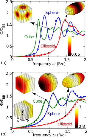
Figure 3: Flux spectrum $\Phi(\omega)$ normalized by the corresponding black-body spectrum $\Phi_{\mathrm{BB}}(\omega)=\frac{A}{4\pi^{2}}(\omega/c)^{2}\Theta(\omega,T)$ of different bodies of surface area $A$ held at temperature $T=1000$ K, including a sphere of radius $R$ (blue lines), cube of edge-length $2R$ (green line), and ellipsoid of long semi-axis $R$ and short semi-axis $\frac{R}{2}$ (red line). The objects have either (a) uniform permittivities $\epsilon=12+i$ or (b) spatially varying $\epsilon(z)=\epsilon_{-R}+(\epsilon_{R}-\epsilon_{-R})\frac{|z+R|}{2R}$, with $\epsilon_{R}=12+i$ and $\epsilon_{-R}=2+i$. For comparison, we also plot the radiation spectrum $\Phi_{\rm eff}$ (dashed lines) of corresponding bodies with homogeneous effective permittivities $\epsilon_{\rm eff}=7+i$. The insets depict the angular distribution of far-field radiation $U(\Omega)$, normalized by the maximum intensity over all directions $\max_{\Omega}U$, at selected frequencies.

We begin by validating our FVC approach by checking its predictions of thermal radiation from homogeneous bodies against results obtained using our recently developed FSC formulation Rodriguez et al. (2013); Rodriguez et. al. (2013), which is well-suited for handling piece-wise constant structures and fluctuations statistics. Figure 3(a) shows the flux spectra $\Phi(\omega)$ of multiple objects (of uniform temperature $T$ and permittivity $\epsilon=12+i$, including a sphere of radius $R$ (blue line), a cube of edge-length $2R$ (green line), and an prolate ellipsoid of long semi-axis $R$ and short semi-axes $\frac{R}{2}$ (red line). Note that in each case $\Phi(\omega)$ is normalized to the corresponding flux from a black body. As shown, there is excellent agreement between the FVC (solid lines) and FSC (circles) predictions, both of which illustrate the expected radiation enhancement at geometric resonances.

The FVC method can also handle more complex structures, including inhomogeneous bodies with spatially varying permittivities. In particular, Fig. 3(b) shows $\Phi(\omega)$ for the same geometries of Fig. 3(a) but for objects with linearly varying permittivity profiles $\epsilon(z)=\epsilon_{-R}+(\epsilon_{R}-\epsilon_{-R})\frac{|z+R|}{2R}$, with $\epsilon_{-R}=2+i$ and $\epsilon_{R}=12+i$ (solid lines) and axes chosen to lie at the geometric center of each object. Compared to the spectrum of the homogeneous bodies of Fig. 3(a), one finds that the resonances are shifted to larger frequencies and their peak amplitudes are significantly smaller, a consequence of the decreased effective permittivity of each object. For comparison, we also show $\Phi_{\rm eff}(\omega)$ (dashed lines) from corresponding homogeneous objects with effective permittivities,

$$\epsilon_{\rm eff}=\frac{1}{V}\int_{V}d^{3}\mathbf{x}\,\epsilon(\mathbf{x}),$$ (30)

corresponding to uniform $\epsilon_{\rm eff}=7+i$. Our calculations reveal that in the illustrated frequency range and for our choice of dielectric profiles, the homogeneous approximation is qualitatively accurate to within $10\%$. On the other hand, employing Eq. 20 to compute the angular radiation patterns at selected frequencies, shown as insets in Fig. 3, reveals significant changes, e.g. significantly larger directional emission, that cannot be captured by the effective-medium approximation. In particular, the radiation patterns of the inhomogeneous objects break $\hat{z}$ mirror symmetry. For example, the flux from the cube at $\omega\approx 0.65R/c$ is slightly larger in the $-\hat{z}$ than in the $+\hat{z}$ direction, a situation that is reversed at larger $\omega\approx 0.9R/c$ (see insets). Generally, the transition frequency of the favored radiation direction depends on the geometry; for instance, even at a frequency as high as $\omega\approx 1.5R/c$, the ellipsoid continues to radiate more along the $-\hat{z}$ direction.

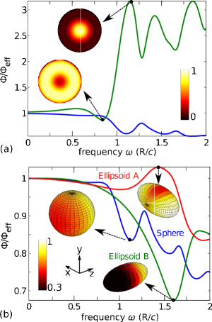
Figure 4: Flux spectrum $\Phi(\omega)$ of various bodies normalized by the corresponding predictions of a simple approximation $\Phi_{\mathrm{eff}}$, defined in Eq. 31, including (a) sphere of radius $R$ and radially varying temperature profile $T(r)=T_{0}+(T_{R}-T_{0})\frac{r}{R}$ for both $T_{0}=0,T_{R}=1000$ K (blue line) and $T_{0}=1000,T_{R}=0$ (green line), and (b) sphere of radius $R$ (blue line) or ellipsoids with short semi-axes $\frac{R}{2}$ and long semi-axis $R$ along the $\hat{z}$ (green line) or $\hat{x}$ (red line) directions, subject to vertically varying temperature profiles $T(z)=T_{-L}+(T_{L}-T_{-L})\frac{|z+L/2|}{L}$, where $L$ denotes the $z$-dimension of the corresponding body. In all cases, objects have uniform permittivity $\epsilon=12+i$ and are subject to temperature gradients $T_{-L}=0$ and $T_{L}=1000$ K. The insets in (a) show the local density of states along a cross-section of the sphere at different frequencies while those in (b) show the angular distribution of far-field radiation $U(\Omega)$ normalized by $\max_{\Omega}U$.

More pronounced changes arise when objects are subject to spatial temperature gradients. Figure 4 shows $\Phi(\omega)$ from homogeneous ($\epsilon=12+i$) ellipsoids subject to either (a) radially varying $T(r)=T_{0}+(T_{R}-T_{0})\frac{r}{R}$ or (b) $z$-varying temperature profiles (see caption). In both cases, $\Phi$ is normalized by the flux $\Phi_{\mathrm{eff}}$ obtained from a naive approximation in which the temperature variations are removed in favor of a uniform effective temperature $T_{\mathrm{eff}}$ determined by a simple average of the Planck distribution over the volume $V$ of the bodies,

$$\Theta(\omega,T_{\mathrm{eff}})=\frac{1}{V}\int_{V}d^{3}\mathbf{x}\,\Theta(\omega,T(\mathbf{x})).$$ (31)

Such a simple approximation obviates the need for exact calculations that explicitly incorporate inhomogeneities, but is clearly inadequate for wavelength-scale objects. Specifically, Fig. 4(a) shows $\Phi(\omega)$ from spheres with radially varying temperatures, illustrating that beyond the sub-wavelength regime $\omega\ll R/c$ and depending on the choice of $T_{0}$ and $T_{R}$, $\Phi$ can be many times larger or smaller than that predicted by Eq. 31. The failure of this naive approximation is especially apparent near resonances, where the coupling of fluctuating sources (dipoles) to far-field radiation (the local density of states) is highly position-dependent. The insets of Fig. 4(a) show cross-sections of the spatially varying flux contribution from dipoles in the interior of the sphere at two relatively close frequencies. At $\omega R/c\approx 1.1$, we find that dipoles closer to the center can couple more efficiently to far-field radiation than those near the edges, causing Eq. 31 to underestimate the flux by $\Phi/\Phi_{\mathrm{eff}}\approx 3$ in the case $T_{0}=0$, $T_{R}=1000$ K (green line) and to overestimate it by $\Phi/\Phi_{\mathrm{eff}}\approx 0.8$ when $T_{0}=1000\leavevmode\nobreak\ \mathrm{K}$, $T_{R}=0$ (blue line). The converse is true at $\omega R/c\approx 0.85$, in which case their coupling to radiation is largest at the center and edges of the sphere. Similar effects arise in situations involving $z$-varying temperature profiles, explored in Fig. 4(b) for either spheres (blue line) or ellipsoids with either their long-axes (green line) or short-axes (red line) aligned with the $\hat{z}$ direction. For instance, ellipsoids can exhibit highly directional emission (almost a factor of 3 times larger) along the direction of increasing temperature.

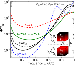
Figure 5: Heat-transfer spectrum $\Phi(\omega)$, normalized by the corresponding black-body spectrum $\Phi_{\mathrm{BB}}(\omega)=\frac{A}{4\pi^{2}}(\omega/c)^{2}\Theta(\omega,T)$, between two cubes of edge-length $2R$ and temperature $T=1000$ K separated by surface–surface distance $d=R$. The cubes are assumed to have either uniform permittivities $\epsilon=2+i$ (red dashed line), $\epsilon=\epsilon_{\mathrm{eff}}=7+i$ (black dashed line), or $\epsilon=12+i$ (blue dashed line), or vertically varying permittivities $\epsilon(z_{i})=\epsilon_{-R}+(\epsilon_{R}-\epsilon_{-R})\frac{|z_{i}+R|}{2R}$ defined with respect to the local axis $\mathbf{x}_{1,2}$ at the center of each cube (shown on the inset), chosen so that the system has mirror symmetry about the $x$–$y$ plane intersecting the origin $O$. The gradients are either increasing (black solid line) or decreasing (green solid line) toward or away from the center, corresponding to the choice of $\epsilon_{R,-R}=\{12+i,2+i\}$ or $\epsilon_{R}\leftrightarrow\epsilon_{-R}$, respectively.

In addition to far-field radiation, the FVC method can be employed to obtain radiative transfer between objects. Figure 5 shows the heat-transfer spectrum $\Phi(\omega)$ (computed via Eq. 16) normalized by $\Phi_{\mathrm{BB}}(\omega)$ (same as above), between two vacuum-separated cubes of edge-length $2R$ and surface–surface separation $d=R$, of either uniform (dashed lines) or vertically varying (solid lines) permittivities. We consider dielectric profiles of the form $\epsilon(z_{i})=\epsilon_{-R}+(\epsilon_{R}-\epsilon_{-R})\frac{|z_{i}+R|}{2R}$ defined with respect to the local axis located at the center of each cube $\mathbf{x}_{1,2}$, chosen so that the entire system has mirror symmetry about the origin (see inset). We consider two different profiles, $\epsilon_{-R,R}=\{2+i,12+i\}$ (black line) or $\epsilon_{R}\leftrightarrow\epsilon_{-R}$ (green line), corresponding to increasing gradients toward or away from the origin. For comparison, we also plot the transfer between cubes of uniform permittivities $\epsilon=2+i$ (red dashed line), $\epsilon=12+i$ (green dashed line), and $\epsilon=\epsilon_{\rm eff}=\frac{1}{V}\int_{V}d^{3}\mathbf{x}\,\epsilon(z)$, corresponding to the minimum, maximum, or average of the spatially varying permittivities, respectively. As shown, depending on the wavelength regime (near versus far field) inhomogeneities can have a different effect on the heat transer. For instance, at low $\omega R/c\ll 1$ where near-field effects prevail, homogeneous bodies with smaller dielectric constants tend to transfer more heat—the same dependence is observed for planar objects separated by vacuum, where the near-field contribution $\sim(\frac{\operatorname{Im}\epsilon}{|\epsilon+1|^{2}})^{2}$ Basu et al. (2009). Not surprisingly, because nearby regions tend to contribute more than far-away regions, one observes that despite having the same average permittivities $\epsilon_{\rm eff}$ (dashed blue line), the transfer is sensitive to the local dielectric variation, exhibiting larger enhancement in the case where the permittivity is increasing toward (green solid line) rather than away (black solid line) from the origin. At larger $\omega R/c\gtrsim 0.5$ where far-field effects begin to dominate, one observes the opposite behavior, in which case the largest transfer is obtained for decreasing permittivities toward the origin. Essentially, as illustrated in Fig. 3(b), at sufficiently large wavelengths, bodies with dielectric gradients tend to radiate along the direction of increasing permittivity.

IV.3 Fluorescence

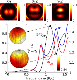
Figure 6: Far-field fluorescence spectrum $\Phi(\omega)$ (in arbitrary units) of a homogeneous and non-dispersive dielectric sphere of radius $R$ and permittivity $\epsilon=12+i$ excited by an $\hat{x}$-polarized planewave propagating along the $\hat{z}$ direction with frequency $\omega_{\mathrm{inc}}R/c=1.58$. The absorbed power $\chi_{\rm inc}(\mathbf{x})$ inside the sphere, obtained by solving a single scattering problem as described in Polimeridis et al. (2014), is shown in the top contour plots along three sphere cross-sections. $\Phi$ is computed exactly (blue line) or via a homogeneous approximation $\Phi_{\rm eff}$ in which the absorbed power is taken to be uniformly distributed inside the sphere and given by $\chi_{\rm eff}=\int_{V}d^{3}\mathbf{x}\chi_{\rm inc}(\mathbf{x})$ (red line). The ratio of the two is plotted as the black dashed line on the right axis. The insets depict the angular distribution of fluorescence emission, normalized by the maximum intensity over all directions, at selected frequencies.

We now consider application of the FVC formulas to the calculation of fluorescence. A typical fluorescence setup consists of an incident wave impinging on a fluorescent body, leading to the absorption and subsequent re-emission of light by molecules inside the body. Le Ru and Etchegoin (2008) Both of these effects are captured by the current–current correlation matrix described in Sec. II.5, which encodes the spectral properties of the fluctuations. In the particular problem of one-photon fluorescence induced by an incident monochromatic wave at a given frequency $\omega_{\mathrm{inc}}$, the spectral function $\mathcal{J}(\mathbf{x},\omega)$ has the form given in Eq. 24, with the excitation spectrum given by the locally absorbed power,

$$\chi_{\rm inc}(\mathbf{x})\propto\omega_{\rm inc}\operatorname{Im}\chi|\mathbf{E}(\mathbf{x},\omega_{\rm inc})|^{2},$$ (32)

and $\chi_{\rm emm}(\mathbf{x},\omega)$ denoting the fluorescence spectrum of the bulk medium, usually a relatively broad Lorentzian lineshape centered near the material’s absorption resonance. (Note that $\chi_{\rm inc}=0$ in the absence of a fluorescent medium.) A well-known approach to enhance fluorescence involves designing bodies to have strong resonances at $\omega_{\mathrm{inc}}$, leading to increased absorption Le Ru and Etchegoin (2008). For bodies designed to have additional resonances within the fluorescence bandwidth, determined by $\chi_{\rm emm}$, there is an additional source of enhancement arising from the increased local density of states, or increased coupling of dipole emitters to far-field radiation. Inhomogeneities arise due to the fact that $\chi_{\rm inc}$ and the local density of states are both highly spatially non-uniform near resonances.

Figure 6 shows the fluorescence emission $\Phi(\omega)$ from a sphere of radius $R$ and uniform permittivity $\epsilon=12+i$, irradiated by an $x$-polarized, $z$-traveling incident wave of frequency $\omega_{\mathrm{inc}}R/c\approx 1.58$, chosen to coincide with one of its resonances. For simplicity, we assume a non-dispersive and uniformly distributed fluorescent medium with $\chi_{\rm emm}=1$, although as noted above our formalism can just as easily handle spatially varying distributions. The first step in computing the fluorescence emission is to obtain the locally absorbed power within the sphere $\chi_{\rm inc}(\mathbf{x})$, which boils down to the calculation of a single and far simpler scattering problem exploiting Eq. 12, as described in Polimeridis et al. (2015). Along with $\Phi$ (blue line), Fig. 6 shows $\chi_{\rm inc}$ along three different cross-sections intersecting the center of the sphere (top contour plots), illustrating the highly non-uniform spatial pattern of current fluctuations. Also shown is the spectrum $\Phi_{\rm eff}$ obtained by application of a homogeneous approximation (red line) where the absorbed power is averaged over the volume of the sphere to yield a uniform, effective $\chi_{\rm eff}=\int_{V}d^{3}\mathbf{x}\,\chi_{\rm inc}(\mathbf{x})$, along with the corresponding ratio $\Phi/\Phi_{\rm eff}$ (black line). As before, such approximations yield accurate results in the sub-wavelength regime but break down at larger frequencies. For instance, at $\omega R/c\approx 1$ we find that $\Phi/\Phi_{\rm eff}\approx 1.5$. More importantly, the approximation fails to capture the angular distribution of radiation (insets): both the direction of largest fluorescence and overall emission pattern change drastically as the emission frequency increases from $\omega R/c\approx 1.1$ to $\omega R/c\approx 1.3$.

V Concluding remarks

Our FVC formulation of electromagnetic fluctuations enables accurate calculations of wide-ranging incandescence (e.g. thermal radiation, dispersion forces, heat transfer) and luminescence (e.g. spontaneous emission, fluorescence, Raman scattering) phenomena in arbitrary geometries. Similar to recently proposed scattering-matrix and surface-integral equation formulations of radiative heat transfer, the resulting quantities are obtained via traces of matrices involving interactions among basis functions; however, because the JM-VIE “scattering” unknowns are volume currents rather than propagating waves or surface currents, the formalism is applicable to a broader set of problems. For example, as demonstrated here, our approach captures phenomena associated with the presence material inhomogeneities, such as spatially varying temperature gradients and dielectric properties within bodies. In future work, we plan to exploit the FVC approach to demonstrate predictions of highly directional radiation from inhomogeneous structures subject to thermal gradients Jin et. al. (2015), non-equilibrium Casimir torques on chiral particles Reid et al. (2015), and enhanced directional emission from parity-time symmetric (gain) media Jin et al. (2015). Furthermore, although our calculations focused on geometries involving compact bodies, the same power and momentum formulas derived above apply to geometries involving extended bodies, the subject of future work.

References

- Siegman (1989) A. E. Siegman, Phys. Rev. A 39, 1253 (1989).
- Agarwal (1974) G. Agarwal, in Quantum Optics (Springer Berlin Heidelberg, 1974), vol. 70 of Springer Tracts in Modern Physics, pp. 1–128.
- Le Ru and Etchegoin (2008) E. Le Ru and P. Etchegoin, Principles of Surface-Enhanced Raman Spectroscopy and related plasmonic effects (Elsevier Science, 2008).
- Gordon et al. (1955) J. P. Gordon, H. J. Zeiger, and C. H. Townes, Phys. Rev. 99, 1264 (1955).
- Matloob et al. (1997) R. Matloob, R. Loudon, M. Antoni, S. M. Barnett, and J. Jeffers, Phys. Rev. A 55, 1623 (1997).
- Polder and Van Hove (1971) D. Polder and M. Van Hove, Phys. Rev. B 4, 3303 (1971).
- Joulain et al. (2005) K. Joulain, J.-P. Mulet, F. Marquier, R. Carminati, and J.-J. Greffet, Surf. Sci. Rep. 57, 59 (2005).
- Chen (2005) G. Chen, Nanoscale Energy Transport and Conversion: A Parallel Treatment of Electrons, Molecules, Phonons, and Photons, MIT Pappalardo Series in Mechanical Engineering (Oxford University Press, Madison Avenue, New York, 2005).
- Carey et al. (2006) V. P. Carey, G. Cheng, C. Grigoropoulos, M. Kaviany, and A. Majumdar, Nanoscale Micro. Thermophys. Eng. 12, 1 (2006).
- Fu and Zhang (2006) C. J. Fu and Z. M. Zhang, Int. J. Heat Mass Trans. 49, 1703 (2006).
- Volokitin and Persson (2007) A. I. Volokitin and B. N. J. Persson, Rev. Mod. Phys. 79, 1291 (2007).
- Zhang (2007) Z. M. Zhang, Nano/Microscale Heat Transfer (McGraw-Hill, New York, 2007).
- Basu et al. (2009) S. Basu, Z. M. Zhang, and C. J. Fu, Int. J. Energy Res. 33, 1203 (2009).
- Otey et al. (2014) C. R. Otey, L. Zhu, S. Sandu, and S. Fan, J. Quan. Spect. Rad. Transfer 132, 3 (2014).
- Casimir and Polder (1948) H. B. G. Casimir and D. Polder, Phys. Rev. 13, 360 (1948).
- Casimir (1948) H. B. G. Casimir, Proc. K. Ned. Akad. Wet. 51, 793 (1948).
- Buhmann and Welsch (2007) S. Y. Buhmann and D.-G. Welsch, Prog. Quant. Elec. 31, 51 (2007).
- Genet et al. (2008) C. Genet, A. Lambrecht, and S. Reynaud, Eur. Phys. J. Special Topics 160, 183 (2008).
- Bordag et al. (2009) M. Bordag, G. L. Klimchitskaya, U. Mohideen, and V. M. Mostapanenko, Advances in the Casimir Effect (Oxford University Press, Oxford, UK, 2009).
- Rodriguez et al. (2011a) A. W. Rodriguez, F. Capasso, and S. G. Johnson, Nat. Phot. 5, 211 (2011a).
- Rodriguez et al. (2014) A. W. Rodriguez, P. C. Hui, D. N. Woolf, S. G. Johnson, M. Loncar, and F. Capasso, Annalen der Physik 527, 45 (2014).
- Khanert (2003) F. M. Khanert, J. Quant. Spect. Rad. Transfer 79–80, 775 (2003).
- Johnson (2011) S. G. Johnson, in Casimir Physics, edited by D. A. R. Dalvit, P. Milonni, D. Roberts, and F. d. Rosa (Springer–Verlag, 2011), vol. 836 of Lecture Notes in Physics, chap. 6, pp. 175–218.
- Chew et al. (2001a) W. C. Chew, J. M. Jin, J. M. Michielssen, and J. M. Song, Fast and efficient algorithms in computational electromagnetics (Boston, MA: Artech House, 2001a).
- Polimeridis et al. (2014) A. G. Polimeridis, J. F. Villena, L. Daniel, and J. K. White, Journal of Computational Physics 227, 7052 (2014).
- Rodriguez et al. (2013) A. W. Rodriguez, M. T. H. Reid, and S. G. Johnson, Phys. Rev. B. Rapid. Comm. 86, 220302 (2013).
- Rodriguez et. al. (2013) A. W. Rodriguez et. al., Phys. Rev. B 88, 054305 (2013).
- Lambrecht et al. (2006) A. Lambrecht, P. A. Maia Neto, and S. Reynaud, New J. Phys. 8, 1 (2006).
- Milton and Wagner (2008) K. A. Milton and J. Wagner, Journal of Physics A: Mathematical and Theoretical 41, 155402 (2008).
- Rahi et al. (2009) S. J. Rahi, T. Emig, N. Graham, R. L. Jaffe, and M. Kardar, Phys. Rev. D 80, 085021 (2009).
- Bimonte (2009) G. Bimonte, Phys. Rev. A 80, 042102 (2009).
- Biehs et al. (2011) S. A. Biehs, F. S. S. Rosa, and P. Ben-Abdallah, Appl. Phys. Lett. 98, 243102 (2011).
- Guérout et al. (2012) R. Guérout, J. Lussange, F. S. S. Rosa, J.-P. Hugonin, D. A. R. Dalvit, J.-J. Greffet, A. Lambrecht, and S. Reynaud, Phys. Rev. B 85, 180301 (2012).
- Messina and Antezza (2011) R. Messina and M. Antezza, Phys. Rev. A 84, 042102 (2011).
- Kruger et al. (2011) M. Kruger, T. Emig, and M. Kardar, Phys. Rev. Lett. 106, 210404 (2011).
- Otey and Fan (2011) C. Otey and S. Fan, Phys. Rev. B 84, 245431 (2011).
- Golyk et al. (2012) V. A. Golyk, M. Kruger, and M. Kardar, Phys. Rev. E 85, 046603 (2012).
- Kruger et al. (2012) M. Kruger, G. Bimonte, T. Emig, and M. Kardar, Phys. Rev. B 86, 115423 (2012).
- Marachevsky (2012) V. N. Marachevsky, J. Phys. A: Math. Theor. 45, 374021 (2012).
- Lussange et al. (2012) J. Lussange, R. Guerout, F. S. S. Rosa, J. J. Greffet, A. Lambrecht, and S. Reynaud, Phys. Rev. B 86, 085432 (2012).
- Sasihithlu and Narayanaswamy (2013) K. Sasihithlu and A. Narayanaswamy, Phys. Rev. B. Rapid Comm. 83, 161406 (2013).
- Reif (1965) F. Reif, Fundamentals of Statistical and Thermal Physics (McGraw-Hill Series in Fundamentals of Physics, 1965).
- Landau and Lifshitz (1980) L. D. Landau and E. M. Lifshitz, Statistical Physics: Part 1 (Butterworth-Heinemann, Oxford, 1980), 3rd ed.
- Planck (1901) M. Planck, Annalen der Physik 309, 553 (1901).
- Greffet et al. (2001) J.-J. Greffet, R. Carminati, K. Joulain, J.-P. Mulet, S. Mainguy, and Y. Chen, Nature 416, 61 (2001).
- Laroche et al. (2006a) M. Laroche, R. Carminati, and J. Greffet, Phys. Rev. Lett. 96, 123903 (2006a).
- Schuller et al. (2009) J. A. Schuller, T. Taubner, and M. L. Brongersma, Nat. Phot. 3, 658 (2009).
- Liu et al. (2011) X. Liu, T. Tyler, T. Starr, A. F. Starr, N. M. Jokerst, and W. J. Padilla, Phys. Rev. Lett. 107, 045901 (2011).
- Inoue et al. (2014) T. Inoue, M. D. Zoysa, T. Asano, and S. Noda, Nat. Mat. 13, 928 (2014).
- Rephaeli and Fan (2009) E. Rephaeli and S. Fan, Opt. Express 17, 15145 (2009).
- Sergeant et al. (2010) N. P. Sergeant, M. Agrawal, and P. Peumans, Opt. Express 18, 5525 (2010).
- Rinnerbauer et al. (2012) V. Rinnerbauer, S. Ndao, Y. X. Yeng, W. e. R. Chan, J. J. Senkevich, J. D. Joannopoulos, M. Soljacic, and I. Cẽlanovic, Energy Environ. Sci. 5, 8815 (2012).
- Gan et al. (2013) Q. Gan, F. J. Bartoli, and Z. H. Kafafi, Adv. Mat. 25, 2385 (2013).
- Lenert et al. (2014) A. Lenert, D. M. Bierman, Y. Nam, W. R. Chan, I. Celanovic, M. Soljacic, and E. N. Wang, Nature Nanotechnology 9, 126 (2014).
- Pendry (1999) J. B. Pendry, J. Phys: Cond. Matt. 11, 6621 (1999).
- Dalvit et al. (2011) D. A. R. Dalvit, P. Milonni, D. Roberts, and F. da Rosa, eds., Lecture Notes in Physics, vol. 834 (Springer-Verlag, 2011).
- Reid et al. (2013) M. T. H. Reid, A. W. Rodriguez, and S. G. Johnson, Proc. IEEE 101, 531 (2013).
- Rytov et al. (1989) S. M. Rytov, V. I. Tatarskii, and Y. A. Kravtsov, Principles of Statistical Radiophsics II: Correlation Theory of Random Processes (Springer-Verlag, 1989).
- Loomis and Maris (1994) J. J. Loomis and H. J. Maris, Phys. Rev. B 50, 18517 (1994).
- Pan et al. (2000) J. L. Pan, H. K. Choy, and C. G. Fonstad, IEEE Trans. Electron Devices 47, 241 (2000).
- Laroche et al. (2006b) M. Laroche, R. Carminati, and J. J. Greffet, J. Appl. Phys. 100, 063704 (2006b).
- Messina and Ben-Abdallah (2013) R. Messina and P. Ben-Abdallah, Sci. Rep. 3, 1383 (2013).
- Ilic et al. (2012) O. Ilic, M. Jablan, J. D. Joannopoulos, I. Celanovic, H. Buljan, and M. Soljacic, Phys. Rev. B 85, 155422 (2012).
- Tschikin et al. (2012) M. Tschikin, S. A. Biehs, F. S. S. Rosa, and P. B. Abdallah, Eur. Phys. J. B 85, 233 (2012).
- St-Gelais et al. (2014) R. St-Gelais, B. Guha, L. Zhu, S. Fan, and M. Lipson, Nano Lett. 14, 6971 (2014).
- Serry et al. (1998) F. M. Serry, D. Walliser, and M. G. Jordan, J. Appl. Phys. 84, 2501 (1998).
- Chan et al. (2001) H. B. Chan, V. A. Aksyuk, R. N. Kleinman, D. J. Bishop, and F. Capasso, Science 291, 1941 (2001).
- DelRio et al. (2005) F. W. DelRio, M. P. de Boer, J. A. Knaap, E. D. J. Reedy, P. J. Clews, and M. L. Dunn, Nature Materials 4, 629 (2005).
- Mulet et al. (2002) J.-P. Mulet, K. Joulain, R. Carminati, and J.-J. Greffet, Micro. Thermophys. Eng. 6, 209 (2002).
- Eckhardt (1984) W. Eckhardt, Phys. Rev. A 29, 1991 (1984).
- Landau et al. (1960) L. D. Landau, E. M. Lifshitz, and L. P. Pitaevskiĭ, Statistical Physics Part 2, vol. 9 (Pergamon, Oxford, 1960).
- Narayanaswamy and Chen (2008) A. Narayanaswamy and G. Chen, Phys. Rev. B 77, 075125 (2008).
- Rodriguez et al. (2009) A. W. Rodriguez, A. P. McCauley, J. D. Joannopoulos, and S. G. Johnson, Phys. Rev. A 80, 012115 (2009).
- McCauley et al. (2010) A. P. McCauley, A. W. Rodriguez, J. D. Joannopoulos, and S. G. Johnson, Phys. Rev. A 81, 012119 (2010).
- Xiong et al. (2010) J. L. Xiong, M. S. Tong, P. Atkins, and W. C. Chew, Phys. Lett. A 374, 2517 (2010).
- Rodriguez et al. (2011b) A. W. Rodriguez, O. Ilic, P. Bermel, I. Celanovic, J. D. Joannopoulos, M. Soljacic, and S. G. Johnson, Phys. Rev. Lett. 107, 114302 (2011b).
- Narayanaswamy and Zheng (2014) A. Narayanaswamy and Y. Zheng, J. Quant. Spectrosc. Radiat. Transfer 132, 12 (2014).
- Liu and Shen (2013) B. Liu and S. Shen, Phys. Rev. B 87, 115403 (2013).
- Biehs et al. (2008) S.-A. Biehs, O. Huth, and F. Ruting, Phys. Rev. B 78, 085414 (2008).
- McCauley et al. (2012) A. P. McCauley, M. T. H. Reid, M. Kruger, and S. G. Johnson, Phys. Rev. B 85, 165104 (2012).
- Rodriguez et al. (2012) A. W. Rodriguez, M. T. H. Reid, J. Varela, J. D. Joannopoulos, F. Capasso, and S. G. Johnson, Phys. Rev. Lett. 110, 014301 (2012).
- Cahill et al. (2002) D. G. Cahill, K. Goodson, and A. Majumdar, Journal of Heat Transfer 124, 223 (2002).
- Cahill et al. (2003) D. G. Cahill, W. K. Ford, K. E. Goodson, G. D. Mahan, A. Majumdar, H. J. Maris, R. Merlin, and S. R. Phillpot, Journal of Applied Physics 93, 793 (2003).
- Xiong et al. (2009) F. Xiong, A. Liao, and E. Pop, Applied Physics Letters 95, 243103 (2009).
- Liang et al. (2012) J. Liang, R. G. D. Jeyasingh, H.-Y. Chen, and H. Wong, Electron Devices, IEEE Transactions on 59, 1155 (2012).
- Fenwick et al. (2009) O. Fenwick, L. Bozec, D. Credgington, A. Hammiche, G. M. Lazzerini, Y. R. Silberberg, and F. Cacialli, Nature nanotechnology 4, 664 (2009).
- Islam et al. (2013) S. Islam, Z. Li, V. E. Dorgan, M.-H. Bae, and E. Pop, Electron Device Letters, IEEE 34, 166 (2013).
- King et al. (2013) W. P. King, B. Bhatia, J. R. Felts, H. J. Kim, B. Kwon, B. Lee, S. Somnath, and M. Rosenberger, Annual Review of Heat Transfer 16 (2013).
- Biehs et al. (2012) S.-A. Biehs, F. S. Rosa, and P. Ben-Abdallah, Nanoscale radiative heat transfer and its applications (INTECH Open Access Publisher, 2012).
- Yeo et al. (2014) J. Yeo, G. Kim, S. Hong, J. Lee, J. Kwon, H. Lee, H. Park, W. Manoroktul, M.-T. Lee, B. J. Lee, et al., Small 10, 5015 (2014).
- Merabia et al. (2009) S. Merabia, P. Keblinski, L. Joly, L. J. Lewis, and J.-L. Barrat, PRE 79, 021404 (2009).
- Baffou et al. (2013) G. Baffou, P. Berto, E. Bermudez Urena, R. Quidant, S. Monneret, J. Polleux, and H. Rigneault, ACS Nano 7, 6478 (2013).
- Govorov et al. (2006) A. O. Govorov, W. Zhang, T. Skeini, H. Richardson, J. Lee, and N. A. Kotov, Nanoscale Research Letters 1, 84 (2006).
- Fang et al. (2013) X. Fang, Y. Deng, and J. Li, arXiv preprint arXiv:1312.3994 (2013).
- Hu et al. (2013) M. Hu, C. Liu, and B. Q. Li, in Proceedings of the World Congress on Engineering (2013), vol. 3.
- Baffou et al. (2014) G. Baffou, E. B. Ureña, P. Berto, S. Monneret, R. Quidant, and H. Rigneault, Nanoscale 6, 8984 (2014).
- Vu et al. (2013) X. H. Vu, M. Levy, T. Barroca, H. N. Tran, and E. Fort, Nanotechnology 24, 325501 (2013).
- Jonsson et al. (2014) G. E. Jonsson, V. Miljkovic, and A. Dmitriev, Scientific reports 4 (2014).
- Letfullin et al. (2008) R. R. Letfullin, T. F. George, G. C. Duree, and B. M. Bollinger, Advances in Optical Technologies 2008 (2008).
- Pustovalov (2005) V. K. Pustovalov, Chemical Physics 308, 103 (2005).
- Petit-Watelot et al. (2012) S. Petit-Watelot, R. M. Otxoa, M. Manfrini, W. Van Roy, L. Lagae, J.-V. Kim, and T. Devolder, Physical review letters 109, 267205 (2012).
- Sun et al. (2013) X. Sun, X. Zhang, C. Schuck, and H. X. Tang, Scientific reports 3 (2013).
- Pick et al. (2015) A. Pick, A. Cerjan, D. Liu, A. W. Rodriguez, A. D. Stone, Y. D. Chong, and S. G. Johnson, arXiv 1502.07268 (2015).
- Nelson and Crosbie (1971) H. Nelson and A. Crosbie, AIAA Journal 9, 1929 (1971).
- Dombrovsky (2000) L. A. Dombrovsky, International Journal of Heat and Mass Transfer 43, 1661 (2000).
- Li et al. (2012) J. Li, Q. Li, S. Dong, and H. Tan, Journal of Quantitative Spectroscopy and Radiative Transfer 113, 318 (2012).
- Jin et. al. (2015) W. Jin et. al. (2015), in Preparation.
- Le Ru and Etchegoin (2005) E. Le Ru and P. Etchegoin, arXiv preprint physics/0509154 (2005).
- Kneipp et al. (2006) K. Kneipp, M. Moskovits, and H. Kneipp, Surface-enhanced Raman scattering: physics and applications, vol. 103 (Springer Science & Business Media, 2006).
- Chew et al. (1976) H. Chew, P. McNulty, and M. Kerker, Physical Review A 13, 396 (1976).
- Druger and McNulty (1984) S. Druger and P. McNulty, Physical Review A 29, 1545 (1984).
- Myroshnychenko et al. (2008) V. Myroshnychenko, J. Rodríguez-Fernández, I. Pastoriza-Santos, A. M. Funston, C. Novo, P. Mulvaney, L. M. Liz-Marzán, and F. J. G. de Abajo, Chemical Society Reviews 37, 1792 (2008).
- Li et al. (2007) C. Li, G. W. Kattawar, Y. You, P. Zhai, and P. Yang, Journal of Quantitative Spectroscopy and Radiative Transfer 106, 257 (2007).
- Yang et al. (2010) Z. Yang, Q. Li, F. Ruan, Z. Li, B. Ren, H. Xu, and Z. Tian, Chinese Science Bulletin 55, 2635 (2010).
- Rogobete et al. (2007) L. Rogobete, F. Kaminski, M. Agio, and V. Sandoghdar, Optics letters 32, 1623 (2007).
- Mohammadi et al. (2008) A. Mohammadi, V. Sandoghdar, and M. Agio, New Journal of Physics 10, 105015 (2008).
- Mohammadi et al. (2010) A. Mohammadi, F. Kaminski, V. Sandoghdar, and M. Agio, The Journal of Physical Chemistry C 114, 7372 (2010).
- Musa (2013) S. M. Musa, Computational Nanotechnology Using Finite Difference Time Domain (CRC Press, 2013).
- Kinkhabwala et al. (2009) A. Kinkhabwala, Z. Yu, S. Fan, Y. Avlasevich, K. Müllen, and W. Moerner, Nature Photonics 3, 654 (2009).
- Hao et al. (2007) F. Hao, C. L. Nehl, J. H. Hafner, and P. Nordlander, Nano Letters 7, 729 (2007).
- Richards et al. (2003) D. Richards, R. Milner, F. Huang, and F. Festy, Journal of Raman Spectroscopy 34, 663 (2003).
- Bian et al. (1995) R. X. Bian, R. C. Dunn, X. S. Xie, and P. Leung, Phys. Rev. Lett. 75, 4772 (1995).
- Cade et al. (2007) N. Cade, F. Culfaz, L. Eligal, T. Ritman-Meer, F. Huang, F. Festy, and D. Richards, Nanobiotechnology 3, 203 (2007).
- Dhawan et al. (2009) A. Dhawan, S. J. Norton, M. D. Gerhold, and T. Vo-Dinh, Optics express 17, 9688 (2009).
- Yi et al. (2015) Z. Yi, Y. Yi, J. Luo, X. Ye, P. Wu, X. Ji, X. Jiang, Y. Yi, and Y. Tang, RSC Advances 5, 1718 (2015).
- Micic et al. (2003) M. Micic, N. Klymyshyn, Y. D. Suh, and H. P. Lu, The Journal of Physical Chemistry B 107, 1574 (2003).
- Kottmann et al. (2001) J. P. Kottmann, O. J. Martin, D. R. Smith, and S. Schultz, Chemical Physics Letters 341, 1 (2001).
- Teperik and Degiron (2011) T. Teperik and A. Degiron, Physical Review B 83, 245408 (2011).
- Hao and Schatz (2004) E. Hao and G. C. Schatz, The Journal of chemical physics 120, 357 (2004).
- Zou and Schatz (2005) S. Zou and G. C. Schatz, Chemical Physics Letters 403, 62 (2005).
- Hao et al. (2004) E. Hao, S. Li, R. C. Bailey, S. Zou, G. C. Schatz, and J. T. Hupp, The Journal of Physical Chemistry B 108, 1224 (2004).
- Edalatpour et al. (2015) S. Edalatpour, M. Cuma, T. Trueax, R. Backman, and M. Francoeur (2015), preprint at http://arxiv.org/abs/1502.02186.
- Hill et al. (2000) S. C. Hill, V. Boutou, J. Yu, S. Ramstein, J.-P. Wolf, S. Holler, R. K. Chang, et al., Physical review letters 85, 54 (2000).
- Janssen et al. (2010) O. Janssen, A. Wachters, and H. Urbach, Optics express 18, 24522 (2010).
- Schick et al. (2014) I. Schick, S. Lorenz, D. Gehrig, A.-M. Schilmann, H. Bauer, M. Panthofer, K. Fischer, D. Strand, F. Laquai, and W. Tremel, Journal of the American Chemical Society 136, 2473 (2014).
- Yoo et al. (2011) G. Yoo, H.-S. Sim, and H. Schomerus, PRA 84, 063833 (2011).
- Miri et al. (2014) M.-A. Miri, M. A. Eftekhar, M. Facao, and D. N. Christodoulides, in CLEO: QELS_Fundamental Science (Optical Society of America, 2014), pp. FM1D–5.
- Hodaei et al. (2014) H. Hodaei, M.-A. Miri, M. Heinrich, D. N. Christodoulides, and M. Khajavikhan, arXiv preprint arXiv:1405.2103 (2014).
- Chong et al. (2011) Y. Chong, L. Ge, and A. D. Stone, PRL 106, 093902 (2011).
- Hill et al. (2001) S. C. Hill, R. G. Pinnick, S. Niles, N. F. Fell, Y.-L. Pan, J. Bottiger, B. V. Bronk, S. Holler, and R. K. Chang, Applied Optics 40, 3005 (2001).
- D’Agostino et al. (2013) S. D’Agostino, F. Della Sala, and L. C. Andreani, Phys. Rev. B 87, 205413 (2013).
- Purcell and Pennypacker (1973) E. M. Purcell and C. R. Pennypacker, Astrophys. J. 186, 705 (1973).
- Yurkin and Hoekstra (2007) M. A. Yurkin and A. G. Hoekstra, Journal of Quantitative Spectroscopy & Radiative Transfer 106, 558 (2007).
- Edalatpour and Francoeur (2014) S. Edalatpour and M. Francoeur, Journal of Quantitative Spectroscopy & Radiative Transfer 133, 364 (2014).
- Finlayson (1972) B. A. Finlayson, The method of weighted residuals and variational principles (Academic Press, 1972).
- Chew et al. (2001b) W. C. Chew, J. Jian-Ming, E. Michielssen, and S. Jiming, Fast and Efficient Algorithms in Computational Electromagnetics (Artech, Norwood, MA, 2001b).
- Markkanen et al. (2012a) J. Markkanen, C.-. Lu, X. Cao, and P. Ylä-Oijala, IEEE Trans. Antennas Propag. 60, 2367 (2012a).
- Harrington (1983) R. F. Harrington, Field computation by moment methods (New York: Macmillan, FL, Krieger, 1983).
- Buffa and Hiptmair (2003) A. Buffa and R. Hiptmair, Galerkin boundary element methods for electromagnetic scattering (in Topics in Computational Wave Propagation and Inverse Problems, M. Ainsworth et al., eds., Vol. 31, pp. 83-124, Springer-Verlag, 2003).
- van Beurden and van Eijndhoven (2007) M. C. van Beurden and S. J. L. van Eijndhoven, 2007 International Conference on Electromagnetics in Advanced Applications, ICEAA’07 pp. 673–675 (2007).
- van Beurden and van Eijndhoven (2008) M. C. van Beurden and S. J. L. van Eijndhoven, Journal of Engineering Mathematics 62, 289 (2008).
- DEM (2011) DEMCEM package (2011), URL {http://web.mit.edu/thanos_p/www/Software}.
- DIR (2012) DIRECTFN package (2012), URL {http://web.mit.edu/thanos_p/www/Software}.
- Ylä-Oijala et al. (2014) P. Ylä-Oijala, J. Markkanen, S. Järvenpää, and S. P. Kiminki, Progress in Electromagnetics Research 149, 15 (2014).
- Polimeridis et al. (2015) A. G. Polimeridis, M. T. H. Reid, S. G. Johnson, J. K. White, and A. W. Rodriguez, IEEE Trans. Antennas Propag. 63 (2015).
- Stratton and Chu (1939) J. A. Stratton and L. J. Chu, Phys. Rev. 56, 99 (1939).
- Chen (1989) K.-M. Chen, IEEE Trans. Microwave Theory Tech. 37, 1576 (1989).
- Harringston (1989) R. F. Harringston, J. Electromag. Waves Appl. 3, 1 (1989).
- Staelin et al. (1994) D. H. Staelin, A. W. Morgenthaler, and J. A. Kong, Electromagnetic Waves (Prentice Hall, Englewood Cliffs, NJ, 1994).
- Markkanen et al. (2012b) J. Markkanen, P. Ylä-Oijala, and A. Sihvola, IEEE Trans. Antennas Propag. 60, 5195 (2012b).
- Kolundzija and Djordjevic (2002) B. Kolundzija and A. Djordjevic, Electromagnetic modeling of composite metallic and dielectric structures (Artech House, 2002).
- Polimeridis et al. (2013a) A. G. Polimeridis, J. F. Villena, L. Daniel, and J. K. White, 2013 International Conference on Electromagnetics in Advanced Applications, ICEAA’13 pp. 379–381 (2013a).
- Polimeridis et al. (2013b) A. G. Polimeridis, F. Vipiana, J. R. Mosig, and D. R. Wilton, IEEE Trans. Antennas Propag. 61, 3112 (2013b).
- Philips and White (1997) J. R. Philips and J. K. White, IEEE Trans. Comput.-Aided Design Integr. Circuits Syst. 16, 1059 (1997).
- Järvenpää et al. (2013) S. Järvenpää, J. Markkanen, and P. Ylä-Oijala, IEEE Trans. Antennas Propag. 61, 4393 (2013).
- Jackson (1999) J. D. Jackson, Classical Electtrodynamics (3rd ed. John Wiley & Sons, 1999).
- Krüger et al. (2012) M. Krüger, G. Bimonte, T. Emig, and M. Kardar, Phys. Rev. B 86, 115423 (2012).
- Reid et al. (2015) M. T. H. Reid, A. G. Polimeridis, A. W. Rodriguez, and S. G. Johnson (2015), in preparation.
- Balanis (1997) C. A. Balanis, Antenna theory: Analysis and design (2nd Edition:John Wiley & Sons, 1997).
- Lifshitz and Pitaevskii (1980) E. M. Lifshitz and L. P. Pitaevskii, Statistical Physics: Part 2 (Pergamon, Oxford, 1980).
- Henry (1986) H. C. Henry, J. Lightwave Tech. 4, 288 (1986).
- Rodriguez et al. (2013) A. W. Rodriguez, M. T. H. Reid, and S. G. Johnson, Physical Review B 88, 054305 (2013).
- Halko et al. (2011) N. Halko, P. G. Martinsson, and J. A. Tropp, SIAM Rev. 53, 217 (2011).
- Hochman et al. (2014) A. Hochman, J. F. Villena, A. G. Polimeridis, L. M. Silveira, J. K. White, and L. Daniel, IEEE Trans. Antennas Propag. 62, 3150 (2014).
- Chai and Jiao (2003) W. Chai and D. Jiao, IEEE Trans. on Components, Packaging, and Manufacturing Technology 3, 2113 (2003).
- Lebedev (1976) V. I. Lebedev, USSR Computational Mathematics and Mathematical Physics 16, 10 (1976).
- Jin et al. (2015) W. Jin, A. Pick, S. G. Johnson, A. G. Polimeridis, and A. W. Rodriguez (2015), in Preparation.