Higher-Order Generalized Hydrodynamics of Carriers and Phonons in Semiconductors in the Presence of Electric Fields: Macro to Nano

Abstract

It is analyzed the hydrodynamics of carriers (charge and heat motion) and phonons (heat motion) in semiconductors in the presence of constant electric fields. This is done in terms of a so-called Higher-Order Generalized Hydrodynamics (HOGH), also referred to as Mesoscopic Hydro-Thermodynamics (MHT), that is, covering phenomena involving motions displaying variations short in space and fast in time and being arbitrarily removed from equilibrium, as it is the case in modern electronic devices. The particular case of a MHT of order 1 is described, covering wire samples from macro to nano sizes. Electric and thermal conductivities are obtained. As the size decreases towards the nanometric scale, the MHT of order 1 produces results that in some cases greatly differ from those of the usual hydro-thermodynamics. The so-called Maxwell times associated to the different fluxes present in MHT are evidenced and analyzed; they have a quite relevant role in determining the characteristics of the motion.

I Introduction

The modern advanced technologies, and its resulting end use for improved and novel products, create a stress on the basic sciences of Physics and Chemistry. This is a result of trying to mantain a balance in the triade ST&I (Science, Technology and Innovation) [1]. Particular questions involve, for example, the dissipation of energy and heat transport in devices under high-levels of excitation, namely, working in far-removed-from equilibrium conditions and eventually involving ultrafast relaxation and transport processes, as well as spatial motion in nanometric scales. Another important aspect is the one of fluids under flow present in certain production processes (e.g., in food engineering, petrochemistry, etc…) whose performance depends on their hydrodynamic properties [2]. Moreover it can be mentioned the question of figure of merit in thermoelectric devices, that is, relating currents of charges and of heat, particularly in the nanometric scale [3].

It has been noticed that one of the complicated problems of the nonequilibrium theory of transport processes in dense gases and liquids is the fact that their kinetics and hydrodynamics are intimately coupled, and must be treated simultaneously (e.g., see Refs. [4-6]). Along the last decades Hydrodynamics has been extensively treated resorting to the so-called Nonequilibrium Molecular Dynamics (NMD for short). NMD is a computational method created for modelling physical systems at the microscopic level, being a good technique to study the molecular behavior of several physical processes [7,8]. On the other hand, another very satisfactory approach to deal with hydrodynamics within an ample scope of nonequilibrium conditions consists in the kinetic theory based on the Non-Equilibrium Statistical Ensemble Formalism (NESEF for short) [9-14]. NESEF is a powerful formalism that provides an elegant, practical, and physically clear picture for describing irreversible processes, as for example in semiconductors far-from equilibrium [15-17]. NESEF provides a way to go beyond standard (or classical) Onsagerian hydrodynamics which involves restrictions, namely, local equilibrium; linear relations between fluxes and thermodynamic forces (meaning weak amplitudes in the motion) with Onsager’s symmetry laws holding; near homogeneous and static movement (i.e., involving only smooth variation in space and time); and weak and rapidly regressing fluctuations [18,19]. Hence, more advanced approaches are required to lift these restrictions. In phenomenological theories this corresponds to go from classical irreversible thermodynamics to extended irreversible thermodynamics [20-22]. This is what has been called generalized hydrodynamics, a question extensively debated for decades by the Statistical Mechanics community. Several approaches have been used, and a description can be consulted in Chapter 6 of the classical book on the subject by Boon and Yip [23]. Introduction of nonlocal effects for describing motions with influence of ever decreasing wavelengths, going towards the very short limit, has been done in terms of expansions in increasing powers of the wavenumber, which consists in what is sometimes referred to as “Higher-Order Generalized Hydrodynamics” (HOGH for short), also dubbed Mesoscopic Hydro-Thermodynamics (MHT for short) [24].

Within the scope of Mesoscopic Hydro-Thermodynamics we consider here the question of transport of charge and of heat in n-doped polar semiconductors in the presence of electric fields. The hierarchy of equations of evolution for the density and energy density of carriers and of energy density of phonons and together with those for their fluxes of all orders, are obtained in the framework of the nonlinear quantum kinetic theory that is based on NESEF [11-13,25,26]. The electrical and thermal conductivities in such nonequilibrium thermodynamic state and within a MHT of order 1, that is, a description reduced to include the densities and their first fluxes, are derived, and the influence of the order of the HOGH (contracted description in terms of the densities and a reduced number of higher-order fluxes) and of the sample size (macro to nano) are discussed. The so-called Maxwell times [27,28] are characterized and analyzed, with some numerical calculations and figures being presented. Maxwell times are of fundamental relevance for establishing the order of the contracted description of MHT to be used, and of large influence on the behavior of transport properties at short nanoscales.

II Theoretical Background

The construction of a Mesoscopic Hydro-Thermodynamics for the description of the movement of matter and energy in fluids under nonequilibrium thermodynamic conditions and at the classical mechanical level based on a generalized moments approach method to the solution of a NESEF-based generalized Boltzmann equation [29], is described elsewhere [30,31].

We consider here MHT at the quantum mechanical level, for dealing with a system of carriers and phonons in n-doped polar semiconductors in the presence of electric fields (up to 100 kV/cm) which drive the system away from equilibrium. Moreover, the system is taken to be in contact with an external thermostat at temperature $T_{0}$.

The system is characterized at the microscopic level by the Hamiltonian

$$\hat{H}=\hat{H}_{e}+\hat{H}_{p}+\hat{H}_{ee}+\hat{H}_{ep}+\hat{H}_{an}+\hat{H}_{e\mathcal{E}}+\hat{H}_{pR}\,,$$ (1)

consisting of the Hamiltonians of the free electrons and free phonons, respectively

$$\hat{H}_{e}=\sum\limits_{\mathbf{k}}\epsilon_{\mathbf{k}}c_{\mathbf{k}}^{{\dagger}}c_{\mathbf{k}}\,,$$ (2)

$$\hat{H}_{p}=\sum\limits_{\mathbf{q\gamma}}\hbar\omega_{\mathbf{q\gamma}}(b_{\mathbf{q\gamma}}^{{\dagger}}b_{\mathbf{q\gamma}}+1/2)\,,$$ (3)

where $\epsilon_{\mathbf{k}}$ is the electrons’ conduction-band energy (spin index has been ignored), $\omega_{\mathbf{q}\gamma}$ is the phonon frequency dispersion relation with $\gamma$ indicating the branch lo, to, la, ta, and $\mathbf{k}$ and $\mathbf{q}$ are wave vectors running over the Brillouin zone. The electron-electron interaction is

$$\hat{H}_{ee}=\sum\limits_{\begin{subarray}{c}\mathbf{k}_{1}\mathbf{k}_{2}\mathbf{k}_{3}\mathbf{k}_{4}\\ (\mathbf{k}_{1}+\mathbf{k}_{2}=\mathbf{k}_{3}+\mathbf{k}_{4})\end{subarray}}V(\mathbf{k}_{1}\mathbf{k}_{2}\mathbf{k}_{3}\mathbf{k}_{4})c_{\mathbf{k}_{1}}^{{\dagger}}c_{\mathbf{k}_{2}}^{{\dagger}}c_{\mathbf{k}_{3}}c_{\mathbf{k}_{4}}\,,$$ (4)

and for the electron-phonon interaction we have

$$\hat{H}_{ep}=\sum\limits_{\mathbf{kq}}\mathcal{C}^{\alpha}_{\mathbf{kq}\gamma}b_{\mathbf{q}\gamma}c_{\mathbf{k}+\mathbf{q}}^{{\dagger}}c_{\mathbf{k}}+\mathrm{H.c.}\,.$$ (5)

where as noticed $\gamma$ indicates the phonon branch, and $\alpha$ the type of interaction (deformation potential, Fröhlich-polar with lo phonons, piezoelectric with la phonons) with coupling strength $\mathcal{C}$. The electron-electric field interaction is given by

$$\hat{H}_{e\mathcal{E}}=-e\mathbf{E}\cdot\sum\limits_{j=1}^{N}\mathbf{r}_{j}=-ie\mathcal{E}\sum\limits_{\mathbf{k^{\prime}Q}^{\prime}}\left[\frac{\partial\delta(\mathbf{Q}^{\prime})}{\partial\mathbf{Q}^{\prime}}\right]c_{\mathbf{k^{\prime}}+\mathbf{Q^{\prime}}}^{{\dagger}}c_{\mathbf{k^{\prime}}}\,,$$ (6)

with an electric field $\mathbf{E}$ of intensity $\mathcal{E}$ applied in, say, $z$-direction and we write for the anharmonic interaction

$$\hat{H}_{an}=\sum\limits_{\begin{subarray}{c}\mathbf{kq}\\ \gamma\gamma^{\prime}\gamma^{\prime\prime}\end{subarray}}M_{\mathbf{kq}\gamma}b_{\mathbf{q}\gamma}b_{\mathbf{k}+\mathbf{q}\gamma^{\prime}}^{{\dagger}}b_{-\mathbf{k}\gamma^{\prime\prime}}^{{\dagger}}+\mathrm{H.c.}\,,$$ (7)

(where we have neglected nonlinear contributions), with $M_{\mathbf{k},\mathbf{q}\gamma}$ accounting for the coupling strength.

For the description of the macroscopic nonequilibrium thermodynamic state we resort, as already noticed, to the use of NESEF. The statistical approach NESEF requires first of all to specify the basic dynamical variables used to characterized the non-equilibrium ensemble [9,11-13,25,32]. A priori, when the system is driven away from equilibrium, it is necessary to include all observables of the system, which leads to the introduction of many-particle dynamical operators [33,34], in the present case of single electrons in Bloch conduction band and single phonons, it suffices to introduce only the single particle dynamical operator, namely

$$\hat{n}_{\mathbf{k}}=c_{\mathbf{k}}^{{\dagger}}c_{\mathbf{k}}\qquad;\qquad\hat{n}_{\mathbf{kQ}}=c_{\mathbf{k}+\mathbf{Q}/2}^{{\dagger}}c_{\mathbf{k}-\mathbf{Q}/2}\,,$$ (8)

with $\mathbf{Q}\neq 0$, and spin index ignored, for the carriers, and

$$\hat{\nu}_{\mathbf{q}\gamma}=b_{\mathbf{q}\gamma}^{{\dagger}}b_{\mathbf{q}\gamma}\qquad;\qquad\hat{\nu}_{\mathbf{qQ}\gamma}=b_{\mathbf{q}+\frac{1}{2}\mathbf{Q}\gamma}^{{\dagger}}b_{\mathbf{q}-\frac{1}{2}\mathbf{Q}\gamma}\,,$$ (9)

with $\mathbf{Q}\neq 0$ for the phonons.

Dynamical operators of order two and higher (in the BBGKY hierarchy [34]) do not contribute because correlations and higher-order variances are absent in the mean-field approximation for the carriers and the harmonic approximation for the lattice vibrations. Moreover, since phonons are bosons, it would be necessary also to include the annihilation and creation operators $\hat{b}_{\mathbf{q}}$ and $\hat{b}_{\mathbf{q}}^{{\dagger}}$ because their eingenstates are the coherent states [35], and also the pair operators $\hat{b}_{\mathbf{k}}\hat{b}_{\mathbf{k}^{\prime}}$, $\hat{b}_{\mathbf{k}}^{{\dagger}}\hat{b}_{\mathbf{k}^{\prime}}^{{\dagger}}$ because the number of quasi-particles is not fixed [36]. However, we disregard them because are of no relevance for the problem at hands. In Appendix A we describe the corresponding non-equilibrium statistical operator (Cf. Eqs. (A1) and (A2)).

Operators $\hat{n}_{\mathbf{k}}$ and $\hat{\nu}_{\mathbf{q}\gamma}$ correspond to the occupation number operator describing a homogeneous population and those with $\mathbf{Q}\neq 0$, account for changes in space of the non-equilibrium distribution functions.

The average, over the non-equilibrium ensemble, of the microdynamical variables in the sets of Eqs. (8) and (9) provide the variables which characterize the non-equilibrium macroscopic state of the system. Let us call them

$$\left\{n_{\mathbf{k}}(t),n_{\mathbf{kQ}}(t),\nu_{\mathbf{q\gamma}}(t),\nu_{\mathbf{qQ\gamma}}(t)\right\}\,,$$ (10)

where $\mathbf{Q}\neq 0$ and $n_{\mathbf{k}}(t)=\mathrm{Tr}\left\{\hat{n}_{\mathbf{k}}\varrho_{\varepsilon}(t)\right\}$, etc…, that is, the average over the non-equilibrium ensemble according to the formalism in Appendix A where we have introduced the non-equilibrium thermodynamic state variables said conjugated to those above, namely [cf. Eq. (A.3)]

$$\left\{F_{\mathbf{k}}(t),F_{\mathbf{kQ}}(t),\varphi_{\mathbf{q}\gamma}(t),\varphi_{\mathbf{qQ}\gamma}(t)\right\}\,.$$ (11)

Going over to direct space we introduce the space and crystal-momentum dependent distribution functions

$$\frac{1}{V_{cel}}\sum\limits_{\mathbf{Q}}n_{\mathbf{kQ}}(t)e^{i\mathbf{Q}\cdot\mathbf{r}}=f_{\mathbf{k}}(\mathbf{r},t)\,,$$ (12)

$$\frac{1}{V_{cel}}\sum\limits_{\mathbf{Q}}\nu_{\mathbf{qQ}}(t)e^{i\mathbf{Q}\cdot\mathbf{r}}=\nu_{\mathbf{q}}(\mathbf{r},t)\,,$$ (13)

where $V_{cel}$ is the volume of the unit cell, and the phonon branch under index $\gamma$ is being implicit from here on.

In terms of this microscopic (quantum mechanical) and macroscopic (nonequilibrium thermodynamic) description of the system, we proceed to present the evolution equations of the basic variables in the set of Eq. (10).

III Evolution of the Nonequilibrium Thermodynamic State

Calling, in a compact and generic form, $\hat{P}_{j}$ and $Q_{j}(t)$ the dynamical variables and the corresponding thermodynamic variables in the sets of Eqs. (8) and (9) and (10) respectively, the evolution equations for the variables $Q_{j}(t)$ describing the evolution of the nonequilibrium thermodynamic state of the system are

$$\frac{d}{dt}Q_{j}(t)=\frac{d}{dt}\mathrm{Tr}\{\hat{P}_{j}\varrho_{\varepsilon}(t)\times\varrho_{B}\}=\mathrm{Tr}\left\{\frac{1}{i\hbar}[\hat{P}_{j},\hat{H}]\varrho_{\varepsilon}(t)\times\varrho_{B}\right\}\,,$$ (14)

that is, the average over the nonequilibrium ensemble, characterized by the statistical operator $\varrho_{\varepsilon}(t)$ of Appendix A (Cf. Eqs. (A1) to (A3)), of the Heisenberg equation for the corresponding dynamical variable $\hat{P}_{j}$; $\varrho_{B}$ is the distribution of the surrounding medium assumed in equilibrium at temperature $T_{0}$.

Direct calculation of the right-hand-side in Eq. (14) is extremely difficult and then it is necessary to resort to the introduction of a more practical non-linear kinetic theory [11,13,25,26] briefly described in Appendix B, which is applied using an approximation consisting in retaining only the collision integrals of second order in the interaction strengths (Markovian approximation [26,29,32]). In reciprocal space it follows that (see Appendix B)

$$\frac{d}{dt}n_{\mathbf{kQ}}(t)=\frac{1}{\hbar}(i\mathbf{Q}\cdot\nabla_{\mathbf{k}}\epsilon_{\mathbf{k}})n_{\mathbf{kQ}}(t)+J_{\mathbf{kQ}}^{ee}(t)+J_{\mathbf{kQ}}^{ep}(t)+J_{\mathbf{kQ}}^{e\mathcal{E}}(t)+J_{\mathbf{kQ}}^{\nabla T}(t)\,,$$ (15)

$$\frac{d}{dt}\nu_{\mathbf{qQ}}(t)=(iQ\cdot\nabla_{\mathbf{q}}\omega_{\mathbf{q}})\nu_{\mathbf{qQ}}(t)+J_{\mathbf{qQ}}^{an}(t)+J_{\mathbf{qQ}}^{pR}(t)+J_{\mathbf{qQ}}^{\mathrm{ext.}}(t)\,,$$ (16)

where the seven collision integrals $J$’s are given in generic form in Eqs. (B.3) to (B.6) in Appendix B. In direct space, after using Eqs. (12) and (13) and for the different $J$’s that

$$J_{\mathbf{k}}(\mathbf{r},t)=\frac{1}{V_{cel}}\sum\limits_{\mathbf{Q}}J_{\mathbf{kQ}}(t)e^{i\mathbf{Q}\cdot\mathbf{r}}\,\quad;\quad J_{\mathbf{q}}(\mathbf{r},t)=\frac{1}{V_{cel}}\sum\limits_{\mathbf{Q}}J_{\mathbf{qQ}}(t)e^{i\mathbf{Q}\cdot\mathbf{r}}\,,$$ (17)

we do have that

$$\frac{\partial}{\partial t}f_{\mathbf{k}}(\mathbf{r},t)+\frac{1}{\hbar}\nabla_{\mathbf{k}}\epsilon_{\mathbf{k}}\cdot\nabla_{\mathbf{r}}f_{\mathbf{k}}(\mathbf{r},t)=J_{\mathbf{k}}^{electrons}(\mathbf{r},t)\,,$$ (18)

$$\frac{\partial}{\partial t}\nu_{\mathbf{q}_{\gamma}}(\mathbf{r},t)+\nabla_{\mathbf{q}_{\gamma}}\omega_{\mathbf{q}_{\gamma}}\cdot\nabla_{\mathbf{r}}\nu_{\mathbf{q}_{\gamma}}(\mathbf{r},t)=J_{\mathbf{q}_{\gamma}}^{phonons}(\mathbf{r},t)\,,$$ (19)

where:

$$J_{\mathbf{k}}^{electrons}(\mathbf{r},t)=J_{\mathbf{k}}^{e\text{-}p}(\mathbf{r},t)+J_{\mathbf{k}}^{e\text{-}e}(\mathbf{r},t)+J_{\mathbf{k}}^{e\text{-}s}(\mathbf{r},t)\,,$$ (20)

$$J_{\mathbf{q}_{\gamma}}^{phonons}(\mathbf{r},t)=J_{\mathbf{q}_{\gamma}}^{p\text{-}e}(\mathbf{r},t)+J_{\mathbf{q}_{\gamma}}^{an.}(\mathbf{r},t)+J_{\mathbf{q}_{\gamma}}^{p\text{-}s}(\mathbf{r},t)\,,$$ (21)

where $J_{\mathbf{k}}^{e\text{-}p}(\mathbf{r},t)$ accounts for the effect of the electron-phonon interaction, $J_{\mathbf{k}}^{e\text{-}e}(\mathbf{r},t)$ of the internal interaction (electron-electron), $J_{\mathbf{k}}^{e\text{-}s}(\mathbf{r},t)$ the electron-sources interactions, $J_{\mathbf{q}_{\gamma}}^{p\text{-}e}(\mathbf{r},t)$ of the phonon-electron interaction, $J_{\mathbf{q}_{\gamma}}^{an.}(\mathbf{r},t)$ of the anharmonic interaction and $J_{\mathbf{q}_{\gamma}}^{p\text{-}s}(\mathbf{r},t)$ of the phonon-sources interactions.

We consider now the Mesoscopic Hydro-Thermodynamic of the system, which consists into introducing the densities of (quasi)particles and of the energy and their fluxes of all order, namely, for the electrons,

$$\{n_{e}(\mathbf{r},t),\mathbf{I}_{n_{e}}(\mathbf{r},t),\ldots I_{n_{e}}^{[\ell]}(\mathbf{r},t)\ldots\}\,,$$ (22)

which we call MHT-carriers’ family $n$, and

$$\{h_{e}(\mathbf{r},t),\mathbf{I}_{h_{e}}(\mathbf{r},t),\ldots I_{h_{e}}^{[\ell]}(\mathbf{r},t)\ldots\}\,,$$ (23)

the MHT-carriers’ family $h$, where

$$n_{e}(\mathbf{r},t)=\sum\limits_{\mathbf{k}}f_{\mathbf{k}}(\mathbf{r},t)\,,$$ (24)

$$\mathbf{I}_{n_{e}}(\mathbf{r},t)=\sum\limits_{\mathbf{k}}\nabla_{\mathbf{k}}\epsilon_{\mathbf{k}}f_{\mathbf{k}}(\mathbf{r},t)\,,$$ (25)

$$I_{n_{e}}^{[\ell]}(\mathbf{r},t)=\sum\limits_{\mathbf{k}}u_{e,\mathbf{k}}^{[\ell]}f_{\mathbf{k}}(\mathbf{r},t)\,,$$ (26)

with $\ell=2,3,...$ and

$$u_{\epsilon\mathbf{k}}^{[\ell]}=\frac{1}{\hbar^{\ell}}[\nabla_{\mathbf{k}}\epsilon_{\mathbf{k}}\colon\ldots\ell\,\,\text{times}\ldots\colon\nabla_{\mathbf{k}}\epsilon_{\mathbf{k}}]\,,$$ (27)

is a rank-$\ell$ tensor involving $\ell$-times the tensorial internal product of the group velocity $(1/\hbar)\nabla_{\mathbf{k}}\epsilon_{\mathbf{k}}$ (in a effective mass approximation $\epsilon_{\mathbf{k}}=\hbar^{2}k^{2}/2m_{e}^{\ast}$, and then $\nabla_{\mathbf{k}}\epsilon_{\mathbf{k}}=\hbar\mathbf{k}/m_{e}^{\ast}$; $m_{e}^{\ast}$ is the effective mass of the electrons at the center of the conduction Bloch band in polar semiconductors), and

$$h_{e}(\mathbf{r},t)=\sum\limits_{\mathbf{k}}\epsilon_{\mathbf{k}}f_{\mathbf{k}}(\mathbf{r},t)\,,$$ (28)

$$\mathbf{I}_{h_{e}}(\mathbf{r},t)=\sum\limits_{\mathbf{k}}\epsilon_{\mathbf{k}}\nabla_{\mathbf{k}}\epsilon_{\mathbf{k}}f_{\mathbf{k}}(\mathbf{r},t)\,,$$ (29)

$$I_{h_{e}}^{[\ell]}(\mathbf{r},t)=\sum\limits_{\mathbf{k}}\epsilon_{\mathbf{k}}u_{e,\mathbf{k}}^{[\ell]}f_{\mathbf{k}}(\mathbf{r},t)\,.$$ (30)

On the other hand, for the phonons we do have

$$\{n_{p}(\mathbf{r},t),\mathbf{I}_{n_{p}}(\mathbf{r},t),\ldots,I^{[\ell]}_{n_{p}}(\mathbf{r},t),\ldots\}\,,$$ (31)

the MHT-phonons’ family $n$, and

$$\{h_{p}(\mathbf{r},t),\mathbf{I}_{h_{p}}(\mathbf{r},t),\ldots,I^{[\ell]}_{h_{p}}(\mathbf{r},t),\ldots\}\,,$$ (32)

the MHT-phonons’ family $h$, where

$$n_{p}(\mathbf{r},t)=\sum\limits_{\mathbf{q}}\nu_{\mathbf{q}}(\mathbf{r},t)\,,$$ (33)

$$\mathbf{I}_{p}(\mathbf{r},t)=\sum\limits_{\mathbf{q}}\hbar\omega_{\mathbf{q}}\nabla_{\mathbf{q}}\omega_{\mathbf{q}}\,\nu_{\mathbf{q}}(\mathbf{r},t)\,,$$ (34)

$$I_{p}^{[\ell]}(\mathbf{r},t)=\sum\limits_{\mathbf{q}}\hbar\omega_{\mathbf{q}}u_{ph,\mathbf{q}}^{[\ell]}\,\nu_{\mathbf{q}}(\mathbf{r},t)\,,$$ (35)

for the MHT-phonons’ $n$-family, and

$$h_{p}(\mathbf{r},t)=\sum\limits_{\mathbf{q}}\hbar\omega_{\mathbf{q}}\,\nu_{\mathbf{q}}(\mathbf{r},t)\,,$$ (36)

$$\mathbf{I}_{h_{p}}(\mathbf{r},t)=\sum\limits_{\mathbf{q}}\hbar\omega_{\mathbf{q}}\nabla_{\mathbf{q}}\omega_{\mathbf{q}}\,\nu_{\mathbf{q}}(\mathbf{r},t)\,,$$ (37)

$$I_{h_{p}}^{[\ell]}(\mathbf{r},t)=\sum\limits_{\mathbf{q}}\hbar\omega_{\mathbf{q}}u_{ph,\mathbf{q}}^{[\ell]}\,\nu_{\mathbf{q}}(\mathbf{r},t)\,,$$ (38)

for the MHT-phonons’ $h$-family, and where

$$u_{ph,\mathbf{q}}^{[\ell]}=[\nabla_{\mathbf{q}}\omega_{\mathbf{q}}\colon\ldots\ell\,\,\text{times}\ldots\colon\nabla_{\mathbf{q}}\omega_{\mathbf{q}}]\,,$$ (39)

and we recall that the phonon branch index $\gamma$ is implicit; $\nabla_{\mathbf{q}}\omega_{\mathbf{q}}$ is the group velocity of phonons in mode $\mathbf{q}$.

The evolution equations which describe the hydrodynamic motion in MHT are:

$$\frac{\partial}{\partial t}I_{n_{e}}^{[\ell]}(\mathbf{r},t)=\sum\limits_{\mathbf{k}}u_{e}^{[\ell]}(\mathbf{k})\frac{\partial}{\partial t}f_{\mathbf{k}}(\mathbf{r},t)\,,$$ (40)

$$\frac{\partial}{\partial t}I_{h_{e}}^{[\ell]}(\mathbf{r},t)=\sum\limits_{\mathbf{k}}\epsilon_{\mathbf{k}}u_{e}^{[\ell]}(\mathbf{k})\frac{\partial}{\partial t}f_{\mathbf{k}}(\mathbf{r},t)\,,$$ (41)

$$\frac{\partial}{\partial t}I_{n_{p}}^{[\ell]}(\mathbf{r},t)=\sum\limits_{\mathbf{q}}u_{ph}^{[\ell]}(\mathbf{q})\frac{\partial}{\partial t}\nu_{\mathbf{q}}(\mathbf{r},t)\,,$$ (42)

$$\frac{\partial}{\partial t}I_{h_{p}}^{[\ell]}(\mathbf{r},t)=\sum\limits_{\mathbf{q}}\hbar\omega_{\mathbf{q}}u_{ph}^{[\ell]}(\mathbf{q})\frac{\partial}{\partial t}\nu_{\mathbf{q}}(\mathbf{r},t)\,,$$ (43)

where, we recall, $\ell=0$ stands for the densities, $\ell=1$ for their first (vectorial) fluxes, $\ell=2,3,\ldots$ for the higher-order tensorial fluxes.

This set of equations is practically intractable, requiring to look in each case on how to find the best description using the smallest possible number of variables. In other words to introduce an appropriate – for each case – contraction of description: this contraction implies in retaining the information considered as relevant for the problem in hands, and to disregard irrelevant information [37].

Elsewhere [38] it has been discussed the question of the contraction of description (reduction of the dimensions of the nonequilibrium thermodynamic space of states), where a criterion for justifying the different levels of contraction is derived: It depends on the range of wavelengths and frequencies which are relevant for the characterization, in terms of normal modes, of the hydro-thermodynamic motion in the nonequilibrium open system. It can be shown that the truncation criterion rests on the characteristics of the hydrodynamic motion that develops under the given experimental procedure.

Since inclusion of higher and higher-order fluxes implies in describing a motion involving increasing Knudsen numbers per hydrodynamic mode (that is, governed by smaller and smaller wavelengths – larger and larger wavenumbers – accompanied by higher and higher frequencies). In a qualitative manner, we can say that, as a general “thumb rule”, the criterion indicates that a more and more restricted contraction can be used when larger and larger are the prevalent wavelengths in the motion. Therefore, in simpler words, when the motion becomes more and more smooth in space and time, the more reduced can be the dimension of the basic macrovariables space to be used for the description of the nonequilibrium thermodynamic state of the system. It can be conjectured a general contraction criterion, namely, a contraction of order $r$ (meaning keeping the densities and their fluxes up to order $r$), once we can show that in the spectrum of wavelengths, which characterizes the motion, predominate those larger than a “frontier” one, $\lambda^{2}_{(r,r+1)}=v^{2}\theta_{r}\theta_{r+1}$ where $v$ is of the order of the thermal velocity and $\theta_{r}$ and $\theta_{r+1}$ the corresponding Maxwell times, see next, associated to the $r$ and $r+1$ order fluxes. We shall try next to illustrate the matter using a contraction of order 1, that is, a first-order extension of standard Onsagerian hydrodynamics.

IV MHT of Order 1 of Carriers and Phonons

We consider the contracted MHT of order 1 (that is keeping only the densities and their first fluxes, implying in smooth movement in space and slow in time, but beyond the range in standard hydrodynamics) in the already described system of carriers and phonons in a n-doped polar semiconductor in the presence of an electric field. Hence, the basic sets of dynamical variables are

$$\left\{\hat{n}_{e}(\mathbf{r}),\mathbf{\hat{I}}_{n_{e}}(\mathbf{r}),\hat{h}_{e}(\mathbf{r}),\mathbf{\hat{I}}_{h_{e}}(\mathbf{r})\right\}$$ (44)

for the carriers, and

$$\left\{\hat{n}_{p}(\mathbf{r}),\mathbf{\hat{I}}_{n_{p}}(\mathbf{r}),\hat{h}_{p}(\mathbf{r}),\mathbf{\hat{I}}_{h_{p}}(\mathbf{r})\right\}\,,$$ (45)

for the phonons, or in reciprocal space

$$\left\{\hat{n}_{e}(\mathbf{Q}),\mathbf{\hat{I}}_{n_{e}}(\mathbf{Q}),\hat{h}_{e}(\mathbf{Q}),\mathbf{\hat{I}}_{h_{e}}(\mathbf{Q})\right\}\,,$$ (46)

and

$$\left\{\hat{n}_{p}(\mathbf{Q}),\mathbf{\hat{I}}_{n_{p}}(\mathbf{Q}),\hat{h}_{p}(\mathbf{Q}),\mathbf{\hat{I}}_{h_{p}}(\mathbf{Q})\right\}\,.$$ (47)

The associated auxiliary statistical operator $\bar{\varrho}$ (see Appendix A) is then

$$\bar{\varrho}(t,0) = \exp\Big{\{}-\phi(t)$$ (48)

$$-\sum\limits_{\mathbf{Q}}[F_{n_{e}}(\mathbf{Q},t)\hat{n}_{e}(\mathbf{Q})+\mathbf{F}_{n_{e}}(\mathbf{Q},t)\cdot\mathbf{\hat{I}}_{n_{e}}(\mathbf{Q},t)+$$

$$+F_{h_{e}}(\mathbf{Q},t)\hat{h}_{e}(\mathbf{Q},t)+\mathbf{F}_{h_{e}}(\mathbf{Q},t)\cdot\mathbf{\hat{I}}_{h_{e}}(\mathbf{Q},t)+$$

$$+F_{n_{p}}(\mathbf{Q},t)\hat{n}_{p}(\mathbf{Q})+\mathbf{F}_{n_{p}}(\mathbf{Q},t)\cdot\mathbf{\hat{I}}_{n_{p}}(\mathbf{Q})+$$

$$+F_{h_{p}}(\mathbf{Q},t)\hat{h}_{p}(\mathbf{Q})+\mathbf{F}_{h_{p}}(\mathbf{Q},t)\cdot\mathbf{\hat{I}}_{h_{p}}(\mathbf{Q})]\Big{\}}\;,$$

introducing the set of nonequilibrium thermodynamic variables

$$\left\{F_{n_{e}}(\mathbf{Q},t),\mathbf{F}_{n_{e}}(\mathbf{Q},t),F_{h_{e}}(\mathbf{Q},t),\mathbf{F}_{h_{e}}(\mathbf{Q},t),F_{n_{p}}(\mathbf{Q},t),\mathbf{F}_{n_{p}}(\mathbf{Q},t),F_{h_{p}}(\mathbf{Q},t),\mathbf{F}_{h_{p}}(\mathbf{Q},t)\right\}\,,$$ (49)

where $\mathbf{Q}=0$ refers to the homogeneous (or global) state-thermodynamic variables, and $\mathbf{Q}\neq 0$ to the inhomogeneous contributions. As usually done, we write

$$F_{h_{e}}(0,t)\equiv-\beta_{e}(t)\equiv-[k_{B}T_{e}^{\ast}(t)]^{-1},$$ (50)

introducing the carriers quasitemperature $T_{e}^{\ast}(t)$,

$$\mathbf{F}_{n_{e}}(0,t)\equiv\beta_{e}(t)\mathbf{v}_{e}(t)\,,$$ (51)

with $\mathbf{v}_{e}(t)$ being the drift velocity, and

$$F_{n_{e}}(0,t)\equiv\beta_{e}(t)\mu_{e}^{\ast}(t)\,,$$ (52)

introducing the quasi-chemical potential $\mu_{e}^{\ast}$.

On the other hand, for the phonons we do have that $F_{n_{p}}(0,t)=0$ (number of phonons not conserved), $\mathbf{F}_{n_{p}}(0,t)$ (no close current circuit present), and we write

$$F_{h_{p}}(0,t)\widehat{h}_{p}(0)\equiv-\sum\limits_{\mathbf{q\gamma}}\beta_{\mathbf{q\gamma}}(t)\hbar\omega_{\mathbf{q\gamma}}b_{\mathbf{q\gamma}}^{{\dagger}}b_{\mathbf{q\gamma}}\,,$$ (53)

with

$$\beta_{\mathbf{q\gamma}}(t)\equiv[k_{B}T_{\mathbf{q\gamma}}^{\ast}(t)]^{-1},$$ (54)

introducing the phonon quasitemperature per mode in each branch$T_{\mathbf{q\gamma}}^{\ast}(t)$.

The set of evolution equations, see Appendix B, for the electrons results in that

$$\frac{d}{dt}n_{e}(\mathbf{Q},t)=i\mathbf{Q}\cdot\mathbf{I}_{n_{e}}(\mathbf{Q},t)+\Phi_{e}(\mathbf{Q},t)\,,$$ (55)

$$\frac{d}{dt}\mathbf{I}_{n_{e}}(\mathbf{Q},t) = i\mathbf{Q}\cdot\,I_{n_{e}}^{[2]}(\mathbf{Q},t)$$ (56)

$$-\sum\limits_{\mathbf{kq}\gamma\alpha}(\nabla_{\mathbf{k}+\mathbf{q}}\epsilon_{\mathbf{k}+\mathbf{q}}-\nabla_{\mathbf{k}}\epsilon_{\mathbf{k}})A_{\mathbf{kq}_{\gamma}\alpha}(t)(n_{e,\mathbf{kQ}}(t)-n_{e,\mathbf{k},-\mathbf{Q}}(t))$$

$$+e\mathbf{E}n_{e}(\mathbf{Q},t)\,,$$

$$\frac{d}{dt}h_{e}(\mathbf{Q},t) = i\mathbf{Q}\cdot\mathbf{I}_{h_{e}}(\mathbf{Q},t)$$ (57)

$$-\sum\limits_{\mathbf{kq}\gamma\alpha}(\epsilon_{\mathbf{k}+\mathbf{q}}-\epsilon_{\mathbf{k}})A_{\mathbf{kq}_{\gamma}\alpha}(t)(n_{e,\mathbf{kQ}}(t)+n_{e,\mathbf{k},-\mathbf{Q}}(t))$$

$$+e\frac{\mathbf{E}}{m_{e}^{\ast}}\cdot\mathbf{I}_{e}(\mathbf{Q},t)n_{e}(\mathbf{Q},t)\,,$$

$$\frac{d}{dt}\mathbf{I}_{h_{e}}(\mathbf{Q},t) = i\mathbf{Q}\cdot\mathbf{I}_{h_{e}}^{[2]}(\mathbf{Q},t)$$ (58)

$$-\sum\limits_{\mathbf{kq}\gamma\alpha}(\epsilon_{\mathbf{k}}\nabla_{\mathbf{k}}\epsilon_{\mathbf{k}}-\epsilon_{\mathbf{k}+\mathbf{q}}\nabla_{\mathbf{k}+\mathbf{q}}\epsilon_{\mathbf{k}+\mathbf{q}})A_{\mathbf{kq}_{\gamma}\alpha}(t)n_{\mathbf{kQ}}(t)$$

$$+\mathbf{I}_{n_{e}}^{[2]}(\mathbf{Q},t)\cdot e\mathbf{E}\,,$$

where

$$A_{\mathbf{kq\gamma,\alpha}}(t) = \frac{2\pi}{\hbar}|\mathcal{C}_{\mathbf{kq\gamma}}^{\alpha}|^{2}\big{\{}[(\nu_{\mathbf{q\gamma}}(t)+1)f_{\mathbf{k}+\mathbf{q}}(t)+\nu_{\mathbf{q\gamma}}(t)(1-f_{\mathbf{k}+\mathbf{q}}(t))]$$ (59)

$$\times\delta(\epsilon_{\mathbf{k}+\mathbf{q}}-\epsilon_{\mathbf{k}}-\hbar\omega_{\mathbf{q\gamma}})$$

$$+[(\nu_{\mathbf{q}\gamma}(t)+1)(1-f_{\mathbf{k}+\mathbf{q}}(t))+\nu_{\mathbf{q}\gamma}(t)f_{\mathbf{k}+\mathbf{q}}(t)]$$

$$\times\delta(\epsilon_{\mathbf{k}+\mathbf{q}}-\epsilon_{\mathbf{k}}+\hbar\omega_{\mathbf{q}\gamma})\big{\}}\,,$$

with the presence of the homogeneous distributions

$$f_{\mathbf{k}}(t)=\frac{1}{e^{\beta_{e}(t)[\epsilon_{\mathbf{k}}-\mu_{e}^{\ast}(t)-\mathbf{v}_{e}(t)\cdot\mathbf{k}]}+1}\,,$$ (60)

resembling a kind of shifted instantaneous Fermi-Dirac distribution, which in the nondegenerate limit becomes

$$f_{\mathbf{k}}(t)=4n\sqrt{\left(\frac{\pi\beta_{e}(t)\hbar^{2}}{2m^{\ast}}\right)^{3}}\times e^{-\beta_{e}(t)(\hbar\mathbf{k}-m^{\ast}\mathbf{v}(t))^{2}/2m^{\ast}}\,,$$ (61)

i.e., a shifted Maxwell-Boltzmann-like distribution where $n$ is the density of carriers, and

$$\nu_{\mathbf{q\gamma}}(t)=\frac{1}{e^{\beta_{\mathbf{q\gamma}}(t)\hbar\omega_{\mathbf{q\gamma}}}-1}\,,$$ (62)

which has the form of a Bose-Einstein like distribution at zero quasi-chemical potential. Equations (59) and (61) are a result of the calculation of

$$f_{\mathbf{k}}(t)=\mathrm{Tr}\{c_{\mathbf{k}}^{{\dagger}}c_{\mathbf{k}}\bar{\varrho}(t,0)\}\,,\quad\mathrm{and}\quad\nu_{\mathbf{q\gamma}}(t)=\mathrm{Tr}\{b_{\mathbf{q}\gamma}^{{\dagger}}b_{\mathbf{q\gamma}}\bar{\varrho}(t,0)\}\,,$$

and the use of Eqs. (50), (51), (52) and (54).

The scattering integral $\Phi_{e}$ in Eq. (55) accounts for local effects due to the presence of impurities, imperfections (dislocations, stacking faults, etc.), the imperfections in the end contacts, and geometry and boundary influences; the lateral walls are rugous (of a fractal-on-average character [39]) leading to inhomogeneous scattering of the carriers. The integration of $\Phi_{e}(\mathbf{r},t)$ over the volume of the sample is null since the total number of carriers is constant. We recall that $\mathcal{C}_{\mathbf{kq}\gamma}^{\alpha}$ is the matrix element of the electron-phonon interaction [cf. Eq. (5)]; it may be noticed that in polar semiconductors Fröhlich-polar interaction ($\gamma=$ lo, $\alpha=$ Fröhlich interaction) is by far the relevant one producing rates of change orders of magnitude greater than those associated to the other interactions [40,41]. Moreover, we have neglected the contribution of the plasma states via Coulomb interaction.

For the phonons we do have,

$$\frac{d}{dt}n_{p}(\mathbf{Q},t) = i\mathbf{Q}\cdot\mathbf{I}_{n_{p}}(\mathbf{Q},t)-\frac{1}{2}\sum\limits_{\mathbf{q}\gamma\alpha}[\Gamma_{\mathbf{q}+\mathbf{Q}/2,\gamma\alpha}^{e\text{-}p}(t)+\Gamma_{\mathbf{q}-\mathbf{Q}/2,\gamma\alpha}^{e\text{-}p}(t)]\nu_{\mathbf{qQ\gamma}}(t)$$ (63)

$$-\frac{1}{2}\sum\limits_{\mathbf{q}\gamma\alpha}[\Gamma_{\mathbf{q}+\mathbf{Q}/2,\gamma\alpha}^{an}(t)+\Gamma_{\mathbf{q}-\mathbf{Q}/2,\gamma\alpha}^{an}(t)]\nu_{\mathbf{qQ\gamma}}(t)\,,$$

$$\frac{d}{dt}\mathbf{I}_{n_{p}}(\mathbf{Q},t) = i\mathbf{Q}\cdot I_{n_{p}}^{[2]}(\mathbf{Q},t)$$ (64)

$$-\frac{1}{2}\sum\limits_{\mathbf{q}\gamma\alpha}[\Gamma_{\mathbf{q}+\mathbf{Q}/2,\gamma\alpha}^{e\text{-}p}(t)+\Gamma_{\mathbf{q}-\mathbf{Q}/2,\gamma\alpha}^{e\text{-}p}(t)]\nabla_{\mathbf{q}}\omega_{\mathbf{q\gamma}}\nu_{\mathbf{qQ\gamma}}(t)$$

$$-\frac{1}{2}\sum\limits_{\mathbf{q}\gamma\alpha}[\Gamma_{\mathbf{q}+\mathbf{Q}/2,\gamma\alpha}^{an}(t)+\Gamma_{\mathbf{q}-\mathbf{Q}/2,\gamma\alpha}^{an}(t)]\nabla_{\mathbf{q}}\omega_{\mathbf{q\gamma}}\nu_{\mathbf{qQ\gamma}}(t)\,,$$

$$\frac{d}{dt}h_{p}(\mathbf{Q},t) = i\mathbf{Q}\cdot\mathbf{I}_{h_{p}}(\mathbf{Q},t)$$ (65)

$$-\frac{1}{2}\sum\limits_{\mathbf{q}\gamma\alpha}[\Gamma_{\mathbf{q}+\mathbf{Q}/2,\gamma\alpha}^{e\text{-}p}(t)+\Gamma_{\mathbf{q}-\mathbf{Q}/2,\gamma\alpha}^{e\text{-}p}(t)]\hbar\omega_{\mathbf{q\gamma}}\nu_{\mathbf{qQ\gamma}}(t)$$

$$-\frac{1}{2}\sum\limits_{\mathbf{q}}[\Gamma_{\mathbf{q}+\mathbf{Q}/2,\gamma\alpha}(t)+\Gamma_{\mathbf{q}-\mathbf{Q}/2,\gamma\alpha}(t)]\hbar\omega_{\mathbf{q\gamma}}\nu_{\mathbf{qQ\gamma}}(t)\,,$$

$$\frac{d}{dt}\mathbf{I}_{h_{p}}(\mathbf{Q},t) = i\mathbf{Q}\cdot I_{h_{p}}^{[2]}(\mathbf{Q},t)$$ (66)

$$-\frac{1}{2}\sum\limits_{\mathbf{q}\gamma\alpha}\hbar\omega_{\mathbf{q}\gamma}\nabla_{\mathbf{q}}\omega_{\mathbf{q\gamma}}[\Gamma_{\mathbf{q}+\mathbf{Q}/2,\gamma\alpha}^{e\text{-}p}(t)+\Gamma_{\mathbf{q}-\mathbf{Q}/2,\gamma\alpha}^{e\text{-}p}(t)]\nu_{\mathbf{qQ}\gamma}(t)$$

$$-\frac{1}{2}\sum\limits_{\mathbf{q}\gamma\alpha}\hbar\omega_{\mathbf{q\gamma}}\nabla_{\mathbf{q}}\omega_{\mathbf{q\gamma}}[\Gamma_{\mathbf{q}+\mathbf{Q}/2,\gamma\alpha}(t)+\Gamma_{\mathbf{q}-\mathbf{Q}/2,\gamma\alpha}(t)]\nu_{\mathbf{qQ}\gamma}(t)\,,$$

where

$$\Gamma_{\mathbf{q\gamma}\alpha}^{e\text{-}p}(t) = \sum\limits_{\mathbf{k}^{\prime}}|\mathcal{C}_{\mathbf{qk}^{\prime}\gamma}^{\alpha}|^{2}\big{\{}f_{\mathbf{k}^{\prime}+\mathbf{q}}(t)[1-f_{\mathbf{k}^{\prime}}(t)]-f_{\mathbf{k}^{\prime}}(t)[1-f_{\mathbf{k}^{\prime}+\mathbf{q}}(t)]\big{\}}\times$$ (67)

$$\delta(\epsilon_{\mathbf{k}^{\prime}}-\epsilon_{\mathbf{k}}-\hbar\omega_{\mathbf{q\gamma}})\,,$$

with dimension of inverse of time, accounts for the rate of transfer (energy and momentum) from the hot carriers, and

$$\Gamma_{\mathbf{q}\gamma\alpha}(t)=\frac{\pi}{\hbar^{2}}\sum\limits_{\mathbf{q}^{\prime}}|M_{\mathbf{q\gamma q}^{\prime}\gamma^{\prime}}^{\alpha}|^{2}(1+\nu_{\mathbf{q}^{\prime}\gamma^{\prime}}+\nu_{\mathbf{q}+\mathbf{q}^{\prime}\gamma})\delta(\omega_{\mathbf{q}+\mathbf{q}^{\prime}\gamma}+\omega_{\mathbf{q}^{\prime}\gamma^{\prime}}-\omega_{\mathbf{q\gamma}})+\overline{\Gamma}_{\mathbf{q}}\,,$$ (68)

with the first contribution on the right being the explicit expression for the inverse of the relaxation time due to anharmonic interactions, and $\overline{\Gamma}$ stands for, in a Mathiessen-like rule, the sum of the reciprocals of the relaxation times associated to the interaction with impurities, imperfections, stacking faults, as well as effects of (rugous) boundary conditions and contacts with other subsystems and sources.

Evidently, the set of Eqs. (63) to (66) is not a closed one, once the right-hand sides are not given in terms of the proper basic hydrodynamic variables. Hence, we must proceed to introduce a closure condition, what is done resorting to Heims-Jaynes perturbation procedure for averages [42]. This is described in Appendix C, and in a first-order linear approach in Heims-Jaynes procedure, the fundamental set of hydrodynamic equations in MHT of order 1 are for the carriers

$$\frac{d}{dt}n_{e}(\mathbf{Q},t)=i\mathbf{Q}\cdot\mathbf{I}_{n_{e}}(\mathbf{Q},t)+\Phi_{e}(\mathbf{Q},t)\,,$$ (69)

$$\frac{d}{dt}\mathbf{I}_{n_{e}}(\mathbf{Q},t) = B_{1e}^{[2]}i\mathbf{Q}n_{e}(\mathbf{Q},t)+B_{2e}^{[2]}i\mathbf{Q}h_{e}\,(\mathbf{Q},t)-\theta_{I_{n_{e}}}^{-1}\mathbf{I}_{n_{e}}(\mathbf{Q},t)$$ (70)

$$+b_{34e}\mathbf{I}_{h_{e}}(\mathbf{Q},t)+\frac{e\mathbf{E}}{m_{e}^{\ast}}n_{e}(\mathbf{Q},t)\,,$$

$$\frac{d}{dt}h_{e}(\mathbf{Q},t) = i\mathbf{Q}\cdot\mathbf{I}_{h_{e}}(\mathbf{Q},t)+b_{21e}n_{e}(\mathbf{Q},t)-\theta_{h_{e}}^{-1}h_{e}(\mathbf{Q},t)$$ (71)

$$+e\mathbf{E}\cdot\mathbf{I}_{n_{e}}(\mathbf{Q},t)n_{e}\,,$$

$$\frac{d}{dt}\mathbf{I}_{h_{e}}(\mathbf{Q},t) = C_{1e}^{[2]}i\mathbf{Q}n_{e}(\mathbf{Q},t)+C_{2e}^{[2]}i\mathbf{Q}h_{e}(\mathbf{Q},t)+b_{43e}\mathbf{I}_{n_{e}}(\mathbf{Q},t)$$ (72)

$$-\theta_{I_{h_{e}}}^{-1}\mathbf{I}_{h_{e}}(\mathbf{Q},t)+B_{1e}^{[2]}n_{e}(\mathbf{Q},t)\mathbf{E}+B_{2e}^{[2]}h_{e}(\mathbf{Q},t)\mathbf{E}\,,$$

where

$$B_{1e}^{[2]}(t)=\sum\limits_{\mathbf{k}}[\nabla_{\mathbf{k}}\epsilon_{\mathbf{k}}\colon\nabla_{\mathbf{k}}\epsilon_{\mathbf{k}}]b_{1e}(\mathbf{k},t)\,,$$ (73)

$$B_{2e}^{[2]}(t)=\sum\limits_{\mathbf{k}}\epsilon_{\mathbf{k}}[\nabla_{\mathbf{k}}\epsilon_{\mathbf{k}}\colon\nabla_{\mathbf{k}}\epsilon_{\mathbf{k}}]b_{2e}(\mathbf{k},t)\,,$$ (74)

$$C_{1e}^{[2]}(t)=\sum\limits_{\mathbf{k}}\epsilon_{\mathbf{k}}[\nabla_{\mathbf{k}}\epsilon_{\mathbf{k}}\colon\nabla_{\mathbf{k}}\epsilon_{\mathbf{k}}]b_{1e}(\mathbf{k},t)\,,$$ (75)

$$C_{2e}^{[2]}(t)=\sum\limits_{\mathbf{k}}[\nabla_{\mathbf{k}}\epsilon_{\mathbf{k}}\colon\nabla_{\mathbf{k}}\epsilon_{\mathbf{k}}]b_{2e}(\mathbf{k},t)\,,$$ (76)

with

$$b_{1e}(\mathbf{k},t)=[\Delta_{12e}(t)]^{-1}[A_{22e}(t)-\epsilon_{\mathbf{k}}A_{12e}(t)]f_{\mathbf{k}}(t)[1-f_{\mathbf{k}}(t)]\,,$$ (77)

$$b_{2e}(\mathbf{k},t)=[\Delta_{12e}(t)]^{-1}[A_{11e}(t)\epsilon_{\mathbf{k}}-A_{21e}(t)]f_{\mathbf{k}}(t)[1-f_{\mathbf{k}}(t)]\,,$$ (78)

$$A_{11e}(t)=\sum_{\mathbf{k}}f_{\mathbf{k}}(t)[1-f_{\mathbf{k}}(t)]\,,$$ (79)

$$A_{12e}(t)=A_{21e}(t)=\sum_{\mathbf{k}}\epsilon_{\mathbf{k}}f_{\mathbf{k}}(t)[1-f_{\mathbf{k}}(t)]\,,$$ (80)

$$A_{22e}(t)=\sum_{\mathbf{q}}(\epsilon_{\mathbf{k}})^{2}f_{\mathbf{k}}(t)[1-f_{\mathbf{k}}(t)]\,,$$ (81)

$$\Delta_{12e}(t)=A_{11e}(t)A_{22e}(t)-A_{12e}(t)A_{21e}(t)\,.$$ (82)

with $f_{\mathbf{k}}(t)$ of Eq. (60), and we recall that $[\ldots\colon\ldots]$ stands for inner tensorial product of two vectors producing a rank-2 tensor.

It can be noticed that these expressions can be greatly simplified if we disregard the contribution of the drift velocity $\mathbf{v}_{e}$ in the distribution $f_{\mathbf{k}}(t)$ (the kinetic drift energy is smaller than the thermal energy for any intensity of the electric field [43,44], and then, because of the spherical symmetry in the expressions for the tensorial kinetic coefficients, they become scalars.

Moreover, in Eqs. (70), (71) and (72) are present generalizations of the so-called Maxwell time [27,28], $\theta_{I_{n_{e}}}$, $\theta_{h_{e}}$, $\theta_{I_{h_{e}}}$, given by

$$[\theta_{\mathbf{I}_{n_{e}}}(t)]^{-1}=\frac{\beta\hbar}{m^{\ast}}\sum\limits_{\mathbf{k},\mathbf{q}}\mathbf{q}\cdot\mathbf{k}A_{\mathbf{kq}}f_{\mathbf{k}}(1-f_{\mathbf{k}})\,,$$ (83)

$$[\theta_{h_{e}}(t)]^{-1}=\sum\limits_{\mathbf{k},\mathbf{q}}A_{\mathbf{kq}}b_{2e}(\epsilon_{\mathbf{k}+\mathbf{q}}-\epsilon_{\mathbf{k}})\,,$$ (84)

$$[\theta_{I_{h_{e}}}(t)]^{-1}=-\sum\limits_{\mathbf{k},\mathbf{q}}A_{\mathbf{kq}}\mathbf{b}_{4e}(\epsilon_{\mathbf{k}}\nabla_{\mathbf{k}}\epsilon_{\mathbf{k}}-\epsilon_{\mathbf{k}+\mathbf{q}}\nabla_{\mathbf{k}+\mathbf{q}}\epsilon_{\mathbf{k}+\mathbf{q}})\,,$$ (85)

where

$$A_{\mathbf{kq}} = \frac{2\pi}{\hbar}|\mathcal{C}_{\mathbf{kq}}|^{2}\{[(\nu_{\mathbf{q}}+1)f_{\mathbf{k}+\mathbf{q}}+\nu_{\mathbf{q}}(1-f_{\mathbf{k}+\mathbf{q}})]\delta(\epsilon_{\mathbf{k}+\mathbf{q}}-\epsilon_{\mathbf{k}}-\hbar\omega_{\mathbf{q}})+$$ (86)

$$[(\nu_{\mathbf{q}}+1)(1-f_{\mathbf{k}+\mathbf{q}})+\nu_{\mathbf{q}}f_{\mathbf{k}+\mathbf{q}}]\delta(\epsilon_{\mathbf{k}+\mathbf{q}}-\epsilon_{\mathbf{k}}+\hbar\omega_{\mathbf{q}})\,,$$

$b_{2e}$ is given in Eq. (78) and

$$\mathbf{b}_{4e}=[\Delta_{34}]^{-1}[A_{33}\epsilon_{\mathbf{k}}\nabla_{\mathbf{k}}\epsilon_{\mathbf{k}}-A_{34}\nabla_{\mathbf{k}}\epsilon_{\mathbf{k}}]f_{\mathbf{k}}(1-f_{\mathbf{k}})\,,$$ (87)

$$\Delta_{34}=A_{33}A_{44}-A_{34}A_{43}\,,$$ (88)

$$A_{33}=\sum_{\mathbf{k}}|\nabla_{\mathbf{k}}\epsilon_{\mathbf{k}}|^{2}f_{\mathbf{k}}(1-f_{\mathbf{k}})\,,$$ (89)

$$A_{44}=\sum_{\mathbf{k}}(\epsilon_{\mathbf{k}})^{2}|\nabla_{\mathbf{k}}\epsilon_{\mathbf{k}}|^{2}f_{\mathbf{k}}(1-f_{\mathbf{k}})\,,$$ (90)

$$A_{34}=\sum_{\mathbf{k}}\epsilon_{\mathbf{k}}|\nabla_{\mathbf{k}}\epsilon_{\mathbf{k}}|^{2}f_{\mathbf{k}}(1-f_{\mathbf{k}})=A_{43}\,.$$ (91)

Neglecting the dependence on time of all the different coefficients (i.e., taken them as weakly dependent on time), going over direct space, the basic equations of the MHT of order 1 of the carriers in doped semiconductors are

$$\frac{\partial}{\partial t}n_{e}(\mathbf{r},t)+\nabla\cdot\mathbf{I}_{n_{e}}(\mathbf{r},t)=\Phi_{e}(\mathbf{r},t)\,,$$ (92)

$$\frac{\partial}{\partial t}\mathbf{I}_{n_{e}}(\mathbf{r},t) = B_{1e}^{[2]}(t)\nabla n_{e}(\mathbf{r},t)-\theta_{I_{n_{e}}}^{-1}\mathbf{I}_{n_{e}}(\mathbf{r},t)+b_{34}(t)\mathbf{I}_{h_{e}}\,(\mathbf{r},t)+$$ (93)

$$+b_{34e}^{[2]}(t)\mathbf{I}_{h_{e}}(\mathbf{r},t)+\frac{e\mathbf{E}}{m_{e}^{\ast}}n_{e}(\mathbf{r},t)\,,$$

$$\frac{\partial}{\partial t}h_{e}(\mathbf{r},t)+\nabla\cdot\mathbf{I}_{h_{e}}(\mathbf{r},t) = -\theta_{h_{e}}^{-1}h_{e}(\mathbf{r},t)+b_{21e}n_{e}(\mathbf{r},t)+$$ (94)

$$+e\mathbf{E}\cdot\mathbf{I}_{n_{e}}(\mathbf{r},t)n_{e}(\mathbf{r},t)\,,$$

$$\frac{\partial}{\partial t}\mathbf{I}_{h_{e}}(\mathbf{r},t) = -C_{2e}^{[2]}\nabla h_{e}(\mathbf{r},t)-\theta_{I_{h_{e}}}^{-1}\mathbf{I}_{h_{e}}(\mathbf{r},t)-C_{1e}^{[2]}\nabla n_{e}(\mathbf{r},t)+$$ (95)

$$+b_{43e}(t)\mathbf{I}_{n_{e}}(\mathbf{r},t)+B_{1e}^{[2]}\mathbf{E}n_{e}(\mathbf{r},t)+B_{2e}^{[2]}\mathbf{E}h_{e}(\mathbf{r},t)\,.$$

In Eq. (92), on the left-hand side is present the barycentric time differentiation (the conservation part), and on the right the source of local variations due to the presence of impurities, boundaries, etc. (we recall that the integration in space of it is null because the conservation in the number of charges). Equation (93) is on the right composed of a first term of a diffusive character, followed by Maxwell contribution, the third contribution is a cross term associated to thermo-striction effects, and the last one accounts for the effect of the presence of the electric field creating the electric current.

In Eq. (94), the left hand side represents the conserving part of the energy, and on the right we first find Maxwell contribution which is followed by a cross term associated to thermo-electric effects, and a contribution due to the presence of the electric field. The last one is the local production of Joule heat.

In Eq. (95) various terms contribute on the right: the first is of a diffusive character, followed by Maxwell contribution. The third and fourth terms are cross terms associated to thermo-striction effects, and the last two are contribution due to the presence of the electric field.

We consider next the associated hydrodynamic modes.

V The Hydrodynamic Modes in MHT [1]

For the purpose of obtaining the hydrodynamic modes of the carriers in the MHT of order 1, we consider Eqs. (69) to (72), but introducing the simplifications of neglecting the source $\Phi_{e}$ in Eq. (69), i.e., disregarding the effect of impurities and imperfections. In the last term in Eq. (71) we take for $n_{e}(\mathbf{r},t)$ only the relevant constant uniform contribution $n^{0}$, i.e., the doping concentration, and we take the second-rank tensors, $B_{1e}^{[2]}$, $B_{2e}^{[2]}$, $C_{1e}^{[2]}$ and $C_{2e}^{[2]}$, as scalars, all of this to have manageable equations for just to better visualize the physical characteristics of the hydrodynamic motion.

Transforming Fourier in time Eqs. (69) to (72), we are left with a set of linear algebraic equations (in $\mathbf{Q}$-$\omega$ space) whose secular determinant is

$$\begin{vmatrix}i\omega&-i\mathbf{Q}&0&0\\ -B_{1}i\mathbf{Q}\frac{e\mathbf{E}}{m_{e}^{\ast}}&i\omega+\theta_{I_{n}}^{-1}&-B_{2}i\mathbf{Q}&-b_{34}\\ -b_{21}&-en^{0}\mathbf{E}&i\omega+\theta_{h}^{-1}&-i\mathbf{Q}\\ -C_{1}i\mathbf{Q}-B_{1}\mathbf{E}&-b_{43}&-C_{2}i\mathbf{Q}-B_{2}\mathbf{E}&i\omega+\theta_{I_{h}}^{-1}\end{vmatrix}$$ (96)

The complete set of hydrodynamic modes are the solutions, say $\omega_{1,2,3,4}$, of a fourth-order algebraic equation, which follows after making this determinant equal to zero, which we omit to write down explicitly. We consider now a situation when thermo-electric effects can be neglected, and then the movements of density and energy are decoupled.

We do have for the modes associated to the density, $n(\mathbf{r},t)$, the characteristic equation

$$i\omega(i\omega+\theta_{I_{n}}^{-1})-i\mathbf{Q}\cdot\left(B_{1}i\mathbf{Q}+\frac{e\mathbf{E}}{m_{e}^{\ast}}\right)=0\,,$$ (97)

or

$$\omega^{2}-i\omega\theta_{I_{n}}^{-1}-B_{1}Q^{2}=0\,,$$ (98)

after neglecting the term with $i\mathbf{Q}\cdot\mathbf{E}$ (we recall that the electric field is constant and then its divergence is null). Solution of Eq. (98) provides us with the two roots,

$$\omega_{\pm}=\frac{i}{2}\theta_{I_{n}}^{-1}\pm\frac{1}{2}\sqrt{4B_{1}Q^{2}-\theta_{I_{n}}^{-2}}\,,$$ (99)

which can be rewritten as

$$\omega_{\pm}(Q)=\frac{i}{2}\theta_{I_{n}}^{-1}\pm\frac{1}{2}\theta_{I_{n}}^{-1}\sqrt{4B_{1}\theta_{I_{n}}^{2}Q^{2}-1}\,,$$ (100)

From this Eq. (100) we can characterize two types of movement:

1. $4B_{1}Q^{2}\theta_{I_{n}}^{2}<1$, an overdamped regime, when $\omega_{\pm}$ are purely imaginary, and in the limit $4B_{1}Q^{2}\theta_{I_{n}}^{2}\ll 1$, we can write

$$\omega_{\pm}(Q)=-\frac{i}{2}\theta_{I_{ne}}^{-1}\pm\frac{1}{2}\theta_{I_{ne}}^{-1}\left(1-2B_{1}\theta_{I_{n}}^{2}Q^{2}\right)\,,$$ (101)

and then

$$\omega_{+}(Q)\simeq-iD_{I_{ne}}Q^{2}\,,$$ (102)

$$\omega_{-}(Q)=-i\theta_{I_{ne}}^{-1}+iD_{I_{ne}}Q^{2}\,,$$ (103)

where $D_{I_{ne}}=B_{1}\theta_{I_{n_{e}}}^{2}$ is a diffusion coefficient. Hence, the hydrodynamic movement for $Q$ sufficiently small is of the diffusive type.

2. $4B_{1}Q^{2}\theta_{I_{n}}^{2}>1$; then $\omega_{\pm}(Q)$ have an oscillating part and a relaxation time $\theta_{I_{ne}}$. For $4B_{1}Q^{2}\theta_{I_{n}}^{2}\gg 1$, we obtain

$$\omega_{\pm}(Q)\simeq-\frac{i}{2}\theta_{I_{ne}}^{-1}\pm\frac{1}{2}v_{I_{ne}}Q\,,$$ (104)

with $v_{I_{ne}}=\sqrt{B_{1}}\theta_{I_{ne}}^{2}$ having dimension of velocity. Hence, the hydrodynamic movement for sufficiently large $Q$ is of the type of a damped wave, where $v$ is the group velocity of the wave, and the dispersion spectrum is linear in the wavenumber.

It can be noticed that for any fluid a transition from one regime to the other (diffusion and damped wave) follows at a cut-off $Q_{co}$ given by $Q_{co}^{2}=(4B_{1}\theta_{I_{n}}^{2})^{-1}$. Movements well characterized by small wavenumbers ($Q<Q_{co}$), are well described in MHT of order zero (the classical-Onsagerian one), i.e. by a Fick diffusion equation. Movements characterized by wavenumbers $Q>Q_{co}$, are well describe in a MHT of order 1, implying in a damped wave equation (Maxwell-Cattaneo equation). This is up to a second cut off wavenumber, say $Q_{12}$, requiring for movements involving $Q>Q_{12}$ to go over a description in MHT of order 2 [38].

On the other hand, for the modes associated to the thermal motion we do have

$$(i\omega+\theta_{h}^{-1})(i\omega+\theta_{I_{h}}^{-1})+C_{2}Q^{2}=0\,,$$ (105)

which can be written as

$$\omega^{2}-i\omega\tau_{h}^{-1}-\tilde{\tau}_{h}^{-2}-C_{2}Q^{2}=0\,,$$ (106)

where

$$\tau_{h}^{-1}=\theta_{h}^{-1}+\theta_{I_{h}}^{-1}\quad;\quad\tilde{\tau}_{h}^{-2}=\theta_{h}^{-1}\cdot\theta_{I_{h}}^{-1}\,.$$ (107)

The roots of Eq. (106) are

$$\omega_{\pm}(Q)=\frac{i}{2}\tau_{h}^{-1}\pm\frac{1}{2}\sqrt{C_{2}Q^{2}+\tilde{\tau}_{h}^{-2}-\tau_{h}^{-2}}\,,$$ (108)

or

$$\omega_{\pm}(Q)=\frac{i}{2}\tau_{h}^{-1}\pm\frac{\tau_{h}^{-1}}{2}\sqrt{\mathcal{A}-1}\,,$$ (109)

where

$$\mathcal{A}=4C_{2}\tau_{h}^{2}Q^{2}+4\tilde{\tau}_{h}^{-2}\tau_{h}^{2}\,.$$ (110)

Quite similarly to the case of charge motion we just considered, we can evidence two regimes, namely

• for $\mathcal{A}<1$, a purely diffusive regime,

• for $\mathcal{A}>1$, a damped wave regime,

with a cut-off wavenumber $Q_{co}$ defining the frontier between both given by

$$Q_{co}^{2}=(1-4\tilde{\tau}_{h}^{-2}\tau_{h}^{2})/4C_{2}\tau_{h}^{2}\,,$$ (111)

for values of $Q<Q_{co}$ there follows diffusive motion, and for $Q>Q_{co}$ damped wave motion. This is valid for any fluid, and, for example, can be visually observed in experiments on thermal stereolithography (or infrared laser induced rapid phototyping) [45].

VI Charge Motion: Electric Conductivity

In Eq. (93), in the steady state and taking as null $b_{34}$ and $B_{1}^{[2]}$ meaning that we disregard thermo-striction and diffusion effects, after integration in space we do obtain that

$$e\mathbf{I}_{n_{e}}=\sigma\mathbf{E}\,,$$ (112)

where

$$\sigma=n_{0}e^{2}\theta_{I_{n_{e}}}/m_{e}^{*}\,,$$ (113)

is the usual Sommerfeld-Drude expression for the electric conductivity; $e\mathbf{I}_{n_{e}}$ is the electric current density and Eq. (112) is Ohm law.

On the other hand, looking for the space dependence of the current, after differentiating on time Eq. (93) and using Eq. (92) there follows that

$$\frac{\partial^{2}}{\partial t^{2}}\mathbf{I}_{n_{e}}(\mathbf{r},t) = B_{1}^{[2]e}\nabla\left[\nabla\cdot\mathbf{I}_{n_{e}}(\mathbf{r},t)\right]-\frac{1}{\theta_{I_{ne}}}\frac{\partial}{\partial t}\mathbf{I}_{n_{e}}(\mathbf{r},t)+$$ (114)

$$\frac{e\mathbf{E}}{m_{e}^{\ast}}\nabla\mathbf{\cdot I}_{n_{e}}(\mathbf{r},t)+\mathbf{G}_{e}(\mathbf{r},t)\,,$$

resembling a Maxwell-Cattaneo-like equation and the telegraphist equation of electrodynamics, and $\mathbf{G}_{e}(\mathbf{r},t)$ is the contribution arising out of the term $\Phi$ in the evolution equation for the density, namely

$$\mathbf{G}_{e}(\mathbf{r},t)=\left(B_{1}^{[2]e}\nabla+\frac{e\mathbf{E}}{m_{e}^{\ast}}\right)\Phi(\mathbf{r},t)\,.$$ (115)

In the steady state and assuming isotropy such that $B_{1}^{[2]e}=B_{1e}1^{[2]}$ after multiplying by $\theta_{I_{ne}}$, Eq. (114) becomes

$$R_{e}\nabla^{2}\mathbf{I}_{n_{e}}(\mathbf{r})+S_{e}\mathbf{E}\nabla\cdot\mathbf{I}_{n_{e}}(\mathbf{r})+\theta_{I_{ne}}\mathbf{G}_{e}(\mathbf{r})=0\,,$$ (116)

with $R_{e}=\theta_{I_{ne}}B_{1e}$ and $S_{e}=e\theta_{I_{ne}}/m_{e}^{\ast}$.

The general solution of Eq. (114) is a sum of solutions of the associated homogeneous one (obtained for $\mathbf{G}_{e}(\mathbf{r})\equiv 0$) and a particular solution with $\mathbf{G}_{e}(\mathbf{r})\neq 0$.

Consider first the solution of the homogeneous equation. Taking $z$ as the direction along the axis of the cylinder, and the electric field $\mathbf{E}$ parallel to it, and in cylindrical coordinates neglecting the dependence on the angle $\theta$, and introducing a separation in variables $r$ and $z$, we have, after writing

$$I_{z}(r,z)=I_{z}^{(1)}(r)\times I_{z}^{(2)}(z)\,,$$

that

$$\frac{1}{I_{z}^{(1)}(r)}\frac{1}{r}\frac{\partial}{\partial r}\left[r\frac{\partial}{\partial r}I_{z}^{(1)}(r)\right]+\frac{1}{I_{z}^{(2)}(z)}\left[\frac{\partial^{2}}{\partial z^{2}}I_{z}^{(2)}(z)+\frac{S_{e}\mathcal{E}}{R_{e}}\frac{\partial}{\partial z}I_{z}^{(2)}(z)\right]=0\,,$$ (117)

whose solution [46] is a sum in $\gamma$ of terms like

$$I_{z}(r,z)=J_{0}(\gamma,r)\left[A_{\gamma}e^{k_{+}(\gamma)z}+B_{\gamma}e^{k_{-}(\gamma)z}\right]\,,$$ (118)

where $\gamma$ is a real number to be determined by the use of boundary conditions, $J_{0}$ is Bessel function of the second kind, and $k_{\pm}(\gamma)$ are the roots of

$$k^{2}+\frac{S_{e}\mathcal{E}}{R_{e}}k+\gamma^{2}=0\,,$$ (119)

i.e.,

$$k_{\pm}(\gamma)=-\frac{S_{e}\mathcal{E}}{2R_{e}}\pm\frac{1}{2}\sqrt{\left(\frac{S_{e}\mathcal{E}}{R_{e}}\right)^{2}-4\gamma^{2}}=0\,.$$ (120)

Notice that for $\gamma^{2}\gg S_{e}\mathcal{E}/R_{e}$, $k_{\pm}\rightarrow i\gamma$ and the $\gamma$-dependence of the solutions is oscillatory. For $\gamma^{2}\ll S_{e}\mathcal{E}/R_{e}$ the two roots become $k_{+}=0$ and $k_{-}=-S_{e}\mathcal{E}/R_{e}$; hence the $\gamma$-dependence is “overdamped” for $k_{-}$ and independent of $\gamma$ for $k_{+}$. For $z\gg R_{e}/S_{e}\mathcal{E}>\gamma$ and $\gamma r\ll 1$ the solution become independent of $z$ and $r$. Then, making $A_{\gamma}=\sigma\mathcal{E}$ one recovers Eq. (112).

In general a non-uniform current distribution may follow from the space-dependent effects present in the term $G$ of Eqs. (114) and (115). These are, as already noticed, the distribution of impurities, presence of imperfections, influence of weldings, and in the case of nanometric dimensions the question of boundary conditions in the presence of rugous walls with fractal on average topography, leading to a complicate reflection of the carriers [47]. Then the coefficients $A_{\gamma}$ and $B_{\gamma}$ in Eq. (118) may have to be adjusted for the complete solution to satisfy given boundary conditions. These situations are quite difficult to deal with theoretically, comprising a case of the so called ”hidden constraints” in systems with complex structure [48]. An analysis of this question, i.e., the presence of $\mathbf{G}$ and complex boundary conditions, together with a study of the transient regime shall be reported in a future communication.

Finally, according to the results here presented, a priori it appears that the conductivity is weakly dependent on the radius of the cylinder, but it is limited: The hydrodynamic treatment we have presented involve the motion of the average of a number of particles in a volume element, say $d^{3}r$, around position $\mathbf{r}$. Hence, the results can not be extrapolated to systems with very short nanometer dimensions, that is, involving lengths comprising a few lattice parameters: considering a, say, 5 Å lattice parameter it can be suggested that the results are valid only for lengths larger than 50 to 100 nm. For smaller distances the motion would be greatly constrained and, as a rule, with the conductivity becoming much smaller than the one in bulk.

VII Heat Motion of Carriers and Phonons

The subject has been dealt with and reported in Refs. [31], and here we summarize the results for the sake of completeness of the topic. We consider Eqs. (94) and (95) for the carriers’ density of energy and its first flux, i.e., we take in direct space

$$\frac{\partial}{\partial t}h_{e}(\mathbf{r},t)+\nabla\cdot\mathbf{I}_{h_{e}}(\mathbf{r},t)=n_{0}e\mathbf{E}\cdot\mathbf{I}_{n_{e}}(\mathbf{r},t)-\theta_{h}^{-1}h_{e}(\mathbf{r},t)\,,$$ (121)

$$\frac{\partial}{\partial t}\mathbf{I}_{h_{e}}(\mathbf{r},t)=-C_{2}^{[2]e}\nabla h_{e}(\mathbf{r},t)-\theta_{I_{he}}^{-1}\mathbf{I}_{h_{e}}(\mathbf{r},t)+B_{2}^{[2]e}\mathbf{E}h_{e}(\mathbf{r},t)\,,$$ (122)

where we have neglected thermo-electric effects, that is, we have taken $b_{21}^{e}$, $b_{43}^{e}$, and $B_{1}^{[2]e}$ as null. In the steady state they become

$$\nabla\cdot\mathbf{I}_{h_{e}}(\mathbf{r})=n_{0}e\mathbf{E}\cdot\mathbf{I}_{n_{e}}(\mathbf{r})-\theta_{h}^{-1}h_{e}(\mathbf{r})\,,$$ (123)

$$C_{2}^{e}\nabla h_{e}(\mathbf{r})=B_{2}^{e}\mathbf{E}h_{e}(\mathbf{r})-\theta_{I_{h}}^{-1}\mathbf{I}_{h_{e}}(\mathbf{r})\,,$$ (124)

where we have taken the tensors $B_{2}^{e}$ and $C_{2}^{e}$ as scalars.

From Eq. (122) we do have for the the heat current that

$$\mathbf{I}_{h_{e}}(\mathbf{r})=-C_{2}^{e}\theta_{I_{h}}\nabla h_{e}(\mathbf{r})+B_{2}^{e}\theta_{I_{n_{e}}}\mathbf{E}h_{e}(\mathbf{r})\,,$$ (125)

and taking into account that the density of energy $h_{e}$ can be written as

$$h_{e}(\mathbf{r})\approxeq\frac{3}{2}n_{0}k_{B}T_{e}^{\ast}(\mathbf{r})+\frac{n_{0}}{2}m_{e}^{\ast}v_{e}^{2}(\mathbf{r})\,,$$ (126)

being composed of the thermal energy characterized by the nonequilibrium quasitemperature $T_{e}^{\ast}$, and of the kinetic energy involving the drift-carrier velocity $v_{e}$. The latter as a general rule is smaller than the thermal energy [49] and disregarding it we can write

$$\mathbf{I}_{h_{e}}(\mathbf{r})=-\varkappa_{e}\nabla T_{e}^{\ast}(\mathbf{r})+L_{h_{e}}\mathbf{E}\,,$$ (127)

where

$$\varkappa_{e}=\frac{3k_{B}}{2}n_{0}\theta_{I_{he}}\,,$$ (128)

can be interpreted as the carriers thermal conductivity which is space independent, and

$$L_{h_{e}}=\frac{3k_{B}}{2}n_{0}B_{2}\theta_{I_{n_{e}}}T_{e}^{\ast}\,,$$ (129)

can be considered as the carriers’ thermo-electric coefficient. Moreover

$$C_{2}^{e}=-\frac{15\hbar^{2}}{4m_{e}^{\ast}}[k_{B}T_{e}^{\ast}]^{2}\,,$$ (130)

and

$$B_{2}^{e}=\frac{2\hbar^{2}}{m_{e}^{\ast}}\,.$$ (131)

On the other hand, the thermal transport by phonons has been considered elsewhere, however in intrinsic semiconductors [31]. In doped semiconductors the influence of the electric field on the distribution of phonons is presented in Ref. [43], where it is shown the presence of a kind of resonance (overheating of certain reduced number of phonon modes in an off-center region of the Brillouin zone), which is not particularly relevant, arising out of the process of drifting electron excitation [44]. Therefore, we can state that the phonons’ thermal conductivity is very weakly affected by the presence of the electric field.

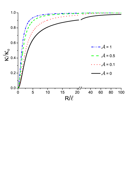
Figure 1: Dependence on the scaled wire radius, $R/\ell$, of the scaled thermal conductivity, $\kappa/\kappa_{0}$, for several values of the reflection coefficient $\mathcal{A}$ and $\ell^{2}=s^{2}\theta_{h}\theta_{I_{h}}$, after Ref. [31].

The phonons’ thermal conductivity is strongly affected by the value of the radius of the cylinder in the nanometer domain. In Fig. 1 it is shown such dependence. Parameter $\ell$, with dimensions of length, is a characteristic length, with $\ell^{2}=s^{2}\theta_{h}\theta_{I_{h}}$, that is, in a Debye model, its square is given by the square of the sound velocity times the product of Maxwell times associated to the phonons energy density and energy flux. Figure 1 tells us that there follows a drastic reduction in thermal conductivity for $R/\ell$ below the value 10, and becoming orders of magnitude smaller for $R/\ell<1$. We may then state that in the range of values of $R/\ell$ there exists a threshold below which the sample size (radius of the cylinder in units of $\ell$) leads to a notable reduction of the thermal conductivity, and large increase of the figure-of-merit in thermo-electric engineering. Figure 1 provides information on the influence of the reflection effect at the side boundaries: as expected with increasing reflection coefficient $\mathcal{A}$ there follows an increase in thermal conductivity. It must be noticed that we have considered normal reflection at an smooth surface, but the surface is always rugous with characteristics fractal on average [39] what affects the reflection processes.

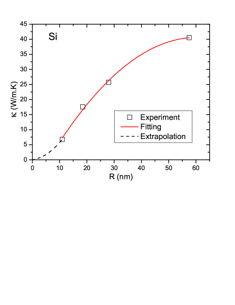
Figure 2: Measured thermal conductivity $\kappa$ of wires of Si in terms of the radius of the wire $R$, at 300 Kelvin; experimental results ($\Box$) from Ref. [50]; after Ref. [31].

Taking into account the experimental data reported by D. Li et al. (Fig. 1(a) in Ref. [50], where it is shown the measured thermal conductivity of silicon in terms of the temperature) in samples of Si nanowires with different diameters (diameters of 22; 37; 56; and 115 nm), we consider those at 300 Kelvin, what is shown in Fig. 2. If we admit that for all the four samples $\kappa_{0}$ is approximately the same and of the order of the thermal conductivity in bulk, namely $\kappa_{0}\simeq$ 148 (W/K.m) [51], we can obtain the values of $\kappa/\kappa_{0}$ given in Table I (third column), and from Fig. 1 (for $\mathcal{A}=0$, i.e., no reflection at the lateral borders: Couette-like flow) we can evaluate that, roughly, the corresponding values of $R/\ell$ are those given in the fourth column, and from them we can estimate the values of $\ell$ shown in the fifth column. Considering as similar the Maxwell times for energy and its flux, which are equal in a Debye model, that is, $\theta_{h}=\theta_{I}=\theta$, we get that $\sqrt{3}\ell/s\approx\theta$, and taking an average sound velocity of 8433 m/s, we obtain the values for the Maxwell time displayed in column 6 of Table I. The experimental data (open square dots) in Fig. 2 are contained in the curve (full line) adjusted by the second order polynomial

$$\kappa\simeq-0.014R^{2}+1.65R-9.31\,,$$

for $R>$ 10 nm. The traced line for $R<$ 10 nm is an intuitive extrapolated indication, given by: $\kappa\simeq 0.045R^{2}+0.122R$.

Table 1: Results for Si

$R$ (nm)	$\kappa$ (W/K.m)	$\kappa/\kappa_{0}$	$R/\ell$	$\ell$ (nm)	$\theta$ (ps)
11.0	6.76	0.046	0.626	17.57	3.61
18.5	17.57	0.119	1.063	17.40	3.57
28.0	25.68	0.173	1.339	20.91	4.29
57.5	40.54	0.274	1.850	31.08	6.38

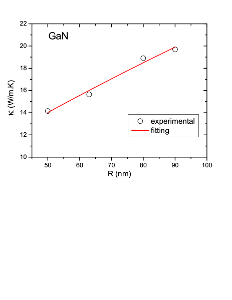
Figure 3: Measured thermal conductivity $\kappa$ of wires of GaN in terms of the radius of the wire $R$, at 300 Kelvin; experimental results ($\bigcirc$) from Ref. [52]; after Ref. [32].

From the experimental data reported by C. Guthy et al. (Fig. 2(a) in Ref. [52], where it is shown the measured thermal conductivity of GaN in terms of the temperature) in GaN nanowires with different diameters (diameters of 100; 126; 160; and 181 nm), we consider those at 300 Kelvin, what is shown in Fig. 3. Using the value of the thermal conductivity in bulk for GaN, namely $\kappa_{0}\simeq$ 210 (W/K.m) [53,54] and taking an average (in this hexagonal crystal) sound velocity of 5170 m/s [52], we obtain, similarly to Table I, the values shown in Table II. The experimental values (open circular dots) in Fig. 3 are contained in the curve (full line) adjusted by the second order polynomial

$$\kappa\simeq-0.0002R^{2}+0.18R+5.7\,,$$

for $R>$ 50 nm.

Table 2: Results for GaN

$R$ (nm)	$\kappa$ (W/K.m)	$\kappa/\kappa_{0}$	$R/\ell$	$\ell$ (nm)	$\theta$ (ps)
50.0	14.1	0.067	0.769	65.0	21.7
63.0	15.6	0.074	0.813	77.5	26.0
80.0	18.9	0.090	0.905	83.4	27.9
90.5	19.7	0.093	0.922	98.1	32.9

It must also be noticed the important point that the characteristic length $\ell$ and Maxwell times depend on $R$ and on the nonequilibrium thermodynamic state of the system. This is so because of their dependence on $R$, which determines the frequencies $\omega_{nq_{z}}$ and of the sum over $nq_{z}$. Figure 4 shows the dependence on the wire radius $R$ of the characteristic length $\ell$ and Maxwell time $\theta$ for GaN and Si nanowires. The linear expressions that relate the characteristic length and Maxwell time with the radius $R$ are indicated within the figures.

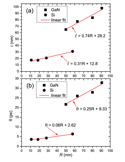
Figure 4: Dependence on the wire radius $R$ of the (a) characteristic length $\ell$ and (b) Maxwell time $\theta$, for GaN and Si nanowires, after Ref. [31].

Concerning the so-called figure of merit, $Z$, which is a number that allows for obtaining a useful insight for optimizing design parameters, is constructed by choosing the parameters that are most centrally vital to a design solution. For the case of thermo-electric devices is used [3]

$$Z=S_{e}\sigma/\kappa\,,$$ (132)

where $S_{e}$ is Seebeck coefficient. If we consider Seebeck effect and the electric conductivity as nearly independent on size, and the phonon thermal conductivity as the relevant one, we can see that, according to the results in figures 1 to 3, the figure of merit $Z$ of Eq. (132) greatly increases in quantum wires with radius in the interval of 10 to 90 nm.

VIII Concluding Remarks

We have presented an extended theory of the Mesoscopic Hydro-Thermodynamics of phonons and carriers in n-doped direct gap polar semiconductors in the presence of electric fields. MHT, also referred to as Higher-Order Generalized Hydrodynamics, extends standard (or Onsagerian) hydrodynamics allowing to incorporate hydrodynamic motion not restricted to smooth in space and time characteristics (i.e., including intermediate to short wavelengths and intermediate to high frequencies). It consists in deriving a set of coupled hydrodynamic equations for the densities of quasi-particles (carriers and phonons) and of energy and their fluxes of all orders. This has been done in Section III.

The matter has been illustrated resorting to a MHT of order 1 for carriers and phonons, which is a contracted description in terms of their densities, energies, and the vectorial fluxes (electric current and heat current) of both. Criteria for performing such contraction are discussed in Ref. [38].

The corresponding four hydrodynamic equations are coupled together, but if we disregard the cross-contributions associated to thermo-electric effects, there follows the separate sets of two equations for the motion of charges and two equations for the motion of energy. These are the basic Eqs. (69) and (70), and Eqs. (71) and (72), respectively. It may be noticed that in these equations are present the quite important generalizations of Maxwell time. We recall that the origin of Maxwell time goes back to the fundamental article by J.C. Maxwell in 1867, on the dynamical theory of gases and liquids [27], in the strain rate model there presented it is considered as representing the time during which the stresses are damped [28]. Section IV is closed with an interpretation of the several contributions to the hydrodynamic equations.

In Section V the hydrodynamic modes in this MHT of order 1 are derived. They allow to characterize the two regimes that are covered by it, namely, a diffusive motion at low wavenumbers and a damped wave motion at intermediate wavenumbers. In the first case the motion is governed by a typical diffusion equation (Fick’s and Fourier’s type respectively), and in the second by a Maxwell-Cattaneo-like equation. A cut-off wavenumber, $Q_{\mathrm{co}}$ of Eq. (100), defines the frontier between the two types of regimes.

Charge motion and characterization of the electric conductivity in the steady state are analyzed in Section VI. It may be notice that at no too small nanometric sizes the conductivity is nearly constant and taking a Drude-type expression. Minor space-dependent effects may result from the presence of the space-dependent distribution of impurities, imperfections, influence of weldings, and boundary conditions (which have a ruggedness of a fractal-on-average type). As noticed at the closing of Section VI, the results can not be extrapolated to wires with very short nanometer radius, say, below a few tenths of nanometers.

Heat motion and characterization of the thermal conductivity in the steady state are analyzed in Section VIII. In the case of the carriers, as it happens with the electric conductivity, the thermal conductivity is constant with an expression of the type of standard kinetic theory, and taking into account the expression for the electric conductivity there follows a type of Wiederman-Franz law. In the case of the phonons, quite differently, there follows a strong space dependence affected by the value of the radius of the wire. There follows a drastic reduction in the thermal conductivity as the radius decreases, evidenced within this MHT of order 1, which is being suppressed if one resorts to standard hydrodynamics. This may be interpreted that as the radius decreases to the nanometric scale larger wavenumbers need be included for the proper description of the movement. A MHT of higher order than 1, would be required for wires with radius of a few nanometers.

Finally, as a consequence of those results we can draw the attention to the fact that the so-called figure of merit in the engineering of thermo-electric devices would greatly increase following the decrease of the wire’s radius.

Acknowledgments: The authors would like to acknowledge partial financial support received from the São Paulo State Research Agency (FAPESP), Goiás State Research Agency (FAPEG), the Brazilian National Research Council (CNPq), and the Brazilian Synchroton Source (LNLS) under a scientific collaborations agreement with Unicamp.

In Memoriam: With very sad feelings, we regret to report the passing away of our dear colleague Áurea Rosas Vasconcellos, a genuine, devoted and extremely competent Teacher and Researcher with fervent dedication to Theoretical Physics in the Condensed Matter area, who was a quite important contributor to the development of the present work.

Appendix A The Nonequilibrium Statistical Operator

According to NESEF ([9,11-13,25] with a short overview given in Ref. [32]), the nonequilibrium statistical operator in terms of the basic nonequilibrium variables in sets (8) and (9) is given by

$$\mathcal{R}_{\varepsilon}(t)=\varrho_{\varepsilon}(t)\times\varrho_{B}\;,$$ (133)

where

$$\varrho_{\varepsilon}(t)=\exp\Big{\{}\ln\bar{\varrho}(t,0)-\int\limits_{-\infty}^{t}dt^{\prime}e^{\varepsilon(t^{\prime}-t)}\frac{d}{dt^{\prime}}\ln\bar{\varrho}(t^{\prime},t^{\prime}-t)\Big{\}}\,,$$ (134)

with $\bar{\varrho}(t,0)$ being the auxiliary statistical operator (also called “instantaneous quasi-equilibrium operator”) and

$$\bar{\varrho}(t^{\prime},t^{\prime}-t) = \exp\Big{\{}-\phi(t)-\sum\limits_{\mathbf{k}}F_{\mathbf{k}}(t^{\prime})\hat{n}_{\mathbf{k}}(t^{\prime}-t)-\sum\limits_{\mathbf{k},\mathbf{Q}\neq 0}F_{\mathbf{kQ}}(t^{\prime})\hat{n}_{\mathbf{kQ}}(t^{\prime}-t)$$ (135)

$$-\sum\limits_{\mathbf{q},\gamma}\varphi_{\mathbf{q\gamma}}(t^{\prime})\hat{\nu}_{\mathbf{q\gamma}}(t^{\prime}-t)-\sum\limits_{\begin{subarray}{c}\mathbf{q},\mathbf{Q}\neq 0\\ \gamma\end{subarray}}\varphi_{\mathbf{qQ\gamma}}(t^{\prime})\hat{\nu}_{\mathbf{qQ\gamma}}(t^{\prime}-t)\Big{\}}\;,$$

where $t^{\prime}$ stands for the dependence on the time of the nonequilibrium thermodynamic variables $F$’s and the dynamical microvariables, in Heisenberg representation, depend on ($t^{\prime}-t$). Moreover $\varrho_{B}$ is the canonical distribution of the bath of acoustic phonons in equilibrium at temperature $T_{0}$, and $\phi(t)$ ensuring the normalization plays the role of the logarithm of a nonequilibrium partition function.

We recall that the second term in the exponent in Eq. (A.2) accounts for historicity and irreversibility in the nonequilibrium state of the system. The quantity $\varepsilon$ is a positive infinitesimal that goes to zero after the trace operation in the calculation of averages has been performed. We also recall that

$$\varrho_{\varepsilon}(t)=\bar{\varrho}(t,0)+\varrho_{\varepsilon}^{\prime}(t)\;,$$ (136)

i.e., it has an additive composition property, with a contribution of the instantaneous quasi-equilibrium statistical operator plus the one of $\varrho_{\varepsilon}^{\prime}$ which contains the historicity and produces irreversible evolution.

Appendix B NESEF-Kinetic Theory

The NESEF-based Kinetic Theory of relaxation processes basically consists into taking the average over the nonequilibrium ensemble of Heisenberg (or Hamilton at the classical level) equations of motion of the dynamical operators for the observables, say, $\hat{A}_{j}(\mathbf{r})$, with $j=1,2,...$, (a function over phase space in classical mechanics and Hermitian operator in quantum mechanics) under consideration, i.e.

$$\frac{\partial}{\partial t}A_{j}(\mathbf{r},t)=\frac{\partial}{\partial t}\mathrm{Tr}\{\hat{A}_{j}(\mathbf{r})\varrho_{\varepsilon}(t)\times\varrho_{B}\}=\mathrm{Tr}\left\{\frac{1}{i\hbar}[\hat{A}_{j}(\mathbf{r}),\hat{H}]\varrho_{\varepsilon}(t)\times\varrho_{B}\right\}\,,$$ (137)

which is a manifestation of Ehrenfest Theorem. The practical handling of this NESEF-Kinetic Theory is described in Refs. [9,11-13] and mainly in [26]. The NESEF is a powerful formalism that provides an elegant, practical, and physically clear picture for describing irreversible processes, adequate to deal with a large class of experimental situations, as for example, in semiconductors far-from equilibrium, obtaining good agreement in comparisons with other theoretical and experimental results [55].

Here we briefly notice that the Markovian limit of the kinetic theory is of particular relevance as a result that, for a large class of problems, the interactions involved are weak and the use of this lowest order, second order in the interaction strengths, in the equations of motion constitutes an excellent approximation of good practical value. By means of a different approach, E. B. Davies [56] has shown that in fact the Markovian approach can be validated in the weak coupling (in the interaction) limit.

Explicitly written, the Markovian equations in the kinetic theory are

$$\frac{\partial}{\partial t}A_{j}(\mathbf{r},t)=J_{j}^{(0)}(\mathbf{r},t)+J_{j}^{(1)}(\mathbf{r},t)+J_{j}^{(2)}(\mathbf{r},t),$$ (138)

where, after it is introduced in the Hamiltonian the separation $\hat{H}=\hat{H}_{0}+\hat{H}^{\prime}$, where $\hat{H}_{0}$ stands for the kinetic energy and $\hat{H}^{\prime}$ contains the interaction potential energies present in Eq. (B1), we have that

$$J_{j}^{(0)}(\mathbf{r},t)=\mathrm{Tr}\left\{\frac{1}{i\hbar}[\hat{A}_{j}(\mathbf{r}),\hat{H}_{0}]\bar{\varrho}(t,0)\times\varrho_{R}\right\}\,,$$ (139)

$$J_{j}^{(1)}(\mathbf{r},t)=\mathrm{Tr}\left\{\frac{1}{i\hbar}[\hat{A}_{j}(\mathbf{r}),\hat{H}^{\prime}]\bar{\varrho}(t,0)\times\varrho_{R}\right\}\,,$$ (140)

and $J_{j}^{(2)}(\mathbf{r},t)=$ ${}_{I}J_{j}^{(2)}(\mathbf{r},t)$ $+$ ${}_{II}J_{j}^{(2)}(\mathbf{r},t)$, with

$${}_{I}J_{j}^{(2)}(\mathbf{r},t)=\frac{1}{(i\hbar)^{2}}\int\limits_{-\infty}^{t}dt^{\prime}e^{\varepsilon(t^{\prime}-t)}\mathrm{Tr}\left\{\big{[}\hat{H}^{\prime}(t^{\prime}-t)_{0},[\hat{H}^{\prime},\hat{A}_{j}(\mathbf{r})]\big{]}\bar{\varrho}(t,0)\times\varrho_{R}\right\}\,,$$ (141)

$${}_{II}J_{j}^{(2)}(\mathbf{r},t)=\frac{1}{i\hbar}\sum\limits_{\mathbf{k}}\int\limits_{-\infty}^{t}dt^{\prime}e^{\varepsilon(t^{\prime}-t)}\mathrm{Tr}\left\{[\hat{H}^{\prime},\hat{A}_{k}(\mathbf{r})]\bar{\varrho}(t,0)\times\varrho_{R}\right\}\frac{\delta J_{j}^{(1)}(\mathbf{r},t)}{\delta A_{k}(\mathbf{r},t)}\,,$$ (142)

where $\bar{\varrho}$ is the auxiliary statistical operator of Eq. (A.3) and $\varrho_{R}$ the equilibrium statistical distribution of the thermal bath, and we recall that $J_{j}^{(0)}$ and $J_{j}^{(1)}$, which in Mori’s terminology [57] are called the precession and force terms, are related to the non-dissipative part of the motion, while dissipative effects are accounted for in $J_{j}^{(2)}$ which can be called scattering integrals. Subindex nought indicates evolution in the interaction representation, $\delta$ indicates functional differentiation [44].

Appendix C Summary of Heims-Jaynes Procedure

Given an statistical operator of the form

$$\varrho=\frac{1}{Z}e^{\widehat{A}+\widehat{B}},$$ (143)

where

$$Z=\mathrm{Tr}\big{\{}e^{\widehat{A}+\widehat{B}}\big{\}}\,,$$ (144)

ensures its normalization, and introducing

$$\varrho_{0}=\frac{e^{\widehat{A}}}{\mathrm{Tr}\big{\{}e^{\widehat{A}}\big{\}}}\,,$$ (145)

according to Heims-Jaynes, given an any operator $\widehat{\Theta}$ it follows that

$$\mathrm{Tr}\big{\{}\widehat{\Theta}\varrho\big{\}}=\langle\widehat{\Theta}\rangle_{0}+\sum\limits_{n=1}^{\infty}\langle\widehat{Q}_{n}(\widehat{\Theta}-\langle\widehat{\Theta}\rangle_{0})\rangle\,,$$ (146)

where

$$\langle\widehat{\Theta}\rangle_{0}=\mathrm{Tr}\big{\{}\widehat{\Theta}\varrho_{0}\big{\}}\,,$$ (147)

with

$$\widehat{Q}_{n}=\widehat{S}_{n}-\sum\limits_{k=1}^{n-1}\langle\widehat{Q}_{n}\rangle_{0}\widehat{S}_{n-k}\,,$$ (148)

for $n\geq 2$, and $\widehat{Q}_{0}=\widehat{1}$ and $\widehat{Q}_{1}=\widehat{S}_{1}$,

$$\widehat{S}_{n}=\frac{B^{n}}{n!}\,,\quad\widehat{S}_{0}=\widehat{1}\,.$$ (149)

Equation (C4) consists of the average value of $\widehat{\Theta}$ with $\varrho_{0}$ (that is, only depending on $A$) plus a contribution in the form of a series expansion in powers of $B$. In a first-order approximation we do have that

$$\mathrm{Tr}\big{\{}\widehat{\Theta}\varrho\big{\}}\simeq\langle\widehat{\Theta}\rangle_{0}+\mathrm{Tr}\big{\{}\widehat{B}(\widehat{\Theta}-\langle\widehat{\Theta}\rangle_{0})\varrho_{0}\big{\}}\,.$$ (150)

In Section III we have used that

$$\overline{\varrho}(t,0)=\frac{1}{\overline{Z}(t)}e^{\widehat{A}+\widehat{B}}\;.$$ (151)

where

$$A(t) = F_{n_{e}}(t)\widehat{n}_{e}+\mathbf{F}_{n_{e}}(t)\cdot\widehat{\mathbf{I}}_{n_{e}}+$$ (152)

$$F_{h_{e}}(t)\widehat{h}_{e}+\mathbf{F}_{h_{e}}(t)\cdot\widehat{\mathbf{I}}_{h_{e}}+$$

$$F_{n_{p}}(t)\widehat{n}_{p}+\mathbf{F}_{n_{p}}(t)\cdot\widehat{\mathbf{I}}_{n_{p}}+$$

$$F_{h_{p}}(t)\widehat{h}_{p}+\mathbf{F}_{h_{p}}(t)\cdot\widehat{\mathbf{I}}_{h_{p}}\;,$$

that is, the homogenous part, $\mathbf{Q}\neq 0$, in the exponent of Eq. (48), and $B(t)$ is the inhomogeneous part, meaning the contributions with $\mathbf{Q}\neq 0$, and we have used the first-order (linear in $\widehat{B}$) approximation.

In particular we had that

$$I_{n_{e}}^{[2]}(\mathbf{Q},t)=B_{1e}^{[2]}(t)n_{e}(\mathbf{Q},t)+B_{2e}^{[2]}(t)h_{e}(\mathbf{Q},t)\,,$$ (153)

$$I_{h_{e}}^{[2]}(\mathbf{Q},t)=C_{1e}^{[2]}(t)n_{e}(\mathbf{Q},t)+C_{2e}^{[2]}(t)h_{e}(\mathbf{Q},t)\,,$$ (154)

with tensor $B$ and $C$ given in Eqs. (73) to (76).

On the other hand, for the case of the phonons we do obtain that

$$\nu_{\mathbf{q}}(t)\simeq\overline{\nu}_{\mathbf{q}}(t)-\overline{\nu}_{\mathbf{q}}(t)[1+\overline{\nu}_{\mathbf{q}}(t)][\mathbf{F}_{n}(t)\cdot\nabla_{\mathbf{q}}\omega_{\mathbf{q}}+\mathbf{F}_{h}(t)\cdot\hbar\omega_{\mathbf{q}}\nabla_{\mathbf{q}}\omega_{\mathbf{q}}]\,,$$ (155)

where

$$\overline{\nu}_{\mathbf{q}}(t)=\frac{1}{e^{\{\varphi_{n}(t)+\varphi_{h}(t)\hbar\omega_{\mathbf{q}}\}}-1}\,,$$ (156)

that is, a first order Taylor expansion in $\mathbf{F}_{n}$ and $\mathbf{F}_{h}$ (linear approximation).

Next, resorting to the use of the nonequilibrium equations of state that relate the four nonequilibrium thermodynamic variables to the four basic variables, it follows in first-order Heims-Jaynes expansion that

$$n(\mathbf{Q},t)=\overline{A}_{11}(t)\varphi_{n}(\mathbf{Q},t)+\overline{A}_{12}(t)\varphi_{h}(\mathbf{Q},t)\,,$$ (157)

$$\mathbf{I}_{n}(\mathbf{Q},t)=\overline{A}_{33}^{[2]}(t)\cdot\mathbf{F}_{n}(\mathbf{Q},t)+\overline{A}_{34}^{[2]}(t)\cdot\mathbf{F}_{h}(\mathbf{Q},t)\,,$$ (158)

$$h(\mathbf{Q},t)=\overline{A}_{21}(t)\varphi_{n}(\mathbf{Q},t)+\overline{A}_{22}(t)\varphi_{h}(\mathbf{Q},t)\,,$$ (159)

$$\mathbf{I}_{h}(\mathbf{Q},t)=\overline{A}_{43}^{[2]}(t)\cdot\mathbf{F}_{n}(\mathbf{Q},t)+\overline{A}_{44}^{[2]}(t)\cdot\mathbf{F}_{h}(\mathbf{Q},t)\,,$$ (160)

where $\overline{A}_{11}$, $\overline{A}_{12}$, $\overline{A}_{33}^{[2]}$, $\overline{A}_{34}^{[2]}$, $\overline{A}_{21}$, $\overline{A}_{22}$, $\overline{A}_{34}^{[2]}$ and $\overline{A}_{44}^{[2]}$ are those of Eqs. (C24) to (C29) below, except for the replacement of $\nu_{\mathbf{q}}(t)$ of Eq. (C13) by $\overline{\nu}_{\mathbf{q}}(t)$ of Eq. (C14).

In Eqs. (C15) and (C17) the contributions in $\mathbf{F}_{n}$ and $\mathbf{F}_{h}$ present in Eq. (C13) are null, whereas in Eqs. (C.16) and (C.18) are null the contributions in $\varphi_{n}$ and $\varphi_{h}$. Eqs. (C15) to (C18) constitute a set of linear algebraic equations that can be inverted to obtain the four nonequilibrium thermodynamic variables $\varphi_{n}$, $\varphi_{h}$, $\mathbf{F}_{n}$ and $\mathbf{F}_{h}$, in terms of the basic hydrodynamic quantities, $n$, $h$, $\mathbf{I}_{n}$ and $\mathbf{I}_{h}$.

The second-order fluxes are given by

$$I_{n}^{[2]}(\mathbf{Q},t)=\overline{A}_{33}^{[2]}(t)\varphi_{n}(\mathbf{Q},t)+\overline{A}_{34}^{[2]}(t)\varphi_{h}(\mathbf{Q},t)\,,$$ (161)

$$I_{h}^{[2]}(\mathbf{Q},t)=\overline{A}_{34}^{[2]}(t)\varphi_{n}(\mathbf{Q},t)+\overline{A}_{44}^{[2]}(t)\varphi_{h}(\mathbf{Q},t)\,,$$ (162)

where $\overline{A}_{33}^{[2]}$, $\overline{A}_{34}^{[2]}$ and $\overline{A}_{44}^{[2]}$ are those of Eqs. (C27), (C28) and (C29), except for the replacement of $\nu_{\mathbf{q}}(t)$ of Eq. (C13) by $\overline{\nu}_{\mathbf{q}}(t)$ of Eq. (C14).

On the other hand, introducing the concept of nonequilibrium temperature, better called quasitemperature $T^{\ast}(\mathbf{r},t)$ in the form

$$k_{B}T^{\ast}(\mathbf{r},t)=\frac{1}{\varphi_{h}(\mathbf{r},t)}\,,$$ (163)

we can obtain an evolution equation for it starting with the evolution equation for the energy in the form of the hyperbolic Maxwell-Cattaneo equation, from which together with the nonequilibrium thermodynamic equation of state, Eq. (C17), we have that

$$\left[\sum_{\mathbf{q}}(\hbar\omega_{\mathbf{q}})^{2}\overline{\nu}_{\mathbf{q}}(t)[1+\overline{\nu}_{\mathbf{q}}(t)]\right]\left[\frac{\partial^{2}\varphi_{h}(\mathbf{r},t)}{\partial t^{2}}+\left(\theta_{h}^{-1}+\theta_{\mathbf{I}_{h}}^{-1}\right)\frac{\partial\varphi_{h}(\mathbf{r},t)}{\partial t}\right]+\frac{h(\mathbf{r},t)}{\theta_{h}\theta_{\mathbf{I}_{h}}}$$

$$=\nabla\cdot\left[\overline{A}_{43}^{[2]}(t)\frac{\overline{A}_{12}(t)}{\overline{A}_{11}(t)}-\overline{A}_{44}^{[2]}(t)\right]\cdot\nabla\varphi_{h}(\mathbf{r},t)+$$

$$\nabla\cdot\left[\frac{\overline{A}_{34}^{[2]}(t)}{\overline{A}_{11}(t)}\right]\cdot\nabla n(\mathbf{r},t)+\theta_{\mathbf{I}_{h}}^{-1}\mathcal{I}_{h}^{[0]\mathrm{ext.}}(\mathbf{r},t)\,,$$ (164)

and, after introducing the heat capacity

$$C_{V}(t)=k_{B}\sum_{\mathbf{q}}\left(\frac{\hbar\omega_{\mathbf{q}}}{k_{B}T_{0}}\right)^{2}\overline{\nu}_{\mathbf{q}}(t)[1+\overline{\nu}_{\mathbf{q}}(t)]\,,$$ (165)

where $T_{0}$ is the temperature in equilibrium in this linear treatment, and the quantities $A_{ij}$ and $\Delta_{ij}$ are,

$$A_{11}(t)=\sum_{\mathbf{q}}\nu_{\mathbf{q}}(t)[1+\nu_{\mathbf{q}}(t)]\,,$$ (166)

$$A_{12}(t)=A_{21}(t)=\sum_{\mathbf{q}}\nu_{\mathbf{q}}(t)[1+\nu_{\mathbf{q}}(t)]\hbar\omega_{\mathbf{q}}\,,$$ (167)

$$A_{22}(t)=\sum_{\mathbf{q}}\nu_{\mathbf{q}}(t)[1+\nu_{\mathbf{q}}(t)](\hbar\omega_{\mathbf{q}})^{2}\,,$$ (168)

$$A_{33}^{[2]}(t)=\sum_{\mathbf{q}}\nu_{\mathbf{q}}(t)[1+\nu_{\mathbf{q}}(t)][\nabla_{\mathbf{q}}\omega\mathbf{{}_{\mathbf{q}}}\nabla_{\mathbf{q}}\omega_{\mathbf{q}}]\,,$$ (169)

$$A_{34}^{[2]}(t)=A_{43}^{[2]}(t)=\sum_{\mathbf{q}}\nu_{\mathbf{q}}(t)[1+\nu_{\mathbf{q}}(t)][\nabla_{\mathbf{q}}\omega_{\mathbf{q}}\nabla_{\mathbf{q}}\omega_{\mathbf{q}}]\hbar\omega_{\mathbf{q}}\,,$$ (170)

$$A_{44}^{[2]}(t)=\sum_{\mathbf{q}}\nu_{\mathbf{q}}(t)[1+\nu_{\mathbf{q}}(t)][\nabla_{\mathbf{q}}\omega_{\mathbf{q}}\nabla_{\mathbf{q}}\omega_{\mathbf{q}}](\hbar\omega_{\mathbf{q}})^{2}\,,$$ (171)

$$\Delta_{12}(t)=A_{11}(t)A_{22}(t)-A_{12}(t)A_{12}(t)\,,$$ (172)

$$\Delta_{34}(t)=A_{33}^{[2]}(t)\odot A_{44}^{[2]}(t)-A_{34}^{[2]}(t)\odot A_{34}^{[2]}(t)\,.$$ (173)

In these expressions, $[\nabla_{\mathbf{q}}\omega_{\mathbf{q}}\nabla_{\mathbf{q}}\omega_{\mathbf{q}}]$ denotes the second order tensor with components $\partial\omega/\partial q_{i}\partial\omega/\partial q_{j}$, while $F^{[2]}\odot G^{[2]}=\sum\limits_{ij}F_{ij}G_{ji}$, with $\odot$ standing for full contracted description.

References

(1) C.G. Rodrigues, A.A.P. Silva, C.A.B. Silva, A.R. Vasconcellos,
J.G. Ramos, R. Luzzi, Braz. J. Phys. 40(1), 63 (2010).
(2) D. Jou, J. Casas-Vazquez, M. Criado-Sancho,
Thermodynamics of Fluids Under Flow (Springer, Berlin,
Germany, 2001).
(3) D.M. Rowe, Thermoelectric Handbook: Macro to Nano
(Taylor and Francis, Boca Raton, USA, 2006).
(4) Yu L. Klimontovich, Statistical Theory of Open Systems: A
Unified Approach to Kinetic Description of Processes in Active Systems,
vol. 1, Kluwer Academic, Dordrecht, The Netherlands (1995).
(11) R. Luzzi, A.R. Vasconcellos, J.G. Ramos, Predictive
Statistical Mechanics: a Non-Equilibrium Ensemble Formalism, Kluwer
Academic, Dordrecht, The Netherlands (2002); and Springer e-Books
Archive.
(12) R. Luzzi, A.R. Vasconcellos, J.G. Ramos, Rivista Nuovo Cimento
29(2), 1-85 (2006).
(13) D.N. Zubarev, V. Morozov, G. Röpke, Statistical
Mechanics of Non Equilibrium Processes, vols. 1 and 2, Academie
Verlag-Wiley VCH, Berlin, Germany (1996).
(14) L. Sklar, Physics and Chance: Philosophical Issues in The
Foundations of Statistical Mechanics, Cambridge Univ. Press,
Cambridge, UK (1993).
(28) L.D. Landau, E.M. Lifshitz, Theory of
Elasticity (Pergamon, London, UK, 1959).
(29) C.A.B. Silva, J.G. Ramos, A.R. Vasconcellos, R. Luzzi, J.
Stat. Phys. 112, 2692 (2011).
(30) C.A.B. Silva, J.G. Ramos, A.R. Vasconcellos, R. Luzzi,
Mesoscopic Hydrothermodynamics: Foundations Within a
Nonequilibrium Statistical Ensemble Formalism, arXiv:1210.7280.
(31) C.G. Rodrigues, A.R. Vasconcellos, R. Luzzi, Eur. Phys. J. B
86, 200 (2013); C.G. Rodrigues, A.R. Vasconcellos, R.
Luzzi, Physica E 60, 50 (2014).
(32) F.S. Vannucchi, A.R. Vasconcellos, R. Luzzi, Int. J. Modern
Phys. B 23, 5283 (2009).
(33) U. Fano, Rev. Mod. Phys. 29, 74 (1957).
(34) N.N. Bogoliubov, Lectures in Quantum Statistics I,
Gordon and Breach, New York, USA (1967).
(36) N. Hugenholtz, Application of Field-Theoretical Methods
to Many-Boson Systems, in 1962 Cargèse Lectures on
Theoretical Physics, M. Lévy Ed., Benjamin, New York, USA
(1963).
(37) R. Balian, Y. Alhassed, H. Reinhardt, Phys. Rep. 131,
1 (1986).
(38) J.G. Ramos, A.R. Vasconcellos, R. Luzzi, J. Chem. Phys.
112, 2692 (2000).
(39) F. Family, T. Vizsek, Eds., Dynamic of
Fractal Surfaces (World Scientific, Singapore, 1994).
(41) C.G. Rodrigues, A.R. Vasconcellos, R. Luzzi, V.N. Freire, J. Phys.: Condens. Matter 19, 346214 (2007).
(42) S.P. Heims, E.T. Jaynes, Rev. Mod. Phys. 34(2), 143 (1962) (see Appendix B in page 164).
(43) C.G. Rodrigues, A.R. Vasconcellos, R. Luzzi, J. Appl. Phys. 113, 113701 (2013)
(44) C.G. Rodrigues, A.R. Vasconcellos, R. Luzzi, J. Appl. Phys. 108, 033716 (2010).
(45) J.G. Ramos, A.R. Vasconcellos, R. Luzzi, Int. J. Quantum Chem. 65, 277 (1997).
(46) R. Courant, D. Hilbert, Methods of Mathematical
Physics (Wiley-Interscience, New York, USA, 1953).
(47) J.M. Ziman, Electrons and Phonons (Claredon, Oxford, UK, 1960).
(48) R. Luzzi, A.R. Vasconcellos, J.G. Ramos, Rivista Nuovo
Cimento 30(3), 95 (2007).
(49) C.G. Rodrigues, A.R. Vasconcellos, R. Luzzi, J. Appl. Phys. 99, 073701 (2006).
(50) D. Li, Y. Wu, P. Kim, L. Shi, P. Yang, A. Majumdar, Appl. Phys.
Lett. 83, 2934 (2003).
(51) M. Asheghi, Y.K. Leung, S.S. Wong, K.E. Goodson, Appl. Phys.
Lett. 71, 1798 (1997).
(52) C. Guthy, C-Y Nam, J.E. Fischer, J. Appl. Phys.
103, 64319 (2008).
(53) A. Ježowskia, P. Stachowiaka, T. Suskib, S. Krukowskib, M. Boćkowskib, I.
Grzegoryb, B. Danilchenkoc, Physica B: Condensed Matter
329-333 Part 2, 1531 (2003).
(54) A. Ježowskia, B.A. Danilchenkoc, M. Boćkowskib, I. Grzegoryb, S. Krukowskib,
T. Suskib, T. Paszkiewicz, Solid State Commun. 128, 69
(2003).