Fast separation of two trapped ions

Abstract

We design fast protocols to separate or recombine two ions in a segmented Paul trap. By inverse engineering the time evolution of the trapping potential composed of a harmonic and a quartic term, it is possible to perform these processes in a few microseconds without final excitation. These times are much shorter than the ones reported so far experimentally. The design is based on dynamical invariants and dynamical normal modes. Anharmonicities beyond the harmonic approximation at potential minima are taken into account perturbatively. The stability versus an unknown potential bias is also studied.

I Introduction

Trapped cold ions provide a leading platform to implement quantum information processing. Separating ion chains is in the toolkit of basic operations required. (Merging chains is the corresponding reverse operation so we shall only refer to separation hereafter.) It has been used to implement two-qubit quantum gates processor ; also to purify entangled states entanglement ; entanglement2 , or teleport material qubits teleportation . Moreover, an architecture for processing information scalable to many ions could be developed based on shuttling, separating and merging ion crystals in multisegmented traps kielpinski .

Ion-chain separation is known to be a difficult operation Home . Experiments have progressed towards lower final excitations and shorter times but much room for improvement still remains Rowe ; Bowler ; Ruster . Problems identified include anomalous heating, so devising short-time protocols via shortcuts to adiabaticity (STA) techniques was proposed as a way-out worth exploring Kaufmann . STA methods intend to speed up different adiabatic operations Xi ; Review without inducing final excitations. An example of an elementary (fast quasi-adiabatic) STA approach Xi was already applied for fast chain splitting in Bowler . Here, we design, using a more general and efficient STA approach based on dynamical normal modes Palmero ; expansion , protocols to effectively separate two equal ions, initially in a common electrostatic linear harmonic trap, into a final configuration where each ion is in a different well. The motion is assumed to be effectively one dimensional due to tight radial confinement. The external potential for an ion at $q$ is approximated as

$$V_{ext}=\alpha(t)q^{2}+\beta(t)q^{4},$$ (1)

which is experimentally realizable with state-of-art segmented Paul Traps Home ; NH .

Using dynamical normal modes (NM) Palmero ; expansion a Hamiltonian will be set which is separable in a harmonic approximation around potential minima. By means of Lewis-Riesenfeld invariants LR we shall design first the approximate dynamics of an unexcited splitting, taking into account anharmonicities in a perturbative manner, and from that inversely find the corresponding protocol, i.e. the $\alpha(t)$ and $\beta(t)$ functions.

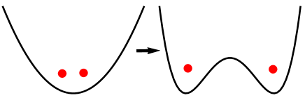
Figure 1: (Color online) Scheme of the separation process. At $t=0$ (left), both ions are trapped within the same external harmonic potential. At final time $t_{f}$ (right), the negative harmonic term, and a quartic term build a double well external potential. The aim of the process is to set each of the ions in a different well without any residual excitation.

The Hamiltonian of the system of two ions of mass $m$ and charge $e$ is, in the laboratory frame,

$$H = \frac{p_{1}^{2}}{2m}+\frac{p_{2}^{2}}{2m}+V,$$

$$V = \alpha(t)(q_{1}^{2}+q_{2}^{2})+\beta(t)(q_{1}^{4}+q_{2}^{4})+\frac{C_{c}}{q_{1}-q_{2}},$$ (2)

where $p_{1},p_{2}$ are the momentum operators for both ions, $q_{1},q_{2}$ their position operators, and $C_{c}=\frac{e^{2}}{4\pi\epsilon_{0}}$, $\epsilon_{0}$ being the vacuum permittivity. We use on purpose a c-number notation since we shall also consider classical simulations. The context will make clear if $c-$numbers or $q-$numbers are required. We suppose that, due to the strong Coulomb repulsion, $q_{1}>q_{2}$. By minimizing the potential part of the Hamiltonian $V$, we find for the equilibrium distance between the two ions, $d(t)$, the quintic equation Home

$$\beta(t)d^{5}(t)+2\alpha(t)d^{3}(t)-2C_{c}=0,$$ (3)

which will be quite useful for inverse engineering the ion-chain splitting, even without an explicit solution for $d(t)$. At $t=0$ a single external well is assumed, $\beta(0)=0$ and $\alpha(0)>0$, whereas in the final double-well configuration $\beta(t_{f})>0,\alpha(t_{f})<0$. At some intermediate time $t_{i}$ the potential becomes purely quartic ($\alpha(t_{i})=0$). Our aim is to design the functions $\alpha(t)$ and $\beta(t)$ so that each of the ions ends up in a different external well as shown in Fig. 1, in times as short as possible, and without any final excitation.

II Dynamical Normal Modes

To define dynamical NM coordinates, we calculate first at equilibrium (the point $\{q_{1}^{(0)},q_{2}^{(0)}\}$ in configuration space where the potential is a minimum, $\partial V/\partial q_{1}=\partial V/\partial q_{2}=0$) the matrix $V_{ij}=\frac{1}{m}\frac{\partial^{2}V}{\partial q_{i}\partial q_{j}}\big{|}_{{}_{\rm{eq}}}$. The equilibrium positions are $q_{1}^{(0)}=\frac{d(t)}{2}$, $q_{2}^{(0)}=-\frac{d(t)}{2}$, and the matrix takes the form

$$V_{ij}=\frac{1}{m}\begin{pmatrix}2\alpha+12\beta\frac{d^{2}}{4}+\frac{2C_{c}}{d^{3}}&-\frac{2C_{c}}{d^{3}}\\ \frac{-2C_{c}}{d^{3}}&2\alpha+12\beta\frac{d^{2}}{4}+\frac{2C_{c}}{d^{3}}\end{pmatrix}.$$ (4)

The eigenvalues are

$$\lambda_{-} = \frac{1}{m}(2\alpha+3\beta d^{2}),$$

$$\lambda_{+} = \frac{1}{m}\left(2\alpha+3\beta d^{2}+\frac{4C_{c}}{d^{3}}\right),$$ (5)

which define the NM frequencies as $\Omega_{\pm}=\sqrt{\lambda_{\pm}}$ corresponding to center-of-mass ($-$) and relative (stretch) motions (+). These relations, with Eq. (3) written as

$$\beta(t)=\frac{2C_{c}}{d^{5}(t)}-\frac{2\alpha(t)}{d^{2}(t)},$$ (6)

allow us to write $\alpha(t)$ and $d(t)$ as functions of the NM frequencies,

$$\alpha(t) = \frac{1}{8}m\left(3\Omega_{+}^{2}-5\Omega_{-}^{2}\right),$$ (7)

$$d(t) = \sqrt[3]{\frac{4C_{c}}{m\left(\Omega_{+}^{2}-\Omega_{-}^{2}\right)}}.$$ (8)

Substituting these expressions into Eq. (6), $\beta(t)$ may also be written in terms of NM frequencies.

The normalized eigenvectors are

$$v_{-} = \frac{1}{\sqrt{2}}\binom{1}{1},$$

$$v_{+} = \frac{1}{\sqrt{2}}\binom{1}{-1},$$ (9)

which we denote as $v_{\pm}=\binom{a_{\pm}}{b_{\pm}}$. The (mass weighted) dynamical NM coordinates are defined in terms of the laboratory coordinates as

$${\sf q}_{\pm}=a_{\pm}\sqrt{m}(q_{1}-q_{1}^{(0)})+b_{\pm}\sqrt{m}(q_{2}-q_{2}^{(0)}).$$ (10)

The unitary transformation of coordinates is

$$U=\int d{\sf q}_{+}d{\sf q}_{-}dq_{1}dq_{2}|{\sf q}_{+},{\sf q}_{-}\rangle\langle{\sf q}_{+},{\sf q}_{-}|q_{1},q_{2}\rangle\langle q_{1},q_{2}|,$$ (11)

where $\langle{\sf q}_{+},{\sf q}_{-}|q_{1},q_{2}\rangle=\delta[q_{1}-q_{1}({\sf q}_{+},{\sf q}_{-})]\delta[q_{2}-q_{2}({\sf q}_{+},{\sf q}_{-})]$. The Hamiltonian in the dynamical equation for $|\psi^{\prime}\rangle=U|\psi\rangle$, where $|\psi\rangle$ is the lab-frame time-dependent wave function evolving with $H$, is given by

$$H^{\prime} = UHU^{\dagger}-i\hbar U(\partial_{t}U^{\dagger})=$$ (12)

$$= \frac{{\sf p}_{+}^{2}}{2}+\frac{1}{2}\Omega_{+}^{2}{\sf q}_{+}^{2}+\frac{\dot{d}}{\sqrt{2}}\sqrt{m}{\sf p}_{+}$$

$$+ \frac{{\sf p}_{-}^{2}}{2}+\frac{1}{2}\Omega_{-}^{2}{\sf q}_{-}^{2},$$

plus qubic and higher order terms in the potential that we neglect by now (they will be considered in Sec. IV below). Similarly to Palmero ; expansion , we apply a further unitary transformation $\mathcal{U}=e^{-i\sqrt{m}\dot{d}{\sf q}_{+}/(\sqrt{2}\hbar)}$, to write down an effective Hamiltonian for $|\psi^{\prime\prime}\rangle=\mathcal{U}|\psi^{\prime}\rangle$ with the form of two independent harmonic oscillators in NM space, $H^{\prime\prime}=\mathcal{U}H^{\prime}\mathcal{U}^{\dagger}-i\hbar\mathcal{U}(\partial_{t}\mathcal{U}^{\dagger})$,

$$H^{\prime\prime} = \frac{{\sf p}_{+}^{2}}{2}+\frac{1}{2}\Omega_{+}^{2}\left({\sf q}_{+}+\frac{\sqrt{m}\ddot{d}}{\sqrt{2}\Omega_{+}^{2}}\right)^{2}$$ (13)

$$+ \frac{{\sf p}_{-}^{2}}{2}+\frac{1}{2}\Omega_{-}^{2}{\sf q}_{-}^{2}=H^{\prime\prime}_{+}+H^{\prime\prime}_{-}.$$

These oscillators have dynamical invariants of the form LR

$$I_{\pm} = \frac{1}{2}[\rho_{\pm}({\sf p}_{\pm}-\dot{x}_{\pm})-\dot{\rho}_{\pm}({\sf q}_{\pm}-x_{\pm})]^{2}$$ (14)

$$+ \frac{1}{2}\Omega_{0\pm}^{2}\left(\frac{{\sf q}_{\pm}-x_{\pm}}{\rho_{\pm}}\right)^{2},$$

where the auxiliary functions $\rho_{\pm}$ and $x_{+}$ satisfy

$$\ddot{\rho}_{\pm}+\Omega_{\pm}^{2}\rho_{\pm}=\frac{\Omega_{0\pm}^{2}}{\rho_{\pm}^{3}},$$ (15)

$$\ddot{x}_{+}+\Omega_{+}^{2}x_{+}=-\sqrt{\frac{m}{2}}\ddot{d},$$ (16)

with $\Omega_{0\pm}=\Omega_{\pm}(0)$, and, due to symmetry, $x_{-}=0$.

The physical meaning of the auxiliary functions may be grasped from the solutions of the time-dependent Schrödinger equations (for each NM Hamiltonian $H^{\prime\prime}_{\pm}$ in Eq. (13)) proportional to the invariant eigenvectors Erik . They form a complete basis for the space spanned by each Hamiltonian $H^{\prime\prime}_{\pm}$ and take the form

$$\langle{\sf q}_{\pm}|\psi^{\prime\prime}_{n\pm}(t)\rangle=e^{\frac{i}{\hbar}\left[\frac{\dot{\rho}_{\pm}{\sf q}_{\pm}^{2}}{2\rho_{\pm}}+(\dot{x}_{\pm}\rho_{\pm}-x_{\pm}\dot{\rho}_{\pm})\frac{{\sf q}_{\pm}}{\rho_{\pm}}\right]}\frac{\Phi_{n}(\sigma_{\pm})}{\rho_{\pm}^{1/2}},$$ (17)

where $\sigma_{\pm}=\frac{{\sf q}_{\pm}-x_{\pm}}{\rho_{\pm}}$, and $\Phi_{n}(\sigma_{\pm})$ are the eigenfunctions of the static harmonic oscillator at time $t=0$. Thus $\rho_{\pm}$ are scaling factors proportional to the state “width” in NM coordinates, whereas the $x_{\pm}$ are the dynamical-mode centers in the space of NM coordinates. Within the harmonic approximation there are dynamical states of the factorized form $|\psi^{\prime\prime}(t)\rangle=|\psi^{\prime\prime}_{+}(t)\rangle|\psi^{\prime\prime}_{-}(t)\rangle$ for the ion chain dynamics, where the NM wave functions $|\psi^{\prime\prime}_{\pm}(t)\rangle$ evolve independently with $H^{\prime\prime}_{\pm}$. They may be written as combinations of the form $|\psi^{\prime\prime}_{\pm}(t)\rangle=\sum_{n}C_{n\pm}|\psi^{\prime\prime}_{n\pm}(t)\rangle$, with constant amplitudes $C_{n\pm}$. The average energies of the $n$-th basis states for the two NM are $E^{\prime\prime}_{n\pm}=\langle\psi^{\prime\prime}_{n\pm}|H^{\prime\prime}_{\pm}|\psi^{\prime\prime}_{n\pm}\rangle$,

$$E^{\prime\prime}_{n-} = \frac{(2n+1)\hbar}{4\Omega_{0-}}\left(\dot{\rho}_{-}^{2}+\Omega_{-}^{2}\rho_{-}^{2}+\frac{\Omega_{0-}^{2}}{\rho_{-}^{2}}\right),$$

$$E^{\prime\prime}_{n+} = \frac{(2n+1)\hbar}{4\Omega_{0+}}\left(\dot{\rho}_{+}^{2}+\Omega_{+}^{2}\rho_{+}^{2}+\frac{\Omega_{0+}^{2}}{\rho_{+}^{2}}\right)$$ (18)

$$+ \frac{1}{2}\dot{x}_{+}^{2}+\frac{1}{2}\Omega_{+}^{2}\left(x_{+}-\frac{\sqrt{m}\ddot{d}}{\sqrt{2}\Omega_{+}^{2}}\right)^{2}.$$

III Design of the Control Parameters

Once the Hamiltonian and Lewis-Riesenfeld invariants are defined, we proceed to apply the invariant based inverse engineering technique and design shortcuts to adiabaticity. The results for the simple harmonic oscillator in Xi serve as a reference but have to be extended here since the two modes are not really independent from the perspective of the inverse problem. This is because a unique protocol, i.e., a single set of $\alpha(t)$ and $\beta(t)$ functions has to be designed.

We first set the initial and target values for the control parameters $\alpha(t)$ and $\beta(t)$. At time $t=0$, the external trap -for a single ion- is purely harmonic, with (angular) frequency $\omega_{0}$. From Eq. (II), we find that $\Omega_{-}(0)=\omega_{0}$ and $\Omega_{+}(0)=\sqrt{3}\omega_{0}$. The equilibrium distance is $d(0)=\sqrt[3]{\frac{2C_{c}}{m\omega_{0}^{2}}}$. For the final time, we set a tenfold expansion of the equilibrium distance, $d(t_{f})=10d(0)$, and $\Omega_{-}(t_{f})=\omega_{0}$. This also implies $\Omega_{+}(t_{f})=\sqrt{1.002}\,\omega_{0}\approx\Omega_{-}(t_{f})$, i.e., the final frequencies of both NM are essentially equal, the Coulomb interaction is negligible, and the ions can be considered to oscillate in independent traps.

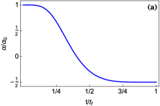
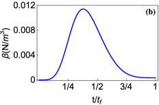
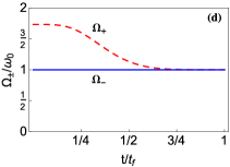
Figure 2: (Color online) Evolution of a) $\alpha(t)$; b) $\beta(t)$; and c) d(t). In d) the NM frequencies, solid line for the ‘-’ and dashed line for the ‘+’ are depicted. Two ⁹Be⁺ ions were separated in the simulation, with $\omega_{0}/(2\pi)=2$ MHz, $t_{f}=5.2$ $\mu$s, $\alpha_{0}=m\omega_{0}^{2}/2$, and $d(0)=5.80$ $\mu$m.

The inverse problem is somewhat similar to the expansion of a trap with two equal ions in Ref. expansion , but complicated by the richer structure of the external potential. The Hamiltonian (13) and the invariant (14) must commute at both boundary times $[H(t_{b}),I(t_{b})]=0$,

$$t_{b}=0,t_{f},$$ (19)

to drive initial levels into final levels via a one-to-one mapping. This is achieved by applying appropriate boundary conditions (BC) to the auxiliary functions $\rho_{\pm}$, $x_{\pm}$ and their derivatives,

$$\rho_{\pm}(0) = 1,\;\;\rho_{\pm}(t_{f})=\gamma_{\pm},$$ (20)

$$\dot{\rho}_{\pm}(t_{b}) = \ddot{\rho}_{\pm}(t_{b})=0,$$ (21)

$$x_{+}(t_{b}) = \dot{x}_{+}(t_{b})=\ddot{x}_{+}(t_{b})=0,$$ (22)

where $\gamma_{\pm}=\sqrt{\frac{\Omega_{\pm}(0)}{\Omega_{\pm}(t_{f})}}$. Let us recall that $x_{-}=0$ for all times so this parameter does not have to be considered further.

Inserting the BC for $x_{+}(t_{b})$ and $\ddot{x}_{+}(t_{b})$ in Eq. (16) we find that $\ddot{d}(t_{b})=0$. Additionally, $\dot{d}(t_{b})=0$ is to be imposed so that ${\mathcal{U}}(t_{b})=1$. According to Eq. (8), $\dot{d}(t_{b})=\ddot{d}(t_{b})=0$ by imposing $\dot{\Omega}_{\pm}(t_{b})=\ddot{\Omega}_{\pm}(t_{b})=0$. With $\dot{d}(t_{b})=\ddot{d}(t_{b})=0$ the Hamiltonians and wave functions coincide at the boundaries, $H^{\prime}(t_{b})=H^{\prime\prime}(t_{b})$, $|\psi^{\prime}(t_{b})\rangle=|\psi^{\prime\prime}(t_{b})\rangle$, which simplifies the calculation of the excitation energy.

From Eq. (15), the NM frequencies may be written as

$$\Omega_{\pm}=\sqrt{\frac{\Omega_{0\pm}^{2}}{\rho_{\pm}^{4}}-\frac{\ddot{\rho}_{\pm}}{\rho_{\pm}}}.$$ (23)

Thus the BC $\dot{\Omega}_{\pm}(t_{b})=\ddot{\Omega}_{\pm}(t_{b})=0$ are satisfied by imposing on the auxiliary functions the additional BC

$$\dddot{\rho}_{\pm}(t_{b})=\ddddot{\rho}_{\pm}(t_{b})=0.$$ (24)

We may now design ansatzes for the auxiliary functions $\rho_{\pm}$ that satisfy the ten BC in Eqs. (20,21,24), plus the BC for $x_{+}(t_{b})$ and $\dot{x}_{+}(t_{b})$ in Eq. (22) (since $\ddot{d}(t_{b})=0$, $\ddot{x}_{+}(t_{b})=0$ is then automatically satisfied, see Eq. (16)). Finally, from the NM frequencies given by Eq. (23) we can inverse engineer the control parameters $\alpha(t)$ and $\beta(t)$ from Eqs. (7,8) and (6).

A simple choice for $\rho_{-}(t)$ is a polynomial ansatz of 9th order $\rho_{-}=\sum_{i=0}^{9}b_{i}s^{i}$, where $s={t}/{t_{f}}$. Substituting this form in the ten BC in Eqs. (20,21,24), we finally get

$$\rho_{-} = 126(\gamma_{-}-1)s^{5}-420(\gamma_{-}-1)s^{6}+540(\gamma_{-}-1)s^{7}$$ (25)

$$- 315(\gamma_{-}-1)s^{8}+70(\gamma_{-}-1)s^{9}+1.$$

For $\rho_{+}$ we will use an 11-th order polynomial $\rho_{+}=\sum_{n=0}^{11}a_{n}s^{n}$ to satisfy as well $x_{+}(t_{b})=\dot{x}_{+}(t_{b})=0$. The parameters $a_{0-9}$ are fixed so that the 10 BC for $\rho_{+}$ are fulfilled (see the Appendix), whereas $a_{10}$, $a_{11}$ are left free, and will be numerically determined by a shooting program Shooting (‘fminsearch’ in MATLAB which uses the Nelder-Mead simplex method for optimization), so that the remaining BC for $x_{+}(t_{b})$ and $\dot{x}_{+}(t_{b})$ are also satisfied. Specifically, for each pair $\{a_{10},a_{11}\}$, $\Omega_{\pm}(t)$ and $d(t)$ are determined from Eqs. (15) and (8), to solve Eq. (16) for $x_{+}(t)$ with initial conditions $x_{+}(0)=\dot{x}_{+}(0)=0$. The free constants are changed until $x_{+}(t_{f})=0$ and $\dot{x}_{+}(t_{f})=0\,$ are satisfied. Numerically a convenient way to find the solution is to minimize the energy $E^{\prime\prime}_{n+}(t_{f})$ in Eq. (II).

Fig. 2 (a) and (b) depict the control parameters $\alpha(t)$ and $\beta(t)$ found with this method, using Eqs. (7) and (6), for some value of $t_{f}$ and $\omega_{0}$, see the caption, while Fig. 2 (c) represents the equilibrium distance between ions as a function of time (8), and Fig. 2 (d) the NM frequencies. In Fig. 3 (a) the excitation energy is shown, versus final time, for optimized parameters given in Fig. 3 (b). The initial state is the ground state of the two ions. It is calculated with an “imaginary time evolution”. This is a variation of any numerical time evolution method (here we used a variation of the split-operator method), where instead of the real time one defines imaginary time in the evolution operator. By letting an ansatz wave function evolve for the static initial potential, it will eventually converge to the ground state of the system. The excitation energy is $E_{ex}=E(t_{f})-E_{0}(t_{f})$, where $E(t_{f})$ is the final energy, calculated in the lab frame, and $E_{0}(t_{f})$ is the final ground-state energy. The wave function evolution is calculated using the “Split-Operator Method” with the full Hamiltonian (I). If the harmonic approximation were exact, there would not be any excitation with this STA method, $E(t_{f})=E^{\prime\prime}_{0+}(t_{f})+E^{\prime\prime}_{0-}(t_{f})=E_{0}(t_{f})$, see Eq. (II). The actual result is perturbed by the anharmonicities and NM couplings. The final ground state is also calculated with an “imaginary time evolution”. The corresponding final ground state energy is essentially two times a harmonic oscillator ground state energy plus the (negligible) Coulomb repulsion at distance $d(t_{f})$. For the final times of all the examples, as it was noted in previous works Kaufmann ; Palmero ; Palmero2 ; expansion , classical simulations (solving Hamilton’s equations from the equilibrium configuration instead of Schrödinger’s equation) give indistinguishable results in the scale of Figure 3 (a).

The excitation energy in Figure 3(a) (solid line) increases at short times since the harmonic NM approximation fails Palmero ; expansion . However, it goes down rapidly below one excitation quantum at times which are still rather small compared to experimental values used so far Bowler ; Ruster . In the following section we shall apply a perturbative technique to minimize the excitation further.

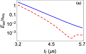
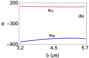
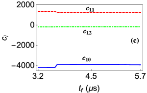
Figure 3: (Color online) a) Final excitation energy vs. final time using the inverse engineering design of Sec. III (solid blue), and the design that takes into account anharmonicities in Sec. IV (dashed red). b) Values of the free parameters $a_{10}$ (solid blue) and $a_{11}$ (dashed red) that minimize the excitation energy for the 11th order polynomial (29). c) Parameters $c_{10}$ (solid blue), $c_{11}$ (dashed red) and $c_{12}$ (dash-dotted green) that minimize the excitation energy for the 12th order polynomial (30). Two ⁹Be⁺ ions where split, with $\omega_{0}/(2\pi)=2$ MHz.

IV Beyond the harmonic approximation

An improvement of the protocol is to consider the perturbation of the higher order terms neglected in the Hamiltonian (13). These “anharmonicities” Morigi are cubic and higher order terms in the Taylor expansion of the Coulomb term ${C_{c}}/({q_{1}-q_{2}})$,

$$\delta V = \sum_{j=3}^{\infty}\delta V^{(j)}$$ (26)

$$= \sum_{j=3}^{\infty}\!\frac{(-1)^{j}C_{c}}{d^{j+1}}\!\left[\!\left(q_{2}-q_{2}^{(0)}\right)\!-\!\left(q_{1}-q_{1}^{(0)}\right)\!\right]^{j}.$$

In NM coordinates the terms take the simple form

$$\delta V^{(j)}=(-1)^{j+1}\frac{C_{c}}{d^{j+1}}\left(\sqrt{\frac{2}{m}}{\sf q}_{+}\right)^{j},$$ (27)

which may be regarded as a perturbation to be added to $H^{\prime\prime}_{+}$ in Eq. (13). (The perturbation does not couple the center-of-mass and relative subspaces.) To first order, the excess energy due to these perturbative terms at final time is given by

$$\delta E_{n+}^{(j)}=\langle\psi^{\prime\prime}_{n+}(t_{f})|\delta V^{(j)}|\psi^{\prime\prime}_{n+}(t_{f})\rangle,$$ (28)

where the $|\psi^{\prime\prime}_{n+}\rangle$ are the unperturbed states in Eq. (17). Inverse engineering the splitting process may now be carried out by considering a 12th order polynomial for $\rho_{+}$ (see (30)), with three free parameters so as to fix the BC for $x_{+}$ and also minimize the excitation energy. In practice we use MATLAB’s ‘fminsearch’ function for the shooting to minimize $E_{0+}(t_{f})+\delta E_{0+}^{(3)}$ as no significant improvement occurs by including higher order terms. Fig. 3 (a) compares the performance of such a protocol with the simpler one with the 11th-order polynomial (29). Fig. 3 (c) gives the values of optimized parameters at different final times.

V Discussion

A large quartic potential is desirable to control the excitations produced at the point where the harmonic term changes its sign Kaufmann . At this point, the harmonic potential switches from confining to repulsive, which reduces the control of the system and potentially increases diabaticities and heating. In the inverse approach proposed here there is no special design of the protocol at this point, but the method naturally seeks high quartic confinements there. In Fig. 2 (b) $\beta$ reaches its maximum value right at the time where $\alpha$ changes sign (see Fig. 2 (a)). However, the maximum value that $\beta$ can reach will typically be limited in a Paul trap Home . In Table 1 we summarize the different maximal values of $\beta$ and critical times (final times at which excitations below 0.1 quanta are reached) for different values of $\omega_{0}$ using the 11-th order polynomial (29) for $\rho_{+}$.

$\omega_{0}$ (MHz)	$\beta_{max}$ ($10^{-3}$N/m3)	$t_{crit}$ ($\mu$s)
3	44.2	2.9
2	11.4	4.4
1.2	2.082	7.4
0.8	0.539	11.2

Table 1: Maximum values of $\beta$, and critical times (final times at which excitations below 0.1 quanta are reached) for different values of $\omega_{0}$. The calculations were performed with the 11-th order polynomial for $\rho_{+}$.

The maximum $\beta$ decreases with $t_{f}$, such that the shortest possible $t_{f}$ at a given maximum tolerable excitation energy is limited by the achievable $\beta$. The trap used in Ref. Ruster yields a maximum $\beta$ of about $10^{-4}$ N/m³, at $\pm 10$ V steering range. In a recent experiment reported in Wilson , where although the purpose was not ion separation a double well potential was produced, the value used was $\beta\approx 5\times 10^{-3}$ N/m³. The numbers reported in the Table are thus within reach, as the $\beta$ coefficients scale with the inverse 4th power of the overall trap dimension, and technological improvements on arbitrary waveform generators may allow for operation at an increased voltage range.

Another potential limitation the method could encounter in the laboratory is due to biases (a linear slope) in the trapping potential, $V_{ext}=\alpha q^{2}+\beta q^{4}+\lambda q$, with $\lambda$ constant and unknown Kaufmann . Fig. 4 represents the excitation energy versus the energy difference between the two final minima of the external potential, $\Delta E$ (also vs. $\lambda$). To calculate the results, $\alpha(t)$ and $\beta(t)$ are designed as if $\lambda=0$, but the dynamics is carried out with a non-zero $\lambda$, in particular the initial state is the actual ground state, including the perturbation. Note that $\Delta E$ should be more than a thousand vibrational quanta to excite the final energy by one quantum. In Ref. Ruster an energy increase of ten phonons at about 150 zN and 80 $\mu$s separation time was reported, so the STA ramps definitely improve the robustness against bias.

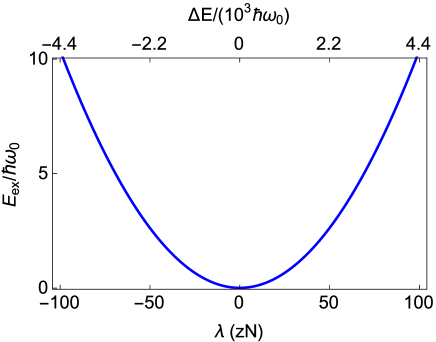
Figure 4: (Color online) Excitation energy vs. different tilt values of the external potential in terms of the energy difference between both wells (upper axis) and values of the $\lambda$ parameter (lower axis), when using the 11-th order polynomial in the evolution. Same parameters as in Fig. 2.

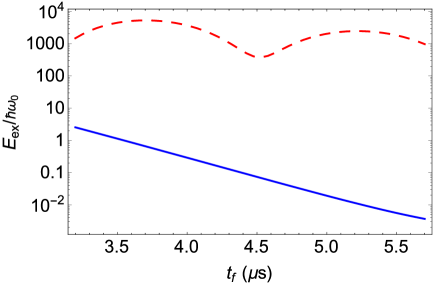
Figure 5: (Color online) Excitation energy vs. final time comparing the 11-th order polynomial (solid blue) and a non optimized trajectory experimentally used in Ruster (dashed red) in the evolution. Same parameters as in Fig. 2.

Further experimental limitations may be due to random fluctuations in the potential parameters, or higher order terms in the external potential. We leave these important issues for a separate study but note that the structure of the STA techniques used here is well adapted to deal with noise or perturbations Andreas ; Xiao1 ; Xiao2 .

Finally, we compare in Fig. 5 the performance of the protocols based on the polynomials (25) and (29) with a simple non-optimized protocol based on those experimentally used in Ruster . There, the equilibrium distance $d$ is first designed as $d(t)=d(0)+[d(t_{f})-d(0)]s^{2}\sin(s\pi/2)$, where $s=t/t_{f}$. From the family of possible potential ramps consistent with this function, we chose a polynomial that drives $\alpha$ from $\alpha(0)=\alpha_{0}$ to $\alpha(t_{f})=-\alpha_{0}/2$ (as in Fig. 2) and whose first derivatives are 0 at both boundary times. $\beta$ is given by Eq. (3). For the times analysed in Fig. 5, the method based on Eqs. (25) and (29) clearly outperforms the non-optimized ramp. To get excitations below the single motional excitation quantum with the non-optimized protocol, final times as long as $t_{f}\sim 80\,\mu$s would be needed, which is in line with current experiments.

We conclude that the method presented here, could bring a clear improvement with respect to the best results experimentally reported so far Bowler ; Ruster . The parameters required are realistic in current trapped ions laboratories. The simulations show that, under ideal conditions, the separation of two ions could be performed in a few oscillation periods, at times similar to those required for other operations as transport Palmero or expansions expansion , also studied with STA.

Appendix A Ansatz for $\rho_{+}$

The ansatz for $\rho_{+}$ that satisfies the BC $\rho_{+}(0)=1$, $\rho_{+}(t_{f})=\gamma_{+}$, $\dot{\rho}_{+}(t_{b})=\ddot{\rho}_{+}(t_{b})=\dddot{\rho}_{+}(t_{b})=\ddddot{\rho}_{+}(t_{b})=0$ with two free parameters takes the form

$$\rho_{+} = 1-(126-126\gamma_{+}+a_{10}+5a_{11})s^{5}$$ (29)

$$+ (420-420\gamma_{+}+5a_{10}+24a_{11})s^{6}$$

$$- (540-540\gamma_{+}+10a_{10}+45a_{11})s^{7}$$

$$+ (315-315\gamma_{+}+10a_{10}+40a_{11})s^{8}$$

$$- (70-70\gamma_{+}+5a_{10}+15a_{11})s^{9}$$

$$+ a_{10}s^{10}+a_{11}s^{11}.$$

To minimize the perturbation energy in Eq. (28), three free parameters are introduced,

$$\rho_{+} = 1-(126-126\gamma_{+}+c_{10}+5c_{11}+15c_{12})s^{5}$$ (30)

$$+ (420-420\gamma_{+}+5c_{10}+24c_{11}+70c_{12})s^{6}$$

$$- (540-540\gamma_{+}+10c_{10}+45c_{11}+126c_{12})s^{7}$$

$$+ (315-315\gamma_{+}+10c_{10}+40c_{11}+105c_{12})s^{8}$$

$$- (70-70\gamma_{+}+5c_{10}+15c_{11}+35c_{12})s^{9}$$

$$+ c_{10}s^{10}+c_{11}s^{11}+c_{12}s^{12}.$$

References

- (1) Hanneke D, Home J P, Jost J D, Amini J M, Leibfried D and Wineland D J 2010 Realisation of a programmable quantum information processor Nat. Phys. 6 13
- (2) Reichle R, Leibfried D, Knill E, Britton J, Blakestad R B, Jost J D, Langer C, Ozeri R, Seidelin S and Wineland D J, 2006 Experimental purification of two-atom entanglement Nature (London) 443 838
- (3) Jost J D, Home J P, Amini J M, Hanneke D, Ozeri R, Langer C, Bollinger J J, Leibfried D and Wineland D J, 2009 Entangled Mechanical Oscillators Nature (London) 459 683
- (4) Barrett M D, Chiaverini J, Schaetz T, Britton J, Itano W M, Jost J D, Knill E, Langer C, Ozeri R and Wineland D J 2004 Deterministic quantum teleportation of atomic qubits Nature (London) 429 737
- (5) Kielpinski D, Monroe C and Wineland D J 2002 Architecture for a Large-Scale Ion-Trap Quantum Computer Nature (London) 417 709
- (6) J. P. Home and A. M. Steane. 2006 Electrode Configurations for Fast Separation of Trapped Ions Quantum Inf. Comput. 6 289-325
- (7) Bowler R, Gaebler J P, Lin Y, T. R. Tan, Hanneke D, Jost J D, Home J P, Leibfried D and Wineland D J 2012 Coherent Diabatic Transport and Separation in a Multi-zone Trap Array Phys. Rev. Lett. 109 080502
- (8) Ruster T, Warschburger C, Kaufmann H, Schmiegelow C T, Walther A, Hettrich M, Pfister A, Kaushal V, Schmidt-Kaler F and Poschinger U G 2014 Experimental realization of fast ion separation in segmented Paul traps Phys. Rev. A 90 033410
- (9) Rowe M A, Ben-Kish A, DeMarco B, Leibfried D, Meyer V, Beall J, Britton J, Hughes J, Itano W M, Jelenkovic B, Langer C, Rosenband T and Wineland D J 2002 Transport of quantum states and separation of ions in a dual rf ion trap Quantum Inf. Comput. 2, 257 (2002).
- (10) Kaufmann H, Ruster T, Schmiegelow C T, Schmidt-Kaler F and Poschinger U G 2014 Dynamics and control of fast ion crystal splitting in segmented Paul traps New J. Phys. 16 073012
- (11) Chen X, Ruschhaupt A, Schmidt S, del Campo A, Guéry-Odelin D and Muga J G 2010 Fast Optimal Frictionless Atom Cooling in Harmonic Traps: Shortcut to Adiabaticity Phys. Rev. Lett. 104 063002
- (12) Torrontegui E, Ibáñez S, Martínez-Garaot S, Modugno M, del Campo A, Guéry-Odelin D, Ruschhaupt A, Chen Xi and Muga J G 2013 Shortcuts to adiabaticity Adv. At. Mol. Opt. Phy. 62 117
- (13) Palmero M, Bowler R, Gaebler J P, Leibfried D and Muga J G 2014 Fast transport of mixed-species ion chains within a Paul trap Phys. Rev. A 90 053408
- (14) Palmero M, Martínez-Garaot S, Alonso J, Home J P, and Muga J G Fast expansions and compressions of trapped-ion chains arXiv:1502.00998
- (15) Nizamani A H and Hensinger W K 2012 Optimum electrode configurations for fast ion separation in microfabricated surface ion traps Appl. Phys. B 106 327
- (16) Lewis H R and Riesenfeld W B, 1969 An Exact Quantum Theory of the Time-Dependent Harmonic Oscillator and of a Charged Particle in a Time-Dependent Electromagnetic Field J. Math. Phys. 10 1458
- (17) Press W H, Teukolsky S A, Vetterling W T, Flannery B P 2007 ”Section 18.1. The Shooting Method”. Numerical Recipes: The Art of Scientific Computing (3rd ed.). New York: Cambridge University Press. ISBN 978-0-521-88068-8.
- (18) Palmero M, Torrontegui E, Guéry-Odelin D and Muga J G 2013 Fast transport of two ions in an anharmonic trap Phys. Rev. A 88 053423
- (19) Morigi G and Walther H 2001 Two-species Coulomb chains for quantum information Eur. Phys. J. D 13 261
- (20) Torrontegui E, Chen Xi, Modugno M, Ruschhaupt A, Guéry-Odelin D and Muga J G 2012 Fast transitionless expansion of cold atoms in optical Gaussian-beam traps Phys. Rev. A 85 033605
- (21) Torrontegui E, Ibáñez S, Chen X, Ruschhaupt A, Guéry-Odelin D and Muga J G 2011 Fast atomic transport without vibrational heating Phys. Rev. A 83 013415
- (22) Wilson A C, Colombe Y, Brown K R, Knill E, Leibfried D and Wineland D J 2014Tunable spin-spin interactions and entanglement of ions in separate potential wells Nature 512, 57-60
- (23) Ruschhaupt A, Chen X, Alonso D and Muga J G 2012 Optimally robust shortcuts to population inversion in two-level quantum systems New J. Phys. 14 093040
- (24) Lu X J, Chen X, Ruschhaupt A, Alonso D, Guérin S and Muga J G 2013 Fast and robust population transfer in two-level quantum systems with dephasing noise and/or systematic frequency errors Phys. Rev. A 88 033406
- (25) Lu X J, Muga J G, Chen X, Poschinger U G, Schmidt-Kaler F and Ruschhaupt A 2014 Fast shuttling of a trapped ion in the presence of noise Phys. Rev. A 89 063414