Observing Supermassive Black Holes across cosmic time: from phenomenology to physics

Abstract

In the last decade, a combination of high sensitivity, high spatial resolution observations and of coordinated multi-wavelength surveys has revolutionized our view of extra-galactic black hole (BH) astrophysics. We now know that supermassive black holes reside in the nuclei of almost every galaxy, grow over cosmological times by accreting matter, interact and merge with each other, and in the process liberate enormous amounts of energy that influence dramatically the evolution of the surrounding gas and stars, providing a powerful self-regulatory mechanism for galaxy formation. The different energetic phenomena associated to growing black holes and Active Galactic Nuclei (AGN), their cosmological evolution and the observational techniques used to unveil them, are the subject of this chapter. In particular, I will focus my attention on the connection between the theory of high-energy astrophysical processes giving rise to the observed emission in AGN, the observable imprints they leave at different wavelengths, and the methods used to uncover them in a statistically robust way. I will show how such a combined effort of theorists and observers have led us to unveil most of the SMBH growth over a large fraction of the age of the Universe, but that nagging uncertainties remain, preventing us from fully understating the exact role of black holes in the complex process of galaxy and large-scale structure formation, assembly and evolution.

1 Introduction

Astrophysical black holes in the local Universe have been inferred to reside in two main classes of systems: X-ray binaries and active galactic nuclei (AGN). Gathering estimates of their masses (either directly via dynamical measurements, or indirectly, using phenomenological relations) allows their mass function to be derived (Shankar et al., 2004; Özel et al., 2010; Kormendy & Ho, 2013). This appears clearly bi-modal, lacking any evidence of a substantial black hole population at intermediate masses (i.e. between $\approx 10^{2}$ and $10^{5}M_{\odot}$). While the height, width and exact mass scale of the low-mass peak can be modeled theoretically as the end-product of stellar (and binary) evolution, and of the physical processes that make supernovae and gamma-ray bursts explode, the supermassive black hole peak in this distribution is the outcome of the cosmological growth of structures and of the evolution of mass inflow towards (and within) the nuclear regions of galaxies, likely modulated by the mergers these nuclear black holes will experience as a result of the hierarchical galaxy-galaxy coalescences.

The main question we are interested in here is the following: given the observed population of supermassive black holes in galactic nuclei, can we constrain models of their cosmological evolution to trace back this local population to their formation mechanisms and the main observable phases of growth, as identified by the entire AGN population?

As opposed to the case of galaxies, where the direct relationship between the evolving mass functions of the various galaxy types and the star formation distribution is not straightforward due to their never-ending morphological and photometric transformation, the case of SMBH is much simpler. By their very nature, black holes are simple (’hairless’) objects, characterized only by two physical properties (mass and spin), the evolution of which is regulated by analytical formulae, to the first order functions of the rate of mass accretion onto them. Thus, for any given “seed” black hole population, their full cosmological evolution can be reconstructed, and its end-point directly compared to any local observation, provided that their growth phases are fully sampled observationally.

This motivates ever more complete AGN searches (surveys). The level to which the desired completeness can in practice be achieved depends on the level of our understanding of the physical and electromagnetic processes that take place around accreting black holes. So, we cannot discuss the evolution of supermassive black holes without an in-depth understanding of AGN surveys, and of their results; but at the same time, we cannot understand properly these surveys if we do not understand the physics behind the observed AGN phenomenology.

In this chapter, I review the current state of affairs regarding the study of the evolution of the black hole population in the nuclei of galaxies. I will first (§ 2) describe the observational techniques used to survey the sky in search of signs of black hole activity, and the progresses made on constraining the phenomenological appearance of AGN (§ 2.2). Then, in section 3, I will move from the phenomenological to the physical description of the processes thought to be responsible for the observed Spectral Energy Distribution (SED) in luminous AGN, focusing in particular on the properties of AGN accretion discs (§ 3.1), coronae (§ 3.2), and the IR-emitting dusty obscurer (the so-called “torus”, § 3.3). In section 4 I will present a concise overview of the current state of the art of AGN luminosity function studies at various wavelength, encapsulating our knowledge about the overall population cosmic evolution. The final section (§ 5) is devoted to a general discussion of the so-called Soltan argument, i.e. the method by which we use the evolutionary study of the AGN population to infer additional global physical properties of the process of accretion onto and energy release by supermassive black holes. In particular, I will show how robust limits on the average radiative and kinetic efficiency of such processes can be derived.

A few remarks about this review are in place. First of all, I do not discuss in detail here the physics of relativistic jets in AGN, which carry a negligible fraction of the bolometric output of the accretion process, but can still carry large fractions of the energy released by the accretion process in kinetic form. This is of course a complex and rich subject in itself, and I refer the reader to the recent reviews by Ghisellini (2011), Perlman (2013) and Heinz (2014). Nonetheless, I will include a discussion about radio luminosity function evolution, which is functional to the aim of compiling a census of the kinetic energy output of SMBH over cosmic time. I also do not discuss in any detail the impact growing black holes might have on the larger-scale systems they are embedded in. The generic topic of AGN feedback has been covered by many recent reviews (see e.g. Cattaneo et al., 2009; Fabian, 2012; McNamara & Nulsen, 2012; Merloni & Heinz, 2013), and would definitely deserve more space than is allowed here. Finally, part of the material presented here has been published, in different form, in two recent reviews (Merloni & Heinz, 2013; Gilfanov & Merloni, 2014), and in Merloni et al. (2014).

2 Finding supermassive black holes: surveys, biases, demographics

Accretion onto supermassive black holes at the center of galaxies manifests itself in a wide variety of different phenomena, collectively termed Active Galactic Nuclei. Their luminosity can reach values orders of magnitude larger than the collective radiative output of all stars in a galaxy, as in the case of powerful Quasars (QSO), reaching the Eddington luminosity for black holes of a few billion solar masses, which can be visible at the highest redshift explored ($z>7$). On the other hand, massive black holes in galactic nuclei can be exceedingly faint, like in the case of Sgr A* in the nucleus of the Milky Way, which radiates at less than a billionth of the Eddington luminosity of the $6.4\times 10^{6}$ M_⊙ BH harboured there. Such a wide range in both black hole masses and accretion rates of SMBH results in a wide, complex, observational phenomenology.

The observational characterization of the various accretion components is challenging, because of the uniquely complex multi-scale nature of the problem. Such a complexity greatly affects our ability to extract reliable information on the nature of the accretion processes in AGN and does often introduce severe observational biases, that need to be accounted for when trying to recover the underlying physics from observations at various wavelengths, either of individual objects or of large samples.

Simple order-of-magnitudes evaluations will suffice here. Like any accreting black holes, an AGN releases most of its energy (radiative or kinetic) on the scale of a few Schwarzschild radii ($\sim 10^{-5}$ pc for a $10^{8}$ $M_{\odot}$ BH). However, the mass inflow rate (accretion rate) is determined by the galaxy ISM properties at the location where the gravitational influence of the central black hole starts dominating the dynamics of the intergalactic gas (the so-called Bondi radius), some $10^{5}$ times further out. The broad permitted atomic emission lines that are so prominent in the optical spectra of un-obscured QSOs are produced at $\sim$0.1-1 pc (Broad Line Region, BLR), while, on the parsec scale, and outside the sublimation radius, a dusty, large-scaleheight, possibly clumpy, medium obscures the view of the inner engine (Elitzur, 2008) crucially determining the observational properties of the AGN (Netzer, 2008); on the same scale, powerful star formation might be triggered by the self-gravitational instability of the inflowing gas (Goodman, 2003). Finally, AGN-generated outflows (either in the form of winds or relativistic jets) are observed on galactic scales and well above (from a few to a few hundreds kpc, some $\sim 10^{8}-10^{10}$ times $r_{\rm g}$!), often carrying substantial amounts of energy that could dramatically alter the (thermo-) dynamical state of the inter-stellar and inter-galactic medium.

When facing the daunting task of assessing the cosmological evolution of AGN, i.e. observing and measuring the signs of accretion onto nuclear SMBH within distant galaxies, it is almost impossible to achieve the desired high spatial resolution throughout the electromagnetic spectrum, and one often resorts to less direct means of separating nuclear from galactic light. There is, however, no simple prescription for efficiently performing such a disentanglement: the very existence of scaling relations between black holes and their host galaxies, and the fact that, depending on the specific physical condition of the nuclear region of a galaxy at different stages of its evolution, the amount of matter captured within the Bondi radius can vary enormously, imply that growing black holes will always display a large range of “contrast” with the host galaxy light.

2.1 On the AGN/galaxy contrast in survey data

More specifically, let us consider an AGN with optical B-band luminosity given by $L_{\rm B,AGN}=\lambda L_{\rm Edd}f_{\rm B}$, where we have introduced the Eddington ratio ($\lambda\equiv L_{\rm bol}/L_{\rm Edd}$), and a bolometric correction $f_{\rm B}\equiv L_{\rm B,AGN}/L_{\rm bol}\approx 0.1$ (Richards et al., 2006). Assuming a mean black hole to host galaxy mass ratio of $A_{0}=0.002$, the contrast between nuclear AGN continuum and host galaxy blue light is given by:

$$\frac{L_{\rm B,AGN}}{L_{\rm B,host}}=39\lambda\left(\frac{f_{\rm B}}{0.1}\right)\left(\frac{A_{0}}{0.002}\right)\frac{(M_{*}/L_{\rm B})_{\rm host}}{3(M_{\odot}/L_{\odot})}$$ (1)

Thus, for typical mass-to-light ratios, the AGN will become increasingly diluted by the host stellar light in the rest-frame UV-optical bands at Eddington ratios $\lambda$ smaller than a few per cent.

Similar considerations can be applied to the IR bands, as follows. For simplicity, we use here the Rieke et al. (2009) relation between monochromatic (24$\mu$m) IR luminosity and Star Formation Rate (SFR, expressed in units of solar masses per year): $L_{\rm 24,SFR}\approx 5\times 10^{42}\times{\rm SFR}$, and the Whitaker et al. (2012) analytic expression for the “main sequence” of star forming galaxies: $\log SFR=\alpha(z)*(\log M_{*}-10.5)+\beta(z)$, with $\alpha(z)=0.7-0.13z$ and $\beta(z)=0.38+1.14z-0.19z^{2}$. Then, the rest-frame 24$\mu$m “contrast” between AGN and galaxy-wide star formation ca be written as:

$$\frac{L_{\rm IR,AGN}}{L_{\rm IR,SF}}\approx 160\lambda 10^{-\beta(z)}\left(\frac{f_{24}}{0.1}\right)\left(\frac{A_{0}}{0.002}\right)\left(\frac{M_{*}}{10^{10.5}M_{\odot}}\right)^{1-\alpha(z)}\,,$$ (2)

where we have defined $f_{24}$ the AGN bolometric correction at 24$\mu$m, and $A_{0}$ is here assumed, for simplicity, to be redshift independent. Thus, for a “typical” $10^{8}M_{\odot}$ black holes in a $10^{10.5}M_{\odot}$ main-sequence star-forming host, the IR emission produced by the global star formation within the galaxy dominates over the AGN emission for $\lambda<0.13$, or $\lambda<0.015$, at $z\sim 1$ or $z\approx 0$, respectively.

When considering star-formation induced hard (2-10 keV) X-ray emission, instead, we obtain

$$\frac{L_{\rm X,AGN}}{L_{\rm X,SF}}\approx 10^{5}\lambda 10^{-\beta(z)}\left(\frac{f_{X}}{0.03}\right)\left(\frac{A_{0}}{0.002}\right)\left(\frac{M_{*}}{10^{10.5}M_{\odot}}\right)^{1-\alpha(z)}\,,$$ (3)

where $f_{X}$ the AGN bolometric correction from the 2-10 keV band, and we have used the expression $L_{\rm X,SF}\simeq 2.5\times 10^{39}\times{\rm SFR}$ (Ranalli et al., 2003; Gilfanov et al., 2004): for the same level of SF in a main sequence AGN host, the nuclear AGN emission dominates the hard X-ray flux as long as the accretion rate exceeds $\lambda>2\times 10^{-4}$, or $\lambda>2\times 10^{-5}$, at $z\sim 1$ or $z\approx 0$, respectively.

This has obvious implications for our understanding of selection biases in AGN surveys. It is clear then that the most luminous optical QSOs (i.e. AGN shining at bolometric luminosity larger than a few times 10⁴⁵ erg/s), represent just the simplest case, as their light out-shines the emission from the host galaxy, resulting in point-like emission with peculiar colors. Less luminous, Seyfert-like, AGN will have a global SED with a non-negligible contribution from the stellar light of the host. As a result, unbiased AGN samples extending to lower-luminosities will inevitably have optical-NIR colors spanning a large range of intermediate possibilities between purely accretion-dominated and purely galaxy-dominated. Optical (and, to a large extent, NIR) surveys will easily pick up AGN at high Eddington ratio, and thus, potentially, all members of a relatively homogeneous class of accretors, while deep X-ray (and radio) surveys can circumvent such biases, by detecting and identifying accretion-induced emission in objects of much lower Eddington ratio.

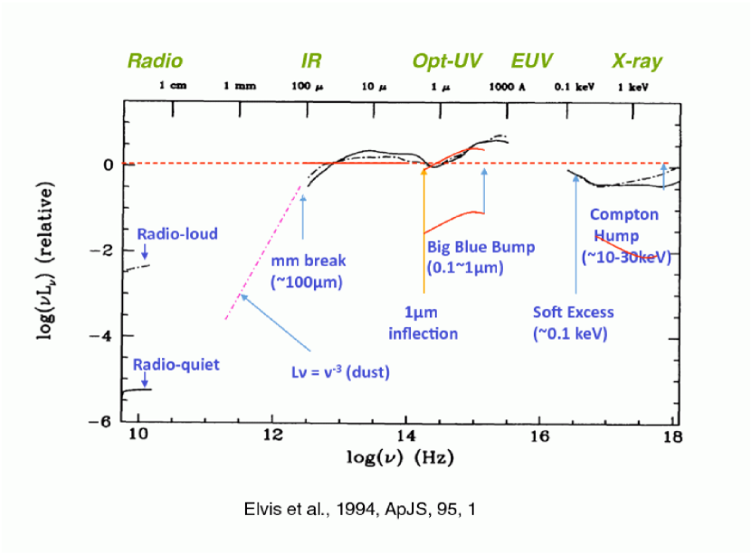
Figure 1: Mean Spectral Energy distribution of UV/X-ray selected quasar from Elvis et al. (1994). Solid black line is for radio-quiet QSOs, dot-dashed for radio-loud.

2.2 Phenomenology of AGN Spectral Energy Distributions

The process of identifying AGN embedded within distant (or nearby) galaxies that we have discussed above is intimately connected with the meticulous work needed to piece together their Spectral Energy Distribution (SED) across the electromagnetic spectrum.

For the practical reasons discussed in the previous section, up until recent years accurate SED of accreting SMBH were constructed mainly from bright un-obscured (type-1) QSO samples. Setting the standard for almost 20 years, the work of Elvis et al. (1994), based on a relatively small number (47) of UV/X-ray selected quasars, has been used extensively as a template for the search and characterization of nearby and distant AGN. The Elvis et al. (1994) SED is dominated by AGN accreting at the highest Eddington ratio, and, as shown in Figure 1, this spectral energy distribution is characterized by a relative flatness across many decades in frequency, with superimposed two prominent broad peaks: one in the UV part of the spectrum (the so-called Big Blue Bump; BBB), one in the Near-IR, separated from an inflection point at about 1$\mu$m.

Subsequent investigations based on large, optically selected QSO samples (most importantly the SDSS one, Richards et al. 2006) have substantially confirmed the picture emerged from the Elvis et al. (1994) study. Apart form a difference in the mean X-ray-to-optical ratio (optically selected samples tend to be more optically bright than X-ray selected ones, as expected), the SDSS quasars have indeed a median SED similar to those shown in fig. 1 for AGN accreting at $L/L_{\rm Edd}>0.1$, despite the difference in redshift and sample size.

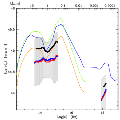
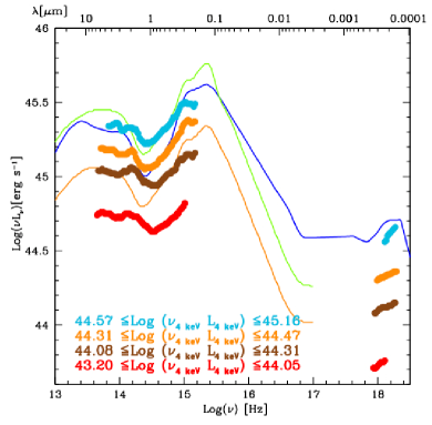
Figure 2: Left Panel: The median (red points) and the mean (blue points) SEDs for the total spectroscopic type-1 COSMOS AGN sample. The mean SED for the “Pure” sample (estimated galaxy contamination $<10$%) is represented with black points. The error bars (gray area) represent the dispersion of the total spectroscopic sample around the mean SED. The average SEDs are compared with the mean SED of Elvis et al. (1994, blue line), the mean SEDs of Richards et al. (2006) using all the SDSS quasar sample (green line) and the near-IR dim SDSS quasar sample (orange line). Right Panel: The median SEDs computed splitting the “Pure” sample in bins of increasing X–ray luminosity at 4 keV. From Lusso (2011)

Large multi-wavelength galaxy survey and extensive follow-up campaigns of medium-wide and deep X-ray surveys (such as the Chandra Deep Field, Giacconi et al. 2002; the COSMOS field, Hasinger et al. 2007; or the X-Bootes field, Hickox et al. 2009) have allowed to extend AGN SED systematic studies to a wide variety of Eddington ratios and AGN/galaxy relative contributions. Figure 2 shows the results of Lusso (2011) (see also Lusso et al. 2010 and Elvis et al. 2012), who analysed an X-ray selected sample of AGN in the COSMOS field, the largest fully identified and redshift complete AGN sample to date. When restricted to a “pure” QSO sample (i.e. one where objects are pre-selected on the basis of a minimal estimated galaxy contamination of $<10$%), the SED of the COSMOS X-ray selected AGN is reminiscent of the Elvis et al. (1994) and Richard et al. (2006) ones, albeit with a less pronounced inflection point at 1$\mu$m. The mean (and median) SED for the whole sample, however, apart from having a lower average luminosity, is also characterized by much less pronounced UV and NIR peaks. This is indeed expected whenever stellar light from the host galaxy is mixed in with the nuclear AGN emission.

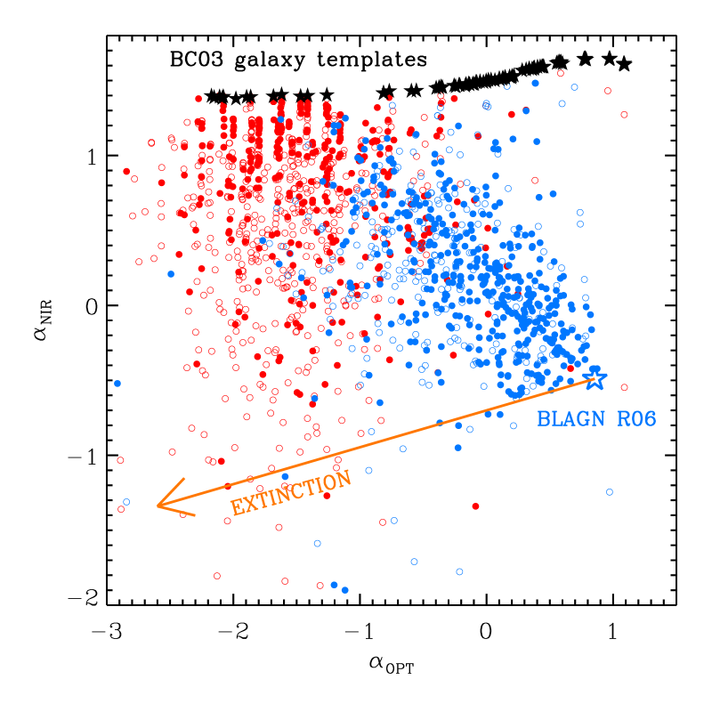
Figure 3: Observed rest-frame SED slopes in the optical ($\alpha_{\rm OPT}$, between 0.3 and 1 $\mu$m) and NIR ($\alpha_{\rm NIR}$ between 1 and 3 $\mu$m) for all ($\sim$1650) X-ray selected AGN in the COSMOS survey. Blue filled circles denote spectroscopically confirmed type 1 (broad lined) AGN, blue empty circles denote candidate type 1 AGN from the photo-z sample. Red filled circles are spectroscopically confirmed type 2 (narrow lined) AGN, empty red circles are candidate type 2 AGN from the photo-z sample. The empty blue star marks the colors of a pure intrinsic type 1 quasar SED (from Richards et al. 2006), while black stars are the loci of synthetic spectral templates of galaxies, with increasing levels of star formation form the left to the right. Nuclear obscuration moves every pure type 1 AGN along the direction of the orange arrow. From Bongiorno et al. (2012).

Figure 3 (Bongiorno et al., 2012; Hao et al., 2012) further illustrates this point. It displays the slope of the rest-frame SED in the optical ($\alpha_{\rm OPT}$, between 0.3 and 1 $\mu$m) and NIR ($\alpha_{\rm NIR}$ between 1 and 3 $\mu$m) bands, i.e. long- and short-wards of the $\sim 1\mu$m inflection point. Pure QSOs, i.e., objects in which the overall SED is dominated by the nuclear (AGN) emission would lie close to the empty blue star in the lower right corner (positive optical slope and negative NIR slope). The location of the X-ray selected AGN in Figure 3 clearly shows instead that, in order to describe the bulk of the population, one needs to consider both the effects of obscuration (moving each pure QSO in the direction of the orange arrow) and an increasing contribution from galactic stellar light (moving the objects towards the black stars in the upper part of the diagram).

3 The spectral components of AGN: accretion discs, coronae and dusty tori

In the previous section, we have presented a phenomenological view of AGN Spectral Energy Distributions, as can be gained by multi-wavelength AGN/QSO surveys, without paying too much attention to the physical origin of the main spectral components themselves. In this section, instead, we analyse the main spectral components of AGN SED, to highlight the connections between AGN phenomenology and physical models of accretion flows.

3.1 AGN accretion discs

The gravitational energy of matter dissipated in the accretion flow around a black hole is primarily converted to photons of UV and soft X-ray wavelengths. The lower limit on the characteristic temperature of the emerging radiation can be estimated assuming the most radiatively efficient configuration: an optically thick accretion flow. Taking into account that the size of the emitting region is $r\sim 10r_{\rm g}$ ($r_{\rm g}=GM_{\rm BH}/c^{2}$ is the gravitational radius) and assuming a black body emission spectrum one obtains:

$$kT_{\rm bb}=\left(\frac{L_{\rm bol}}{\sigma_{\rm SB}\pi r^{2}}\right)^{1/4}\approx 14\left(\frac{L_{\rm bol}}{10^{44}}\right)^{1/4}\left(\frac{M_{\rm BH}}{10^{8}}\right)^{-1/2}{\rm eV}$$ (4)

Proper treatment of the angular momentum transport within the accretion flow allows a full analytical solution of optically thick (but geometrically thin) discs, first discovered by Shakura & Sunyaev (1973). It is a major success of their theory the fact that, for typical AGN masses and luminosities (and thus accretion rates), the expected spectrum of the accretion disc should peak in the optical-UV bands, as observed. Indeed, a primary goal of AGN astrophysics in the last decades has been to model accurately the observed shape of the BBB in terms of standard accretion disc models, and variations thereof.

The task is complicated by at least three main factors. First of all, standard accretion disc theory, as formulated by Shakura & Sunyaev (1973), needs to be supplemented by a description of the disc vertical structure and, in particular, of its atmosphere, in order to accurately predict spectra. This, in turn, depends on the exact nature of viscosity and on the micro-physics of turbulence dissipation within the disc. As in the case of XRB, models for geometrically thin and optically thick AGN accretion discs has been calculated to increasing levels of details, from the simple local blackbody approximation to stellar atmosphere-like models where the vertical structure and the local spectrum are calculated accounting for the major radiative transfer processes (e.g. the TLUSTY code of Hubeny et al. 2000).

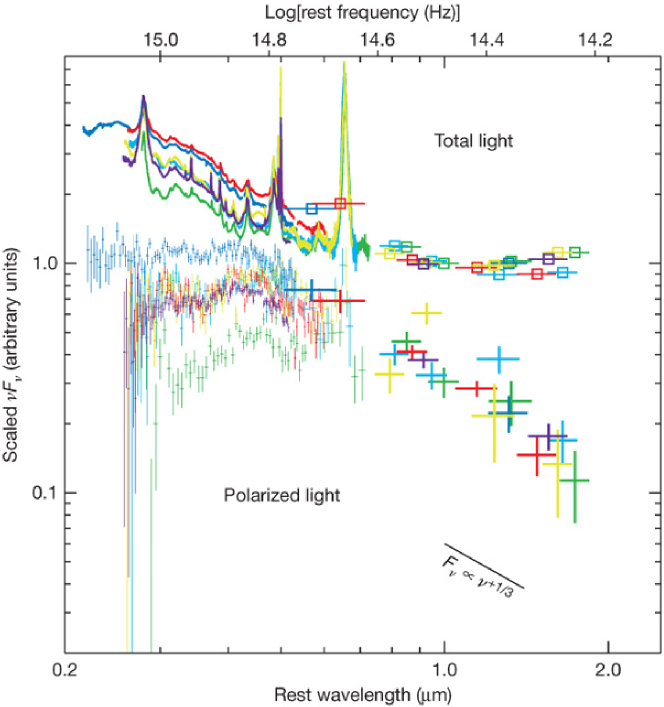
Figure 4: Total-light spectra of nearby QSOs, shown as bold traces in the optical and as squares in the near-infrared, and normalized at 1 $\mu$m in the rest frame. Polarized-light spectra (arbitrarily shifted by a factor of 3 with respect to the total light, for clarity), are shown as light points in the optical and as bold points in the near-infrared, also separately normalized at 1 $\mu$m, by fitting a power law to the near-infrared polarized-light spectra. For both total-light and polarized-light data, horizontal bar lengths indicate bandwidth. The total-light spectra begin to increase in $\nu F_{\nu}$ at wavelengths around, or slightly greater than, 1 $\mu$m. In contrast, the polarized-light spectra all consistently and systematically decrease towards long wavelengths, showing a blue shape of approximately power-law form. From Kishimoto et al. (2008)

A second complicating effect, a purely observational one, is the fact that the intrinsic disc continuum emission is often buried underneath a plethora of permitted atomic emission lines, many of which broadened significantly by gas motions in the vicinity of the central black hole (see, e.g. the solid lines of Figure 4). Interestingly, the metallicities implied by the relative strength of broad emission lines do not show any significant redshift evolution (see Fig. 5): they are solar or super-solar, even in the highest redshift QSOs known (see e.g. Hamann & Ferland, 1992), in contrast with the strong evolution of the metallicity in star forming galaxies.

In particularly favorable geometrical observing conditions, however, by looking at optical spectra in polarised light the “contaminating” broad emission lines are removed, and the true continuum of the accretion disc is revealed. This shows a broad dip possibly corresponding to the Balmer edge absorption expected from an accretion disc atmosphere (Kishimoto et al., 2003). Extending the polarised continuum into the near-IR reveals the classic long wavelength $\nu^{1/3}$ spectrum expected from simple accretion disc models (see Kishimoto et al., 2008, and figure 4).

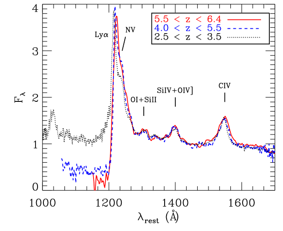
Figure 5: Stacked spectra of quasars in different redshift bins. Note that the relative intensity of the metal lines (and in particular the (SiIV+OIV])$/$CIV ratio) remains constant over the wide redshift interval 2.5$<z<$6.4, indicating that the metallicity in the observed quasars does not evolve with redshift. From Juarez et al. (2009).

Finally, a third complicating factor is that the real physical condition in the inner few hundreds of Schwarzschild radii of an AGN might be more complex than postulated in the standard accretion disc model: for example, density inhomogeneities resulting in cold, thick clouds which reprocess the intrinsic continuum have been considered at various stages as responsible for a number of observed mismatches between the simplest theory and the observations (see e.g. Guilbert & Rees, 1988; Merloni et al., 2006; Lawrence, 2012, and references therein).

Essentially all of the above mentioned problems are particularly severe in the UV part of the spectrum, where observations are most challenging. (Shang et al., 2005) compared broad-band UV-optical accretion disc spectra from observed quasars with accretion disc models. They compiled quasi-simultaneous QSO spectra in the rest-frame energy range 900-9000 $\AA$ and fitted their continuum emission with broken power-law models, and then compared the behavior of the sample to those of non-LTE thin-disk models covering a range in black hole mass, Eddington ratio, disk inclination, and other parameters. The results are far from conclusive: on the one hand, the observed slopes are in general consistent with the expectations of sophisticated accretion disc models. On the other hand, the spectral UV break appears to always be around 1100 $\AA$, and does not scale with the black hole mass in the way expected.

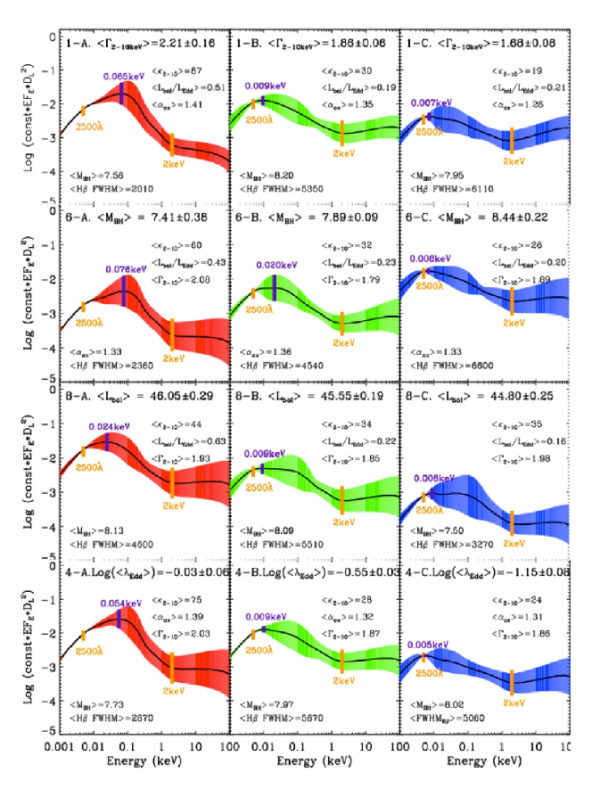
Figure 6: The AGN mean SEDs based on different values of 4 parameters from SED model fitting of AGN (from top to bottom: 2-10 keV X-ray spectral index, black hole mass, bolometric luminosity and Eddington ratio. For each parameter, the 51 sources are sorted according to the parameter value, and re-normalized SED to the mean luminosity at 2500 $\AA$ of. The three panels (A, B, C) in each row show the mean SEDs for the subsets classified by the parameter shown in the panel title. In each panel the solid curve is the mean SED, while the shaded coloured region is the 1$\sigma$ deviation. The peak position of the SED is marked by the vertical solid purple line. The average values of some other parameters in that subset are also shown in the panel. From Jin et al. (2012)

Jin et al. (2012), on the other hand, have looked at detailed continuum fits to the joint optical-UV-X-ray SED of 51 nearby AGN with known black hole masses. Figure  6 shows the variation of the mean SED as a function of various parameters, such as X-ray spectral index $\Gamma_{\rm 2-10}$, black hole mass, bolometric luminosity and Eddington ratio. Clearly, global trends in the basic disc properties (such as its peak temperature) are observed, in correlation with the main parameter of the accretion flow. From a Principal Component analysis, Jin et al (2012) found that the first two eigenvectors contain $\sim 80$% of all correlations in the matrix, with the first one strongly correlating with black hole mass, and the second one with the bolometric luminosity, while both correlate with the Eddington ratio. Interestingly, this turns out to be consistent with the results of a PCA analysis of the emission line-dominated QSO spectra (Boroson, 2002).

Having a well-sampled spectral energy distribution for the AGN emission produced by a standard, Shakura & Sunyaev (1973) accretion disc around a SMBH of known mass, could in principle lead to useful constraints on the overall radiative efficiency of the accretion process, and therefore on the nature of the inner boundary condition of the accretion disc, and on the black hole spin itself.

Davis & Laor (2011) have made a first systematic attempt to estimate the radiative efficiencies of accretion discs in a sample of QSOs. In individual AGN, thin accretion disk model spectral fits can be used to infer the total rate of mass accretion onto the black hole $\dot{M}$, if its mass $M_{\rm BH}$ is known. In fact, by measuring the continuum disk luminosity in the optical band (i.e. in the Rayleigh-Jeans part of the optically thick multi-color disc spectrum), the accretion rate estimates are relatively insensitive to the actual model of the disc atmosphere. The principle is analogous to that employed in black hole X-ray binaries in order to constrain BH spin from the disc continuum measurements (see McClintock et al., 2014), but in a typical AGN, the above-mentioned observational intricacies need to be dealt with, together with the fact that the BBB is much less well sampled than in a stellar mass black hole. On the other hand, the uncertainty in the distance to the object, that plagues the studies of galactic black holes is not an issue for QSOs with measured spectroscopic redshift. Very massive black holes at high redshift have the peak of the disc emission well in the optical bands. Provided one is able to properly correct for the increasing optical depth of the Inter-galactic medium, it could be possible to use simple photometric SED modelling to constrain properties of the disc and the central black hole (see e.g. Ghisellini et al. 2010). At the opposite end of the mass spectrum, small mass black holes accreting at very high rate in the local universe are expected to have such a high disc temperature that the tail of the optically thick thermal emission should appear as “soft excess” in the soft X-ray energy bands. Done et al. (2013) have indeed argued that some Narrow-Line Seyfert 1 galaxies can indeed be modelled with a very high temperature accretion disc, thus gaining information on the disc inner boundary, and, indirectly, on the BH spin.

3.2 AGN coronae and X-ray spectral properties

The upper end of the relevant temperature range reached by accretion flows onto black holes is achieved in the limit of optically thin emission from a hot plasma, possibly analogous to the solar corona, hence the name of accretion disc “coronae” (Galeev et al., 1979). The virial temperature of particles near a black hole, $kT_{\rm vir}=GM_{\rm BH}m/r\propto mc^{2}/(r/r_{\rm g})$, does not depend on the black hole mass, but only on the mass of the particle $m$, being $T_{\rm vir,e}\sim 25(r/10r_{\rm g})^{-1}$ keV for electrons and $T_{\rm vir,p}\sim 46(r/10r_{\rm g})^{-1}$ MeV for protons. As the electrons are the main radiators that determine the emerging spectral energy distribution, while the protons (and ions) are the main energy reservoir, the outcoming radiation temperature for optically thin flows depends sensitively on the detailed micro-physical mechanisms through which ions and electrons exchange their energy in the hot plasma.

Indeed, the values of the electron temperature typically derived from the spectral fits to the hard spectral component in accreting black holes, $kT_{e}\sim 50-150$ keV, are comfortably within the range defined by the two virial temperatures, but, unlike in the case of optically thick accretion solutions, it has proved impossible to derive it from the first principles of accretion theory, and various models have been put forward to explain it (Narayan & Yi, 1994; Blandford & Begelman, 1999).

In most cases, the observed hard X-ray spectral component from hot optically thin plasma is believe to be produced by unsaturated Comptonization of low frequency seed photons from the accretion disc itself (when present), with characteristic temperature $T_{\rm bb}$. Such a spectrum has a nearly power law shape in the energy range from $\sim 3kT_{\rm bb}$ to $\sim kT_{e}$ (Sunyaev & Titarchuk, 1980). For the parameters typical for black holes in AGN this corresponds to the energy range from $\sim$ a few tens of eV to $\sim 50-100$ keV. The photon index $\Gamma$ of the Comptonized spectrum depends in a rather complicated way on the parameters of the Comptonizing media, primarily on the electron temperature and the Thompson optical depth (Sunyaev & Titarchuk, 1980). In fact, the emerging power law slope depends more directly on the Comptonization parameter $y$, which is set by the energy balance in the optically thin medium: critical is the ratio of the energy deposition rate into hot electrons and the energy flux brought into the Comptonization region by soft seed photons (Sunyaev & Titarchuk, 1989; Dermer et al., 1991; Haardt & Maraschi, 1993).

Broadly speaking, significant part of, if not the entire diversity of the spectral behavior observed in accreting black holes of stellar mass can be explained by the changes in the proportions in which the gravitational energy of the accreting matter is dissipated in the optically thick and optically thin parts of the accretion flow. This is less so for supermassive black holes in AGN, where emission sites other than the accretion disk and hot corona may play significant role (e.g.broad and narrow emission line regions or dusty obscuring structures on pc scales, see section 3.1 3.3 above and below). The particular mechanism driving these changes is however unknown. Despite significant progress in MHD simulations of the accretion disk achieved in recent years (Ohsuga & Mineshige, 2011; Schnittman et al., 2013; Jiang et al., 2014) there is no accepted global model of accretion onto a compact object able to fully explain all the different spectral energy distributions observed, nor the transitions among them.

Generically, the X-ray spectra of luminous AGN are all dominated by a power-law in the 2-10 keV energy range, with a relative narrow distribution of slopes: $\langle\Gamma\rangle=1.8\pm 0.2$ (Nandra & Pounds, 1994; Steffen et al., 2006; Young et al., 2009), consistent with the expectations of Comptonization models discussed above, and suggesting a quite robust mechanism is in place to guarantee a almost universal balance between heating and cooling in the hot plasma. Of course, X-ray spectra of AGN are more complex than simple power-laws. A clear reflection component from cold material (George & Fabian, 1991; Reynolds, 1998) is observed in a number of nearby AGN, and further required by Cosmic X-ray Background (CXRB) synthesis models Gilli et al. (2007); and emission and absorption features are also seen in good quality spectra. The most prominent and common of those is a narrow iron K$\alpha$ emission line. Such a line, produced by cold, distant material appears to be dependent on luminosity, with more luminous sources having smaller equivalent widths (the so-called Iwasawa-Taniguchi effect Iwasawa & Taniguchi, 1993).

The physical origin of the tight coupling between cold and hot phases, however, remains elusive. In fact, the main open questions regarding the origin of the X-ray emitting coronae and the reflection component in AGN (and in XRB) are intimately connected with those left open by the classical theory of relativistic accretion discs. The main ones concern a) the physical nature of the viscous stresses and their scaling with local quantities within the disc (pressure, density); b) the exact vertical structure of the disc and the height where most of the dissipation takes place and c) the nature of the inner boundary condition.

As usual, observational hints on the right answers to those questions come more easily from well sampled observations of transient black holes in XRB, where the dynamical evolution of the coupled disc-corona system can be followed in great detail, proving at least a phenomenological framework for how optically thin and optically thick plasma share accretion energy at different accretion rates (Fender et al., 2004).

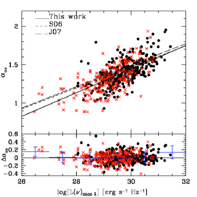
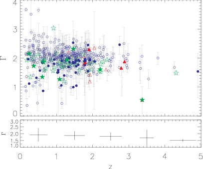
Figure 7: Left: The optical-to-X-ray spectral slope $\alpha_{\rm ox}$ as a function of luminosity density at 2500$\AA$. From Lusso et al. (2010). Right: X-ray photon index ($\Gamma$) vs. redshift $z$. Blue circles represent radio quiet, non-BAL (Broad Absorption Line) quasars, green stars represent radio loud quasars, and red triangles represent BAL quasars. The bottom plot shows the weighted mean $\Gamma$ values for bins of width $\Delta z=1$. No clear sign of evolution in the average X-ray spectral slope of AGN is detected over more than 90% of the age of the universe. From Young et al. (2009).

In the case of AGN, because of the complexities of galactic nuclei discussed above, and because the discs and coronae of AGN emit in distinct parts of the electromagnetic spectrum, it is much more difficult to clearly distinguish between different spectral states in terms of a simple power ratios between the two main spectral components. Nevertheless, as a very general diagnostic, the “X-ray loudness”, usually characterized by the $\alpha_{\rm ox}$ parameter, i.e. the slope of the spectrum between 2500 $\AA\,=5$ eV and 2 keV: $\alpha_{\rm ox}=0.3838\log(F_{\rm 2keV}/F_{\rm 2500})$ can be used to characterize the fraction of bolometric light carried away by high-energy X-ray photons. Recent studies of large samples of both X-ray and optical selected AGN have clearly demonstrated that $\alpha_{\rm ox}$ is itself a function of UV luminosity, with less luminous objects being more X-ray bright (see e.g. Steffen et al., 2006; Lusso et al., 2010; Jin et al., 2012, and the left panel of Figure 7). In very general terms, this might point towards a connection between accretion disc physics and the mechanism(s) of coronae generation in AGN (Merloni, 2003; Wang et al., 2004).

Such generic properties of AGN X-ray SED do not appear to change significantly with redshift: even for the most distant objects known where reliable spectral analysis of AGN can be performed, no clear sign of evolution in either $\alpha_{\rm ox}$ (at fixed luminosity) or the X-ray spectral slope $\Gamma$ has been detected (see the right panel of Figure 7).

3.3 Infrared dust emission from AGN: the link with the nuclear structure at the Bondi radius

The observational appearance of an AGN is not only determined by the intrinsic emission properties of its accretion disc and corona, but also by the nature, amount, dynamical and kinematic state of any intervening material along the line of sight. Intrinsic obscuration does indeed play a fundamental role for our understanding of the overall properties of AGN. As we have seen in the previous section, the intrinsic shape of the X-ray continuum can be characterized by a power-law in the 2-10 keV energy range, with a relative narrow distribution of slopes: $\langle\Gamma\rangle=1.8\pm 0.2$. Thus, the hard slope of the Cosmic X-ray Background (CXRB) spectrum (well described by a power-law with photon index $\Gamma_{\rm CXRB}\simeq 1.4$ at $E<10$ keV), and the prominent peak observed at about 30 keV are best accounted for by assuming that the majority of active galactic nuclei are in fact obscured (Setti & Woltjer, 1989; Comastri et al., 1995, see also Figure 15 below).

In the traditional ’unification by orientation’ schemes, the diversity of AGN observational classes is explained on the basis of the line-of-sight orientation with respect to the axis of rotational symmetry of the system (Antonucci & Miller, 1985; Antonucci, 1993; Urry & Padovani, 1995). In particular, obscured and un-obscured AGN are postulated to be intrinsically the same objects, seen from different angles with respect to a dusty, large-scale, possibly clumpy, parsec-scale medium, which obscures the view of the inner engine (Elitzur, 2008; Netzer, 2008). According to the simplest interpretations of such unification schemes, there should not be any dependence of the obscured AGN fraction with intrinsic luminosity and/or redshift.

However, the results on the statistical properties of obscured AGN from these studies are at odds with the simple ’unification-by-orientation’ scheme. In fact, evidence has been mounting over the years that the fraction of absorbed AGN, defined in different and often independent ways, appears to be lower at higher nuclear luminosities (Lawrence & Elvis, 1982; Ueda et al., 2003; Steffen et al., 2003; Simpson, 2005; Hasinger, 2008; Brusa et al., 2010; Bongiorno et al., 2010; Burlon et al., 2011; Assef et al., 2013; Buchner et al., 2015). Such an evidence, however, is not uncontroversial. As recently summarized by Lawrence & Elvis (2010, and references therein), the luminosity dependence of the obscured AGN fraction, so clearly detected, especially in X-ray selected samples, is less significant in other AGN samples, such as those selected on the basis of their extended, low frequency radio luminosity (Willott et al., 2000) or in mid-IR colors (Lacy et al., 2007). The reasons for these discrepancies are still unclear, with Mayo & Lawrence (2013) arguing for a systematic bias in the X-ray selection due to an incorrect treatment of complex, partially-covered AGN.

Evidence for a redshift evolution of the obscured AGN fraction is even more controversial. Large samples of X-ray selected objects have been used to corroborate claims of positive evolution of the fraction of obscured AGN with increasing redshift (La Franca et al., 2005; Treister & Urry, 2006; Hasinger, 2008), as well as counter-claims of no significant evolution (Ueda et al., 2003; Tozzi et al., 2006; Gilli et al., 2007). More focused investigation on specific AGN sub-samples, such as $z>3$ X-ray selected QSOs (Fiore et al., 2012; Vito et al., 2013), rest-frame hard X-ray selected AGN (Iwasawa et al., 2012), or Compton Thick AGN candidates (Brightman & Ueda, 2012) in the CDFS have also suggested an increase of the incidence of nuclear obscuration towards high redshift. Of critical importance is the ability of disentangling luminosity and redshift effects in (collections of) flux-limited samples and the often complicated selection effects at high redshift, both in terms of source detection and identification/follow-up.

In a complementary approach to these “demographic” studies (in which the incidence of obscuration and the covering fraction of the obscuring medium is gauged statistically on the basis of large populations), SED-based investigations look at the detailed spectral energy distribution of AGN, and at the IR-to-bolometric flux ratio in particular, to infer the covering factor of the obscuring medium in each individual source (Maiolino et al., 2007; Treister et al., 2008; Sazonov et al., 2012; Roseboom et al., 2013; Lusso et al., 2013). These studies also found general trends of decreasing covering factors with increasing nuclear (X-ray or bolometric) luminosity, and little evidence of any redshift evolution (Lusso et al., 2013). Still, the results of these SED-based investigations are not always in quantitative agreement with the demographic ones. This is probably due to the combined effects of the uncertain physical properties (optical depth, geometry and topology) of the obscuring medium (Granato & Danese, 1994; Lusso et al., 2013), as well as the unaccounted for biases in the observed distribution of covering factors for AGN of any given redshift and luminosity (Roseboom et al., 2013). To account for this, different physical models for the obscuring torus have been proposed, all including some form of radiative coupling between the central AGN and the obscuring medium (e.g. Lawrence, 1991; Maiolino et al., 2007; Nenkova et al., 2008).

Irrespective of any specific model, it is clear that a detailed physical assessment of the interplay between AGN fuelling, star formation and obscuration on the physical scales of the obscuring medium is crucial to our understanding of the mutual influence of stellar and black hole mass growth in galactic nuclei (Bianchi et al., 2012). Conceptually, we can identify three distinct spatial regions in the nucleus of a galaxy on the basis of the physical properties of the AGN absorber. The outermost one is the gravitational sphere of influence of the supermassive black hole (SMBH) itself, also called Bondi Radius $R_{\rm B}=2GM_{\rm BH}/\sigma^{2}\simeq 10\,M_{\rm BH,8}\,\sigma_{\rm,300}\;{\rm pc}$, where $M_{\rm BH,8}$ is the black hole mass in units of $10^{8}M_{\odot}$, and $\sigma_{\rm,300}$ can be either the velocity dispersion of stars for a purely collisionless nuclear environment, or the sound speed of the gas just outside $R_{\rm B}$, measured in units of 300 km/s. To simplify, one can consider any absorbing gas on scales larger than the SMBH sphere of influence to be “galactic”, in the sense that its properties are governed by star-formation and dynamical processes operating at the galactic scale. The fact that gas in the host galaxy can obscure AGN is not only predictable, but also clearly observed, either in individual objects (e.g. nucleus-obscuring dust lanes, Matt 2000), or in larger samples showing a lack of optically selected AGN in edge-on galaxies (Maiolino & Rieke, 1995; Lagos et al., 2011). Indeed, if evolutionary scenarios are to supersede the standard unification by orientation scheme and obscured AGN truly represent a distinct phase in the evolution of a galaxy, then we expect a relationship between the AGN obscuration distribution and the larger scale physical properties of their host galaxies.

Within the gravitational sphere of influence of a SMBH, the most critical scale is the radius within which dust sublimates under the effect of the AGN irradiation. A general treatment of dust sublimation was presented in Barvainis (1987); Fritz et al. (2006), and subsequently applied to sophisticated clumpy torus models (Nenkova et al., 2008) or to interferometric observations of galactic nuclei in the near-IR (Kishimoto et al., 2007). For typical dust composition, the dust sublimation radius is expected to scale as $R_{\rm d}\simeq 0.4\,(L_{\rm bol,45}/10^{45})^{1/2}(T_{\rm sub}/1500K)^{-2.6}\;{\rm pc}$ (Nenkova et al., 2008), as indeed confirmed by interferometry observations of sizable samples of both obscured and un-obscured AGN in the nearby Universe (Tristram et al., 2009; Kishimoto et al., 2011). Within this radius only atomic gas can survive, and reverberation mapping measurements do suggest that indeed the Broad emission Line Region (BLR) is located immediately inside $R_{\rm d}$ (Netzer & Laor, 1993; Kaspi et al., 2005).

The parsec scale region between $R_{\rm d}$ and $R_{\rm B}$ is the traditional location of the obscuring torus of the classical unified model. On the other hand, matter within $R_{\rm d}$ may be dust free, but could still cause substantial obscuration of the inner tens of Schwarzschild radii of the accretion discs, where the bulk of the X-ray emission is produced (Dai et al., 2010; Chen et al., 2012). Indeed, a number of X-ray observations of AGN have revealed in recent years the evidence for gas absorption within the sublimation radius. Variable X-ray absorbers on short timescales are quite common (Risaliti et al., 2002; Elvis et al., 2004; Risaliti et al., 2007; Maiolino et al., 2010), and the variability timescales clearly suggests that these absorbing structures lie within (or are part of) the BLR itself.

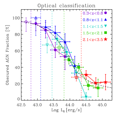
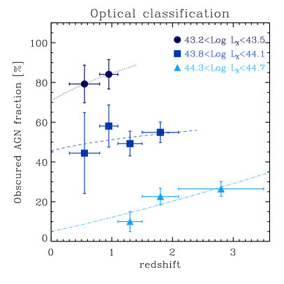
Figure 8: Left Panel: The fraction of optically obscured AGN is plotted versus the X-ray luminosity for different redshift bins (purple circles: $0.3\leq z<0.8$; blue upwards triangles: $0.8\leq z<1.1$; cyan downwards triangles: $1.1\leq z<1.5$; green squares: $1.5\leq z<2.1$ and red stars: $2.1\leq z<3.5$). The vertical dashed lines mark the luminosities above which the samples are complete in each redshift bin (of corresponding color). Empty symbols are from incomplete bins. The dashed line is the best fit to the entire data set across the whole redshift range. Right Panel: Redshift evolution of the fraction of Obscured AGN in different luminosity bins (only those for which we are complete have been shown). The dotted, dashed, and dot-dashed lines show the best fit evolution in the three luminosity interval, respectively.

In Merloni et al. (2014) we have examined the luminosity and redshift dependence of the fraction of AGN classified as obscured, both optically and from the X-ray spectra. The sample, X-ray selected in the XMM-COSMOS field, was selected on the basis of the estimated rest frame 2-10 keV flux, in order to avoid as much as possible biases due to the $z-N_{\rm H}$ degeneracy for obscured AGN.

The left hand panel of Figure 8 shows such a fraction as a function of intrinsic X-ray luminosity in five different redshift bins. The decrease of the obscured AGN fraction with luminosity is strong, and confirms previous studies on the XMM-COSMOS AGN (Brusa et al., 2010). The dashed line, instead, shows the best fit relations to the optically obscured AGN fraction obtained combining all redshift bins.

One of the most important conclusions of the work of Merloni et al. (2014) was that for about 30% of all X-ray selected AGN the optical- and X-ray-based classifications into obscured and un-obscured sources disagree. For this reason, the left panel of Figure 9, which shows the fraction of (X-ray classified) obscured AGN as a function of intrinsic 2-10 keV X-ray luminosity ($L_{\rm X}$) is significantly different from that of Figure 8. In particular, at low luminosity about one third of the AGN have un-obscured X-ray spectra but no broad emission lines or prominent blue accretion disc continuum in their optical spectra, while, on the other hand, about 30% of the most luminous QSOs have obscured X-ray spectra despite showing clear broad emission line in the optical spectra.

We plot in the right panels of Figures 8 and 9 the fraction of obscured AGN as a function of redshift, for three separate luminosity intervals and for the optical and X-ray classifications, respectively. Only bins where the sample is complete are shown. For optically classified AGN, we do not see any clear redshift evolution, apart from the highest luminosity objects (i.e. genuine QSOs in the XMM-COSMOS sample, with $L_{\rm X}$ between 10^44.3 and 10^44.7 erg/s). To better quantify this, we have fitted separately the evolution of the obscured fraction in the three luminosity bins with the function: $F_{\rm obs}=B\times(1+z)^{\delta}$.

The best fit relations are shown as thin lines in the right panels of Figures 8 and 9. For the optical classification, as anticipated, we measure a significant evolution ($\delta_{\rm OPT}>0$) only for the most luminous objects, with $\delta_{\rm OPT}=1.27\pm 0.62$. For the X-ray classification, we observe a significant evolution with redshift both at the lowest and highest luminosities, where the fraction of X-ray obscured AGN increases with $z$, consistent with previous findings by numerous authors (La Franca et al., 2005; Treister & Urry, 2006; Hasinger, 2008; Fiore et al., 2012; Vito et al., 2013). A more robust assessment of the redshift evolution of the obscured AGN fraction, however, would require a more extensive coverage of the $L-z$ plane than that afforded by the flux-limited XMM-COSMOS sample.

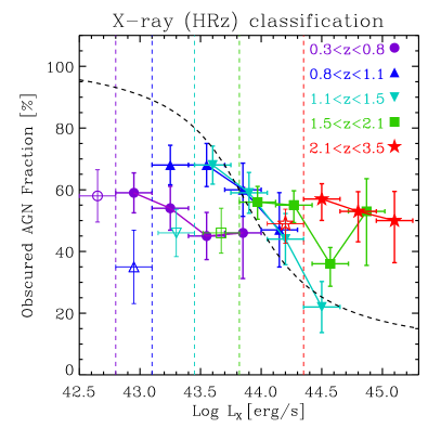
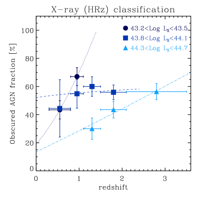
Figure 9: Left panle: The fraction of X-ray obscured AGN is plotted versus the X-ray luminosity for different redshift bins (purple circles: $0.3\leq z<0.8$; blue upwards triangles: $0.8\leq z<1.1$; cyan downwards triangles: $1.1\leq z<1.5$; green squares: $1.5\leq z<2.1$ and red stars: $2.1\leq z<3.5$). The vertical dashed lines mark the luminosities above which the samples are complete in each redshift bin (of corresponding color). Empty symbols are from incomplete bins. The dashed line is here plotted as a reference, and represent the best fit to the absorbed AGN fraction vs. luminosity relation for optically obscured AGN, from Fig. 8. Right Panel: Redshift evolution of the fraction of Obscured AGN in different luminosity bins (only those for which we are complete have been shown). The dotted, dashed, and dot-dashed lines show the best fit evolution in the three luminosity interval, respectively.

3.4 The SED of low luminosity AGN

Irrespective of where and when was most of the mass in SMBH accreted (and we will see in section 5 that this happened most likely at high accretion rates), the steepness of the AGN luminosity function tells us that most of the time in the life of a nuclear black hole is spent in a low accretion rate, low luminosity regime: the ubiquity of SMBH in the nuclei of nearby galaxies implies that, in the local Universe, AGN of low and very low luminosity vastly outnumber their bright and active counterparts. However, at lower accretion rates the precise determination of AGN SED is severely hampered by the contamination from stellar light (as we discussed in more detail in section 2), and very high resolution imaging is needed to identify the accretion-related emission. This is of course possible only for nearby galaxies, and only a limited number of reliable SED of LLAGN are currently known Ho (2008). An important step towards the classification of AGN in terms of their specific modes of accretion was taken by Merloni et al. (2003) and Falcke et al. (2004), whereby a “fundamental plane” relation between mass, X-ray and radio core luminosity of active black holes was discovered and characterized in terms of accretion flows. In particular, the observed scaling between radio luminosity, X-ray luminosity and BH mass implies that the output of low-luminosity AGN is dominated by kinetic energy rather than by radiation (Sams et al., 1996; Merloni & Heinz, 2007; Hardcastle et al., 2007; Best & Heckman, 2012). This is in agreement with the average SED of LLAGN (Ho, 2008; Nemmen et al., 2014) displaying a clear lack of thermal (BBB) emission associated to an optically thick accretion disc, strongly suggestive of a “truncated disc” scenario and of a radiative inefficient inner accretion flow (see Figure 10).

  

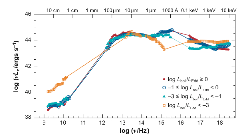
Figure 10: Energy spectra of a compilation of AGN at different Eddington-scaled luminosities (from Ho (2008)).

4 AGN luminosity functions and their evolution

The Luminosity Functions (LF) $\phi(L)$ describe the space density of sources of different luminosity $L$, so that $dN=\phi(L)dL$ is the number of sources per unit volume with luminosity in the range $L+dL$. In this section we review the current observational state of affairs in the study of AGN luminosity functions, in various parts of the electromagnetic spectrum (from radio to X-rays). Well constrained single-band luminosity functions, together with a good understanding of the AGN SED (and its evolution), can then be used to infer the “bolometric” LF, i.e. the full inventory of the radiative energy release onto accreting black holes.

4.1 The evolution of radio AGN

The observed number counts distribution of radio sources (see e.g. Merloni & Heinz, 2013) has been used for many years as a prime tool to infer properties of the cosmological evolution of radio AGN, mainly because of the sensitivity of radio telescope to distant quasar, and of the difficulty in getting reliable counterpart identification and redshift estimate for large number of radio sources.

At bright fluxes, counts rise more steeply than the Euclidean slope $S^{-3/2}$. This was already discovered by the first radio surveys at meter wavelengths (Ryle & Scheuer, 1955), lending strong support for evolutionary cosmological models, as opposed to theories of a steady state universe.

At fluxes fainter than about a Jansky (or $\approx 10^{-14}$ ergs s^-1 cm^-2 at 1 GHz) the counts increase less steeply than $S^{-3/2}$, being dominated by sources at high redshift, thus probing a substantial volume of the observable universe.

At flux densities above a mJy the population of radio sources is largely composed by AGN. For these sources, the observed radio emission includes the classical extended jet and double lobe radio sources as well as compact radio components more directly associated with the energy generation and collimation near the central engine.

The deepest radio surveys, however, (see e.g. Padovani et al. 2009 and references therein), probing well into the sub-mJy regime, clearly show a further steepening of the counts. The nature of this change is not completely understood yet, but in general it is attributed to the emergence of a new class of radio sources, most likely that of star-forming galaxies and/or radio quiet AGN (see Fig. 11). Unambiguous solutions of the population constituents at those faint flux levels requires not only identification of the (optical/IR) counterparts of such faint radio sources, but also a robust understanding of the physical mechanisms responsible for the observed emission both at radio and optical/IR wavelengths.

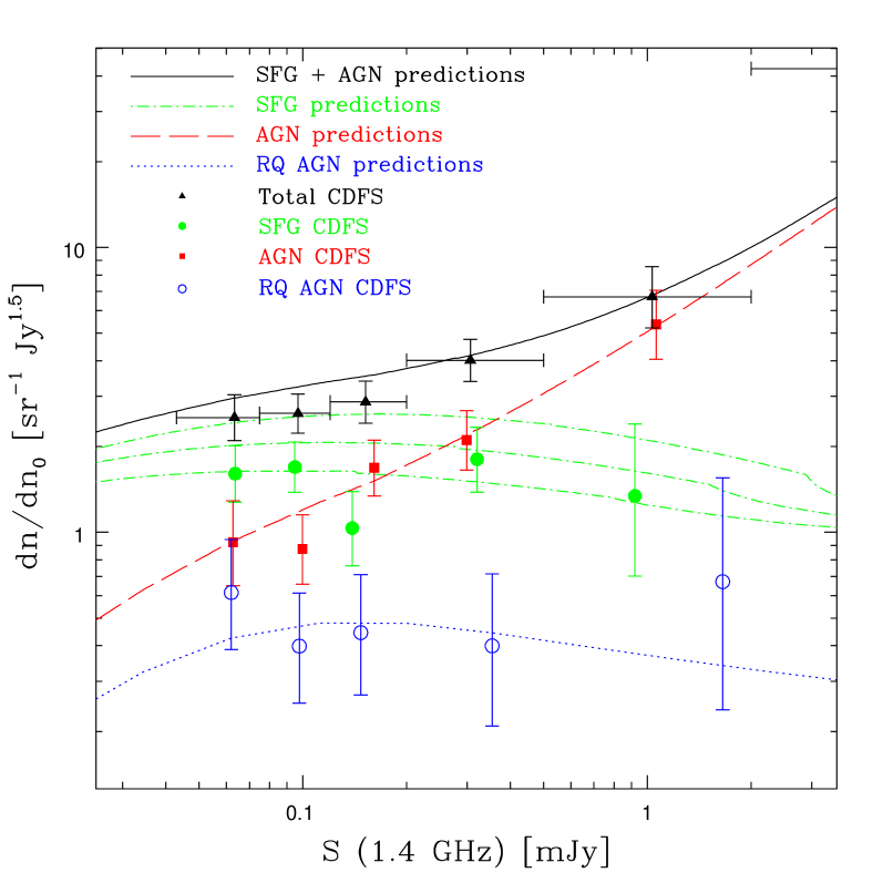
Figure 11: Euclidean normalized 1.4 GHz CDFS radio source counts: total counts (black triangles), Star Forming Galaxies (filled green circles), all AGNs (red squares), and radio- quiet AGNs (open blue circles). Error bars correspond to 1$\sigma$ errors. Model calculations refer to SFG (green dotted–dashed lines), displayed with a 1$\sigma$ range on the evolutionary parameters, all AGNs (red dashed line), radio-quiet AGNs (blue dotted line), and the sum of the first two (black solid line). From Padovani et al. (2009).

Thus, the complex shape of the observed number counts provides clues about the evolution of radio AGN, as well as on their physical nature, even before undertaking the daunting task of identifying substantial fractions of the observed sources, determining their distances, and translating the observed density of sources in the redshift-luminosity plane into a (evolving) luminosity function. Pioneering work from Longair (1966) already demonstrated that, in order to reproduce the narrowness of the observed ’bump’ in the normalized counts around $1$ Jy, only the most luminous sources could evolve strongly with redshift. This was probably the first direct hint of the intimate nature of the differential evolution AGN undergo over cosmological times.

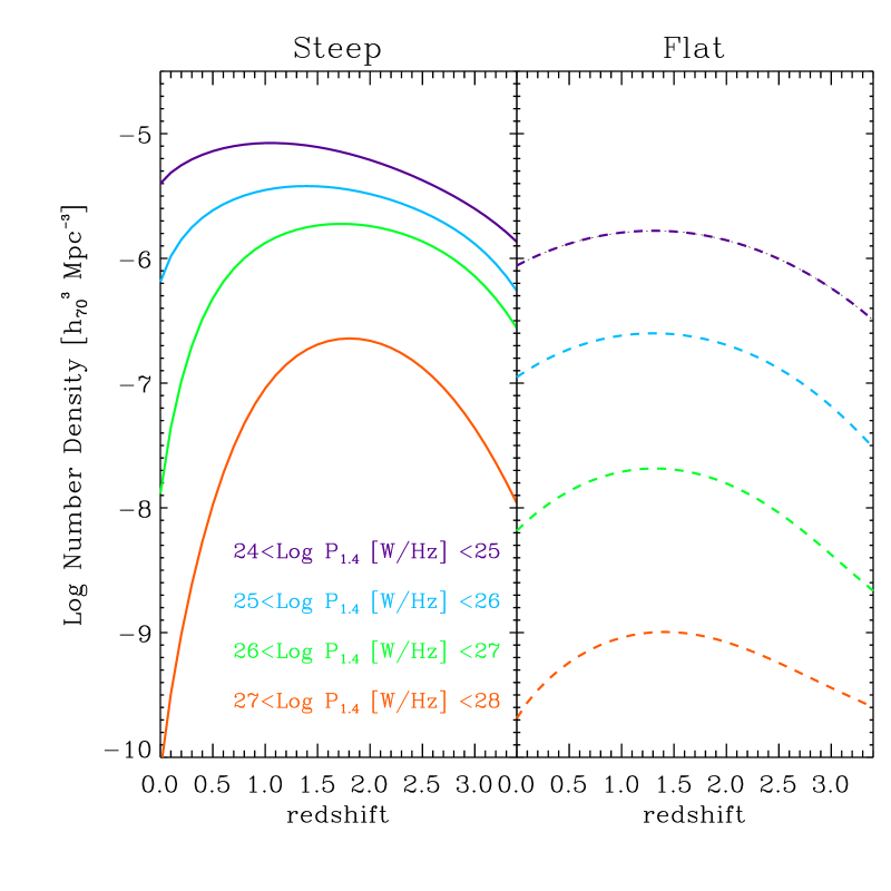
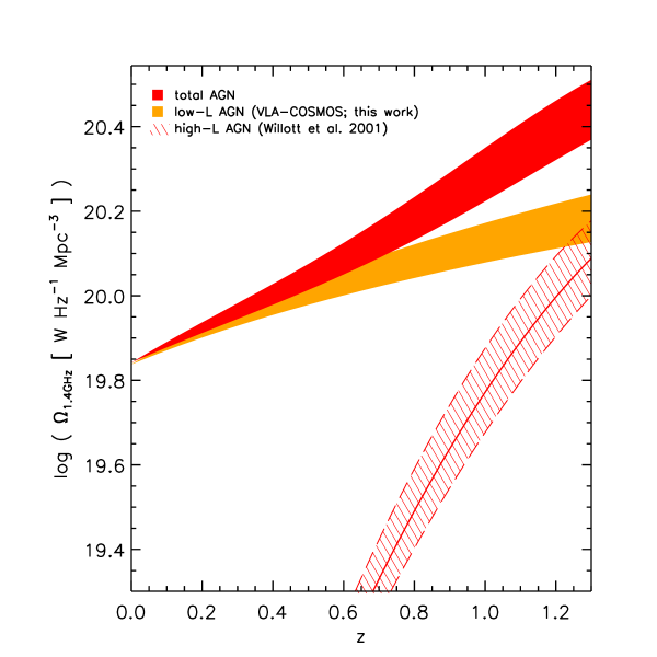
Figure 12: The radio view of AGN downsizing. Left: Best fit number density evolution of radio sources of different power, taken from the models of Massardi et al. (2010), for steep and flat spectrum sources in the left and right panels, respectively. Right: Evolution of the comoving 20 cm integrated luminosity density for VLA-COSMOS AGN (orange curve) galaxies for $z<1.3$. Also shown is the evolution of the high-luminosity radio AGN, adopted from (Willott et al. 2001, hatched region; the thick and dashed lines correspond to the mean, maximum and minimum results, respectively). The evolution for the total AGN population, obtained by co-adding the VLA-COSMOS and high luminosity AGN energy densities, is shown as the red-shaded curve (adopted from Smolčić et al. 2009).

Indeed, many early investigations of high redshift radio luminosity functions (see, e.g., Danese et al. 1987) demonstrated that no simple LF evolution models could explain the observed evolution of radio sources, with more powerful sources (often of FRII morphology) displaying a far more dramatic rise in their number densities with increasing redshift (see also Willott et al. 2001).

Trying to assess the nature of radio AGN evolution across larger redshift ranges requires a careful evaluation of radio spectral properties of AGN. Steeper synchrotron spectra are produced in the extended lobes of radio jets, while flat spectra are usually associated with compact cores. For objects at distances such that no radio morphological information is available, the combination of observing frequency, K-corrections, intrinsic source variability and orientation of the jet with respect to the line of sight may all contribute to severe biases in the determination of the co-moving number densities of sources, especially at high redshift (Wall et al., 2005).

In a very extensive and equally influential work Dunlop & Peacock (1990) studied the evolution of the luminosity functions of steep and flat spectrum sources separately. They showed that the overall redshift evolution of the two classes of sources were similar, with steep spectrum sources outnumbering flat ones by almost a factor of ten. Uncertainties remained regarding the possibility of a high-redshift decline of radio AGN number densities. The issue is still under discussion, with the most clear evidence for such a decline observed for flat-spectrum radio QSO at $z>3$ (Wall et al., 2005), consistent with the most recent findings of optical and X-ray surveys.

Under the simplifying assumption that the overall radio AGN population can be sub-divided into steep and flat spectrum sources, characterized by a power-law synchrotron spectrum $S_{\nu}\propto\nu^{-\alpha}$, with slope $\alpha_{\rm flat}=0.1$ and $\alpha_{\rm steep}=0.8$, respectively, a redshift dependent luminosity function can be derived for the two populations separately, by fitting simple models to a very large and comprehensive set of data on multi-frequency source counts and redshift distributions obtained by radio surveys at $\nu<5$ GHz (Massardi et al., 2010). The comoving number densities in bins of increasing radio power (at 1.4 GHz) from the resulting best fit luminosity function models are shown in the left panel of Figure 12.

Radio AGN, both with steep and flat spectrum, show the distinctive feature of a differential density evolution, with the most powerful objects evolving more strongly towards higher redshift, a phenomenological trend that, in the current cosmologist jargon, is called “downsizing”.

Recent radio observational campaigns of large multi-wavelength sky surveys have also corroborated this view, by providing a much more detailed picture of low luminosity radio AGN. For example, the work of Smolčić et al. (2009) on the COSMOS field showed that radio galaxies with $L_{\rm 1.4GHz}<few\times 10^{25}\,{\rm WHz^{-1}}$ evolve up to $z\simeq 1$, but much more mildly than their more luminous counterparts, as shown in the right panel Figure 12.

In the local Universe, the combination of the SDSS optical spectroscopic survey with the wide-area, moderately deep VLA surveys (NVSS, Condon et al. 1998 and FIRST, Becker et al. 1995), have been used by Best & Heckman (2012) to gain a powerful insight on the radio AGN population. They found not only that the radio AGN population can be clearly distinct into two sub-groups on the basis of their optical emission line properties (high- and low-excitations radio galaxies, HERG and LERG, respectively), but that dichotomy corresponds to a more profound difference in the accretion mode onto their respective black holes: HERG typically have accretion rates between one per cent and 10 per cent of their Eddington rate, and appear to be in a radiative efficient mode of accretion, while most LERG accrete with an Eddington ratio of less than one per cent. In addition, the two populations show differential cosmic evolution at fixed radio luminosity: HERG evolve strongly at all radio luminosities, while LERG show weak or no evolution, consistent with the general trends observed in the more distant Universe, and described above.

4.2 Optical and Infrared studies of QSOs

Finding efficient ways to select QSO in large optical surveys, trying to minimize contamination from stars, white dwarfs and brown dwarfs has been a primary goal of optical astronomers since the realization that QSO were extragalactic objects often lying at cosmological distances (Schmidt & Green, 1983; Richards et al., 2006).

Optical surveys remain an extremely powerful tool to uncover the evolution of un-obscured QSOs up to the highest redshift ($z\sim 6$). In terms of sheer numbers, the known population of SMBH is dominated by such optically selected AGN (e.g. more that $3\times 10^{5}$ QSOs have been identified in the first three generations of the Sloan Digital Sky Survey, Pâris et al. 2014), essentially due to the yet unsurpassed capability of ground-based optical telescopes to perform wide-field, deep surveys of the extra-galactic sky.

As for the general evolution of the optically selected QSO luminosity function, it has been known for a long time that luminous QSOs were much more common at high redshift ($z\sim 2$). Nevertheless, it is only with the aid of the aforementioned large and deep surveys covering a wide enough area of the distance-luminosity plane that it was possible to put sensible constraints on the character of the observed evolution. Most recent attempts Croom et al. (2009) have shown unambiguously that optically selected AGN do not evolve according to a simple pure luminosity evolution, but instead more luminous objects peaked in their number densities at redshifts higher than lower luminosity objects, as shown in the left panel of Figure 13.

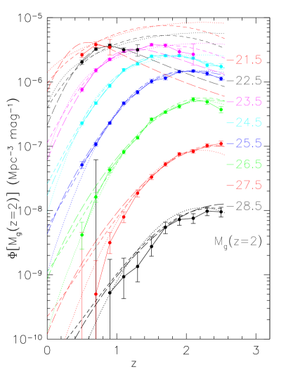
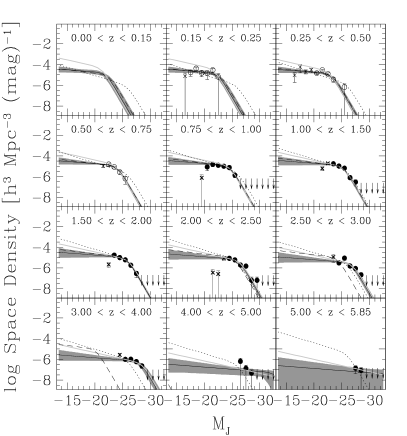
Figure 13: Left: The combined 2SLAQ and SDSS optical QSO luminosity function plotted as a function of redshift for different absolute $g$ band magnitude intervals (the brightest at the bottom of the plot and the faintest at the top). The measured LF is compared to the best fit PLE model (Pure Luminosity Evolution, dotted lines), smooth LDDE model (Luminosity Dependent Density Evolution, long dashed lines) and LADE (Luminosity And Density Evolution) model (short dashed lines). From Croom et al. (2009); Right: J-band luminosity function of mid-IR-selected AGN for several redshift bins. The crosses show points that were not used in the fits. The best-fit LADE, PLE, and pure PDE models are shown by the solid, dashed, and dotted line, respectively, although only the LADE model is an acceptable fit to the data. The shaded area shows the 2$\sigma$ confidence region for the LADE fit. For reference, the solid light gray line shows the best-fit LADE model to a sample from a combined IR/X-ray selection. From Assef et al. (2011).

As I discussed in section 3.3, according to the AGN unification paradigm obscuration comes from optically thick dust blocking the central engine along some lines of sight. The temperature in this structure, which can range up to 1000K (the typical dust sublimation temperature), and the roughly isotropic emission toward longer wavelengths should make both obscured and un-obscured AGNs very bright in the mid- to far-infrared bands. This spectral shift of absorbed light to the IR has allowed sensitive mid-infrared observatories (IRAS, ISO, Spitzer) to deliver large numbers of AGN (see, e.g. Treister et al., 2006).

Deep surveys with extensive multi-wavelength coverage have been used to track the evolution of active galaxies in the mid-infrared (see, e.g. Assef et al., 2011; Delvecchio et al., 2014). Strengthening similar conclusions discussed above from other wavelengths, IR-selected AGN do not appear to evolve following either a ’pure luminosity evolution’ or ’pure density evolution’ parametrizations, but require significant differences in the evolution of bright and faint sources, with the number density of the former declining more steeply with decreasing redshift than that of the latter (see the right panel in Figure 13).

The problem with IR studies of AGN evolution, however, lies neither in the efficiency with which growing supermassive black holes can be found, nor with the completeness of the AGN selection, which is clearly high and (almost) independent of nuclear obscuration, but rather in the very high level of contamination, as we discussed in section 2. IR counts are, in fact, dominated by star forming galaxies at all fluxes: unlike the case of the CXRB, AGN contribute only a small fraction (up to 2-10%) of the cosmic IR background radiation (Treister et al., 2006), and similar fractions are estimated for the contribution of AGN at the “knee” of the total IR luminosity function at all redshifts. This fact, and the lack of clear spectral signatures in the nuclear, AGN-powered emission in this band, implies that secure identification of AGN in any IR-selected catalog often necessitates additional information from other wavelengths, usually radio, X-rays, or optical spectroscopy.

In the best cases (such as the COSMOS and CDFS fields), accurate SED modelling of IR selected galaxies can be used to identify reliably AGN (at least those accreting at a substantial rate). Delvecchio et al. (2014) have indeed been able to use a Herschel selected sample to derive the AGN luminosity function across a wide redshift range ($0<z<3$). Figure 14 shows the total integrated black hole accretion rate density derived from this work.

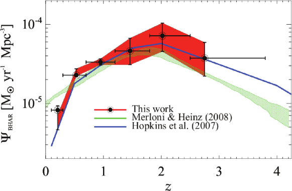
Figure 14: Black Hole Accretion Rate Density estimate from the Herschel selected AGN luminosity function, as a function of redshift (black circles). The red shaded area shows the $1\sigma$ uncertainty region. Previous estimates from different selection wavelengths (from Merloni & Heinz 2008, and Hopkins et al. 2007) are reported for comparison. From Delvecchio et al. (2014).

4.3 X-ray surveys

Due to the relative weakness of X-ray emission from stars and stellar remnants (magnetically active stars, cataclysmic variables and, more importantly, X-ray binaries are the main stellar X-ray sources), the X-ray sky is almost completely dominated by the evolving SMBH population, at least down to the faintest fluxes probed by current X-ray focusing telescopes (see eq. (3)).

In particular, the Cosmic X-ray Background (CXRB) radiation can be considered as the ultimate inventory of the energy released by the process of accretion onto black holes throughout the history of the Universe. Detailed modelling of the CXRB over the years, so-called “synthesis models” of the CXRB (Gilli et al., 2007; Treister et al., 2009), evolved in parallel with our deeper understanding of the physical properties of accreting black holes, and of their cosmological evolution. Today, deep extragalactic surveys with X-ray focusing telescopes, mainly Chandra and XMM-Newton, have resolved about $\sim 80-90\%$ of the CXRB. These observations have shown unambiguously that a similar fraction of the CXRB emission is produced by the emission of supermassive black holes in AGN at cosmological distances (see Figure 15).

The goal of reaching a complete census of evolving AGN, and thus of the accretion power released by SMBH in the history of the universe has therefore been intertwined with that of fully resolving the CXRB into individual sources. Accurate determinations of the CXRB intensity and spectral shape, coupled with the resolution of this radiation into individual sources, allow very sensitive tests of how the AGN luminosity and obscuration evolve with redshift.

The most recent CXRB synthesis models have progressively reduced the uncertainties in the absorbing column density distribution. When combined with the observed X-ray luminosity functions, they provide an almost complete census of the Compton-thin AGN (i.e., those obscured by columns $N_{\rm H}<\sigma_{\rm T}^{-1}\simeq 1.5\times 10^{24}$ cm^-2, where $\sigma_{\rm T}$ is the Thomson cross section). This class of objects dominates the counts in the lower energy X-ray energy band, where almost the entire CXRB radiation has been resolved into individual sources Worsley et al. (2005).

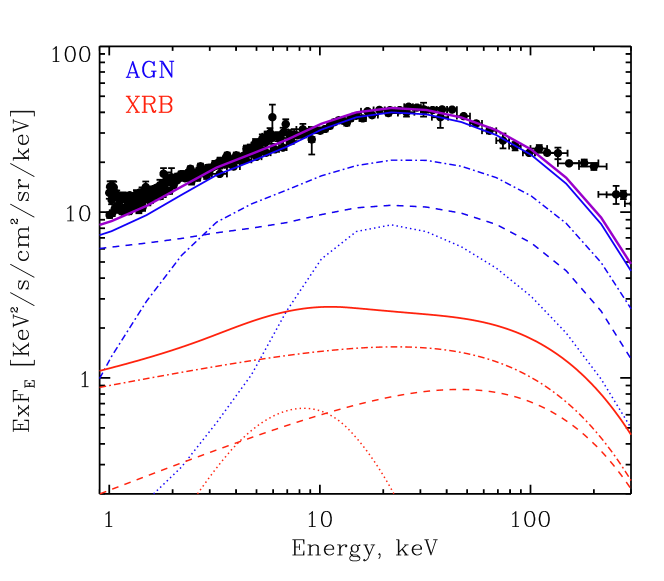
Figure 15: Contribution of supermassive black holes in AGN and stellar mass black holes in X-ray binaries to the spectral intensity of the Cosmic X-ray background. Points with error bars show the observed CXRB brightness (as compiled from Gilli et al. (2007)). The blue solid line is the overall contribution of AGN, which is the sum of the contributions from: i) un-obscured AGN (i.e. those with absorbing column density $N_{\rm H}<10^{22}$ cm², dashed blue line); ii) obscured, Compton-Thin AGN (with $10^{22}<N_{\rm H}<10^{24}$ cm², dot-dashed blue line) and iii) heavily obscured, Compton-Thick sources ($N_{\rm H}>10^{24}$ cm², dotted blue line). The computation is based on the Gilli et al. (2007) synthesis model. The red solid line is the integrated contribution of high-mass X-ray binaries in star-forming galaxies, computed as described in Dijkstra et al. (2012). It is further subdivided into: i) Ultra-Luminous X-ray sources (Ultra-luminous X-ray sources, ULX, dot-dashed red line); ii) black hole High-mass X-ray binaries (dashed red line) and iii) accreting neutron stars and pulsars (dotted red line). Because of the shallow slope of the X-ray luminosity function of compact X-ray sources in star-forming galaxies, X-ray emission of the latter is dominated by the most luminous sources – stellar mass black holes accreting matter from the massive companion star. Adapted from Gilfanov & Merloni (2014).

Synthesis models of the X-ray background, like the one shown in Figure 15 ascribe a substantial fraction of this unresolved emission to heavily obscured (Compton-thick) AGN. However, because of their faintness even at hard X-ray energies, their redshift and luminosity distribution is very hard to determine, and even their absolute contribution to the overall CXRB sensitively depends on the quite uncertain normalization of the unresolved emission at hard X-ray energies. Overall the CXRB is relatively insensitive to the precise Compton-thick AGN fraction (Akylas et al., 2012). The quest for the physical characterization of this “missing” AGN population, most likely dominated by Compton thick AGN, represents one of the last current frontiers of the study of AGN evolution at X-ray wavelengths.

However, Compton Thick AGN still leaves characteristics imprints in the shape of AGN X-ray spectra, so that the deepest X-ray surveys, along with extensive multi-wavelength coverage of X-ray survey regions, have allowed the identification significant samples of Compton-thick AGN at moderate to high redshifts (Brightman & Nandra, 2012; Georgantopoulos et al., 2013; Buchner et al., 2014; Brightman et al., 2014).

Recently, Buchner et al. (2015) developed a novel non-parametric method for determining the space density of AGN as a function of accretion luminosity, redshift and hydrogen column density, building on the X-ray spectral analysis of Buchner et al. (2014). Applying their Bayesian spectral analysis technique of a realistic, physically motivated model to a multi-layered survey determine the luminosity and level of obscuration in a large sample of X-ray selected AGN across a wide range of redshifts.

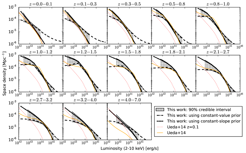
Figure 16: Total X-ray luminosity function in the 2-10 keV spectral band. Each panel corresponds to a different redshift interval. Dashed and solid black lines represent the results obtained with two different generic choices of priors for the non-parametric description of the data; the difference in the reconstructions between the two is therefore an indication of whether the data or the priors dominate the result. The hatched regions indicate a measure of the uncertainty, using the 10%-90% quartiles of the posterior samples from both priors together. The orange thin solid line shows the reconstruction by Ueda et al. (2014). The dotted red curve is their local ($z=0.1$) luminosity function kept constant across all panels for comparison. From Buchner et al. (2015)

.

Figure 16 shows the total (i.e. including Compton-thick objects) X-ray luminosity function (XLF) in the 2-10 keV spectral band, together with a comparison with a recent comprehensive study of the XLF by Ueda et al. (2014). The overall shape of the luminosity function is a double power-law with a break or bend at a characteristic luminosity, $L*$, the value of which increases with redshift. As found in previous studies, the space density shows a rapid evolution up to around $z\approx 1$ at all luminosities, being most prominent at high luminosities due to the positive evolution of $L*$.

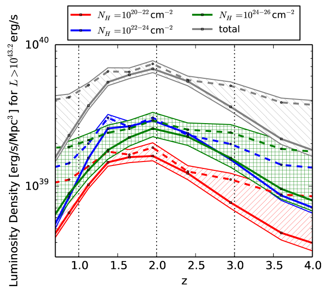
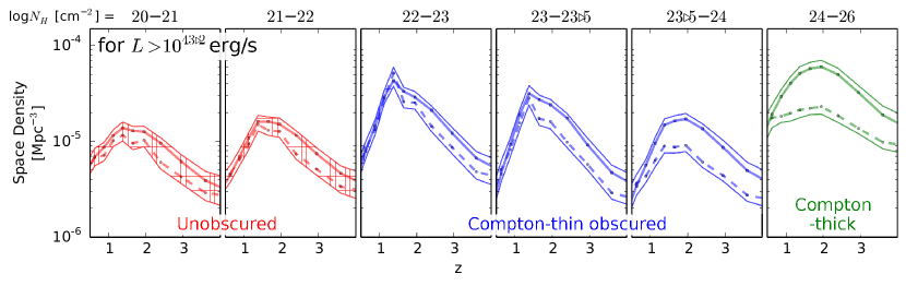
Figure 17: Top panel: Evolution of the X-ray luminosity density of AGN with $L_{\rm X}>10^{43.2}$ erg/s, for various column densities. The luminosity output of AGN experiences a rise and fall in density in the $z=1--3.5$ range (total as top gray shaded region). The strongest contribution to the luminosity density is due to obscured, Compton-thin (blue shaded region) and Compton-thick AGN (green shaded region), which contribute in equal parts to the luminosity. The emission from un-obscured AGN (red shaded region, bottom) is significantly smaller. Bottom panel: Redshift evolution of space density of AGN split by the level of obscuration. Different panels correspond to different hydrogen column density interval as indicated at the top. From Buchner et al. (2015).

Figure 17 shows the derived luminosity density (in erg/s/Mpc^-3) for X-ray emitting AGN, split into un-obscured ones, Compton-thin and -thick sources. Buchner et al. (2015) found that about 75% of the AGN space density, averaged over redshift, corresponds to sources with column densities $N_{\rm H}>10^{22}$ cm^-2. The contribution of obscured AGN to the accretion density of the Universe over cosmic time is similarly large ($\approx 75$%). The contribution to the luminosity density by Compton-thick AGN is $39\pm 6$%. Crucially, for the first time the uncertainty on what used to be called “missing” AGN population is below 10%, and the Compton-thick AGN fraction appears consistent with the requirement of CXRB synthesis models, suggesting we are approaching a reliable, comprehensive census of accretion onto Supermassive black hole over a large fraction of the age of the Universe.

4.4 Bolometric AGN luminosity functions and the history of accretion

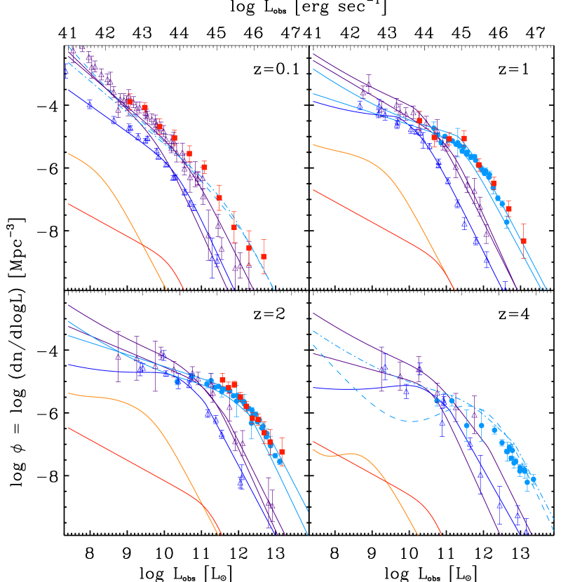
Figure 18: A compilation of luminosity functions observed in various energy bands. The logarithm of the number of AGN per unit comoving volume and unit logarithm of luminosity is plotted as a function of the observed luminosity (in solar units). Observational points for IR (15$\mu$m; filled red squares), B-band (filled blue circles), soft- (0.5-2 keV; empty blue triangles) and hard-X-rays (2-10 keV; empty purple triangles) are shown alongside published analytic fits for each band (solid lines in corresponding colors). The best-fit radio luminosity functions of steep- and flat-spectrum radio sources from Massardi et al. (2010) are also shown for comparison, with orange and red thick lines, respectively. The observed mismatch among the various luminosity functions in Fig. 18 is due to a combination of different bolometric corrections and incompleteness due to obscuration. Courtesy of P. Hopkins

As we have seen in the previous sections, a qualitatively consistent picture of the main features of AGN evolution is emerging from the largest surveys of the sky in various energy bands. Strong (positive) redshift evolution of the overall number density, as well as some differential evolution (with more luminous sources being more dominant at higher redshift) characterize the evolution of AGN (see Figure 18).

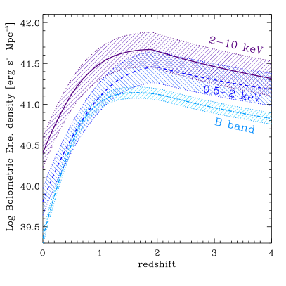
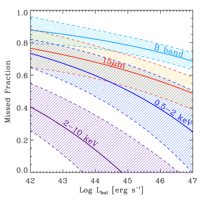
Figure 19: Left: The redshift evolution of the bolometric energy density for AGN selected in different bands. Bolometric corrections from Hopkins et al. (2007) have been used, and the shaded areas represent the uncertainty coming from the bolometric corrections only. Right: The fraction of AGN missed by observations in any specific band as a function of the intrinsic bolometric luminosity of the AGN. Red, light blue, dark blue and purple shaded areas correspond to rest-frame mid-IR (15$\mu$m), UV (B-band), soft X-rays (0.5-2 keV) and hard X-rays (2-10 keV), respectively. The uncertainty on the missed fractions depend on the uncertainties of the bolometric corrections and on the shape of the observed luminosity functions only.

A thorough and detailed understanding of the AGN SED as a function of luminosity could in principle allow us to compare and cross-correlate the information on the AGN evolution gathered in different bands. A luminosity dependent bolometric correction is required in order to match type I (unabsorbed) AGN luminosity functions obtained by selecting objects in different bands. This is, in a nutshell, a direct consequence of the observed trend of the relative contribution of optical and X-ray emission to the overall SED (the $\alpha_{\rm ox}$ parameter) as a function of luminosity (see the left panel of Fig. 7).

Adopting a general form of luminosity-dependent bolometric correction, and with a relatively simple parametrization of the effect of the obscuration bias on the observed LF, Hopkins et al. (2007) were able to project the different observed luminosity functions in various bands into a single bolometric one, $\phi(L_{\rm bol})$. As a corollary from such an exercise, we can then provide a simple figure of merit for AGN selection in various bands by measuring the bolometric energy density associated with AGN selected in that particular band as a function of redshift. I show this in the left panel of Figure 19 for four specific bands (hard X-rays, soft X-rays, UV, and mid-IR). From this, it is obvious that the reduced incidence of absorption in the 2-10 keV band makes the hard X-ray surveys recover a higher fraction of the accretion power generated in the universe than any other method.

While optical QSO surveys miss more than three quarters of all AGN of any given $L_{\rm bol}$, hard X-ray selection only fails to account for about one third of all AGN, the most heavily obscured (Compton-thick) ones, as shown in the right panel of Figure 19. It is important to note that the high missed fraction for mid-IR selected AGN is a direct consequence of the need for (usually optical) AGN identification of the IR sources, so that optically obscured active nuclei are by and large missing in the IR AGN luminosity functions considered here.

5 The Soltan argument: the Efficiency of Accretion

A reliable census of the bolometric energy output of growing supermassive black holes allows a more direct estimate of the global rate of mass assembly in AGN, and an interesting comparison with that of stars in galaxies. Together with the tighter constraints on the “relic” SMBH mass density in the local universe, $\rho_{\rm BH,0}$, provided by careful application of the scaling relations between black hole masses and host spheroids, this enables meaningful tests of the classical ’Soltan argument’ (Soltan, 1982), according to which the local mass budget of black holes in galactic nuclei should be accounted for by integrating the overall energy density released by AGN, with an appropriate mass-to-energy conversion efficiency.

Many authors have carried out such a calculation, either using the CXRB as a “bolometer” to derive the total energy density released by the accretion process (Fabian & Iwasawa, 1999), or by considering evolving AGN luminosity functions (Yu & Tremaine, 2002; Marconi et al., 2004; Merloni & Heinz, 2008). Despite some tension among the published results that can be traced back to the particular choice of AGN LF and/or scaling relation assumed to derive the local mass density, it is fair to say that this approach represents a major success of the standard paradigm of accreting black holes as AGN power-sources, as the radiative efficiencies needed to explain the relic population are within the range $\approx 0.06\div 0.40$, predicted by standard accretion disc theory Shakura & Sunyaev (1973).

In general, we can summarize our current estimate of the (mass-weighted) average radiative efficiency, $\langle\epsilon_{\rm rad}\rangle$, together with all the systematics uncertainties, within one formula, relating $\langle\epsilon_{\rm rad}\rangle$ to various sources of systematic errors in the determination of supermassive black hole mass density. From the integrated bolometric luminosity function, we get:

$$\frac{\langle\epsilon_{\rm rad}\rangle}{1-\langle\epsilon_{\rm rad}\rangle}\approx 0.075\left[\xi_{0}(1-\xi_{i}-\xi_{\rm CT}+\xi_{\rm lost})\right]^{-1}$$ (5)

where $\xi_{0}=\rho_{\rm BH,z=0}/4.2\times 10^{5}M_{\odot}{\rm Mpc}^{-3}$ is the local ($z=0$) SMBH mass density in units of 4.2$\times 10^{5}M_{\odot}{\rm Mpc}^{-3}$ Marconi et al. (2004); $\xi_{i}$ is the mass density of black holes at the highest redshift probed by the bolometric luminosity function, $z\approx 6$, in units of the local one, and encapsulate our uncertainty on the process of BH formation and seeding in proto-galactic nuclei (see e.g. Volonteri, 2010); $\xi_{\rm CT}$ is the fraction of SMBH mass density (relative to the local one) grown in heavily obscured, Compton Thick AGN; finally, $\xi_{\rm lost}$ is the fraction black hole mass contained in “wandering” objects, that have been ejected from a galaxy nucleus following, for example, a merging event and the subsequent production of gravitational wave, the net momentum of which could induce a kick capable of ejecting the black hole form the host galaxy.

The recent progresses on the tracking of heavily obscured AGN in deep X-ray surveys that we have highlighted in section 4.3 (Buchner et al., 2015) allows us to estimate the contributions of un-obscured AGN, Compton-thin and Compton-thick obscured AGN separately. Figure 20 shows an illustrative example of such a calculation, where, for the sake of simplicity, the X-ray radiative energy density evolutions of Buchner et al. (2015) have been used, assuming a constant bolometric correction and fixed the radiative efficiency of accretion to 10%. According to this computation, the fraction of black hole mass accreted in heavily obscured (CT) phases is $\xi_{\rm CT}\approx$ 35% (see Fig. 17), with $\xi_{i}<4$% (at $z=4$).

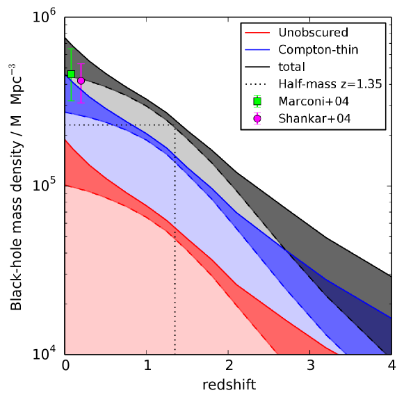
Figure 20: Redshift evolution of the total supermassive black holes mass density. The dark grey band shows the overall evolution, computed from the observed 2-10 keV luminosity function of Figure 16, assuming, for simplicity, a constant bolometric correction. The red band shows the un-obscured AGN contribution only, while the blue one is for Compton-thin objects, including un-obscured ones. Colored points with error bars represent estimates of the local SMBH mass density from Marconi et al. (2004) and Shankar et al. (2004). Courtesy of J. Buchner.

In the real evolution of SMBH, all the terms in eq. (5) must be linked at some level, as the radiative efficiency of accretion depends on the location of the innermost stable circular orbit, thus on the black hole spin, which itself evolves under the effects of both accretion and BH-BH mergers. Accurate models which keep track of both mass and spin evolution of SMBH could in principle be used, together with observational constraints from the AGN luminosity functions, to put constraints on those unknowns, providing a direct link between the relativistic theory of accretion and structure formation in the Universe (see e.g. Volonteri et al., 2013; Sesana et al., 2014). Pinning down the uncertainty of the luminosity density of accretion and of the bolometric corrections (properly including its dependence on black hole mass, accretion rate, possible redshift) will provide strong indirect bounds on the allowed population of seed and “wandering” black holes.

5.1 Quantifying the efficiency of kinetic energy release

We close this chapter with a brief discussion of the available estimates of the efficiency with which AGN are able to convert gravitational potential energy of the accreted matter into kinetic energy of the radio-emitting relativistic jets. This is a fundamental question for our understanding of accretion processes at low rates, with potentially crucial implication for the physical nature of feedback from AGN. To carry out this exercise, however, we need first to measure the total kinetic power carried by those jets.

The observed omni-presence of radio cores in low luminosity AGN and the observed increase in radio loudness of X-ray binaries at low luminosities can be placed on a solid theoretical footing. Jets launch in the innermost regions of accretion flows around black holes, and at low luminosities, these flows likely become mechanically (i.e., advectively) cooled.

Such flows can, to lowest order, be assumed to be scale invariant: a low luminosity accretion flow around a 10 solar mass black hole, accreting at a fixed, small fraction of the Eddington accretion rate, will be a simple, scaled down version of the same flow around a billion solar mass black hole (with the spatial and temporal scales shrunk by the mass ratio). It follows, then, that jet formation in such a flow should be similarly scale invariant.

This assumption is sufficient to derive a very generic relation between the radio luminosity emitted by such a scale invariant jet and the total (kinetic and electromagnetic) power carried down the jet, independent of the unknown details of how jets are launched and collimated (Heinz & Sunyaev, 2003): The synchrotron radio luminosity $L_{\nu}$ of a self-absorbed jet core depends on the jet power $P_{\rm jet}$ through

$$L_{\rm radio}\propto P_{\rm jet}^{\frac{17+8\alpha}{12}}M^{-\alpha}\sim P^{\frac{17}{12}}$$ (6)

where $M$ is the mass of the black hole and $\alpha\sim 0$ is the observable, typically flat radio spectral index of the synchrotron power-law emitted by the core of the jet. This relation is a result of the fact that the synchrotron photosphere (the location where the jet core radiates most of its energy) moves further out as the size scale and the pressure and field strength inside the jet increase (corresponding to an increase in jet power). As the size of the photosphere increases, so does the emission. The details of the power-law relationship are an expression of the properties of synchrotron emission.

For a given black hole, the jet power should depend on the accretion rate as $P_{\rm jet}\propto\dot{M}$ (this assumption is implicit in the assumed scale invariance). On the other hand, the emission from optically thin low luminosity accretion flows itself depends non-linearly on the accretion rate, roughly as $L_{\rm acc}\propto\dot{M}^{2}$, since two body processes like bremsstrahlung and inverse Compton scattering dominate, which depend on the square of the density. Thus, at low accretion rates, $L_{\rm radio}\sim L_{\rm bol}^{\frac{17}{24}}$, which implies that black holes should become more radio loud at lower luminosities (Heinz & Sunyaev, 2003; Merloni et al., 2003; Falcke et al., 2004). It also implies that more massive black holes should be relatively more radio loud than less massive ones, at the same relative accretion rate $\dot{M}/M$.

Equation 6 is a relation between the observable core radio flux and the underlying jet power. Once calibrated using a sample of radio sources with known jet powers, it can be used to estimate the jet power of other sources based on their radio properties alone (with appropriate provisions to account, statistically, for differences in Doppler boosting between different sources).

Nearby radio sources in massive clusters, where the cavities inflated by the relativistic jets can be used as calorimeters to estimate the total kinetic jet power (Allen et al., 2006; Rafferty et al., 2006; Merloni & Heinz, 2007; Cavagnolo et al., 2010) provide such a sample. Plotting the core (unresolved) radio power against the jet power inferred from cavity and shock analysis shows a clear non-linear relation between the two variables (Merloni & Heinz, 2007). Fitting this relation provides the required constant of proportionality and is consistent (within the uncertainties) with the power-law slope of $17/12$ predicted by eq. (6)

$$P_{\rm jet}=P_{0}\left(\frac{L_{\rm core}}{L_{0}}\right)^{\zeta}\sim 1.6\times 10^{36}\,{\rm ergs\,s^{-1}}\left(\frac{L_{\rm core}}{10^{30}\,{\rm ergs\,s^{-1}}}\right)^{0.81}$$ (7)

with an uncertainty in the slope $\zeta$ of 0.11, where $L_{\rm radio}=\nu L_{\nu}$ is measured at $\nu=5\,GHz$.

Because this relation was derived for the cores of jets, which display the characteristic flat self-absorbed synchrotron spectrum, care has to be taken when applying it to a sample of objects: only the core emission should be taken into account, while extended emission should be excluded. Moreover, the jet have relativistic bulk motions on the scales probed by the core emission, and the additional effect of relativistic beaming on the shape of the luminosity function has to be taken into account (Merloni & Heinz, 2007). As discussed in §4.1, radio luminosity functions are separated spectrally into flat and steep sources, and we can use both samples to limit the contribution of flat spectrum sources from both ends.

On the other hand, the same sample of radio AGN within clusters of galaxies with measured kinetic power can be used to derive the relationship between the extended, steep radio synchrotron luminosity and the jet power (Bîrzan et al., 2008; Cavagnolo et al., 2010). This has the advantage of being an isotropic luminosity indicator (i.e. unaffected by relativistic beaming, as in the case of the radio cores), but is also more sensitive to the environment (its density, magnetic field, kinematical state) the jet impinges upon. Indeed, the most recent analysis reveals a correlation between kinetic power and low-frequency (1.4 GHz) diffuse lobe emission of the form:

$$P_{\rm jet}\simeq 6.3\times 10^{36}\,{\rm ergs\,s^{-1}}\left(\frac{L_{\rm lobe}}{10^{30}\,{\rm ergs\,s^{-1}}}\right)^{0.7}$$ (8)

Given a radio luminosity function $\Phi_{\rm rad}$ (and, in the case of flat spectrum radio cores, an appropriate correction for relativistic boosting) eq. 7 and eq. 8 can be used to derive the kinetic luminosity function of jets (Heinz et al., 2007; Merloni & Heinz, 2008):

$$\Phi_{\rm kin}(P_{\rm jet})=\Phi_{\rm rad}\left[L_{0}\left(\frac{P_{\rm jet}}{P_{0}}\right)^{\frac{1}{\zeta}}\right]\frac{1}{\zeta}\frac{L_{0}}{P_{0}}\left(\frac{P_{\rm jet}}{P_{0}}\right)^{\frac{1-\zeta}{\zeta}}$$ (9)

The resulting kinetic luminosity functions (KLF) for the flat spectrum radio luminosity functions have been presented in Merloni & Heinz (2007). They showed that, at the low luminosity end, these KLF are roughly flat, implying that low luminosity source contributed a significant fraction of the total power. These are the low-luminosity AGN presumably responsible for radio mode feedback, and they dominate the total jet power output at low redshift.

One can also integrate the KLF and obtain the total kinetic energy density released by accreting black holes as radio-emitting relativistic jets. This is shown in the lower panel on the right hand side of Figure 21, both for flat spectrum radio cores (red curves, with different assumptions about the average bulk motion Lorentz factor of the jets, as labeled), and for the steep spectrum lobes (blue line), each with a nominal uncertainty derived from the scatter about the relations (7) and (8).

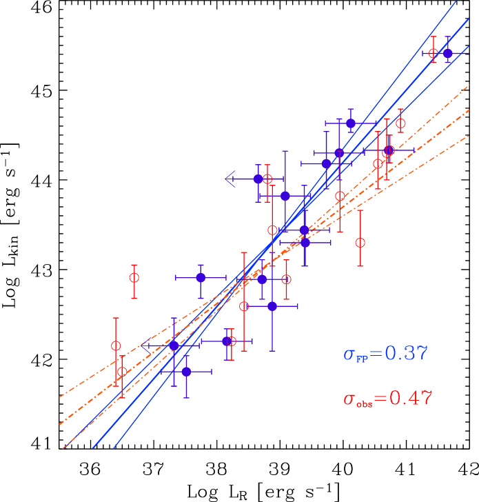
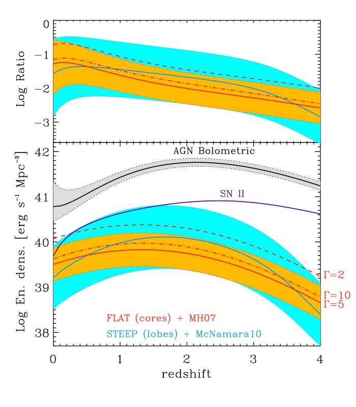
Figure 21: Left: Red open circles show jet power (measured from X-ray cavities) plotted against 5 GHz core radio luminosity (also shown in blue solid circles is a Doppler boosting corrected version of the same points) along the power-law fit given in eq. (7); adopted from Merloni & Heinz (2007). Right: The bottom panel shows the total kinetic energy density (in logarithmic scale) emitted by radio AGN. The red lines correspond to integrating the flat spectrum radio LF, using eq.(7) to obtain the jet power, with different lines marking the correction due to the assumed average bulk motion Lorentz factor, as labeled. The blue line corresponds to integrating the steep spectrum radio LF, using eq.(8) to obtain the jet power. Orange and cyan bands give an estimate of the uncertainty derived from the observed scatter in those relations. For comparison, the black line (with grey band) shows the bolometric radiative energy density from AGN, computed from Hopkins et al. (2007) bolometric LF, while the purple line is the estimated kinetic power injected into galaxies by core-collapse Supernovae. The top panel shows the evolution with redshift of the ratio between radiative and kinetic energy density released by growing black holes, separately for flat (red) and steep (blue) spectrum radio sources.

Integrating the luminosity function over $P_{\rm jet}$ gives the local jet power density $\rho_{\rm Pjet}$, which, at redshift zero, is of the order of $\langle\rho_{\rm Pjet}\rangle\sim 6\times 10^{39}\,{\rm ergs\,s^{-1}\,Mpc^{-3}}$, comparable to the local power density from supernovae, but will be significantly above the supernova power in early type galaxies (which harbor massive black holes prone to accrete in the radio mode but no young stars and thus no type 2 supernovae).

Finally, integrating $\Phi_{\rm kin}$ over redshift gives the total kinetic energy density $u_{\rm Pjet}$ released by jets over the history of the universe, $u_{\rm Pjet}\sim 3\times 10^{57}\,{\rm ergs\,Mpc^{-3}}$. By comparing this to the local black hole mass density $\rho_{\rm BH}$ we can derive the average conversion efficiency $\eta_{\rm jet}$ of accreted black hole mass to jet power: $\eta_{\rm jet}\equiv u_{\rm Pjet}/\rho_{\rm BH}c^{2}\approx 0.2\%-0.5\%$

In other words, about half a percent of the accreted black hole rest mass energy gets converted to jets, averaged over the growth history of the black hole.

For an average radiative efficiency of about $\langle\epsilon_{\rm rad}\rangle\approx 0.1$, as derived from the Soltan argument and discussed in the previous section, the mean kinetic-to-radiative power ratio of AGN is of the order of a few per cent, but possibly redshift dependent (see the top right panel of Fig. 21). However, since most black hole mass was accreted during the quasar epoch, when black holes were mostly radio quiet, about 90% of the mass of a given black hole was accreted at zero efficiency (assuming that only 10% of quasars are radio loud). Thus, the average jet production efficiency during radio loud accretion must be at least a factor of 10 higher, about 2%-5%, comparable to the radiative efficiency of quasars.