Quantum canonical ensemble: a projection operator approach

Abstract

Fixing the number of particles $N$, the quantum canonical ensemble imposes a constraint on the occupation numbers of single-particle states. The constraint particularly hampers the systematic calculation of the partition function and any relevant thermodynamic expectation value for arbitrary $N$ since, unlike the case of the grand-canonical ensemble, traces in the $N$-particle Hilbert space fail to factorize into simple traces over single-particle states. In this paper we introduce a projection operator that enables a constraint-free computation of the partition function and its derived quantities, at the price of an angular or contour integration. Being applicable to both bosonic and fermionic systems in arbitrary dimensions, the projection operator approach provides transparent integral representations for the partition function $Z_{N}$ and the Helmholtz free energy $F_{\!N}$ as well as for two- and four-point correlation functions. While appearing only as a secondary quantity in the present context, the chemical potential emerges as a by-product from the relation $\muup_{N}=F_{\!N+1}-F_{\!N}$, as illustrated for a two-dimensional fermion gas with $N$ ranging between 2 and 500.

1 Introduction

The calculation of the quantum mechanical partition function $Z_{N}$ of $N$ identical particles treated in the framework of the canonical ensemble remains a long-standing problem in many-body theory, even if the particles do not interact. The main difficulty hampering a systematic evaluation of $Z_{N}$ for moderate to large values of $N$ originates from the particle number constraint that is to be invoked explicitly. In order to overcome this problem, we introduce a projection operator in section 2 which is capable of dealing with the particle number constraint for non-interacting particles (bosons, fermions) as well as systems of interacting particles complying with particle number conservation. However, the formal applicability to interacting particles is hardly useful in practice, because the eigenstates and the eigenvalues of the energy for such systems are rarely available. Although modern particle physics surely treats strongly interacting particles, it faces the necessity of applying approximations which, in essence, apply a variety of transformation techniques that reduce the problem to treating ensembles of non-interacting particles. Thermal expectation values, based on statistical averages over ensembles of non-interacting particles, still provide the generic building blocks to set up perturbational and variational as well as other non-perturbative computation schemes. Essential ingredients for such approaches are the partition function and the two- and four-point correlation functions characterizing systems of non-interacting particles.

Keeping all this in mind, we believe it remains utterly relevant to consider a system of non-interacting particles and, therefore, we first examine its canonical partition function. As detailed in section 3, this results into a transparent integral representation for the partition function as well as the corresponding Helmholtz free energy and, hence, the chemical potential of $N$ non-interacting fermions or bosons. The integral representation also allows for a very simple derivation of a known recurrence relation for the partition function.

For $N$ harmonic oscillators in 1 dimension, the partition function could be obtained in closed form. The results are presented in section 4, for bosons as well as for fermions.

Section 5 contains a few numerical results related to the partition function and derived quantities of a finite size two-dimensional electron gas. Finally, the projection operator approach is applied once more in section 6 to derive generic expressions for the two- and four-point correlation functions. Some rather technical aspects are redirected to two appendices.

2 The canonical partition function: a projection operator approach

According to the nomenclature developed in the beginning of the 20th century, the statistical knowledge of a system in thermal equilibrium depends on the ensemble type: microcanonical, canonical or grand canonical. The canonical ensemble assumes that the exact number of particles in the system is known while its grand canonical counterpart merely requires that the average particle number be available. In theoretical studies of nuclear systems the number of particles is intrinsically dictated by the problem while for a great majority of solid-state systems only the average number of particles, in casu the density, is relevant.
However, recent technological developments in nanoelectronics made it possible to control the number of carriers in nanometer-scaled devices, making the actual number of particles a more important parameter than the average number or density. Hence it would be desirable to export and extend theoretical methods developed in nuclear physics to various many-body formalisms commonly used to treat nanometer-scaled solids. A typical many body approach often starts with a short investigation of the non-interacting system, usually formulated in terms of creation and annihilation operators. The use of these operators implicitly invokes a Fock space that, by construction, discards any reference to the number of particles whatsoever. However, if a description with a fixed number is mandatory, one needs to introduce a projection technique that limits the Fock space to a subspace that corresponds to a fixed number of particles, while still allowing for a formulation in terms of the second quantization operators. The projection technique used for nuclear models can accomplish this task and is found to operate also for the second quantization description of a many-body Hamiltonian. Correspondingly, the number of particles is fixed and emerges as a fixed eigenvalue of the number operator. After the projection one has to focus on the Fock subspace that is exclusively related to a fixed number of particles. In particular, the many-particle eigenfunctions of the projected Hamiltonian have to be calculated together with their energy spectrum and, afterwards, the probability density.

Motivated by the above observations, we consider a fixed number $N$ of of indistinguishable particles, fermions or bosons, described in the many-particle Fock space by a second-quantized Hamiltonian $\hat{\mathsf{H}}$. In order to preserve the number of particles, $\hat{\mathsf{H}}$ has to commute with the particle number operator $\hat{\mathsf{N}}$. Consequently, due to $[\hat{\mathsf{H}},\hat{\mathsf{N}}]=0$, many-particle eigenstates $|\psi_{j,N}\rangle$ of $\hat{\mathsf{H}}$ can be found that simultaneously diagonalize $\hat{\mathsf{H}}$ and $\hat{\mathsf{N}}$, i.e.

$$\hat{\mathsf{H}}|\psi_{j,N}\rangle=E_{\!j,N}|\psi_{j,N}\rangle,\qquad\hat{\mathsf{N}}|\psi_{j,N}\rangle=N|\psi_{j,N}\rangle,\qquad N=0,1,2,3,\ldots$$ (1)

Representing an arbitrary, allowable number of particles, the eigenvalues $N$ of $\hat{\mathsf{N}}$ are used to label the eigenstates $|\psi_{j,N}\rangle$ as well as the corresponding $E_{\!j,N}$. The index $j$ covers all remaining, internal quantum numbers that are labeling $E_{\!j,N}$ for a fixed value of $N$. For the sake of notational simplicity, we have omitted below any dependence on spin components which, however, can be incorporated into the formalism whenever required. Because $\hat{\mathsf{H}}$ operates in Fock space without any a priory reference to the number of particles, thermodynamics is usually expressed in the grand canonical ensemble (GCE). Within this framework, the chemical potential emerges as a Lagrange multiplier regulating the average number of particles, rather than imposing a sharply defined value of $N$, as required in the canonical ensemble (CE). In order to overcome this problem, we propose a projection operator that extracts a $N-$particle Hamiltonian $\hat{\mathsf{H}}_{N}$ out of $\hat{\mathsf{H}}$, while automatically invoking the canonical constraint of $N$ particles.

Let $\left\{\mathinner{\left|\psi_{n,M}\right\rangle}\right\}$ denote the complete set of eigenstates with an integer, nonnegative eigenvalue $M$ of the number operator $\hat{\mathsf{N}}\mathrm{:}$

$$\hat{\mathsf{N}}\mathinner{\left|\psi_{n,M}\right\rangle}=M\mathinner{\left|\psi_{n,M}\right\rangle},\quad\forall n,$$ (2)

and consider the operator

$$\hat{\mathsf{P}}_{\!N}=\frac{1}{2\pi}\int_{-\pi}^{\pi}\!\!\exp\left(\mathrm{i}(\hat{\mathsf{N}}-N)\theta\right)\mathrm{d}\theta,$$ (3)

with the obvious properties $\hat{\mathsf{P}}_{N}^{\dagger}=\hat{\mathsf{P}}_{\!N}$ and $\hat{\mathsf{P}}_{N}^{2}=\hat{\mathsf{P}}_{\!N}$. One furthermore observes that

$$\hat{\mathsf{P}}_{\!N}\mathinner{\left|\psi_{n,M}\right\rangle}=\frac{1}{2\pi}\int_{-\pi}^{\pi}\!\!\exp\left(\mathrm{i}(M-N)\theta\right)\mathrm{d}\theta\mathinner{\left|\psi_{n,M}\right\rangle}=\delta_{N,M}\mathinner{\left|\psi_{n,N}\right\rangle}$$ (4)

and hence

$$\hat{\mathsf{P}}_{\!N}\sum_{n,M}A_{n,M}\mathinner{\left|\psi_{n,M}\right\rangle}=A_{n,N}\mathinner{\left|\psi_{n,N}\right\rangle}.$$ (5)

Therefore, $\hat{\mathsf{P}}_{\!N}$ is a real projection operator which yields an eigenstate of the $N$-particle subspace if it acts on an arbitrary state of the entire many-particle Hilbert space. Consequently

$$\hat{\mathsf{H}}_{N}=\hat{\mathsf{P}}_{\!N}\hat{\mathsf{H}}\,\hat{\mathsf{P}}_{\!N}$$ (6)

is the $N$-particle Hamiltonian, extracted from the Hamiltonian $\hat{\mathsf{H}}$ in the many-particle Hilbert space. Note that the position representation of $\hat{\mathsf{H}}_{N}$ in principle coincides with the $N$-particle Hamiltonian of first quantization, as can be inferred from the algebraic treatment given in Ref. [1]. Although similar projection operators have been introduced before in statistical physics [2], nuclear and high-energy physics [3, 4, 5], we are not aware of its practical use as a particle number regulator in quantum statistics.

It is tempting to immediately suppose that the partition function for thermodynamical equilibrium is given by

$$Z_{N}(\beta)=\mathsf{Tr}\left(\mathrm{e}^{-\beta\hat{\mathsf{H}}_{N}}\right)$$ (7)

with some typical derived quantities as the Helmholtz free energy $F_{\!N}(\beta)$ and the internal energy $U_{\!N}(\beta)$, with $\beta=1/(k_{\mathrm{B}}T)$, where is the Boltzmann constant $(k_{\mathrm{B}}=1.3806568\times 10^{-23}\mathrm{J}\mathrm{K}^{-1})$ and $T$ the temperature in Kelvin:

$$F_{\!N}(\beta) =-\frac{1}{\beta}\ln\left(Z_{N}(\beta)\right)$$ (8)

$$U_{\!N}(\beta) =-\frac{\mathrm{d}}{\mathrm{d}\beta}\ln\left(Z_{N}(\beta)\right).$$ (9)

Although correct, these equation should be handled with care. Thermal equilibrium means that the internal energy $U_{\!N}$ is stable in time, and $\beta$ (and hence $T$) is in essence a Lagrange multiplier for imposing that condition, rather than a given quantity. The internal energy $U_{\!N}$ is the fixed quantity. Because of the technicality of this question, the correct interpretation of the principle of maximum entropy [6, 7, 8] in thermal equilibrium is treated in A.

This approach is clearly consistent with (69) under the condition (63). Defining the generating function

$$G(\beta,\theta)=\mathsf{Tr}\left(\mathrm{e}^{-\beta\hat{\mathsf{H}}}\mathrm{e}^{\mathrm{i}\hat{\mathsf{N}}\theta}\right),$$ (10)

and comparing it with the definition (3) of $\hat{\mathsf{P}}_{\!N}$, we obtain $Z_{N}(\beta)$ as the $N$-th coefficient of the Fourier series that represents $G(\beta,\theta)$,

$$Z_{N}(\beta)=\frac{1}{2\pi}\int_{-\pi}^{\pi}\,G(\beta,\theta)\mathrm{e}^{-\mathrm{i}N\theta}\mathrm{d}\theta.$$ (11)

3 Partition function of non-interacting indistinguishable particles

As already argued in the Introduction, the general formulation of the previous section, though valid also for interacting particles, is of limited practical use. Quantum statistics of non-interacting particles on the other hand, still provides the basic ingredients for most approximative treatments of interacting particles. Therefore, we first concentrate on the partition function of non-interacting particles with supposedly known eigenstates and energy levels. The Hamiltonian $\hat{\mathsf{H}}$ and the number operator $\hat{\mathsf{N}}$ can then be expressed in terms of the single-particle energy spectrum $\epsilon^{\vphantom{\dagger}}_{k}$, where $k$ denotes any set of generic quantum numbers properly labeling the single-particle energies and the corresponding eigenfunctions:

$$\hat{\mathsf{H}}=\sum_{k}\hat{n}_{k}^{\vphantom{\dagger}}\epsilon^{\vphantom{\dagger}}_{k},\qquad\hat{\mathsf{N}}=\sum_{k}\hat{n}_{k}^{\vphantom{\dagger}},\qquad\hat{n}_{k}=c^{\dagger}_{\!k}c^{\vphantom{\dagger}}_{\!k}$$ (12)

where the creation and destruction operators $c^{\dagger}_{\!k}$ and $c^{\vphantom{\dagger}}_{\!k}$ satisfy appropriate (anti)commutation relations, i.e.

$$\left[c^{\dagger}_{\!k},c^{\dagger}_{k^{\prime}}\right] =0=\left[c^{\vphantom{\dagger}}_{\!k},c^{\vphantom{\dagger}}_{k^{\prime}}\right],\qquad \left[c^{\vphantom{\dagger}}_{\!k},c^{\dagger}_{k^{\prime}}\right]=\delta_{k,k^{\prime}}\quad$$ for bosons, (13)

$$\left\{c^{\dagger}_{\!k},c^{\dagger}_{k^{\prime}}\right\} =0=\left\{c^{\vphantom{\dagger}}_{\!k},c^{\vphantom{\dagger}}_{k^{\prime}}\right\},\qquad \left\{c^{\vphantom{\dagger}}_{\!k},c^{\dagger}_{k^{\prime}}\right\}=\delta_{k,k^{\prime}}\quad$$ for fermions. (14)

This means that any particular energy $E_{\!j,N}$ in (1) takes the form

$$E_{\!j,N}=\sum_{k}n^{\vphantom{\dagger}}_{k}\epsilon^{\vphantom{\dagger}}_{k}\qquad\text{with}\qquad\sum_{k}n^{\vphantom{\dagger}}_{k}=N,$$ (15)

the integer occupation numbers $n^{\vphantom{\dagger}}_{k}$ being restricted to 0 and 1 for fermions while ranging between 0 and infinity for bosons. Keeping the total number of particles fixed is prohibitive [9] for writing $Z_{N}$ as $\prod_{k}\sum_{n^{\vphantom{\dagger}}_{k}}\exp(-\beta n^{\vphantom{\dagger}}_{k}\epsilon^{\vphantom{\dagger}}_{k})$. As can be found in many textbooks, e.g., in Ref. [10], the standard approach to remedy this problem involves the construction of all cyclic decompositions of the particle permutations, which turns out to be a tedious task. Use of the projection operator greatly simplifies this conditional summation. Elementary operator algebra enables one to work out (10) explicitly, yielding
$G(\beta,\theta)=\mathsf{Tr}\left(\prod_{k}\mathrm{e}^{(\mathrm{i}\theta-\beta\epsilon^{\vphantom{\dagger}}_{k})\,\hat{n}^{\vphantom{\dagger}}_{k}}\right)=\prod_{k}\mathsf{Tr}\left(\mathrm{e}^{(\mathrm{i}\theta-\beta\epsilon^{\vphantom{\dagger}}_{k})\,\hat{n}^{\vphantom{\dagger}}_{k}}\right)$, and thus

$$G(\beta,\theta)=\prod_{k}\sum_{n^{\vphantom{\dagger}}_{k}}\exp\left((\mathrm{i}\,\theta-\beta\epsilon^{\vphantom{\dagger}}_{k})n^{\vphantom{\dagger}}_{k}\right).$$ (16)

Summing $n^{\vphantom{\dagger}}_{k}$ from 0 to $\infty$ for bosons, and from 0 to 1 for fermions, readily gives

$$G(\beta,\theta) =\prod_{k}\left(1-\exp\left(\mathrm{i}\theta-\beta\epsilon^{\vphantom{\dagger}}_{k}\right)\right)^{-1}\quad$$ for bosons, (17)

$$G(\beta,\theta) =\prod_{k}\left(1+\exp\left(\mathrm{i}\theta-\beta\epsilon^{\vphantom{\dagger}}_{k}\right)\right)\quad$$ for fermions, (18)

which (less transparent but more compact) can be abbreviated as

$$G(\beta,\theta)=\prod_{k}\left(1-\xi\exp\left(\mathrm{i}\theta-\beta\epsilon^{\vphantom{\dagger}}_{k}\right)\right)^{-\xi}\text{with}\begin{cases}\,\xi=+1&\text{for bosons,}\\ \,\xi=-1&\text{for fermions.}\end{cases}$$ (19)

Filling this out in (11), it should be noted that the angular integral can equivalently be expressed as a complex contour integral along the unit circle

$$Z_{N}(\beta)=\frac{1}{2\pi\mathrm{i}}\oint_{\left|z\right|=1}\frac{\tilde{G}(\beta,z)}{z^{N+1}}\,\mathrm{d}z,\qquad\tilde{G}(\beta,z)=\prod_{k}\left(1-\xi z\,\mathrm{e}^{-\beta\epsilon^{\vphantom{\dagger}}_{k}}\right)^{-\xi}.$$ (20)

The generating function $\tilde{G}(\beta,z)$ is analytic everywhere for fermions ($\xi=-1$) whereas, for bosons, the region $|\,z\,|\leqslant 1$ would merely contain an isolated singularity at $z=1$ if the single-particle ground-state energy were vanishingly small. In order not to introduce spurious poles, all boson single-particle eigenenergies should be strictly positive. This can always be realized by an energy shift resulting from a gauge transformation. This ensures that, inside the unit circle, the integrand of Eq. (20) has a single pole at $z=0$, whence

$$Z_{N}(\beta)=\frac{1}{N!}\lim_{z\rightarrow 0}\frac{\partial^{N}\tilde{G}(\beta,z)}{\partial z^{N}}.$$ (21)

Obtaining first the derivative of $\ln\tilde{G}(\beta,z)$ to get

$$\frac{\partial\tilde{G}(\beta,z)}{\partial z}=\tilde{G}(\beta,z)\sum_{k}\frac{1}{\mathrm{e}^{\,\beta\epsilon^{\vphantom{\dagger}}_{k}}-z\xi},$$ (22)

we apply Leibniz’ rule to take the $(N-1)$-th derivative of Eq (22) for $N\geqslant 1$ to arrive at

$$Z_{0}(\beta)=1,\quad Z_{1}(\beta)=\sum_{k}\exp(-\beta\epsilon^{\vphantom{\dagger}}_{k}),\\ Z_{N}(\beta)=\frac{1}{N}\sum_{j=0}^{N-1}\xi^{N-j-1}Z_{\!j}(\beta)\,Z_{1}((N-j)\beta)\quad\text{for $N\geqslant 1$}.$$ (23)

This recurrence relation is not new [11] [12], but its derivation from the contour integral (20) is substantially simpler than what follows from a tedious analysis of the permutation group. It also enhances the confidence in the correctness of the projection operator approach.

Given the occurrence of the variable $z$ as a prefactor of the exponentials $\mathrm{e}^{-\beta\epsilon^{\vphantom{\dagger}}_{k}}$ in $\tilde{G}(\beta,z)$, it might be tempting to interpret $z$ as a complex fugacity in analogy with the real fugacity $\exp(\beta\muup_{\mathrm{GCE}})$ appearing similarly in the grand-canonical partition function and the Bose-Einstein and Fermi-Dirac distribution functions. However, a safer interpretation could lie in the comparison of the CE and the GCE: whereas the latter sets the chemical potential to fix the average number of particles arising consequently as a weighted sum over all particle numbers $N$, the CE fixes $N$ and is therefore bound to integrate over all relevant “complex fugacities”.

To clarify this point, we extend the unit circle in (20) to another circular contour with radius $u>0$:

$$Z_{N}(\beta) =\frac{1}{u^{N}}\frac{1}{2\pi}\int_{-\pi}^{\pi}\tilde{G}(\beta,u\,\mathrm{e}^{\mathrm{i}\theta})\,\mathrm{e}^{-\mathrm{i}\theta N}\,\mathrm{d}\theta$$

$$=\frac{\tilde{G}(\beta,u)}{u^{N}}\;\times\;\frac{1}{2\pi}\int_{-\pi}^{\pi}\frac{\tilde{G}(\beta,u\mathrm{e}^{\mathrm{i}\theta})}{\tilde{G}(\beta,u)}\mathrm{e}^{-\mathrm{i}\theta N}\,\mathrm{d}\theta.$$ (24)

The fact that this expression is independent of $u$ implies $\partial Z_{N}(\beta)/\partial u=0$. Because of Eq. (22), this means that

$$\int_{-\pi}^{\pi}\tilde{G}(\beta,u\mathrm{e}^{\mathrm{i}\theta})e^{-\mathrm{i}N\theta}\left(N-\sum_{k}\left(\frac{1}{u}\mathrm{e}^{\beta\epsilon^{\vphantom{\dagger}}_{k}-\mathrm{i}\theta}-\xi\right)^{-1}\right)\mathrm{d}\theta=0.$$ (25)

The above sum rule for the CE can not be satisfied by $u_{\mathrm{GCE}}$, the value of $u=\exp(\beta\muup)$ that solves the transcendental equation for the GCE, i.e.

$$N=\sum_{k}\,\left(\mathrm{e}^{-\beta\muup}\mathrm{e}^{\beta\epsilon^{\vphantom{\dagger}}_{k}}-\xi\right)^{-1}.$$ (26)

Consequently, in the light of the CE, Eq. (26) should be considered an approximative equation, usually obtained from a saddle point method. The latter amounts to maximizing the factor $\tilde{G}(\beta,u)/u^{N}$ in the second line of Eq. (24), where it is expected that $Z_{N}(\beta)\approx\tilde{G}(\beta,u_{GCE})/u_{GCE}^{N}$ gives a good estimate of the free energy. And indeed, the Helmholtz free energy then becomes

$$F_{\!N}(\beta)=\begin{dcases}&\frac{1}{\beta}\sum_{k}\ln\left(1-\mathrm{e}^{\,\beta(\muup-\epsilon^{\vphantom{\dagger}}_{k})}\right)+N\muup\quad\text{for bosons,}\\[11.38109pt] \,-\hskip-8.53581pt&\frac{1}{\beta}\sum_{k}\ln\left(1+\mathrm{e}^{\,\beta(\muup-\epsilon^{\vphantom{\dagger}}_{k})}\right)+N\muup\quad\text{for fermions.}\end{dcases}$$ (27)

For sufficiently large $N$ this is consistent with the familiar assumption $\muup\approx F_{N+1}(\beta)-F_{\!N}(\beta)$, since then $\muup_{N+1}\approx\muup_{N}$. But the present derivation clearly shows how and why the standard transition from the CGE to the CE is an approximation. A correct treatment of the CE has to deal with the angular integral or, equivalently, the complex contour integral for $Z_{N}$ (or its equivalent recurrence relations).

4 Indistinguishable harmonic oscillators in 1D

Until now, closed form solutions involving indistinguishable particles are barely available, even if they are not interacting. As an exception, however, we illustrate the case of non-interacting bosons and fermions collectively moving in a 1D harmonic potential and sharing the well-known single-particle energy spectrum

$$\epsilon^{\vphantom{\dagger}}_{k}=\left(k+\frac{1}{2}\right)\hbar\omega,\quad k=0,1,\ldots,\infty.$$ (28)

The countour integral representation (20) or, equivalently, the derivative rule (21) relates $Z_{N}(\beta)$ to the generating function $\tilde{G}(\beta,z)$. In the present case, the latter is given by

$$\tilde{G}(\beta,z)=\begin{cases}\displaystyle\,\prod_{k=0}^{\infty}\frac{1}{1-z\,\mathrm{e}^{-\beta\epsilon^{\vphantom{\dagger}}_{k}}}=\prod_{k=0}^{\infty}\frac{1}{1-z\,\mathrm{e}^{-\beta\hbar\omega(k+1/2)}}&\quad\text{for bosons,}\\[11.38109pt] \displaystyle\,\prod_{k=0}^{\infty}\left(1+z\,\mathrm{e}^{-\beta\epsilon^{\vphantom{\dagger}}_{k}}\right)=\prod_{k=0}^{\infty}\left(1+z\,\mathrm{e}^{-\beta\hbar\omega(k+1/2)}\right)&\quad\text{for fermions.}\end{cases}$$ (29)

Direct evaluation of the $N$-th derivative of $\tilde{G}(\beta,z)$ seems quite a formidable task, if possible at all. However, two mathematical identities derived by Leonhard Euler and nowadays emerging as corrolaries of the $q$-binomial theorem [13, 14] (see also B) are found to solve the problem. According to the identity (72), the infinite product for bosons can be written as a convergent series for $|z|<1$. Similarly, the identity (73) can be used for the fermionic case. The result is

$$\tilde{G}(\beta,z)=\begin{cases}\displaystyle 1+\sum_{n=1}^{\infty}\left(z\mathrm{e}^{-\beta\hbar\omega/2}\right)^{n}\prod_{k=1}^{n}\frac{1}{1-\mathrm{e}^{-\beta\hbar\omega k}}&\quad\text{for bosons,}\\[11.38109pt] \displaystyle 1+\sum_{n=1}^{\infty}\left(z\mathrm{e}^{-\beta\hbar\omega/2}\right)^{n}\mathrm{e}^{-\beta\hbar\omega n(n-1)/2}\prod_{k=1}^{n}\frac{1}{1-\mathrm{e}^{-\beta\hbar\omega k}}&\quad\text{for fermions.}\end{cases}$$ (30)

In accordance with Eq. (21) the coefficient of $z^{N}$ in the above series is the partition function for $N$ oscillators:

$$Z_{N}(\beta)=\begin{cases}\displaystyle\mathrm{e}^{-N\beta\hbar\omega/2}\prod_{k=1}^{N}\frac{1}{1-\mathrm{e}^{-\beta\hbar\omega k}}&\quad\text{for bosons,}\\[11.38109pt] \displaystyle\mathrm{e}^{-N^{2}\beta\hbar\omega/2}\prod_{k=0}^{\infty}\left(1-\mathrm{e}^{-\beta\hbar\omega k}\right)&\quad\text{for fermions.}\end{cases}$$ (31)

Having determined the partition function, one may easily find the Helmholtz free energy

$$F_{\!N}(\beta)=\frac{1}{\beta}\sum_{k=1}^{N}\ln\left(1-\mathrm{e}^{-\beta\hbar\omega k}\right)+\begin{dcases}\frac{1}{2}N\hbar\omega&\text{for bosons,}\\ \frac{1}{2}N^{2}\hbar\omega&\text{for fermions.}\end{dcases}$$ (32)

Complying with the standard definition $\muup_{N}=F_{N+1}-F_{\!N}$ of the chemical potential, one thus readily obtains

$$\muup_{N}(\beta)=\frac{\ln\left(1-\mathrm{e}^{-(N+1)\beta\hbar\omega}\right)}{\beta}+\begin{dcases}\,\hbar\omega&\text{for bosons,}\\ \,\left(N+\frac{1}{2}\right)\hbar\omega&\text{for fermions,}\end{dcases}$$ (33)

clearly depending on both $N$ and $\beta$. Only for sufficiently large $N$, more precisely for $\mathrm{e}^{-N\beta\hbar\omega}\ll 1$, the logarithmic term can be neglected, such that

$$\muup_{N}(\beta)\underset{\mathrm{e}^{-N\beta\hbar\omega}\ll 1}{\approx}\begin{dcases}\,\hbar\omega&\text{for bosons,}\\ \,\left(N+\frac{1}{2}\right)\hbar\omega&\text{for fermions.}\end{dcases}$$ (34)

For the internal energy, one finds

$$U_{\!N}(\beta)=\sum_{k=1}^{N}\frac{k\hbar\omega}{\mathrm{e}^{\beta\hbar\omega k}-1}+\begin{dcases}\frac{1}{2}N\hbar\omega&\text{for bosons,}\\ \frac{1}{2}N^{2}\hbar\omega&\text{for fermions.}\end{dcases}$$ (35)

As discussed in A, this equation should be considered as a transcendental equation, determining $\beta$ for given $U_{\!N}$. Nevertheless, it is common practice to express $U_{\!N}$ as a function of $\beta$, in which case it would just take a simple rotation of the corresponding $U_{\!N}(\beta)$ curve to obtain the requested $\beta(U_{\!N})$ relation.
However, it is more instructive to look at the specific heat $\mathrm{d}U_{\!N}/\mathrm{d}T$, using $\beta=1/\left(k_{\mathrm{B}}T\right)$:

$$\frac{\mathrm{d}U_{\!N}}{\mathrm{d}T}=k_{\mathrm{B}}\sum_{k=1}^{N}\frac{\left(k/\tau\right)^{2}\mathrm{e}^{k/\tau}}{\left(\mathrm{e}^{k/\tau}-1\right)^{2}}\quad\text{with}\quad\tau=\frac{k_{\mathrm{B}}T}{\hbar\omega},$$ (36)

which holds for both fermions and bosons. It is clear that $\mathrm{d}U_{\!N}/\mathrm{d}T\underset{T\rightarrow\infty}{\rightarrow}Nk_{\mathrm{B}}$ as expected. The important point to be emphasized is that the relation between $U_{\!N}$ and the temperature is in general not linear. The convergence to the classical limit $U_{\!N}\rightarrow Nk_{\mathrm{B}}T$ even slows down with increasing $N$.

5 A two-dimensional electron gas

The formal expressions for the partition function obtained in sections 3 clearly show that any practical investigation of statistical physics within the framework of the canonical ensemble is bound to deal with the angular integral or, equivalently, the complex contour integral. It occurs in the expression of all thermodynamical quantities (partition function, free energy, specific heat, …), either by direct evaluation or by conversion into the equivalent recurrence relations. Analytical results can only be expected for an extremely small number of systems. The previous section gave such an example, but in general one has to rely on numerical methods.

As an illustration we quote the calculation of the free energy and the chemical potential for a free electron gas residing in a finite, two-dimensional rectangular area $0\leqslant x\leqslant L_{x},\;0\leqslant y\leqslant L_{y}$, while imposing periodic boundary conditions on the single-electron wave functions and taking the single-electron energy spectrum to be

$$\epsilon^{\vphantom{\dagger}}_{k}\to\epsilon_{n_{x},n_{y}}=\frac{\hbar^{2}}{2m}\left[\left(\frac{2\pi n_{x}}{L_{x}}\right)^{2}+\left(\frac{2\pi n_{y}}{L_{y}}\right)^{2}\right],\quad n_{x},n_{y}=0,\pm 1,\pm 2,\ldots$$ (37)

with $m$ the electron mass.

In view of possible practical applications, for example for the electron gas in the inversion layer of a MOS field-effect transistor, we have fixed $L_{x}$ and $L_{y}$ to be 100 nm, whereas the ambient temperature is assumed to be 300 K.

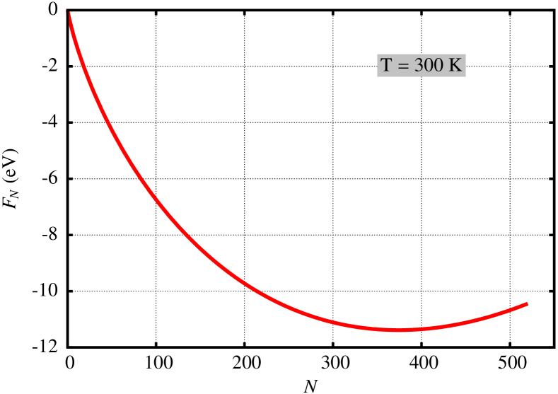
Figure 1: Helmholtz free energy for $L_{x}=L_{y}=100$ nm.

Extracted from the recurrence relation (23), the Helmholtz free energy is plotted in Fig. (1) versus the number of electrons $N$, up to $N=520$ beyond which sign changes (due to $\xi=-1$ for fermions) made the recurrence relation unstable. It turns out that, for fixed $L_{x}=L_{y}$, the free energy attains a minimum for a particular value of $N$ – in the present case around $N=374$ – which corresponds to $\muup_{N}=0$ or, equivalently, the absence of energy cost when a single particle is to be added or removed. On the other hand, a typical value of the areal electron concentration in a MOS capacitor operating at room temperature is $10^{12}$ cm^-2 which, for $L_{x}=L_{y}=100$ nm, corresponds to $N\approx 100$ and, hence, to a negative chemical potential.

Unlike $\muup_{N}$, the grand-canonical chemical potential $\muup_{\mathrm{GCE}}$ that corresponds to the thermodynamic limit $N\to\infty,L_{x},L_{y}\to\infty$, whilst $n_{\mathrm{S}}\equiv N/(L_{x}L_{y})$ remains finite, can be calculated analytically from

$$\muup_{\mathrm{GCE}}=\frac{1}{\beta}\ln\left(\exp\left(\frac{2\pi\beta\hbar^{2}n_{\mathrm{S}}}{m}\right)-1\right).$$ (38)

For the sake of comparison we have plotted both $\muup_{N}$ and $\muup_{\mathrm{GCE}}$ versus $N$ in Fig. 2 and in Fig. 3.

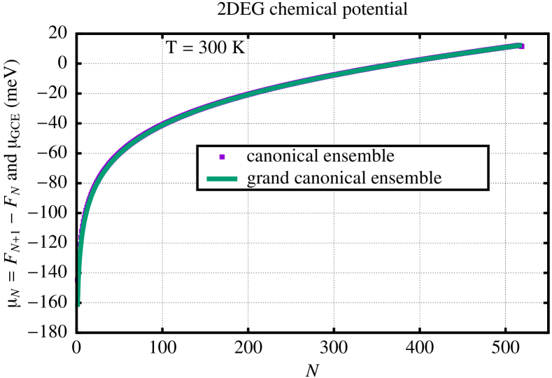
Figure 2: Canonical and grand-canonical chemical potentials for $L_{x}=L_{y}=100$ nm up to $N=520$.

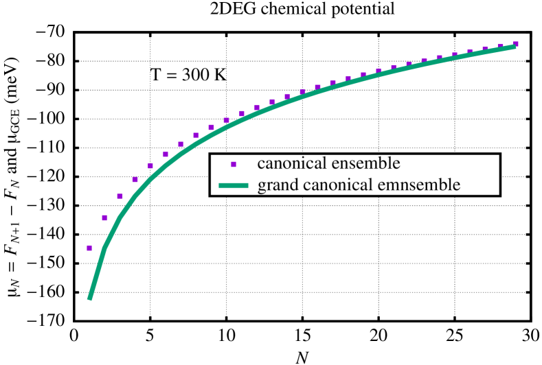
Figure 3: Canonical and grand-canonical chemical potentials for $L_{x}=L_{y}=100$ nm up to $N=30$.

For relatively large values of $N$, say $N>30$, $\muup_{N}$ and $\muup_{\mathrm{GCE}}$ are about equal. On the other hand, the expression (38) for $\muup_{\mathrm{GCE}}$ is only valid in the thermodynamic limit. It fails to characterize electron ensembles with $N\leqslant 30$ which can, however, be handled by the canonical formalism yielding $\muup_{N}$.

Moreover, in the case of more complicated fermionic systems, such as the 3DEG, the transcendental equation (26) expressing the (average) number of fermions in terms of $\muup_{\mathrm{GCE}}$ generally can no longer be inverted analytically, while the computational scheme that yields $\muup_{N}$ remains unaltered.

6 Correlation functions

So far we have concentrated on the projection operator approach for obtaining the partition function and derived quantities of indistinguishable particles, with particular attention to non-interacting particles. Two specific examples were worked out. But, as already mentioned in the Introduction, not just the partition function and its derived quantities but also single- and two-particle correlation functions of non-interacting particles are instrumental to perturbative and variational methods that are commonly entering approximative treatments of interacting particles. In the present section, it is shown that the projection operator is also well equipped to calculate these quantities.

Single- and two-particle correlation functions – also referred to as two-point and four-point functions – typically provide a signature of the correlation between particles that are spatially separated. For the sake of notational simplicity, positions in space are denoted by $x$ and $x^{\prime}$ which, however, should not at all be regarded as a limitation to strictly one-dimensional systems.
Considered quantum statistical averages, correlation functions are conveniently expressed in terms of field operators $\psi(x)$ satisfying typical (anti)commutation relations $\{\psi(x),\psi^{\dagger}(x^{\prime})\}=\delta(x-x^{\prime})$ etc.

6.1 Single-particle correlation functions

Adopting once again the canonical ensemble framework, we can reinvoke the above defined projection operator $\hat{\mathsf{P}}_{\!N}$ to calculate the single-particle correlation function (two-point function) for an ensemble of $N$ particles from

$$S_{\!2}(x,x^{\prime})=\mathinner{\langle{\psi^{\dagger}(x)\,\psi(x^{\prime})}\rangle}\equiv\frac{1}{Z_{N}}\mathsf{Tr}\left(\hat{\mathsf{P}}_{\!N}\exp(-\beta\,\hat{\mathsf{H}})\,\psi^{\dagger}(x)\,\psi(x^{\prime})\right).$$ (39)

In most cases of interest, both the single-particle energies $\epsilon^{\vphantom{\dagger}}_{k}$ and the corresponding single-particle wave functions $\phi_{k}(x)$ are supposed to be explicitly known, the latter constituting a complete, orthonormal basis. Hence, it proves convenient to expand the field operators as

$$\psi(x^{\prime})=\sum_{k^{\prime}}\phi_{k^{\prime}}(x^{\prime})\,c^{\vphantom{\dagger}}_{k^{\prime}},\quad\psi^{\dagger}(x)=\sum_{k}\phi^{*}_{k}(x)\,c^{\dagger}_{\!k},$$ (40)

the creation and destruction operators thereby appearing as expansion coefficients. Substitution into (39) yields

$$S_{\!2}(x,x^{\prime})=\sum_{kk^{\prime}}\phi^{*}_{k}(x)\,\phi_{k^{\prime}}(x^{\prime})\mathinner{\langle{c^{\dagger}_{\!k}c^{\vphantom{\dagger}}_{k^{\prime}}}\rangle}$$ (41)

with

$$\mathinner{\langle{c^{\dagger}_{\!k}c^{\vphantom{\dagger}}_{k^{\prime}}}\rangle} =\frac{1}{Z_{N}}\mathsf{Tr}\left(\hat{\mathsf{P}}_{\!N}\exp\left(-\beta\,\hat{\mathsf{H}}\right)c^{\dagger}_{\!k}c^{\vphantom{\dagger}}_{k^{\prime}}\right)$$

$$=\frac{1}{2\pi Z_{N}}\int_{-\pi}^{\pi}\!\!\mathrm{d}\theta\,\exp\left(-\mathrm{i}N\theta\right)\mathsf{Tr}\left(\exp\left(\mathrm{i}\theta\hat{\mathsf{N}}-\beta\,\hat{\mathsf{H}}\right)c^{\dagger}_{\!k}c^{\vphantom{\dagger}}_{k^{\prime}}\right)$$

$$=\frac{1}{2\pi Z_{N}}\int_{-\pi}^{\pi}\!\!\mathrm{d}\theta\,\exp\left(-\mathrm{i}N\theta\right)\Lambda_{kk^{\prime}}(\theta).$$ (42)

In order to evaluate the trace

$$\Lambda_{kk^{\prime}}(\theta)=\mathsf{Tr}\left(\exp\left(\mathrm{i}\theta\,\hat{\mathsf{N}}-\beta\,\hat{\mathsf{H}}\right)c^{\dagger}_{\!k}c^{\vphantom{\dagger}}_{k^{\prime}}\right),$$ (43)

we first exploit its invariance under cyclic permutations to get

$$\Lambda_{kk^{\prime}}(\theta)=\mathsf{Tr}\left(c^{\vphantom{\dagger}}_{k^{\prime}}\exp\left(\mathrm{i}\theta\,\hat{\mathsf{N}}-\beta\,\hat{\mathsf{H}}\right)c^{\dagger}_{\!k}\right).$$ (44)

At this point, we insert the identity operator $\exp(\mathrm{i}\theta\,\hat{\mathsf{N}}-\beta\,\hat{\mathsf{H}})\exp(-\mathrm{i}\theta\,\hat{\mathsf{N}}+\beta\,\hat{\mathsf{H}})$ under the trace, in front of $c^{\vphantom{\dagger}}_{k^{\prime}}$,

$$\Lambda_{kk^{\prime}}(\theta)=\mathsf{Tr}\left(\exp\left(\mathrm{i}\theta\,\hat{\mathsf{N}}-\beta\,\hat{\mathsf{H}}\right)\exp\left(-\mathrm{i}\theta\,\hat{\mathsf{N}}+\beta\,\hat{\mathsf{H}}\right)c^{\vphantom{\dagger}}_{k^{\prime}}\exp\left(\mathrm{i}\theta\,\hat{\mathsf{N}}-\beta\,\hat{\mathsf{H}}\right)c^{\dagger}_{\!k}\right),$$ (45)

and apply the operator identity

$$\exp\left(-\mathrm{i}\theta\,\hat{\mathsf{N}}+\beta\,\hat{\mathsf{H}}\right)c^{\vphantom{\dagger}}_{k^{\prime}}\exp\left(\mathrm{i}\theta\,\hat{\mathsf{N}}-\beta\,\hat{\mathsf{H}}\right)=\exp\left(\mathrm{i}\theta-\beta\epsilon^{\vphantom{\dagger}}_{k^{\prime}}\right)c^{\vphantom{\dagger}}_{k^{\prime}}$$ (46)

that proves valid for non-interacting particles. Indeed, given the Hamiltonian $\hat{\mathsf{H}}=\sum_{k}\epsilon^{\vphantom{\dagger}}_{k}c^{\dagger}_{\!k}c^{\vphantom{\dagger}}_{\!k}$ both exponents in $\exp\left(-\mathrm{i}\theta\,\hat{\mathsf{N}}+\beta\,\hat{\mathsf{H}}\right)c^{\vphantom{\dagger}}_{k^{\prime}}\exp\left(\mathrm{i}\theta\,\hat{\mathsf{N}}-\beta\,\hat{\mathsf{H}}\right)$ are found to factorize while $c^{\vphantom{\dagger}}_{k^{\prime}}$ commutes with each factor but the $k^{\prime}$-th one. Consequently, all factors appearing in the right exponent other than the $k^{\prime}$-th one can be shifted to the left so as to neutralize their inverse counterparts. Hence, we are left with

$$\exp\left(-\mathrm{i}\theta\,\hat{\mathsf{N}}+\beta\,\hat{\mathsf{H}}\right)c^{\vphantom{\dagger}}_{k^{\prime}}\exp\left(\mathrm{i}\theta\,\hat{\mathsf{N}}-\beta\,\hat{\mathsf{H}}\right)=\exp\left(zc^{\dagger}_{k^{\prime}}c^{\vphantom{\dagger}}_{k^{\prime}}\right)c^{\vphantom{\dagger}}_{k^{\prime}}\exp\left(-zc^{\dagger}_{k^{\prime}}c^{\vphantom{\dagger}}_{k^{\prime}}\right),$$ (47)

where $z=\beta\epsilon^{\vphantom{\dagger}}_{k^{\prime}}-\mathrm{i}\theta$. Differentiation of $u_{k^{\prime}}(z)\equiv\exp\left(zc^{\dagger}_{k^{\prime}}c^{\vphantom{\dagger}}_{k^{\prime}}\right)c^{\vphantom{\dagger}}_{k^{\prime}}\exp\left(-zc^{\dagger}_{k^{\prime}}c^{\vphantom{\dagger}}_{k^{\prime}}\right)$ with respect to $z$ yields a first-order linear differential equation

$$\frac{\partial u_{k^{\prime}}(z)}{\partial z} =\exp\left(zc^{\dagger}_{k^{\prime}}c^{\vphantom{\dagger}}_{k^{\prime}}\right)\left[c^{\dagger}_{k^{\prime}}c^{\vphantom{\dagger}}_{k^{\prime}},c^{\vphantom{\dagger}}_{k^{\prime}}\right]\exp\left(-zc^{\dagger}_{k^{\prime}}c^{\vphantom{\dagger}}_{k^{\prime}}\right)$$

$$=-\exp\left(zc^{\dagger}_{k^{\prime}}c^{\vphantom{\dagger}}_{k^{\prime}}\right)c^{\vphantom{\dagger}}_{k^{\prime}}\exp\left(-zc^{\dagger}_{k^{\prime}}c^{\vphantom{\dagger}}_{k^{\prime}}\right)=-u_{k^{\prime}}(z)$$ (48)

to be solved with the boundary condition $u_{k^{\prime}}(0)=c_{k^{\prime}}$. The trivial solution $u_{k^{\prime}}(z)=\exp\left(-z\right)c_{k^{\prime}}$ immediately leads to the operator identity quoted in Eq. (46).
As a result, we obtain

$$\Lambda_{kk^{\prime}}(\theta)=\exp\left(\mathrm{i}\theta-\beta\epsilon^{\vphantom{\dagger}}_{k^{\prime}}\right)\mathsf{Tr}\left(\exp\left(\mathrm{i}\theta\,\hat{\mathsf{N}}-\beta\,\hat{\mathsf{H}}\right)c^{\vphantom{\dagger}}_{k^{\prime}}c^{\dagger}_{\!k}.\right).$$ (49)

Exploiting $c^{\vphantom{\dagger}}_{k^{\prime}}c^{\dagger}_{\!k}=\delta^{\vphantom{\dagger}}_{k^{\prime}k}+\xi c^{\dagger}_{\!k}c^{\vphantom{\dagger}}_{k^{\prime}}$, we can rewrite the above results as

$$\Lambda_{kk^{\prime}}(\theta) =\exp\left(\mathrm{i}\theta-\beta\epsilon^{\vphantom{\dagger}}_{k^{\prime}}\right)\left[\delta_{kk^{\prime}}G(\beta,\theta)+\xi\mathsf{Tr}\left(\exp\left(\mathrm{i}\theta\hat{\mathsf{N}}-\beta\,\hat{\mathsf{H}}\right)c^{\dagger}_{\!k}c^{\vphantom{\dagger}}_{k^{\prime}}\right)\right]$$

$$=\exp\left(\mathrm{i}\theta-\beta\epsilon^{\vphantom{\dagger}}_{k^{\prime}}\right)\left[\delta_{kk^{\prime}}G(\beta,\theta)+\xi\Lambda_{kk^{\prime}}(\theta)\right].$$ (50)

Hence, the trivial solution reads

$$\Lambda_{kk^{\prime}}(\theta)=\delta_{k^{\prime}k}\frac{G(\beta,\theta)}{\exp\left(\beta\epsilon^{\vphantom{\dagger}}_{k}\!-\mathrm{i}\theta\right)-\xi}$$ (51)

In turn, the expression for the single-particle correlation function simplifies to

$$S_{\!2}(x,x^{\prime})=\frac{1}{2\pi Z_{N}}\sum_{k}\phi^{*}_{k}(x)\phi_{k}(x^{\prime})\int_{-\pi}^{\pi}\!\!\mathrm{d}\theta\,\exp\left(-\mathrm{i}N\theta\right)\frac{G(\beta,\theta)}{\exp\left(\beta\epsilon^{\vphantom{\dagger}}_{k}-\mathrm{i}\,\theta\right)-\xi}$$ (52)

with the particle density $n(x)=S_{\!2}(x,x)$ emerging as a particular case.

6.2 Pair correlation functions

Introducing the pair correlation function (four point function) as

$$S_{\!4}(x,x^{\prime})=\mathinner{\langle{\psi^{\dagger}(x)\,\psi(x)\,\psi^{\dagger}(x^{\prime})\,\psi(x^{\prime})}\rangle},$$ (53)

we first write $S_{\!4}(x,x^{\prime})$ as

$$S_{\!4}(x,x^{\prime}) =\mathinner{\langle{\psi^{\dagger}(x)\,\psi(x^{\prime})}\rangle}\delta(x-x^{\prime})+\mathinner{\langle{\psi^{\dagger}(x)\,\psi^{\dagger}(x^{\prime})\,\psi(x^{\prime})\,\psi(x)}\rangle}$$

$$=n(x)\,\delta(x-x^{\prime})+\mathinner{\langle{\psi^{\dagger}(x)\,\psi^{\dagger}(x^{\prime})\,\psi(x^{\prime})\,\psi(x)}\rangle}.$$ (54)

Expanding again all field operators in the complete set $\{\phi_{k}(x)\}$, we obtain

$$\mathinner{\langle{\psi^{\dagger}(x)\,\psi^{\dagger}(x^{\prime})\,\psi(x^{\prime})\,\psi(x)}\rangle}=\sum_{kk^{\prime}}\sum_{qq^{\prime}}\phi^{*}_{q}(x)\,\phi^{*}_{q^{\prime}}(x^{\prime})\phi_{k^{\prime}}(x^{\prime})\,\phi_{k}(x)\mathinner{\langle{c^{\dagger}_{q}\,c^{\dagger}_{q^{\prime}}\,c^{\vphantom{\dagger}}_{k^{\prime}}\,c^{\vphantom{\dagger}}_{\!k}}\rangle}.$$ (55)

A lengthy but straightforward calculation involving another application of the operator identity (46) and the commutation relation $[c^{\vphantom{\dagger}}_{\!k},c^{\dagger}_{q}\,c^{\dagger}_{q^{\prime}}]=\delta_{kq}c^{\dagger}_{q^{\prime}}+\xi\delta_{kq^{\prime}}c^{\dagger}_{q}$ leads to

$$\mathinner{\langle{c^{\dagger}_{q}\,c^{\dagger}_{q^{\prime}}\,c^{\vphantom{\dagger}}_{k^{\prime}}\,c^{\vphantom{\dagger}}_{\!k}}\rangle}=\frac{1}{2\pi Z_{N}}\left(\xi\delta_{kq}\delta_{k^{\prime}q^{\prime}}+\delta_{kq^{\prime}}\delta_{k^{\prime}q}\right)\int_{-\pi}^{\pi}\!\!\mathrm{d}\theta\,\exp\left(-\mathrm{i}N\theta\right)\\ \times\frac{G(\beta,\theta)}{\left(\exp\left(\beta\epsilon^{\vphantom{\dagger}}_{k}-\mathrm{i}\theta\right)-\xi\right)\left(\exp\left(\beta\epsilon^{\vphantom{\dagger}}_{k^{\prime}}-\mathrm{i}\theta\right)-\xi\right)}.$$ (56)

Correspondingly, the pair correlation function is given by

$$\mathinner{\langle{\psi^{\dagger}(x)\,\psi^{\dagger}(x^{\prime})\,\psi(x^{\prime})\,\psi(x)}\rangle}=\frac{\xi^{N}}{2\pi Z_{N}}\sum_{kk^{\prime}}\left(\xi|\phi_{k}(x)|^{2}|\phi_{k^{\prime}}(x^{\prime})|^{2}+\phi^{*}_{k^{\prime}}(x)\,\phi^{*}_{k}(x^{\prime})\phi_{k^{\prime}}(x^{\prime})\,\phi_{k}(x)\right)\\ \times\int_{-\pi}^{\pi}\!\!\mathrm{d}\theta\,\exp\left(-\mathrm{i}N\theta\right)\frac{G(\beta,\theta)}{\left(\exp\left(\beta\epsilon^{\vphantom{\dagger}}_{k}-\mathrm{i}\theta\right)-\xi\right)\left(\exp\left(\beta\epsilon^{\vphantom{\dagger}}_{k^{\prime}}-\mathrm{i}\theta\right)-\xi\right)}$$ (57)

Appendix A Principle of maximum entropy

Consider the density operator

$$\hat{\rho}_{N}=\sum_{j}p_{j,N}\mathinner{|\psi_{j,N}\rangle\langle\psi_{j,N}|}\quad\text{with}\quad\sum_{j}p_{j,N}=1,$$ (58)

where $p_{j,N}$ is the probability that state $|\psi_{j,N}\rangle$ of the $N-$particle subspace is occupied in thermal equilibrium, i.e. with a fixed ensemble average $U_{\!N}$ for the energy [6, 7, 8]:

$$U_{\!N}=\mathsf{Tr}\left(\hat{\mathsf{H}}_{N}\hat{\rho}_{N}\right)=\sum_{j}p_{j,N}E_{\!j,N}.$$ (59)

Maximizing the entropy

$$S_{\!N}=-k_{\mathrm{B}}\mathsf{Tr}\left(\hat{\rho}_{N}\ln\hat{\rho}_{N}\right)=-k_{\mathrm{B}}\sum_{j}p_{j,N}\ln p_{j,N}$$ (60)

imposes

$$-k_{\mathrm{B}}\frac{\partial}{\partial p_{j,N}}\sum_{j^{\prime}}p_{j^{\prime},N}\left(\ln p_{j^{\prime},N}+\alpha+\beta E_{\!j^{\prime},N}\right)=0,$$ (61)

where $\alpha$ and $\beta$ are Lagrange multipliers for the normalization and the energy condition, respectively. Hence $p_{j,N}=\frac{1}{Z_{N}}\mathrm{e}^{-\beta E_{\!j,N}}$ with $Z_{N}=\sum_{j}\mathrm{e}^{-\beta E_{\!j,N}}$. But, keeping in mind that $Z_{N}$ and $\beta$ are in fact functions of the fixed value $U_{\!N}$, a more careful notation is introduced:

$$p_{j,N}(U_{\!N})=\frac{1}{Z_{N}(U_{\!N})}\mathrm{e}^{-\beta(U_{\!N})E_{\!j,N}},\qquad Z_{N}(U_{\!N})=\sum_{j}\mathrm{e}^{-\beta(U_{\!N})E_{\!j,N}},$$ (62)

and therefore

$$U_{\!N} =\frac{1}{Z_{N}(U_{\!N})}\sum_{j}E_{\!j,N}\mathrm{e}^{-\beta(U_{\!N})E_{\!j,N}},$$ (63)

$$S_{\!N}(U_{\!N} =k_{\mathrm{B}}\ln Z_{N}(U_{\!N})+k_{\mathrm{B}}\beta(U_{\!N})U_{\!N}.$$ (64)

where the equation for $U_{\!N}$ is a transcendental equation which determines the Lagrange multiplier $\beta$, and hence the temperature $T$ if defined as $\beta=1/(k_{\mathrm{B}}T)$. The Helmholtz free energy

$$F_{\!N}(U_{\!N})\equiv U_{\!N}-\frac{1}{k_{\mathrm{B}}\beta(U_{\!N})}S_{\!N}(U_{\!N})$$ (65)

then becomes, as expected:

$$F_{\!N}(U_{\!N})\equiv-\frac{1}{\beta(U_{\!N})}\ln Z_{N}(U_{\!N}).$$ (66)

At first glance all these result are familiar. Less familiar is a relationship between the entropy and the energy dependence of $\beta$. Differentiating $Z_{N}$ with respect to $U_{\!N}$, one obtains $\mathrm{d}\ln Z_{N}/\mathrm{d}U_{\!N}=-U_{\!N}\mathrm{d}\beta/\mathrm{d}U$, and hence

$$\ln Z_{N}(U_{\!N})-\ln Z_{N}(U_{0})=-U_{\!N}\beta(U_{\!N})+U_{0}\beta(U_{0})+\int_{U_{0}}^{U_{\!N}}\!\!\mathrm{d}U\,\beta(U).$$ (67)

Using (63–65), this expression simplifies into

$$S_{\!N}(U_{\!N})-S_{\!N}(U_{0})=k_{\mathrm{B}}\int_{U_{0}}^{U_{\!N}}\!\!\mathrm{d}U\,\beta(U),$$ (68)

showing how the entropy increases with increasing internal energy. In the classical limit, with $\beta(U)=C/(k_{\mathrm{B}}U)$ where $C$ is the specific heat, the right hand side becomes $C\ln(U_{\!N}/U_{0})=C\ln(T_{N}/T_{0})$, consistent with the equipartition theorem.

So far, it was shown that the projection operator approach is consistent with the standard interrelations between the thermodynamic quantities, all derivable from the partition function $Z_{N}$ and the (given) internal energy $U_{\!N}$. No attention was paid to the relevance of the projection operator for the actual calculation of $Z_{N}$, which becomes now the main topic of interest. Since $\mathsf{\hat{P}}_{N}^{2}=\hat{\mathsf{P}}_{\!N}$, and $Z_{N}$ can be rewritten as $Z_{N}=\mathsf{Tr}(\mathrm{e}^{-\beta\hat{\mathsf{H}}_{N}})$, one obtains with little effort from (62)

$$Z_{N}(U_{\!N})=\mathsf{Tr}\left(\mathrm{e}^{-\beta(U_{\!N})\hat{\mathsf{H}}}\hat{\mathsf{P}}_{\!N}\right),$$ (69)

regardless whether the particles are interacting or not. Without the projection operator, this would be the grand canonical partition function, for which the chemical potential is required as a Lagrange multiplier to impose the average number of particles. The present approach is bound to work in the canonical ensemble with exactly $N$ particles.

Until this point, a purist notation was followed, emphasizing that thermal equilibrium means that the internal energy $U_{\!N}$ is fixed, and that a Lagrange multiplier $\beta(U_{\!N})$ is introduced in (63) to fulfill this requirement [6, 7, 8]. For practical purposes, this formal treatment is less appropriate. It is much easier to consider $\beta$ as a function argument

$$Z_{N}(\beta)=\mathsf{Tr}\left(\mathrm{e}^{-\beta\hat{\mathsf{H}}}\hat{\mathsf{P}}_{\!N}\right),$$ (70)

which at the end of the calculations is connected to the internal energy via

$$U_{\!N}(\beta)=\frac{1}{Z_{N}(\beta)}\mathsf{Tr}\left(\hat{\mathsf{H}}\mathrm{e}^{-\beta\hat{\mathsf{H}}}\hat{\mathsf{P}}_{\!N}\right)=-\frac{\mathrm{d}}{\mathrm{d}\beta}\ln\left(Z_{N}(\beta)\right).$$ (71)

Appendix B Two Euler identities

Given two complex numbers $z$ and $q$, with $|q|<1$, Leonhard Euler in the 18th century derived (amongst a variety of other mathematical insights) the following two identities:

$$\prod_{n=0}^{\infty}\frac{1}{1-zq^{n}} =1+\sum_{n=1}^{\infty}z^{n}\prod_{k=1}^{n}\frac{1}{1-q^{k}}$$ (72)

$$\prod_{n=0}^{\infty}\left(1-zq^{n}\right) =1+\sum_{n=1}^{\infty}z^{n}(-1)^{n}q^{n(n-1)/2}\prod_{k=1}^{n}\frac{1}{1-q^{k}},$$ (73)

In contemporary literature [13, 14, 15, 16], they are usually obtained as a by-product of more general theorems on $q$-products and $q$-series, which hinders a transparent derivation. Therefore we propose an easily accessible proof, inspired by a strategy of Berndt [16]. Given a set of complex numbers $a,b,q,z$ with $|z|<1,|az|<1,|bz|<1,|q|<1$, define a function

$$f(z)=\prod_{n=0}^{\infty}\frac{1-azq^{n}}{1-bzq^{n}}$$ (74)

and calculate $f(qz)$,

$$f(qz)=\prod_{n=0}^{\infty}\frac{1-azq^{n+1}}{1-bzq^{n+1}}=\prod_{n=1}^{\infty}\frac{1-azq^{n}}{1-bzq^{n}}=\frac{1-bz}{1-az}\prod_{n=0}^{\infty}\frac{1-azq^{n}}{1-bzq^{n}}=\frac{1-bz}{1-az}f(z).$$ (75)

The latter can conveniently be rewritten as

$$f(z)-f(qz)=bzf(z)-azf(qz).$$ (76)

Since $f(z)$ is analytic wherever $|z|<1$, we may assign a power series to it:

$$f(z)=\sum_{n=0}^{\infty}C_{n}z^{n},$$ (77)

where $C_{0}=f(0)=1$ holds by construction of $f(z)$.
Substituting (77) into (76), we obtain

$$\sum_{n=0}^{\infty}C_{n}\left(1-q^{n}\right)z^{n}=\sum_{n=0}^{\infty}C_{n}\left(b-aq^{n}\right)z^{n+1}.$$ (78)

Clearly, the $n=0$ term in the left-hand side of Eq. (78) vanishes, while its right-hand side may be rephrased by shifting the summation index $n+1\to n$, yielding

$$\sum_{n=1}^{\infty}C_{n}\left(1-q^{n}\right)z^{n}=\sum_{n=1}^{\infty}C_{n-1}\left(b-aq^{n-1}\right)z^{n}.$$ (79)

Identification of the coefficients of $z^{n}$ then leads to the recurrence relation

$$C_{n}=\frac{b-aq^{n-1}}{1-q^{n}}\,C_{n-1},\qquad n\geqslant 1,$$ (80)

which can be solved with the help of $C_{0}=1$ to get

$$C_{n}=\prod_{k=1}^{n}\frac{b-aq^{k-1}}{1-q^{k}},$$ (81)

Filling $C_{n}$ out in (77) gives a generalization of the well-known $q$-binomial theorem

$$\prod_{n=0}^{\infty}\frac{1-azq^{n}}{1-bzq^{n}}=1+\sum_{n=1}^{\infty}z^{n}\prod_{k=1}^{n}\frac{b-aq^{k-1}}{1-q^{k}}$$ (82)

The Euler identities (72) and (73) emerge as special cases of (82), corresponding respectively to the cases $a=0,b=1$ and $a=1,b=0$.

References

References

- [1] B. Robertson, Introduction to field operators in quantum mechanics, American Journal of Physics 41 (1973) 678 – 690.
- [2] H.-T. Elze, W. Greiner, Quantum statistics with internal symmetry, Physical Review A 33 (1986) 1879 – 1891.
- [3] H.-T. Elze, W. Greiner, Finite size effects for quark-gluon plasma droplets, Physics Letters B 179 (1986) 385.
- [4] H.-T. Elze, D. Miller, K. Redlich, Gauge theories at finite temperature and chemical potential, Physics Review D 35 (1987) 748.
- [5] M. Bender, P. H. Heenen, P. G. Reinhard, Self-consistent mean-field models for nuclear structure, Review of Modern Physics 75 (2003) 121 – 180.
- [6] E. T. Jaynes, Information theory and statistical mechanics, Physical Review 106 (1957) 620 – 630.
- [7] E. T. Jaynes, Information theory and statistical mechanics, ii, Physical Review 108 (1957) 171 – 190.
- [8] W. T. Grandy, Entropy and the Time Evolution of Macroscopic Systems, Oxford University Press, 2008.
- [9] R. P. Feynman, Statistical Mechanics, W. A. Benjamin, Inc., 1972.
- [10] H. Kleinert, Path integrals in Quantum Mechanics, Statistics, Polymer Physics, and Financial Markets, 3rd Edition, World Scientific, New Jersey, 2004.
- [11] P. T. Landsberg, Thermodynamics, Interscience, New York, 1961.
- [12] P. Borrmann, G. Franke, Recursion formulas for quantum statistical partition functions, Journal of Chemical Physics 98 (1993) 2484 – 2485.
- [13] G. E. Andrews, A simple proof of Jacobi’s triple product identity, Proceedings of the American Mathematical Society 16 (1965) 333 – 334.
- [14] R. Bellman, A brief introduction to theta functions, Holt, Rinehart and Winston, New York, 1961.
- [15] G. Gasper, M. Rahman, Basic Hypergeometric Series, Encyclopedia of Mathematics and Its Applications 96, Second Edition, Cambridge University Press, Cambridge, 2004.
- [16] B. C. Berndt, Number theory in the spirit of Ramanujan, Student Mathematical Library, Vol. 34, American Mathematical Society, Providence, 2006.