Numerical computation of the conformal map onto lemniscatic domains

Abstract

We present a numerical method for the computation of the conformal map from unbounded multiply-connected domains onto lemniscatic domains. For $\ell$-times connected domains the method requires solving $\ell$ boundary integral equations with the Neumann kernel. This can be done in $O(\ell^{2}n\log n)$ operations, where $n$ is the number of nodes in the discretization of each boundary component of the multiply connected domain. As demonstrated by numerical examples, the method works for domains with close-to-touching boundaries, non-convex boundaries, piecewise smooth boundaries, and for domains of high connectivity.

Keywords numerical conformal mapping; multiply connected domains; lemniscatic domains; boundary integral equations; Neumann kernel.

Mathematics Subject Classification (2010) 30C30; 45B05; 65E05

1 Introduction

In the theory of conformal mapping for multiply connected domains (open and connected sets) in the extended complex plane $\widehat{\mathbb{C}}=\mathbb{C}\cup\{\infty\}$, there are several canonical domains onto which a given domain may be mapped. The most commonly considered canonical domains are slit domains (see, e.g., Chapter VIII in the book of Nehari [39]), circular domains, and domains with polygonal boundary. Conformal maps onto these domains have been intensively studied, and several numerical methods for the computation of these maps have been proposed. Slit domains are considered, e.g., in [1, 6, 9, 30, 31, 32, 33], circular domains in [7, 28, 34], and Schwarz–Christoffel maps for polygonal domains in [4, 5, 7, 8, 10, 11, 12] .

In this article we consider the numerical computation of the conformal map onto lemniscatic domains, which are another type of canonical domain. A lemniscatic domain is a domain of the form

$$\mathcal{L}\mathrel{\mathop{:}}=\Big{\{}w\in\widehat{\mathbb{C}}:\prod_{j=1}^{\ell}|w-a_{j}|^{m_{j}}>\tau\Big{\}},$$ (1)

where $a_{1},\ldots,a_{\ell}\in\mathbb{C}$ are pairwise distinct, $m_{1},\ldots,m_{\ell},\tau>0$ are real numbers, and the exponents satisfy

$$\sum_{j=1}^{\ell}m_{j}=1.$$ (2)

Lemniscatic domains where introduced by Walsh [44], who proved that if $\mathcal{K}$ is an $\ell$-times connected domain with $\infty\in\mathcal{K}$, there exists a lemniscatic domain $\mathcal{L}$ as in (1) and a conformal map $\Phi:\mathcal{K}\to\mathcal{L}$ normalized by $\Phi(\infty)=\infty$ and $\Phi^{\prime}(\infty)=1$; see Theorem 2.1 below for the precise statement. The conformal map onto a lemniscatic domain is a direct generalization of the Riemann map for simply connected domains, for if $\ell=1$ in (1), then $\mathcal{L}$ is is the exterior of a disk.

In addition to Walsh [44], the existence of the conformal map onto a lemniscatic domain was shown by Grunsky [16, 17], Jenkins [20] and Landau [26]. The last paper also contains an iteration method for computing $\Phi$, which, however, requires knowledge of the harmonic measure of parts of the boundary of the original domain $\mathcal{K}$. Recently, two of the present authors have investigated properties of this map and constructed some explicit examples in [42].

A remarkable feature of Walsh’s conformal map is that it allows a direct generalization of the classical Faber polynomials, which are defined for simply connected compact sets, to compact sets with several components. The resulting Faber–Walsh polynomials, introduced by Walsh in [45], are likely to prove useful, given the vast number of both theoretical and practical applications of the classical Faber polynomials. For further details on Faber–Walsh polynomials we refer to the recent paper [43].

Since the construction of conformal maps onto lemniscatic domains is in general nontrivial and only a few explicit examples are known, it is desirable to have a method for numerically computing such maps. In this paper we derive such a method and study it numerically. More precisely, given an $\ell$-times connected domain $\mathcal{K}$ with a sufficiently smooth boundary our method computes the parameters defining the corresponding lemniscatic domain $\mathcal{L}$ as well as the boundary values of the conformal map $\Phi:\mathcal{K}\to\mathcal{L}$. The method can be considered an extension of the approach described in [30, 31, 32, 33] for the computation, in a unified way, of conformal maps onto all $39$ slit domains identified by Koebe in [23]. The method described in [30, 31, 32, 33] requires solving a boundary integral equation with the generalized Neumann kernel. Using the Fast Multipole Method (FMM), the integral equation for multiply connected domains of connectivity $\ell$ can be solved numerically in $O(\ell n\log n)$ operations where $n$ is the number of nodes in the discretization of each boundary component [35, 36]. The method presented in this article requires solving $\ell$ boundary integral equations followed by solving a system of $\ell n+\ell$ non-linear equations. The values of the conformal map $\Phi$ for interior points can then be calculated using Cauchy’s integral formula.

In recent years, several numerical methods have been proposed for computing the conformal map of multiply connected domains onto different types of canonical domains; see [1, 4, 5, 6, 7, 8, 9, 10, 11, 12, 28, 30, 31, 32, 33, 34, 36, 47, 49] and the references cited therein. However, most of these numerical methods are limited to certain types of canonical domains or original domains. In comparison, the approach using the boundary integral equation with the generalized Neumann kernel can be used for a wide range of canonical domains. Moreover, it has been successfully applied to domains of very high connectivity, with piecewise smooth boundaries, with close-to-touching boundaries, and with complex geometry; see [36, 34, 35, 38].

This paper is organized as follows. In Section 2 we state Walsh’s existence theorem for the conformal map onto lemniscatic domains. We then give the definition of the Neumann kernel in Section 3. In Section 4 we derive equations for the boundary values of the conformal map $\Phi$ and for the parameters of the lemniscatic domain $\mathcal{L}$. In Section 5 we use these equations for the derivation of a numerical method for computing $\Phi$ and $\mathcal{L}$. Numerical examples with five different domains are presented in Section 6. Concluding remarks are given in Section 7.

2 The conformal map onto lemniscatic domains

The following result is Walsh’s existence theorem from [44] (see also [26, Theorem 4]), which shows that lemniscatic domains are canonical domains for certain $\ell$-times connected domains.

Theorem 2.1.

Let $\mathcal{K}$ be an unbounded domain in $\widehat{\mathbb{C}}$ with $\infty\in\mathcal{K}$, and let $\Gamma=\partial\mathcal{K}$ consist of $\ell$ closed Jordan curves $\Gamma_{1},\ldots,\Gamma_{\ell}$. Then there exist a uniquely determined lemniscatic domain $\mathcal{L}$ of the form (1) and a uniquely determined bijective and conformal map

$$\Phi:\mathcal{K}\to\mathcal{L}\quad\text{ with }\quad\Phi(z)=z+O\left(\frac{1}{z}\right)\;\text{ near infinity.}$$ (3)

Further $\Phi$ extends to a continuous bijective map from $\overline{\mathcal{K}}=\mathcal{K}\cup\Gamma$ to $\overline{\mathcal{L}}$, and for each $j=1,\ldots,\ell$, the image of $\Gamma_{j}$ under $\Phi$ contains the point $a_{j}$ in its interior.

The number $\tau>0$ is the transfinite diameter (i.e., the logarithmic capacity) of the compact set $\widehat{\mathbb{C}}\backslash\mathcal{K}$.

The uniqueness of the lemniscatic domain and the conformal map in Theorem 2.1 is forced by the normalization condition of $\Phi$ near infinity expressed in (3). Note that if $c\in\mathbb{C}$ is any constant, then $\Phi_{c}=\Phi+c$ maps $\mathcal{K}$ bijectively and conformally onto the translated lemniscatic domain $\mathcal{L}+c$, and $\Phi_{c}$ satisfies the normalization conditions $\Phi_{c}(\infty)=\infty$ and $\Phi_{c}^{\prime}(\infty)=1$.

Theorem 2.1 is illustrated in Figure 1 for a domain $\mathcal{K}$ bounded by three Jordan curves; see Example 6.5 in Section 6 for details.

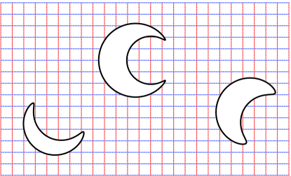
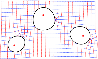
Figure 1: Illustration of Theorem 2.1. Original domain (left) and corresponding lemniscatic domain (right). The red dots are the centers $a_{1},a_{2},a_{3}$.

We will need the following lemma.

Lemma 2.2.

In the notation of Theorem 2.1, let

$$U(w)=\prod_{j=1}^{\ell}(w-a_{j})^{m_{j}},$$

so that $\mathcal{L}=\{w\in\widehat{\mathbb{C}}:|U(w)|>\tau\}$. Then $U^{\prime}(w)\neq 0$ for $w\in\partial\mathcal{L}=\{w\in\widehat{\mathbb{C}}:|U(w)|=\tau\}$.

Proof.

We show that the zeros of $U^{\prime}$ are the critical points of a Green’s function with pole at infinity, and that these are not located on $\partial\mathcal{L}$.

The function $U$ is analytic but multi-valued in $\mathbb{C}\backslash\{a_{1},\ldots,a_{\ell}\}$. Let $0<\rho<\tau$ and consider the auxiliary function

$$F(w)=\log U(w)-\log(\rho),$$

which is analytic but not single-valued in $\mathbb{C}\backslash\{a_{1},\ldots,a_{\ell}\}$. Then the harmonic functions

$$G(w)=\operatorname{Re}(F(w))=\log|U(w)|-\log(\rho)\quad\text{ and }\quad H(w)=\operatorname{Im}(F(w))$$

are conjugates, i.e., $G_{x}=H_{y}$ and $G_{y}=-H_{x}$. The derivative of $F$ is given by

$$\frac{U^{\prime}}{U}=F^{\prime}=\frac{1}{2}(F_{x}-iF_{y})=\frac{1}{2}(G_{x}+iH_{x}-i(G_{y}+iH_{y}))=G_{x}-iG_{y}.$$

Since $G$ is real-valued, $U^{\prime}(w_{0})=0$ if and only if $G_{x}(w_{0})=0=G_{y}(w_{0})$, i.e., the zeros of $U^{\prime}$ are the critical points of $G$.

The function $G$ is Green’s function with pole at infinity for the $\ell$-times connected domain $\{w\in\widehat{\mathbb{C}}:|U(w)|>\rho\}$, see [45, p. 28]. Its contour lines (level curves)

$$\Lambda_{\sigma}=\{w\in\mathbb{C}:G(w)=\log(\sigma)\}=\{w\in\mathbb{C}:|U(w)|=\sigma\rho\},\quad\sigma\geq 1,$$

have the following properties [46, p. 67]:

1. For sufficiently small $\sigma>1$, $\Lambda_{\sigma}$ consists of $\ell$ contours, each surrounding exactly one of the boundary contours (of $\{w\in\widehat{\mathbb{C}}:|U(w)|>\rho\}$).

2. $\Lambda_{\sigma}$ grows with $\sigma$, in the sense that if $\sigma<\sigma^{\prime}$, then $\Lambda_{\sigma}$ is contained in the interior of $\Lambda_{\sigma^{\prime}}$.

3. If $\sigma$ increases and $\Lambda_{\sigma}$ crosses through an $m$-fold critical point of $G$, the number of components of $\Lambda_{\sigma}$ decreases by exactly $m$.

Now, since $\mathcal{L}$ is $\ell$-times connected, $\partial\mathcal{L}=\Lambda_{\tau/\rho}$ has $\ell$ components. Therefore, no critical points of $G$ can lie on $\partial\mathcal{L}$ (or interior to $\partial\mathcal{L}$), which finishes the proof. ∎

3 The Neumann kernel

From now on we assume that $\mathcal{K}$ is a given domain as in Theorem 2.1 which additionally has a sufficiently smooth boundary $\Gamma$, oriented such that $\mathcal{K}$ is on the left of $\Gamma$. More precisely, we assume that each boundary curve $\Gamma_{j}$ is parameterized by a $2\pi$-periodic twice continuously differentiable complex function $\eta_{j}(t)$ with non-vanishing first derivative $\dot{\eta}_{j}(t)=d\eta_{j}(t)/dt\neq 0$ for $t\in J_{j}=[0,2\pi]$, $j=1,2,\ldots,\ell$. (A dot always denotes the derivative with respect to the parameter $t$.) The total parameter domain $J$ is the disjoint union of the $\ell$ intervals $J_{1},\ldots,J_{\ell}$,

$$J\mathrel{\mathop{:}}=\bigsqcup_{j=1}^{\ell}J_{j}=\bigcup_{j=1}^{\ell}\{(t,j)\;:\;t\in J_{j}\},$$

i.e., the elements of $J$ are ordered pairs $(t,j)$ where $j$ is an auxiliary index indicating which of the intervals contains the point $t$. We define a parametrization of the whole boundary $\Gamma$ as the complex function $\eta$ defined on $J$ by

$$\eta(t,j)\mathrel{\mathop{:}}=\eta_{j}(t),\quad t\in J_{j},\quad j=1,\ldots,\ell.$$ (4)

We shall assume for a given $t$ that the auxiliary index $j$ is known, so we replace the pair $(t,j)$ in the left-hand side of (4) by $t$. Thus, the function $\eta$ in (4) is written as

$$\eta(t)=\left\{\begin{array}[]{l@{\hspace{0.5cm}}l}\eta_{1}(t),\hfil\hskip 14.22636pt&t\in J_{1},\\ \hskip 8.5359pt\vdots\hfil\hskip 14.22636pt\\ \eta_{\ell}(t),\hfil\hskip 14.22636pt&t\in J_{\ell}.\\ \end{array}\right.$$

Let $H$ be the space of all real-valued Hölder continuous functions on the boundary $\Gamma$. In view of the smoothness of the parametrization $\eta(t)$ of the boundary $\Gamma$, any function $\phi\in H$ can be interpreted via $\hat{\phi}(t)\mathrel{\mathop{:}}=\phi(\eta(t))$ as a $2\pi$-periodic Hölder continuous function of the parameter $t$ on $J$, and vice versa. Henceforth, in this paper, we shall not distinguish between $\phi(t)$ and $\phi(\eta(t))$.

We define the Neumann kernel $N(s,t)$ for $(s,t)\in J\times J$ by

$$N(s,t)\mathrel{\mathop{:}}=\frac{1}{\pi}\mathop{\mathrm{Im}}\left(\frac{\dot{\eta}(t)}{\eta(t)-\eta(s)}\right).$$

It is a particular case of the generalized Neumann kernel considered in [48]. Similarly, the kernel $M(s,t)$ defined for $(s,t)\in J\times J$ by

$$M(s,t)\mathrel{\mathop{:}}=\frac{1}{\pi}\mathop{\mathrm{Re}}\left(\frac{\dot{\eta}(t)}{\eta(t)-\eta(s)}\right),$$

is a particular case of the kernel $M$ considered in [48]. The above kernels have been used in [31, 32] for computing the conformal map from unbounded multiply domains onto the canonical slit domains; see also [36, 35, 37]. The Neumann kernel also appears frequently in the integral equations for potential theory; see, e.g., [2, 13, 19, 25, 47].

Lemma 3.1 (see [48]).

(a) The kernel $N$ is continuous with

$$N(t,t)=\frac{1}{2\pi}\mathop{\mathrm{Im}}\frac{\ddot{\eta}(t)}{\dot{\eta}(t)}.$$

(b) When $s,t\in J_{j}$ are in the same parameter interval $J_{j}$, then

$$M(s,t)=-\frac{1}{2\pi}\cot\frac{s-t}{2}+M_{1}(s,t)$$

with a continuous kernel $M_{1}$ which takes on the diagonal the values

$$M_{1}(t,t)=\frac{1}{2\pi}\mathop{\mathrm{Re}}\frac{\ddot{\eta}(t)}{\dot{\eta}(t)}.$$

We define integral operators ${\bf N}$ and ${\bf M}$ on the space $H$ by

$${\bf N}\mu(s) \mathrel{\mathop{:}}=\int_{J}N(s,t)\mu(t)dt,\quad s\in J,$$

$${\bf M}\mu(s) \mathrel{\mathop{:}}=\int_{J}M(s,t)\mu(t)dt,\quad s\in J.$$

The integral operator ${\bf N}$ is a compact operator and the operator ${\bf M}$ is a singular operator. Both operators ${\bf N}$ and ${\bf M}$ are bounded on the space $H$ and map $H$ into itself [48]. Finally, any piecewise constant function $\nu\in H$ defined by

$$\nu(t)=\nu_{j}\quad{\rm for}\quad t\in J_{j},$$

with real constants $\nu_{j}$ for $j=1,\ldots,\ell$, will be denoted by

$$\nu(t)=(\nu_{1},\ldots,\nu_{\ell}),\quad t\in J.$$

4 The boundary values of $\Phi$ and the parameters of $\mathcal{L}$

In this section we derive equations for the boundary values of the conformal map $\Phi$ and for the parameters of the lemniscatic domain $\mathcal{L}$. These equations will be used for the numerical computation of $\Phi$ and $\mathcal{L}$ in Section 5 below.

In the notation of Theorem 2.1, the function $\Phi$ maps the boundary $\Gamma$ of ${\mathcal{K}}$ onto the boundary of the lemniscatic domain ${\mathcal{L}}$, i.e., for $t\in J$,

$$\prod_{j=1}^{\ell}|\Phi(\eta(t))-a_{j}|^{m_{j}}=\tau,$$

or, equivalently,

$$\sum_{j=1}^{\ell}m_{j}\log|\Phi(\eta(t))-a_{j}|=\log\tau.$$ (5)

To determine the parameters of the lemniscatic domain and the boundary values of $\Phi$, we fix for each $j=1,\ldots,\ell$ an auxiliary point $\alpha_{j}$ in the interior of the curve $\Gamma_{j}$, and define the functions

$$\gamma_{j}(t)\mathrel{\mathop{:}}=-\log|\eta(t)-\alpha_{j}|,\quad t\in J,\quad j=1,\ldots,\ell.$$ (6)

The first equation for the boundary values of $\Phi$ will be obtained from the boundary values of the function

$$f(z)=\sum_{j=1}^{\ell}m_{j}\log\left(\frac{\Phi(z)-a_{j}}{z-\alpha_{j}}\right),$$ (7)

where the branch of the logarithm with $\log(1)=0$ is chosen. The function $f$ is analytic in the domain ${\mathcal{K}}$ with $f(\infty)=0$. By (5), its boundary values are given by

$$f(\eta(t))=\log\tau+\gamma(t)+\mathrm{i}\mu(t),\quad t\in J,$$ (8)

where

$$\gamma(t) \mathrel{\mathop{:}}=\sum_{j=1}^{\ell}m_{j}\gamma_{j}(t)=-\sum_{j=1}^{\ell}m_{j}\log|\eta(t)-\alpha_{j}|,$$ (9)

$$\mu(t) \mathrel{\mathop{:}}=\mathop{\mathrm{Im}}f(\eta(t)).$$

Although the functions $\gamma_{j}$ are known from (6), the constant $\log\tau$ and the functions $\gamma$ and $\mu$ are not known a priori. We now show how the boundary values (8) of $f$ can be computed from the functions $\gamma_{j}$. A key ingredient is the following theorem from [31].

Theorem 4.1.

For each function $\gamma_{j}$ from (6), there exists a unique real-valued function $\mu_{j}$ and a unique piecewise constant real-valued function $h_{j}=(h_{1,j},\ldots,h_{\ell,j})$ such that

$$f_{j}(\eta(t))=\gamma_{j}(t)+h_{j}(t)+\mathrm{i}\mu_{j}(t),\quad t\in J,$$ (10)

are boundary values of an analytic function $f_{j}$ in $\mathcal{K}$ with $f_{j}(\infty)=0$. The function $\mu_{j}$ is the unique solution of the integral equation

$$({\bf I}-{\bf N})\mu_{j}=-{\bf M}\gamma_{j}$$ (11)

and the function $h_{j}$ is given by

$$h_{j}=[{\bf M}\mu_{j}-({\bf I}-{\bf N})\gamma_{j}]/2.$$ (12)

Theorem 4.1 allows to compute the functions $h_{j}$ and $\mu_{j}$ from the known function $\gamma_{j}$, so that the boundary values of $f_{j}$ are known. The following theorem shows that $f=\sum_{j=1}^{\ell}m_{j}f_{j}$ holds, by relating $\mu$ and $\tau$ to the known functions $h_{j}$ and $\mu_{j}$.

Theorem 4.2.

Let $f$ be the function from (7) and let the notation be as in Theorem 4.1. Then the function $\mu$ and the constant $\log\tau$ in (8) are given by

$$\mu(t) =\sum_{j=1}^{\ell}m_{j}\mu_{j}(t),$$ (13)

$$\log\tau =\sum_{j=1}^{\ell}m_{j}h_{j}(t),$$ (14)

and we have $f(z)=\sum_{j=1}^{\ell}m_{j}f_{j}(z)$ in $\mathcal{K}$.

Proof.

Define the auxiliary function $g$ in $\mathcal{K}$ by

$$g(z)=f(z)-\sum_{j=1}^{\ell}m_{j}f_{j}(z).$$

Then $g$ is analytic in $\mathcal{K}$ with $g(\infty)=0$, since each of the functions $f$ and $f_{j}$, $j=1,2,\ldots,\ell$, has these properties. In view of (8) and (10) the boundary values of $g$ are given by

$$g(\eta(t))=\log\tau+\gamma(t)+\mathrm{i}\mu(t)-\sum_{j=1}^{\ell}m_{j}\gamma_{j}(t)-\sum_{j=1}^{\ell}m_{j}h_{j}(t)-\mathrm{i}\sum_{j=1}^{\ell}m_{j}\mu_{j}(t),$$

which, by (9), simplifies to

$$g(\eta(t))=\log\tau-\sum_{j=1}^{\ell}m_{j}h_{j}(t)+\mathrm{i}\bigg{(}\mu(t)-\sum_{j=1}^{\ell}m_{j}\mu_{j}(t)\bigg{)}.$$ (15)

Thus,

$$\mathop{\mathrm{Re}}[g(\eta(t))]=\log\tau-\sum_{j=1}^{\ell}m_{j}h_{j}(t),$$

i.e., the real part of the boundary values of the analytic function $g$ is a piecewise constant function. Since $g(\infty)=0$, then $g$ is the zero function [29, p. 165]. Hence, (14) and (13) follow from (15). ∎

In order to compute the boundary values (8) of $f$, it remains to compute the numbers $m_{1},m_{2},\ldots,m_{\ell}$.

Theorem 4.3.

Let the functions $h_{j}=(h_{1,j},\ldots,h_{\ell,j})$ be as in Theorem 4.1. The unknown $\ell+1$ real constants $m_{1},\ldots,m_{\ell},\log\tau$ are the unique solution of the linear system

$$A\begin{bmatrix}m_{1}\\ m_{2}\\ \vdots\\ m_{\ell}\\ \log\tau\\ \end{bmatrix}=\begin{bmatrix}0\\ 0\\ \vdots\\ 0\\ 1\\ \end{bmatrix},\quad\text{ where }A=\begin{bmatrix}h_{1,1}&h_{1,2}&\cdots&h_{1,\ell}&-1\\ h_{2,1}&h_{2,2}&\cdots&h_{2,\ell}&-1\\ \vdots&\vdots&\ddots&\vdots&\vdots\\ h_{\ell,1}&h_{\ell,2}&\cdots&h_{\ell,\ell}&-1\\ 1&1&\cdots&1&0\\ \end{bmatrix}.$$ (16)

Proof.

As shown above, the $\ell+1$ real constants $m_{1},\ldots,m_{\ell},\tau$ satisfy (14). Since the functions $h_{1},\ldots,h_{\ell}$ are piecewise constant, it is easy to see that (2) and (14) can be written in the form of the linear algebraic system (16).

We next show that $A$ is nonsingular. Suppose that $[q_{1},\ldots,q_{\ell},c]^{T}$ is a (real) solution of the homogeneous linear system

$$A\begin{bmatrix}q_{1}\\ \vdots\\ q_{\ell}\\ c\\ \end{bmatrix}=0.$$ (17)

Then we have

$$\sum_{j=1}^{\ell}q_{j}h_{j}(t) =c,$$ (a)

$$\sum_{j=1}^{\ell}q_{j} =0.$$ (b)

Let the auxiliary function $\tilde{f}(z)$ be defined by

$$\tilde{f}(z)=\sum_{j=1}^{\ell}q_{j}f_{j}(z)$$

where the functions $f_{j}$ are as in Theorem 4.1. Then $\tilde{f}$ is analytic in $\mathcal{K}$ with $\tilde{f}(\infty)=0$, and its boundary values are given by

$$\tilde{f}(\eta(t))=\sum_{j=1}^{\ell}q_{j}\gamma_{j}(t)+\sum_{j=1}^{\ell}q_{j}h_{j}(t)+\mathrm{i}\sum_{j=1}^{\ell}q_{j}\mu_{j}(t),$$

which by (6) and (a) can be written as

$$\tilde{f}(\eta(t))=c-\sum_{j=1}^{\ell}q_{j}\log|\eta(t)-\alpha_{j}|+\mathrm{i}\sum_{j=1}^{\ell}q_{j}\mu_{j}(t).$$

Define a function $\tilde{g}(z)$ on $\mathcal{K}$ by

$$\tilde{g}(z)=\tilde{f}(z)+\sum_{j=1}^{\ell}q_{j}\log(z-\alpha_{j}).$$ (19)

The function $\tilde{g}(z)$ is analytic in $\mathcal{K}$ but is not necessarily single-valued. For large $|z|$, we have

$$\log(z-\alpha_{j})=\log\left(z\left(1-\frac{\alpha_{j}}{z}\right)\right)=\log z+\log\left(1-\frac{\alpha_{j}}{z}\right),$$

which implies in view of (b) that

$$\sum_{j=1}^{\ell}q_{j}\log(z-\alpha_{j})=\log(z)\sum_{j=1}^{\ell}q_{j}+\sum_{j=1}^{\ell}q_{j}\log\left(1-\frac{\alpha_{j}}{z}\right)=\sum_{j=1}^{\ell}q_{j}\log\left(1-\frac{\alpha_{j}}{z}\right).$$

Hence, the second term in the right-hand side of (19) vanishes at $\infty$. Since $\tilde{f}(\infty)=0$, we have $\tilde{g}(\infty)=0$. Let the real function $u$ be defined for $z\in\mathcal{K}\cup\Gamma$ by

$$u(z)=\mathop{\mathrm{Re}}\tilde{g}(z).$$

Then $u$ is harmonic in $\mathcal{K}$, and satisfies the Dirichlet boundary condition

$$u=c\quad\text{on }\Gamma,$$ (20)

i.e., $u$ is constant on the boundary $\Gamma$. The Dirichlet problem (20) has the unique solution $u(z)=c$ for all $z\in\mathcal{K}\cup\Gamma$, so that the real part of $\tilde{g}$ is constant. Then $\tilde{g}$ is constant in $\mathcal{K}$ by the Cauchy-Riemann equations, and $\tilde{g}(\infty)=0$ shows that $\tilde{g}(z)=0$ for all $z\in\mathcal{K}$, and, in particular, $c=0$. Then, (19) implies that

$$\tilde{f}(z)=-\sum_{j=1}^{\ell}q_{j}\log(z-\alpha_{j})\quad\text{ for all }z\in\mathcal{K},$$

which is impossible unless $q_{1}=q_{2}=\cdots=q_{\ell}=0$ (since the function on the left-hand side is single-valued and the function on the right-hand side is multi-valued). Thus, the homogeneous linear system (17) has only the trivial solution $[q_{1},\ldots,q_{\ell},c]^{T}=0$, and $A$ is nonsingular. ∎

By obtaining the real constants $m_{1},\ldots,m_{\ell}$, we can compute the functions $\gamma$ and $\mu$ from (9) and (13). By (8), the boundary values of the analytic function $f$ from (7) are given by

$$f(\eta(t))=\sum_{j=1}^{\ell}m_{j}\log\left(\frac{\Phi(\eta(t))-a_{j}}{\eta(t)-\alpha_{j}}\right)=\log\tau+\gamma(t)+\mathrm{i}\mu(t).$$ (21)

This is the first equation needed to compute the boundary values of the conformal map $\Phi$. Note that in (21) only $\Phi(\eta(t))$ and the complex numbers $a_{j}$ are unknown. We will need one more set of equations to determine these quantities.

Lemma 4.4.

The boundary values of the function $\Phi$ and the $\ell$ constants $a_{1},\ldots,a_{\ell}$ satisfy the $\ell$ equations

$$\frac{1}{2\pi\mathrm{i}}\int_{J}\log\left(\frac{\Phi(\eta(t))-a_{j}}{\eta(t)-\alpha_{j}}\right)\dot{\eta}(t)dt+\alpha_{j}-a_{j}=0,\quad j=1,2,\ldots,\ell.$$ (22)

Proof.

Since the functions

$$\psi_{j}(z)=\log\left(\frac{\Phi(z)-a_{j}}{z-\alpha_{j}}\right),\quad j=1,2,\ldots,\ell,$$ (23)

where the branch of the logarithm with $\log(1)=0$ is chosen, are analytic in the domain $\mathcal{K}$ including the point at $\infty$ with $\psi_{j}(\infty)=0$, we have

$$\frac{1}{2\pi\mathrm{i}}\int_{\Gamma}\psi_{j}(\eta)d\eta=\mathop{\mathrm{Res}}_{z=\infty}\psi_{j}(z)=-\mathop{\mathrm{Res}}_{z=0}\frac{1}{z^{2}}\psi_{j}\left(\frac{1}{z}\right),\quad j=1,2,\ldots,\ell;$$ (24)

see [21, pp. 107-108]. Let $\widehat{\mathcal{K}}$ be the image of the domain $\mathcal{K}$ under the mapping $\frac{1}{z}$ and the functions $g_{j}(z)$ be defined on $\widehat{\mathcal{K}}$ by

$$g_{j}(z)=\psi_{j}\left(\frac{1}{z}\right),\quad j=1,2,\ldots,\ell.$$

Then $g_{j}$ is analytic in $\widehat{\mathcal{K}}$ with $g_{j}(0)=0$ for $j=1,2,\ldots,\ell$. Hence

$$\mathop{\mathrm{Res}}_{z=0}\frac{1}{z^{2}}\psi_{j}\left(\frac{1}{z}\right)=\lim_{z\to 0}\frac{1}{z}\psi_{j}\left(\frac{1}{z}\right)=\lim_{z\to 0}\frac{g_{j}(z)}{z}=g^{\prime}_{j}(0),\quad j=1,2,\ldots,\ell.$$ (25)

To compute $g^{\prime}_{j}(0)$, we have from (23)

$$g_{j}(z)=\log\left(\frac{\Phi(1/z)-a_{j}}{1/z-\alpha_{j}}\right)=\log\left(\frac{z\Phi(1/z)-a_{j}z}{1-\alpha_{j}z}\right).$$

For small $|z|$, the normalization (3) of $\Phi$ implies $z\Phi(1/z)=1+O(z^{2})$, and

$$g_{j}(z)=\log\left(\frac{1-a_{j}z+O(z^{2})}{1-\alpha_{j}z}\right),$$

so that

$$g_{j}^{\prime}(z)=\frac{-a_{j}+O(z)}{1-a_{j}z+O(z^{2})}-\frac{-\alpha_{j}}{1-\alpha_{j}z},$$

which implies

$$g_{j}^{\prime}(0)=\alpha_{j}-a_{j},\quad j=1,2,\ldots,\ell.$$ (26)

The assertion of the lemma follows from (23), (24), (25), and (26). ∎

5 The numerical computation of the conformal
map $\Phi$ and lemniscatic domain $\mathcal{L}$

In this section we discuss the numerical aspects of the computation of the conformal map $\Phi$ and the lemniscatic domain $\mathcal{L}$ based on the results from Section 4.

We first consider the numerical solution of the boundary integral equations from Theorem 4.1, and the computation of the parameters $m_{1},\ldots,m_{\ell}$ and $\log\tau$ from Theorem 4.3. We then consider the computation of the boundary values of $\Phi$ and of $a_{1},\ldots,a_{\ell}$ by solving the equations (21) and (22). Finally, we discuss the computation of the values of $\Phi$ at interior points of $\mathcal{K}$ by Cauchy’s integral formula.

5.1 Computation of the parameters $m_{1},\ldots,m_{\ell},\log\tau$

The $\ell$ boundary integral equations (11) can be solved accurately by the Nyström method with the trapezoidal rule [2, 25] (see [30, 31, 35, 36] for more details). Let $n$ be a given even positive integer. For $k=1,2,\ldots,\ell$, each interval $J_{k}$ is discretized by the $n$ equidistant nodes

$$s_{k,p}=(p-1)\frac{2\pi}{n}\in J_{k},\quad p=1,2,\ldots,n.$$

Hence, the total number of nodes in the parameter domain $J$ is $\ell n$. We denote these nodes by $t_{i}$, $i=1,2,\ldots,\ell n$, i.e.,

$$t_{(k-1)n+p}=s_{k,p}\in J,\quad k=1,2,\ldots,\ell,\quad p=1,2,\ldots,n.$$ (27)

For domains with piecewise smooth boundaries, singularity subtraction [40] and the trapezoidal rule with a graded mesh [24] are used (see [35]). By discretizing the integral equation (11) by the Nyström method with the trapezoidal rule, we obtain the $\ell n\times\ell n$ linear algebraic system $(I-B){\bf x}={\bf y}$; see, e.g., [36, equation (59)] for an explicit formula for this system.

Since the integral operator ${\bf N}$ is compact, the only possible accumulation point of its eigenvalues is $0$; see, e.g., [25, p. 40]. Moreover, as shown in [36, Corollary 2], the eigenvalues of ${\bf I}-{\bf N}$ are contained in the interval $(0,2]$ (see also [25, Theorem 10.21]). Consequently, for sufficiently large $n$, the eigenvalues of the discretized operator $I-B$ are contained in $(0,2]$ and they cluster around $1$. Numerical illustrations of this eigenvalue distribution are shown in [37, Figures 4–5].

We solve the discretized system $(I-B){\bf x}={\bf y}$ using the (full) GMRES method [41]. Each GMRES iteration requires one matrix-vector product with $I-B$. This product can be efficiently computed using the Fast Multipole Method in just $O(\ell n)$ operations [14, 15]. It was already observed in [36], that the number of GMRES iterations for obtaining a very good approximation of the exact solution (relative residual norm $<10^{-12}$) is virtually independent of the given domain and the number of nodes in the discretization of its boundary. In all numerical experiments we performed, we found that very few steps of (full) GMRES reduce the relative residual norm to $10^{-12}$ or smaller. No preconditioning was required. Several examples are given in Section 6 below. We believe that the very fast convergence of GMRES is due to the strong clustering of the eigenvalues of $I-B$ around $1$ with only a few “outliers” and none of these “outliers” being close to zero. A more detailed analysis of this situation is a subject of further work.

In the numerical examples shown in Section 6 the MATLAB function fbie from [35] is used in order to obtain approximations to the unique solution $\mu_{j}$ of the integral equation (11) and the function $h_{j}$ in (12), respectively. Within fbie we apply the MATLAB function gmres with the tolerance $10^{-14}$ for the relative residual norm. The matrix-vector product with $I-B$ is computed using the MATLAB function zfmm2dpart from the MATLAB toolbox FMMLIB2D developed by Greengard and Gimbutas [14]. We thus obtain approximations to the values of the functions $\mu_{j}$ and $h_{j}$ for $j=1,\ldots,\ell$, at the points $t_{i}$ for $i=1,2,\ldots,\ell n$. Then the values of the constants $h_{k,j}$ are approximated by

$$h_{k,j}=\frac{1}{n}\sum_{i=1+(k-1)n}^{kn}h_{j}(t_{i}),\quad j=1,2,\ldots,\ell,\quad k=1,2,\ldots,\ell.$$

Since the function fbie requires $O(\ell n\log n)$ operations, the computational cost for solving the $\ell$ integral equations (11) and computing the $\ell$ functions $h_{j}$ in (12) is $O(\ell^{2}n\log n)$ operations. For more details, we refer the reader to [14, 35, 36].

Next, the values of the parameters $m_{1},\ldots,m_{\ell},\log\tau$ are computed by solving the linear algebraic system (16). Since $\ell$ usually is not large, this $(\ell+1)\times(\ell+1)$ system can be solved directly, e.g., using backslash in MATLAB. Finally, the values of the functions $\gamma$ and $\mu$ at the points $t_{i}$ for $i=1,2,\ldots,\ell n$ can be computed from (9) and (13).

5.2 Computation of the $a_{j}$ and the boundary values of $\Phi$

In the preceding section, we have computed the parameters $m_{1},\ldots,m_{\ell},\log\tau$ and the values of the functions $\mu$ and $h_{j}$ at the points $t_{i}$ for $i=1,2,\ldots,\ell n$. In this section, we shall compute the values of $a_{1},\ldots,a_{\ell}$ and the values of the function $\Phi(\eta(t))$ at the points $t_{i}$ for $i=1,2,\ldots,\ell n$, by solving a non-linear system of equations.

5.2.1 The non-linear system

Let

$$w_{i}=\Phi(\eta(t_{i})),\quad p_{i}=\log\tau+\gamma(t_{i})+\mathrm{i}\mu(t_{i}),\quad i=1,2,\ldots,\ell n.$$ (28)

The $p_{i}$ are known from Section 5.1. We will compute $w_{1},w_{2},\ldots,w_{\ell n}$ and $a_{1},a_{2},\ldots$, $a_{\ell}$. We have from (21) the following $\ell n$ non-linear algebraic equations in the $\ell n+\ell$ unknowns $w_{1},w_{2},\ldots,w_{\ell n},a_{1},\ldots,a_{\ell}$,

$$\sum_{j=1}^{\ell}m_{j}\log\left(\frac{w_{i}-a_{j}}{\eta(t_{i})-\alpha_{j}}\right)=p_{i},\quad i=1,2,\ldots,\ell n.$$ (a)

By discretizing the integral in (22), we also have the following $$\ell \ell n+\ell w_{1},w_{2},\ldots,w_{\ell n},a_{1},\ldots,a_{\ell}$$ non-linear algebraic equations in the unknowns ,

$$\frac{1}{n\mathrm{i}}\sum_{j=1}^{\ell n}\log\left(\frac{w_{j}-a_{i}}{\eta(t_{j})-\alpha_{i}}\right)\dot{\eta}(t_{j})+\alpha_{i}-a_{i}=0,\quad i=1,2,\ldots,\ell.$$ (b)

Let ${\bf z}$ be the vector of the $\ell n+\ell$ unknowns $w_{1},w_{2},\ldots,w_{\ell n},a_{1},\ldots,a_{\ell}$, i.e.,

$${\bf z}=\begin{bmatrix}w_{1}&\ldots&w_{\ell n}&a_{1}&\ldots&a_{\ell}\end{bmatrix}^{T}\in{\mathbb{C}}^{\ell n+\ell},$$

and let the function $F$ be defined by

$$F({\bf z})=\begin{bmatrix}\sum_{j=1}^{\ell}m_{j}\log\left(\frac{w_{1}-a_{j}}{\eta(t_{1})-\alpha_{j}}\right)-p_{1}\\ \vdots\\ \sum_{j=1}^{\ell}m_{j}\log\left(\frac{w_{\ell n}-a_{j}}{\eta(t_{\ell n})-\alpha_{j}}\right)-p_{\ell n}\\ \frac{1}{n\mathrm{i}}\sum_{j=1}^{\ell n}\log\left(\frac{w_{j}-a_{1}}{\eta(t_{j})-\alpha_{1}}\right)\dot{\eta}(t_{j})+\alpha_{1}-a_{1}\\ \vdots\\ \frac{1}{n\mathrm{i}}\sum_{j=1}^{\ell n}\log\left(\frac{w_{j}-a_{\ell}}{\eta(t_{j})-\alpha_{\ell}}\right)\dot{\eta}(t_{j})+\alpha_{\ell}-a_{\ell}\\ \end{bmatrix}\in\mathbb{C}^{\ell n+\ell}.$$

Then the system of non-linear equations (29) can be written as

$$F({\bf z})={\bf 0}.$$ (30)

5.2.2 Solving the non-linear system (30)

We shall solve the non-linear system (30) using Newton’s iterative method

$${\bf z}^{k+1}={\bf z}^{k}-\left[F^{\prime}({\bf z}^{k})\right]^{-1}F({\bf z}^{k}),\quad k=0,1,2,\ldots\,,$$ (31)

where $F^{\prime}({\bf z})$ is the Jacobian matrix of the function $F$ and is given by

$$F^{\prime}({\bf z})=\begin{bmatrix}D&A_{1}\\ A_{2}&-I_{\ell}\end{bmatrix}\in\mathbb{C}^{\ell n+\ell,\ell n+\ell},$$

where $I_{\ell}$ is the $\ell\times\ell$ identity matrix, and

$$D =\begin{bmatrix}\sum_{j=1}^{\ell}\frac{m_{j}}{w_{1}-a_{j}}\\ &\sum_{j=1}^{\ell}\frac{m_{j}}{w_{2}-a_{j}}\\ &&\ddots\\ &&&\sum_{j=1}^{\ell}\frac{m_{j}}{w_{\ell n}-a_{j}}\end{bmatrix}\in\mathbb{C}^{\ell n,\ell n},$$

$$A_{1} =\begin{bmatrix}\frac{-m_{1}}{w_{1}-a_{1}}&\frac{-m_{2}}{w_{1}-a_{2}}&\ldots&\frac{-m_{\ell}}{w_{1}-a_{\ell}}\\ \frac{-m_{1}}{w_{2}-a_{1}}&\frac{-m_{2}}{w_{2}-a_{2}}&\ldots&\frac{-m_{\ell}}{w_{2}-a_{\ell}}\\ \vdots&\vdots&\ddots&\vdots\\ \frac{-m_{1}}{w_{\ell n}-\beta_{1}}&\frac{-m_{2}}{w_{\ell n}-a_{2}}&\ldots&\frac{-m_{\ell}}{w_{\ell n}-a_{\ell}}\\ \end{bmatrix}\in\mathbb{C}^{\ell n,\ell},$$

$$A_{2} =\begin{bmatrix}\frac{1}{n\mathrm{i}}\frac{\dot{\eta}(t_{1})}{w_{1}-a_{1}}&\frac{1}{n\mathrm{i}}\frac{\dot{\eta}(t_{2})}{w_{2}-a_{1}}&\cdots&\frac{1}{n\mathrm{i}}\frac{\dot{\eta}(t_{\ell n})}{w_{\ell n}-a_{1}}\\ \frac{1}{n\mathrm{i}}\frac{\dot{\eta}(t_{1})}{w_{1}-a_{2}}&\frac{1}{n\mathrm{i}}\frac{\dot{\eta}(t_{2})}{w_{2}-a_{2}}&\cdots&\frac{1}{n\mathrm{i}}\frac{\dot{\eta}(t_{\ell n})}{w_{\ell n}-a_{2}}\\ \vdots&\vdots&\ddots&\vdots\\ \frac{1}{n\mathrm{i}}\frac{\dot{\eta}(t_{1})}{w_{1}-a_{\ell}}&\frac{1}{n\mathrm{i}}\frac{\dot{\eta}(t_{2})}{w_{2}-a_{\ell}}&\cdots&\frac{1}{n\mathrm{i}}\frac{\dot{\eta}(t_{\ell n})}{w_{\ell n}-a_{\ell}}\\ \end{bmatrix}\in\mathbb{C}^{\ell,\ell n}.$$

Let us discuss the choice of the starting point ${\bf z}^{0}$. In our numerical examples, a good choice for the starting point of $a_{j}$ has been found to be the center of mass of the boundary curve $\Gamma_{j}$, scaled by some factor $>1$. A good choice for the starting point for the boundary values has been found to be small circles around $a_{j}$. In the following we assume that a suitable starting point ${\bf z}^{0}$ for the Newton method is used, so that, in particular, the matrix $F^{\prime}({\bf z}^{k})$ is invertible in each iteration step.

For each iteration $k$ in (31), it is required to solve the linear system

$$F^{\prime}({\bf z}^{k}){\bf v}=F({\bf z}^{k})$$ (32)

for ${\bf v}\in\mathbb{C}^{\ell n+\ell}$. By taking into account the block structure of $F^{\prime}({\bf z})$, the system (32) can be reduced to an $\ell\times\ell$ linear system, as we show next.

The vectors ${\bf v}$ and $F({\bf z}^{k})$ can be partitioned as

$${\bf v}=\begin{bmatrix}{\bf x}\\ {\bf y}\end{bmatrix},\quad F({\bf z}^{k})=\begin{bmatrix}{\bf b}\\ {\bf c}\end{bmatrix},$$

where ${\bf x},{\bf b}\in\mathbb{C}^{\ell n}$ and ${\bf y},{\bf c}\in\mathbb{C}^{\ell}$. Hence equation (32) is equivalent to the linear system

$$\begin{split}D{\bf x}+A_{1}{\bf y}&={\bf b},\\ A_{2}{\bf x}-{\bf y}&={\bf c}.\end{split}$$ (33)

Lemma 5.1.

The diagonal matrix $D=[d_{ij}]\in\mathbb{C}^{\ell n,\ell n}$ satisfies

$$d_{ii}=\frac{U^{\prime}(w_{i})}{U(w_{i})},\quad i=1,2,\ldots,\ell n,$$ (34)

where $U(w)=\prod_{j=1}^{\ell}(w-\beta_{j})^{m_{j}}$, the $\beta_{1},\beta_{2},\ldots,\beta_{\ell}$ are the last $\ell$ entries of ${\bf z}^{k}$, and $m_{1},\ldots,m_{\ell}$ are the exponents of the lemniscatic domain $\mathcal{L}$.

Proof.

For the function $U$, we have

$$\frac{U^{\prime}(w)}{U(w)}=\frac{d}{dw}\log U(w)=\frac{d}{dw}\sum_{j=1}^{\ell}m_{j}\log(w-a_{j})=\sum_{j=1}^{\ell}\frac{m_{j}}{w-a_{j}}.$$

Substituting $w=w_{i}$ shows (34). ∎

In view of Lemma 2.2, the lemma suggests that $D$ is non-singular if ${\bf z}^{k}$ is close to the solution of $F({\bf z})=0$. This has also been observed in all numerical experiments; see Section 6.

If $D$ is not singular, we can rewrite the first equation in (33) as

$${\bf x}=D^{-1}({\bf b}-A_{1}{\bf y})$$ (35)

and insert this in the second equation in (33) to obtain

$$(A_{2}D^{-1}A_{1}+I_{\ell}){\bf y}=A_{2}D^{-1}{\bf b}-{\bf c}.$$ (36)

Now, we get a solution of (32) by solving the $\ell\times\ell$ system (36) and computing ${\bf x}$ by (35), instead of solving the $(\ell n+\ell)\times(\ell n+\ell)$ system (32) directly. The $\ell\times\ell$ system (36) can be solved using a direct method such as the Gauss elimination method since $\ell$ is usually small. If $D$ is non-singular, the matrix $A_{2}D^{-1}A_{1}+I_{\ell}$ is invertible if and only if $F^{\prime}({\bf z}^{k})$ is invertible. Thus the system (36) is then uniquely solvable.

Next we show that it is possible to compute the vectors ${\bf x}$ in (35) and ${\bf y}$ in (36) without forming the matrices $A_{1}$, $A_{2}$ or $D$ first, by taking into account the Cauchy structure of $A_{1}$ and $A_{2}$. Indeed, with the Cauchy matrix

$$C=\begin{bmatrix}\frac{1}{w_{1}-a_{1}}&\frac{1}{w_{1}-a_{2}}&\ldots&\frac{1}{w_{1}-a_{\ell}}\\ \frac{1}{w_{2}-a_{1}}&\frac{1}{w_{2}-a_{2}}&\ldots&\frac{1}{w_{2}-a_{\ell}}\\ \vdots&\vdots&\ddots&\vdots\\ \frac{1}{w_{\ell n}-a_{1}}&\frac{1}{w_{\ell n}-a_{2}}&\ldots&\frac{1}{w_{\ell n}-a_{\ell}}\end{bmatrix}=\begin{bmatrix}\frac{1}{w_{r}-a_{s}}\end{bmatrix}_{r,s}\in\mathbb{C}^{\ell n,\ell},$$

the matrices $A_{1}$ and $A_{2}$ can be written as

$$A_{1}=-C\begin{bmatrix}m_{1}\\ &m_{2}\\ &&\ddots\\ &&&m_{\ell}\end{bmatrix},A_{2}=\frac{1}{n\mathrm{i}}C^{T}\begin{bmatrix}\dot{\eta}(t_{1})\\ &\dot{\eta}(t_{2})\\ &&\ddots\\ &&&\dot{\eta}(t_{\ell n})\end{bmatrix}.$$

Then the matrix $A_{2}D^{-1}A_{1}$ in the linear system (36) can be written as

$$A_{2}D^{-1}A_{1}=\frac{\mathrm{i}}{n}\begin{bmatrix}\sum_{k=1}^{\ell n}\frac{m_{s}}{(w_{k}-a_{r})(w_{k}-a_{s})}\frac{\dot{\eta}(t_{k})}{\sum_{j=1}^{\ell}\frac{m_{j}}{w_{k}-a_{j}}}\end{bmatrix}_{r,s}\in\mathbb{C}^{\ell,\ell},$$

so that we can generate the entries of this matrix directly, without first forming $A_{1}$ or $A_{2}$. Similarly we can write the right-hand side of (36) as

$$A_{2}D^{-1}{\bf b}-{\bf c}=\frac{1}{n\mathrm{i}}\begin{bmatrix}\sum_{k=1}^{\ell n}\frac{b_{k}}{w_{k}-a_{r}}\frac{\dot{\eta}(t_{k})}{\sum_{j=1}^{\ell}\frac{m_{j}}{w_{k}-a_{j}}}\end{bmatrix}_{r=1,2,\ldots,\ell}-{\bf c}\in\mathbb{C}^{\ell},$$

with ${\bf b}=[b_{1},b_{2},\ldots,b_{\ell n}]^{T}$. Finally, for computing the vector ${\bf x}$, we have from (35),

$${\bf x}=D^{-1}({\bf b}-A_{1}{\bf y})=\begin{bmatrix}\frac{1}{\sum_{j=1}^{\ell}\frac{m_{j}}{w_{r}-a_{j}}}\left(b_{r}+\sum_{k=1}^{\ell}\frac{m_{k}y_{k}}{w_{r}-a_{k}}\right)\end{bmatrix}_{r=1,2,\ldots,\ell n}$$

with ${\bf y}=[y_{1},y_{2},\ldots,y_{\ell}]^{T}$.

The pseudo-code in Algorithm 1 summarizes our method described in Sections 5.1–5.2.

Algorithm 1 Pseudo-code of the method

Input: discretization ${\bf t}$ of $J$ as in (27), parametrization $\eta({\bf t}),\dot{\eta}({\bf t})$ of the boundary of $\mathcal{K}$, and auxiliary points $\alpha_{j}$ in the interior of the boundary curves $\Gamma_{j}$ ($j=1,\ldots,\ell$).
Output: boundary values $\Phi(\eta({\bf t}))$ and parameters $a_{1},\ldots,a_{\ell},m_{1},\ldots,m_{\ell},\tau$ of the lemniscatic domain.

1. For $j=1,\ldots,\ell$:

   1. Compute $\gamma_{j}({\bf t})=-\log|\eta({\bf t})-\alpha_{j}|$ from (6).

   2. Compute $\mu_{j}({\bf t})$ and $h_{j}({\bf t})$ from the boundary integral equation (11) and (12) with the MATLAB function fbie.

2. End

3. Compute $m_{1},\ldots,m_{\ell},\log\tau$ by solving the linear algebraic system (16).

4. Compute the $p_{i}$ from (28), where $\gamma({\bf t})$ and $\mu({\bf t})$ are given by (9) and (13).

5. Compute the boundary values of $\Phi$ and $a_{1},\dots,a_{\ell}$ by solving the nonlinear system (30) with Newton’s method.

We have used this method in the numerical experiments shown in Section 6.

5.3 Computation of the interior values of $\Phi$

The method described above yields boundary values of the function $\Phi$, namely the values $\Phi(\eta(t))$ at the points $t_{i}$ for $i=1,2,\dots,\ell n$. The values of $\Phi$ at interior points $z\in{\mathcal{K}}$ can be computed by Cauchy’s integral formula applied to the function $\Phi(z)-z$, which is analytic throughout $\mathcal{K}$ and vanishes at $\infty$,

$$\Phi(z)=z+\frac{1}{2\pi\mathrm{i}}\int_{J}\frac{(\Phi(\eta(t))-\eta(t))\,\dot{\eta}(t)}{\eta(t)-z}\,dt.$$

A fast and accurate method to compute the Cauchy integral formula has been given in [35] (see also [3, 18, 36]). The method is based on using the MATLAB function zfmm2dpart in [14]. To compute the Cauchy integral formula at $p$ interior points, the method requires $O(p+\ell n)$ operations.

Remark 5.2.

The Cauchy integral formula can also be used to compute the values of the inverse mapping $\Phi^{-1}$ for interior points $w\in{\mathcal{L}}$ [19, p. 380]. However, it requires the boundary values of both the function $\Phi$ and its derivative $\Phi^{\prime}$, i.e., $\Phi(\eta(t))$ and $\Phi^{\prime}(\eta(t))$ at the points $t_{i}$ for $i=1,2,\dots,\ell n$. For computing the boundary values of $\Phi^{\prime}$, we can use the boundary integral equation with the adjoint Neumann kernel as in [49]. Alternatively, we can compute $\Phi^{\prime}(\eta(t))$ numerically from $\Phi(\eta(t))$.

6 Numerical examples

In this section we present numerical examples for five domains that illustrate our method.

Example 6.1.

We consider the unbounded domain $\mathcal{K}$ exterior to the two circles

$$\eta_{1,2}(t)=\pm 1+re^{-\mathrm{i}t},\quad 0\leq t\leq 2\pi,\quad 0<r<1,$$

for different values of the radius $r$. The corresponding conformal map $\Phi$ and lemniscatic domain

$$\mathcal{L}=\{w\in\widehat{\mathbb{C}}:|w-a_{1}|^{m_{1}}\,|w-a_{2}|^{m_{2}}>\tau\}$$

(both depending on the value of $r$) have been derived analytically in [42, Section 4]. We therefore can compare our numerically computed parameters with the exact values $a_{1}$, $a_{2}$, $m_{1}$, $m_{2}$, $\tau$ defining $\mathcal{L}$. Figure 2 shows the domains $\mathcal{K}$ for $r=0.5$, $r=0.7$, and $r=0.9$ and the corresponding lemniscatic domains $\mathcal{L}$.

We denote the numerically computed parameters of the lemniscatic domain by $a_{1,n}$, $a_{2,n}$, $m_{1,n}$ ,$m_{2,n}$, $\tau_{n}$, where $n$ is the number of nodes in the discretization of each boundary component. The (absolute) errors

$$E_{a,n} =\max\{|a_{1}-a_{1,n}|,|a_{2}-a_{2,n}|\},$$

$$E_{m,n} =\max\{|m_{1}-m_{1,n}|,|m_{2}-m_{2,n}|\},$$

$$E_{\tau,n} =|\tau-\tau_{n}|$$

are shown in Figure 3. We observe that all errors are quite small already for a small number of nodes. In fact, with $n=2^{6}=64$ nodes the errors in this example are close to the machine precision level of $10^{-16}$. Increasing the number of nodes beyond this point leads to some irregularities in the observed convergence behavior, which most likely is due to the some slight differences in the accuracy of the computed solution of the respective linear algebraic systems. Since all errors remain on the order of $10^{-14}$ or smaller, we did not further investigate this phenomenon.

Our method requires solving one linear algebraic system with the matrix $I-B$ of size $\ell n\times\ell n$ with a different right hand side for each boundary component. In this example we have $\ell=2$, and hence there are two linear algebraic systems to be solved for each value of $r$ and $n$. As described in Section 5.1, we use the (full and unpreconditioned) GMRES method for this task. In Figure 4 we plot all relative residual norms of the GMRES method we obtained for the two linear algebraic systems, $r=0.5,0.7,0.9$, and $n=2^{6},2^{7},\dots,2^{10}$. Thus, Figure 4 shows the GMRES convergence for $30$ linear algebraic systems. We observe that the number of GMRES iteration steps required to attain a relative residual norm on the order of $10^{-14}$ is very small and almost independent of parameters in the linear algebraic systems (namely the right hand side, $r$, and $n$). We have indicated reasons for this observation in Section 5.1, but, as mentioned there, a detailed analysis is the subject of future work.

The 2-norm condition numbers of the matrices $D$ and $A_{2}D^{-1}A_{1}+I_{\ell}$ in the Newton iteration are shown in Figure 5. All matrices stay quite well conditioned throughout the iteration. The same observation can be made in the following examples as well. Figure 6 shows the norms $\|{\bf z}^{k+1}-{\bf z}^{k}\|_{\infty}$ in the Newton iteration.

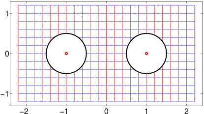
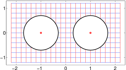
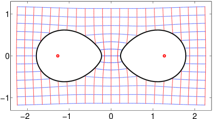
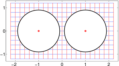
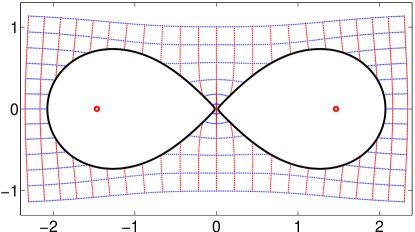
Figure 2: Original domains for Example 6.1 (left) and corresponding lemniscatic domains (right) obtained with $n=256$ and for $r=0.5$ (top), $r=0.7$ (middle), and $r=0.9$ (bottom).

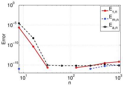
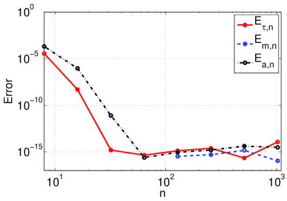
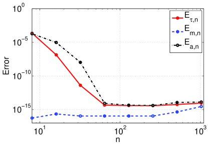
Figure 3: Errors $E_{a,n}$, $E_{m,n}$, and $E_{\tau,n}$ obtained with $n$ nodes and for $r=0.5$ (top left), $r=0.7$ (top right), and $r=0.9$ (bottom) in Example 6.1. Missing dots indicate that the error is zero.

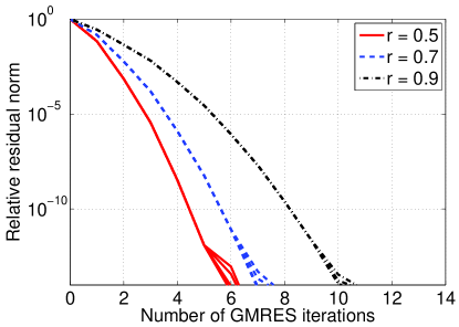
Figure 4: Relative residual norms of the GMRES method for different values of $r$ and $n$ in Example 6.1.

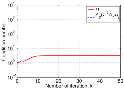
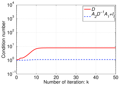
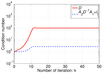
Figure 5: 2-norm condition numbers of $D$ and $A_{2}D^{-1}A_{1}+I_{\ell}$ obtained with $n=256$ and for $r=0.5$ (top left), $r=0.7$ (top right), and $r=0.9$ (bottom) in Example 6.1.

Figure 6: $\|{\bf z}^{k+1}-{\bf z}^{k}\|_{\infty}$ in the Newton iteration obtained with $n=256$ and for $r=0.5$, $r=0.7$, and $r=0.9$ in Example 6.1.

Example 6.2.

We consider the unbounded domain $\mathcal{K}$ exterior to seven nonconvex and complicated but smooth curves as shown in Figure 7. These curves are parametrized (from left to right) by

$$\eta_{j}(t)=r_{j}(t)\,e^{-\mathrm{i}t},\quad 0\leq t\leq 2\pi,\quad j=1,2,\ldots,7,$$

where

$$r_{1}(t) =1.25+0.50\sin(4t)+0.30\cos(t),$$

$$r_{2}(t) =1.25+0.40\sin(2t)+0.20\cos(3t),$$

$$r_{3}(t) =0.75+0.25e^{\cos(t)}\cos^{2}(3t)+0.50e^{\sin(t)}\sin^{2}(2t),$$

$$r_{4}(t) =e^{\cos(t)}\cos^{2}(2t)+e^{\sin(t)}\sin^{2}(2t),$$

$$r_{5}(t) =0.75+0.25e^{\cos(t)}\cos^{2}(2t)+0.50e^{\sin(t)}\sin^{2}(3t),$$

$$r_{6}(t) =1.25+0.40\sin(4t)+0.20\cos(3t),$$

$$r_{7}(t) =1.25+0.50\sin(3t)+0.30\cos(t).$$

The computed lemniscatic domain obtained with $n=256$ is shown on the bottom of Figure 7. The GMRES method for the seven linear algebraic systems required $36$ iteration steps to attain a residual norm smaller than $10^{-14}$. Figure 8 shows the 2-norm condition numbers of the matrices $D$ and $A_{2}D^{-1}A_{1}+I_{\ell}$ as well as the norms $\|{\bf z}^{k+1}-{\bf z}^{k}\|_{\infty}$ in the Newton iteration.

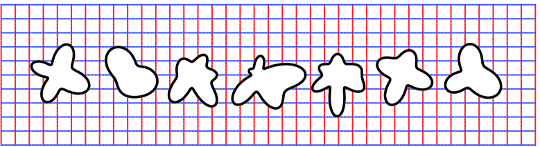
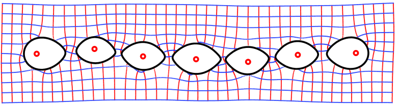
Figure 7: Original domain for Example 6.2 (top) and corresponding lemniscatic domain (bottom) obtained with $n=256$.

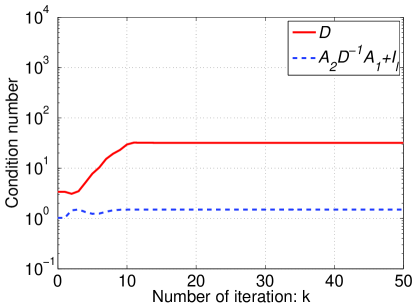
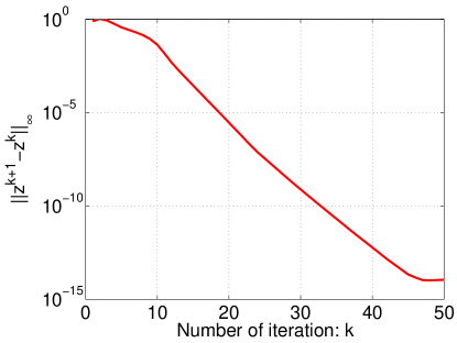
Figure 8: 2-norm condition numbers of $D$ and $A_{2}D^{-1}A_{1}+I_{\ell}$ (left) and norms $\|{\bf z}^{k+1}-{\bf z}^{k}\|_{\infty}$ (right) in Example 6.2.

Example 6.3.

In this example we demonstrate that our method also works for domains with high connectivity. We consider the unbounded domain $\mathcal{K}$ exterior to 64 circles as shown on the left of Figure 9. The domain $\mathcal{K}$ is symmetric with respect to both the real and the imaginary axis. Since the computed conformal map is normalized as in (3) the lemniscatic domain $\mathcal{L}$ has the same symmetry properties; see [42, Lemma 2.2]. The computed lemniscatic domain obtained with $n=256$ is shown on the right of that figure. The GMRES method for the 64 linear algebraic systems required between 14 and 18 iteration steps to attain a residual norm smaller than $2\cdot 10^{-14}$. Figure 10 shows the 2-norm condition numbers of $D$ and $A_{2}D^{-1}A_{1}+I_{\ell}$ as well as the norms $\|{\bf z}^{k+1}-{\bf z}^{k}\|_{\infty}$ in the Newton iteration.

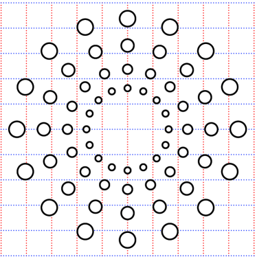
Figure 9: Original domain for Example 6.3 (left) and the corresponding lemniscatic domain (right) obtained with $n=256$.

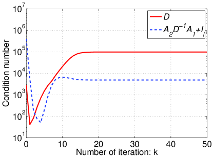
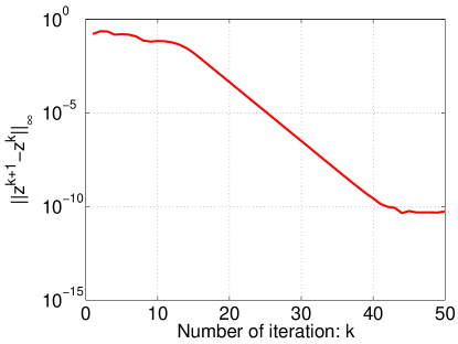
Figure 10: 2-norm condition numbers of $D$ and $A_{2}D^{-1}A_{1}+I_{\ell}$ (left) and the norms $\|{\bf z}^{k+1}-{\bf z}^{k}\|_{\infty}$ (right) in Example 6.3.

Example 6.4.

As indicated in Section 5.1, our method can also be used when the boundary components of $\mathcal{K}$ are only piecewise smooth Jordan curves. As an example we consider the unbounded domain $\mathcal{K}$ exterior to four squares as shown on the left of Figure 11. The computed lemniscatic domain obtained with $n=1024$ is shown on the right of that figure. The GMRES method for the four linear algebraic systems required 26 iteration steps to attain a residual norm smaller than $10^{-14}$. Figure 12 shows the 2-norm condition numbers of $D$ and $A_{2}D^{-1}A_{1}+I_{\ell}$ as well as the norms $\|{\bf z}^{k+1}-{\bf z}^{k}\|_{\infty}$ in the Newton iteration.

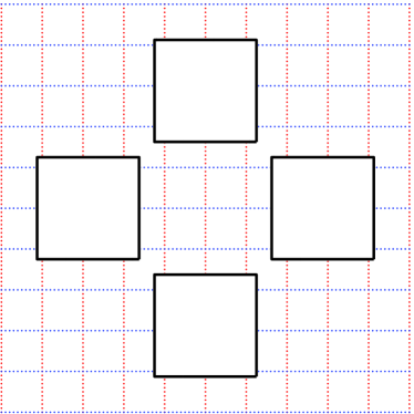
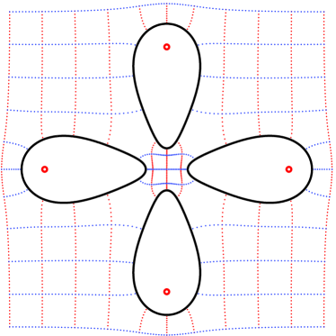
Figure 11: Original domain for Example 6.4 (left) and corresponding lemniscatic domain (right) obtained with $n=1024$.

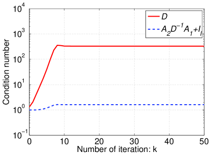
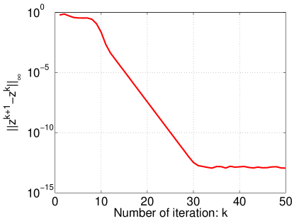
Figure 12: 2-norm condition numbers of $D$ and $A_{2}D^{-1}A_{1}+I_{\ell}$ (left) and the norms $\|{\bf z}^{k+1}-{\bf z}^{k}\|_{\infty}$ (right) in Example 6.4.

Example 6.5.

In this example we consider the unbounded domain $\mathcal{K}$ exterior to three non-convex sets as shown on the left of Figure 1. The three sets are of the form introduced in [22]. The boundary curves are analytic and an analytic parameterization is known as well. The corresponding lemniscatic domain obtained with $n=1024$ nodes per boundary component is shown on the right of Figure 1. The GMRES method for the three linear algebraic systems required between $32$ and $34$ iteration steps to attain a residual norm smaller than $10^{-14}$. Figure 13 shows the 2-norm condition numbers of $D$ and $A_{2}D^{-1}A_{1}+I_{\ell}$ as well as the norms $\|{\bf z}^{k+1}-{\bf z}^{k}\|_{\infty}$ in the Newton iteration.

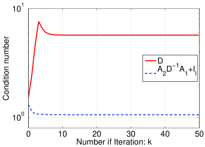
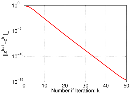
Figure 13: 2-norm condition numbers of $D$ and $A_{2}D^{-1}A_{1}+I_{\ell}$ (left) and the norms $\|{\bf z}^{k+1}-{\bf z}^{k}\|_{\infty}$ (right) in Example 6.5.

7 Concluding remarks

In this article we derived a method that numerically computes the conformal map from a given domain onto a lemniscatic domain. The method relies on solving a boundary integral equation with the Neumann kernel. It takes as input a parameterization of the boundary of the original domain and yields the parameters of the lemniscatic domain and the boundary values of the conformal map. Using the numerically computed conformal map $\Phi:\mathcal{K}\to\mathcal{L}$ it is in particular possible to compute the Faber–Walsh polynomials associated with the compact set $\widehat{\mathbb{C}}\setminus\mathcal{K}$. The first numerical examples for such a computation are given in the paper [43].

The transfinite diameter (or logarithmic capacity) of the set $\widehat{\mathbb{C}}\setminus\mathcal{K}$ is one of the parameters in its corresponding lemniscatic domain $\mathcal{L}$; see Theorem 2.1. This parameter is computed in the first step of the algorithm proposed in this paper; see Section 5.1. Since computing the transfinite diameter of compact sets is an interesting problem in its own right, we have derived a numerical method for this task, which is based on the method of Section 5.1, in our paper [27].

Let us point out a few open questions. As discussed in Section 5.1 and demonstrated numerically in Section 6, the GMRES method converges very fast when solving the discretized boundary integral equation with the Neumann kernel. A rigorous analysis of this effect is subject to further work. Further, it would be interesting to analyze how the accuracy of the solution of the linear algebraic systems (solved with GMRES) affects the accuracy of the computed conformal map and of the parameters of the lemniscatic domain. Finally, a “black box” starting point for the Newton iteration for solving the non-linear system (30) would be of interest.

Acknowledgements

We thank Robert Luce for helpful discussions on Cauchy matrices and the solution of the systems (35)–(36). We also thank Elias Wegert for suggesting our collaboration. We further thank the anonymous referees for helpful comments.

References

- [1] V. V. Andreev and T. H. McNicholl, Computing conformal maps of finitely connected domains onto canonical slit domains, Theory Comput. Syst., 50 (2012), pp. 354–369.
- [2] K. E. Atkinson, The numerical solution of integral equations of the second kind, vol. 4 of Cambridge Monographs on Applied and Computational Mathematics, Cambridge University Press, Cambridge, 1997.
- [3] A. P. Austin, P. Kravanja, and L. N. Trefethen, Numerical algorithms based on analytic function values at roots of unity, SIAM J. Numer. Anal., 52 (2014), pp. 1795–1821.
- [4] D. Crowdy, The Schwarz-Christoffel mapping to bounded multiply connected polygonal domains, Proc. R. Soc. Lond. Ser. A Math. Phys. Eng. Sci., 461 (2005), pp. 2653–2678.
- [5] , Schwarz-Christoffel mappings to unbounded multiply connected polygonal regions, Math. Proc. Cambridge Philos. Soc., 142 (2007), pp. 319–339.
- [6] D. Crowdy and J. Marshall, Conformal mappings between canonical multiply connected domains, Comput. Methods Funct. Theory, 6 (2006), pp. 59–76.
- [7] T. K. DeLillo, Schwarz-Christoffel mapping of bounded, multiply connected domains, Comput. Methods Funct. Theory, 6 (2006), pp. 275–300.
- [8] T. K. DeLillo, T. A. Driscoll, A. R. Elcrat, and J. A. Pfaltzgraff, Computation of multiply connected Schwarz-Christoffel maps for exterior domains, Comput. Methods Funct. Theory, 6 (2006), pp. 301–315.
- [9] T. K. DeLillo, T. A. Driscoll, A. R. Elcrat, and J. A. Pfaltzgraff, Radial and circular slit maps of unbounded multiply connected circle domains, Proc. R. Soc. Lond. Ser. A Math. Phys. Eng. Sci., 464 (2008), pp. 1719–1737.
- [10] T. K. DeLillo, A. R. Elcrat, E. H. Kropf, and J. A. Pfaltzgraff, Efficient calculation of Schwarz-Christoffel transformations for multiply connected domains using Laurent series, Comput. Methods Funct. Theory, 13 (2013), pp. 307–336.
- [11] T. K. DeLillo, A. R. Elcrat, and J. A. Pfaltzgraff, Schwarz-Christoffel mapping of multiply connected domains, J. Anal. Math., 94 (2004), pp. 17–47.
- [12] T. K. Delillo and E. H. Kropf, Numerical computation of the Schwarz-Christoffel transformation for multiply connected domains, SIAM J. Sci. Comput., 33 (2011), pp. 1369–1394.
- [13] A. Greenbaum, L. Greengard, and G. B. McFadden, Laplace’s equation and the Dirichlet-Neumann map in multiply connected domains, J. Comput. Phys., 105 (1993), pp. 267–278.
- [14] L. Greengard and Z. Gimbutas, FMMLIB2D: A MATLAB toolbox for fast multipole method in two dimensions, Version 1.2, http://www.cims.nyu.edu/cmcl/fmm2dlib/fmm2dlib.html, 2012.
- [15] L. Greengard and V. Rokhlin, A fast algorithm for particle simulations, J. Comput. Phys., 73 (1987), pp. 325–348.
- [16] H. Grunsky, Über konforme Abbildungen, die gewisse Gebietsfunktionen in elementare Funktionen transformieren. I, Math. Z., 67 (1957), pp. 129–132.
- [17] , Über konforme Abbildungen, die gewisse Gebietsfunktionen in elementare Funktionen transformieren. II, Math. Z., 67 (1957), pp. 223–228.
- [18] J. Helsing and R. Ojala, On the evaluation of layer potentials close to their sources, J. Comput. Phys., 227 (2008), pp. 2899–2921.
- [19] P. Henrici, Applied and computational complex analysis. Vol. 3, Pure and Applied Mathematics (New York), John Wiley & Sons, Inc., New York, 1986.
- [20] J. A. Jenkins, On a canonical conformal mapping of J. L. Walsh, Trans. Amer. Math. Soc., 88 (1958), pp. 207–213.
- [21] W. Kaplan, Introduction to analytic functions, Addison-Wesley Publishing Co., Reading, Mass.-London-Don Mills, Ont., 1966.
- [22] T. Koch and J. Liesen, The conformal “bratwurst” maps and associated Faber polynomials, Numer. Math., 86 (2000), pp. 173–191.
- [23] P. Koebe, Abhandlungen zur Theorie der konformen Abbildung, IV. Abbildung mehrfach zusammenhängender schlichter Bereiche auf Schlitzbereiche, Acta Math., 41 (1916), pp. 305–344.
- [24] R. Kress, A Nyström method for boundary integral equations in domains with corners, Numer. Math., 58 (1990), pp. 145–161.
- [25] , Linear integral equations, vol. 82 of Applied Mathematical Sciences, Springer, New York, third ed., 2014.
- [26] H. J. Landau, On canonical conformal maps of multiply connected domains, Trans. Amer. Math. Soc., 99 (1961), pp. 1–20.
- [27] J. Liesen, O. Sète, and M. M. S. Nasser, Computing the logarithmic capacity of compact sets via conformal mapping, arXiv:1507.05793, (2015).
- [28] W. Luo, J. Dai, X. Gu, and S.-T. Yau, Numerical conformal mapping of multiply connected domains to regions with circular boundaries, J. Comput. Appl. Math., 233 (2010), pp. 2940–2947.
- [29] N. I. Muskhelishvili, Singular integral equations, Noordhoff International Publishing, Leyden, 1977.
- [30] M. M. S. Nasser, A boundary integral equation for conformal mapping of bounded multiply connected regions, Comput. Methods Funct. Theory, 9 (2009), pp. 127–143.
- [31] , Numerical conformal mapping via a boundary integral equation with the generalized Neumann kernel, SIAM J. Sci. Comput., 31 (2009), pp. 1695–1715.
- [32] , Numerical conformal mapping of multiply connected regions onto the second, third and fourth categories of Koebe’s canonical slit domains, J. Math. Anal. Appl., 382 (2011), pp. 47–56.
- [33] , Numerical conformal mapping of multiply connected regions onto the fifth category of Koebe’s canonical slit regions, J. Math. Anal. Appl., 398 (2013), pp. 729–743.
- [34] , Fast computation of the circular map, Comput. Methods Funct. Theory, 15 (2015), pp. 187–223.
- [35] , Fast solution of boundary integral equations with the generalized Neumann kernel, Electron. Trans. Numer. Anal., 44 (2015), pp. 189–229.
- [36] M. M. S. Nasser and F. A. A. Al-Shihri, A fast boundary integral equation method for conformal mapping of multiply connected regions, SIAM J. Sci. Comput., 35 (2013), pp. A1736–A1760.
- [37] M. M. S. Nasser, A. H. M. Murid, M. Ismail, and E. M. A. Alejaily, Boundary integral equations with the generalized Neumann kernel for Laplace’s equation in multiply connected regions, Appl. Math. Comput., 217 (2011), pp. 4710–4727.
- [38] M. M. S. Nasser, T. Sakajo, A. H. M. Murid, and L. Wei, A fast computational method for potential flows in multiply connected coastal domains, Jpn. J. Ind. Appl. Math., 32 (2015), pp. 205–236.
- [39] Z. Nehari, Conformal mapping, McGraw-Hill Book Co., Inc., New York, Toronto, London, 1952.
- [40] A. Rathsfeld, Iterative solution of linear systems arising from the Nyström method for the double-layer potential equation over curves with corners, Math. Methods Appl. Sci., 16 (1993), pp. 443–455.
- [41] Y. Saad and M. H. Schultz, GMRES: a generalized minimal residual algorithm for solving nonsymmetric linear systems, SIAM J. Sci. Statist. Comput., 7 (1986), pp. 856–869.
- [42] O. Sète and J. Liesen, On conformal maps from multiply connected domains onto lemniscatic domains, arXiv:1501.01812, accepted for publication in Electron. Trans. Numer. Anal., (2015).
- [43] , Properties and examples of Faber–Walsh polynomials, arXiv:1502.07633, (2015).
- [44] J. L. Walsh, On the conformal mapping of multiply connected regions, Trans. Amer. Math. Soc., 82 (1956), pp. 128–146.
- [45] , A generalization of Faber’s polynomials, Math. Ann., 136 (1958), pp. 23–33.
- [46] , Interpolation and approximation by rational functions in the complex domain, Fifth edition. American Mathematical Society Colloquium Publications, Vol. XX, American Mathematical Society, Providence, R.I., 1969.
- [47] R. Wegmann, Methods for numerical conformal mapping, in Handbook of complex analysis: geometric function theory. Vol. 2, Elsevier, Amsterdam, 2005, pp. 351–477.
- [48] R. Wegmann and M. M. S. Nasser, The Riemann-Hilbert problem and the generalized Neumann kernel on multiply connected regions, J. Comput. Appl. Math., 214 (2008), pp. 36–57.
- [49] A. Yunus, A. Murid, and M. Nasser, Numerical conformal mapping and its inverse of unbounded multiply connected regions onto logarithmic spiral slit regions and rectilinear slit regions, Proc. R. Soc. A., 470 (2014), p. Article No. 20130514.