A Hierarchical Framework for State-Space Matrix Inference and Clustering

Abstract

In recent years, a large number of genomic and epigenomic studies have been focusing on the integrative analysis of multiple experimental datasets measured over a large number of observational units. The objectives of such studies include not only inferring a hidden state of activity for each unit over individual experiments, but also detecting highly associated clusters of units based on their inferred states. Although there are a number of methods tailored for specific datasets, there is currently no state-of-the-art modeling framework for this general class of problems. In this paper, we develop the MBASIC (Matrix Based Analysis for State-space Inference and Clustering) framework. MBASIC consists of two parts: state-space mapping and state-space clustering. In state-space mapping, it maps observations onto a finite state-space, representing the activation states of units across conditions. In state-space clustering, MBASIC incorporates a finite mixture model to cluster the units based on their inferred state-space profiles across all conditions. Both the state-space mapping and clustering can be simultaneously estimated through an Expectation-Maximization algorithm. MBASIC flexibly adapts to a large number of parametric distributions for the observed data, as well as the heterogeneity in replicate experiments. It allows for imposing structural assumptions on each cluster, and enables model selection using information criterion. In our data-driven simulation studies, MBASIC showed significant accuracy in recovering both the underlying state-space variables and clustering structures. We applied MBASIC to two genome research problems using large numbers of datasets from the ENCODE project. The first application grouped genes based on transcription factor occupancy profiles of their promoter regions in two different cell types. The second application focused on identifying groups of loci that are similar to a GATA2 binding site that is functional at its endogenous locus by utilizing transcription factor occupancy data and illustrated applicability of MBASIC in a wide variety of problems. In both studies, MBASIC showed higher levels of raw data fidelity than analyzing these data with a two-step approach using ENCODE results on transcription factor occupancy data.

¹ Department of Statistics, University of Wisconsin, Madison, WI, U.S.A.

² Department of Biostatistics and Medical Informatics, University of Wisconsin, Madison, WI, U.S.A.

³ Department of Cell and Regenerative Biology, University of Wisconsin, Madison, WI, U.S.A.

1 Introduction

The flow of genetic information through DNA transcription and RNA translation is a highly regulated process. The underlying mechanisms of regulation by both genomic and epigenomic factors are central targets in large numbers of genomic and epigenomic studies. This paper is motivated by a number of such studies that aim to elucidate genomic regulatory mechanisms across multiple biological conditions. Experiments that investigate such processes produce a plethora of data types. For example, relevant to DNA transcription is transcription factor occupancy data that quantify which regions of DNA are occupied by DNA binding proteins that can enhance or reduce gene expression. Histone modification data map covalent post-translational modifications to histone proteins, core proteins that make up the nucleosome structure of DNA. Such modifications impact DNA transcription by altering chromatin structure.

Computational and statistical analysis of these data often involve identifying genomic loci that show significant signal, i.e., enrichment, compared to background noise in the experimental measurements, with the operating principle that multiple loci might exhibit similar signal profile over different biological conditions.

Improvements in the next-generation sequencing technology further accelerated rapid generation of these types of data. In return, the vast availability of such data has revolutionized the scope of genome regulation studies. Previous analyses had been restricted to detecting regions of genome that were associated with one particular factor in one single organism. Many recent studies focus on detecting more complex functional patterns that integrate data from multiple organisms under multiple conditions. Namely, the associations between DNA elements and how they change across biological and/or experimental conditions have been the focus of many integrative modeling approaches. Examples of these studies include:

Differential binding analysis among multiple ChIP-seq data.

One of the key mechanisms of gene expression regulation is through differential activities of transcription factors and epigenetic modifications. Currently, chromatin immunoprecipitation followed by high throughput sequencing (ChIP-seq) is the state-of-the-art method for genome-wide profiling of protein-DNA interactions. Such two key interactions are DNA occupancy by transcription factors and histone modifications. Most transcription factors, i.e., DNA binding proteins, recognize DNA in a sequence specific manner and promote or represses gene expression. Similarly, histone modifications can induce diverse biological consequences such as transcriptional activation/deactivation. The study of gene regulation often involves comparing transcription factor occupancy and histone modifications across multiple biological conditions. Such conditions can be different treatment levels, time points of measurements, or different dosage levels (Liang and Keleş, 2012; Anders and Huber, 2010; Ji et al., 2013; Wei et al., 2015).

Transcription factor regulatory network analysis.

The combinatorial nature of transcription factor regulation underlies the large diversity observed in eukaryotic gene control. This largely motivates construction of regulatory networks that model gene expression as a combinatorial function of regulatory interactions between DNA and different transcription factors. The large-scale data from the ENCODE project (The ENCODE Project Consortium, 2012) now enable joint analyses of over one hundred human transcription factors across multiple cell types. Such analyses are posed to reveal a great amount of information about co-association patterns between different TFs, hierarchical network organizations, and systems-level integration of complex cellular signals (Neph1 et al., 2012; Gerstein et al., 2012; Cheng et al., 2011; Zeng et al., 2013). While the large number of TFs makes it computationally formidable to exhaust all possible combinatorial associations for such analyses, it is important to detect the most significant combinatorial patterns that preserve global regulatory dynamics.

Comparative functional genomic studies across different species.

Functional genomics analysis compares gene expressions or TF occupancy profiles between multiple species. The main task is to identify divergent and conserved functional modules that are central to evolutionary relationships (e.g., Kunarso et al. (2010), Schmidt et al. (2010)). Existing methods, that build on hidden Markov models (Roy et al., 2013) or biclustering (Waltman et al., 2010), implicitly assume that the functional modules should at least have similar signal profiles (i.e., expression, occupancy) among some subsets of the species under consideration. For these analyses, it is also important to identify functional modules that are fully divergent across species. These regions play an equally important role in understanding connectivity among species over the evolutionary history.

Although the types of data for these different studies vary, the underlying statistical principles are largely shared. Therefore, we propose a unified framework for the analysis of such data by formalizing the shared aspects. We formulate the underlying statistical problem as follows. Suppose a dataset $\{Y_{ik}\}$ is collected over a set of observational units (e.g., loci in genomic experiments) $i=1,2,\cdots,I$ under conditions $k=1,2,\cdots,K$. Inferring the association patterns within a single experiment involves mapping the corresponding set of observations $\{Y_{ik}:i=1,2,\cdots,I\}$ to a finite discrete state-space, $\mathscr{S}=\{1,2,\cdots,S\}$. This space contains different levels of association (e.g., enrichment/non-enrichment indicating the status of occupancy in ChIP-seq experiments, expressed/not expressed in RNA-seq gene expression experiments). This falls under the classical finite-mixture modeling framework, where a latent state variable $\theta_{ik}\in\mathscr{S}$ is inferred for each observational unit $Y_{ik}$. A higher level of modeling on the matrix $\Theta=(\theta_{ik})_{1\leq i\leq I,1\leq k\leq K}$ is required for integrating the association patterns under different conditions. We call this matrix the state-space matrix since it describes the latent states of individual observations.

We propose the following framework to model the state-space matrix $\Theta$. We assume that rows of $\Theta$ can be partitioned into $J+1$ subsets: $\{1,\cdots,I\}=\mathscr{C}_{0}\cup\mathscr{C}_{1}\cup\cdots\cup\mathscr{C}_{J}$. Rows of $\Theta$ within partition $\mathscr{C}_{j}$, $j\geq 1$, are generated by the same distribution parametrized by $w_{j\cdot}=(w_{jk})_{1\leq k\leq K}$:

$$\theta_{ik}\sim g(\cdot|w_{jk}),\quad i\in\mathscr{C}_{j},$$

while the rows of $\mathscr{C}_{0}$, which denotes the group of ”singleton” units, i.e., units that do not cluster in any of the $J$ groups, are generated by row specific distributions. The goal of this model is thus to estimate a partitioning that best characterizes the row associations of state-space matrix $\Theta$.

We refer to the proposed framework as Matrix Based Analysis for State-space Inference and Clustering (MBASIC). MBASIC is related to classical factor analysis which considers the problem of projecting one dimension (either row or column) of large noisy matrices into low-dimensional spaces. MBASIC has two distinguished features compared to the existing literature in these areas. First, MBASIC deals with matrices with discrete entries, while most existing methods are designed for matrices on continuous scales. Second, MBASIC estimates the low-dimensional projection by grouping the rows of the original matrix in contrast to the Principle Component Analysis (PCA) approaches which form linear combinations of the rows (e.g., Ji et al. (2013), Lee et al. (2010)). This is motivated by the following arguments:

1. In MBASIC, each factor estimate $w_{j\cdot}$ characterizes the commonality of a group of rows and is easily interpretable in practice. Such interpretability can further be enhanced by imposing structural restrictions on the $w_{j\cdot}$ vector for practical purposes. Examples of such constraints are described in Section 3.3;

2. PCA for high dimensional matrices are often accompanied by regularization techniques, which are computationally prohibitive for many epigenetic datasets. In contrast, clustering the matrix rows can be implemented very efficiently and in a straightforward manner.

The hierarchical structure of MBASIC is similar to two other recently proposed statistical models: iASeq (Wei et al., 2012) and Cormotif (Wei et al., 2015). Both these models incorporate a state-space clustering structure similar to MBASIC. MBASIC extends these models in several critically essential directions. First, MBASIC is developed for general purposes and can be easily implemented for a wide range of parametric distributions, while Cormotif and iASeq operate with specific distributions targeting the problems of differential expression and allele-specific binding. Second, neither of these models include a group of singletons with idiosyncratic state-space profiles. When we are agnostic about the “true” clustering structure in applications, separating the singletons can reduce their influence on the estimation of clustering parameters. Third, both iASeq and Cormotif separate estimation for the distributional parameters from the clustering structure, while MBASIC jointly fits all model parameters. A limiting assumption of MBASIC compared to these models is that MBASIC does not allow the distributional parameters within the same state to be heterogeneous. However, a pre-processing step that accounts for the the heterogeneity can overcome such a limitation. We evaluate and discuss all of these features with extensive simulation studies in this paper.

This paper is organized as follows. We start with a formal description of MBASIC in Section 2, followed by model estimation and selection methods in Section 3. We also investigate general features of MBASIC compared to iASeq and Cormotif with extensive simulations in this section. Section 4 presents results from several real data examples. Mathematical details of the algorithm are included in Appendix A.1.

2 The Hierarchical Mixture Model Framework

Consider a dataset with observations from $I$ different observational units under $K$ different conditions. For each condition $k\in\{1,2,\cdots,K\}$, there are $n_{k}$ replicate experiments, indexed by $l=1,2,\cdots,n_{k}$. We use $Y_{ikl}$ to denote the observation for the $l$-th replicate of unit $i$ under condition $k$. For each condition $k$ at unit $i$, there exists a hidden state variable $\theta_{ik}\in\mathscr{S}=\{1,2,\cdots,S\}$. The MBASIC model consists of the following components:

1. State-space Mapping:

   $$Y_{ikl}|\theta_{ik}=s{\buildrel\rm ind.\over{\sim}}f_{s}(\cdot|\mu_{kls},\sigma_{kls},\gamma_{ikls}).$$ (1)

2. State-space Clustering: $\theta_{ik}$’s are independently sampled from $\mathscr{S}$ with the sampling probability:

   $$P(\theta_{ik}=s)=\zeta p_{is}+(1-\zeta)\sum_{j=1}^{J}\pi_{j}w_{jks}.$$ (2)

In (1), $\mu_{kls}$ and $\sigma_{kls}$ are the parameters related to the mean and dispersion for the $s$-th state for replicate $l$ under condition $k$, and $\gamma_{ikls}$ is the covariate encoding known information for unit $i$. In (2), $p_{is}$, $\zeta$, $\pi_{j}$, and $w_{jks}$ are additional non-negative parameters subject to restrictions:

$$\quad 0\leq\zeta\leq 1;\quad\sum_{j=1}^{J}\pi_{j}=1;\quad\sum_{s=1}^{S}w_{jks}=1,\forall j,k;\quad\sum_{s=1}^{S}p_{is}=1,\forall i.$$

We further discuss these parameters in Section 2.2.

2.1 State-space Mapping

Equation 1 partitions observational units $i=1,\cdots,I$ into $S$ subsets according to their hidden states. Within the same replicate, data from the same hidden state follow the same distribution $f_{s}(\cdot|\mu_{kls},\sigma_{kls},\gamma_{ikls})$. MBASIC assumes that the hidden states $\theta_{ik}$’s are independent of the replicate index $l$, which means all replicates under the same condition have the same set of hidden states. However, distributional parameters for a given state can be different among replicates. Such a setting allows for the flexibility of modeling the heterogeneity in replicate experiments.

The density function $f$ can be from an arbitrary parametric distribution. We consider three fundamental families of distributions commonly used for genomic data analysis:

• Log-normal Distribution. $LN(\mu_{kls}\gamma_{ikls},\sigma_{kls})$ with a density function:

  $$f_{s}(y|\mu_{kls},\sigma_{kls},\gamma_{ikls})=\frac{1}{\sqrt{2\pi}\sigma_{kls}}\exp\left\{-\frac{(\log(y+1)-\mu_{kls}\gamma_{ikls})^{2}}{2\sigma_{kls}^{2}}\right\}.$$ (3)

• Negative Binomial Distribution. $NB(\mu_{kls}\gamma_{ikls},\sigma_{kls})$ with a density function:

  $$f_{s}(y|\mu_{kls},\sigma_{kls},\gamma_{ikls})=\frac{\Gamma(y+\sigma_{kls})}{\Gamma(\sigma_{kls})\Gamma(y)}\frac{(\mu_{kls}\gamma_{ikls})^{y}\sigma_{kls}^{\sigma_{kls}}}{(\mu_{kls}\gamma_{ikls}+\sigma_{kls})^{y+\sigma_{kls}}}.$$ (4)

• Binomial Distribution. $Binom(\gamma_{ikls},\mu_{kls})$ with a density function:

  $$f_{s}(y|\mu_{kls},\gamma_{ikls})={\gamma_{ikls}\choose y}\mu_{kls}^{y}(1-\mu_{kls})^{\gamma_{ikls}-y}.$$ (5)

In these three examples, $\gamma_{ikls}$ represents the known heterogeneity across loci whereas $\mu_{kls}$ and $\sigma_{kls}$ are unknown parameters. For example, when using Eqn. (3) or (4) in a ChIP-seq analysis with $S=2$ states, we can estimate $\gamma_{ikl1}$ using data from the control samples so that the ChIP sample read counts in the background state scale with the control sample data (e.g., as in Zuo and Keleş (2013)), and assume $\gamma_{ikl2}=1$ for the enriched states. Eqn. (5) can be used to analyze allele-specific binding data, where $\gamma_{ikls}$ is the total read counts from both paternal and maternal alleles and is constant across $s$. Application with the binomial distribution also requires that $\mu_{kls}\sum_{i=1}^{I}\gamma_{ikls}$, $\forall k,l$, is strictly increasing in $s$ for model identification.

The MBASIC can be easily extended to other classes of parametric distributions and estimation for these distributions follows the same Expectation-Maximization skeleton. While Section 3 relies on these three distributions to describe the model and the estimation algorithms, the second real data example in Section 4 utilizes a more complex parametrization, which demonstrates the wide applicability of the MBASIC framework. Furthermore, we consider the following degenerate distribution:

$$f_{s}(y|\mu_{kls},\sigma_{kls},\gamma_{ikls})=I(y=s),$$ (6)

where I(.) denotes the indicator function. This degenerate form corresponds to the situation where the states, $\theta_{ik}$’s, are directly observed rather than inferred from $Y_{ikl}$’s. We utilize this parametrization for comparing MBASIC to alternative two-step analysis approaches in Section 3.5. Parameter estimation for this case follows a slightly modified procedure from the non-degenerate cases, which is described in Section 3.

2.2 State-space Clustering

Equation (2) models the distribution of $\theta_{ik}$ as a mixture of multiple distributions. To illustrate this model we introduce additional variables. The goal is to identify $J$ clusters from the set of observation units $1\leq i\leq I$. Let $b_{i}=I(\mbox{unit $i$ does not belong to any cluster})$ and $z_{ij}=I(\mbox{unit $i$ belongs to cluster $j$})$. The $b_{i}$ variables entertain the possibility that some observations are ”singletons”, i.e., they do not cluster with any other observational units. With these additional variables, the distribution in Equation (2) can be hierarchically decomposed as follows:

• $b_{i}{\buildrel\rm i.i.d.\over{\sim}}Bernoulli(\zeta)$;

• $(z_{i1},~{}z_{i2},\cdots,~{}z_{iJ}){\buildrel\rm i.i.d.\over{\sim}}MultiNom(1,(\pi_{1},~{}\pi_{2},\cdots,~{}\pi_{J}))$;

• Conditional on $b_{i}$ and $z_{ij}$, $\theta_{ik}$’s are independent samples from $\mathscr{S}$, with sampling probabilities $P(\theta_{ik}=s|b_{i}=1)=p_{is}$, $P(\theta_{ik}=s|b_{i}=0,z_{ij}=1)=w_{jks}$.

In this set up, although the singleton state-space probabilities $p_{is}$ are assumed to be constant across conditions, i.e., $P(\theta_{ik}=s)=p_{is}$, $\forall k$, this assumption is mildly restrictive since it accommodates $(P(\theta_{ik}=1,\cdots,P(\theta_{ik}=S))$ to follow an arbitrary prior distribution (e.g., $(P(\theta_{ik}=1,\cdots,P(\theta_{ik}=S))~{}\sim Dirichlet(\alpha,\cdots,\alpha),\forall k$) as long as it leads to the same marginal distribution for $\theta_{ik}$ for all $k$.

It is worth noting that this hierarchical structure essentially seeks a low-rank representation for the matrix $\Theta=(\theta_{ik})_{1\leq i\leq I,1\leq k\leq K}$. To illustrate this, we introduce additional matrices $\Theta_{s}=(I(\theta_{ik}=s))_{1\leq i\leq I,1\leq k\leq K}$, $W_{s}=(w_{jks})_{1\leq j\leq J,1\leq k\leq K}$, $Z=(z_{ij})_{1\leq i\leq I,1\leq j\leq J}$ and vectors $p_{s}=(p_{is})_{1\leq i\leq I}$, $B=(b_{i})_{1\leq i\leq I}$. Then, the conditional expectation of $\Theta_{s}$ is:

$$E(\Theta_{s}|Z,B)=(ZW_{s})\circ((1-B)1_{K}^{T})+(p_{s}\circ B)1_{K}^{T},$$ (7)

where “$\circ$” denotes the Hadamard product. We note that $E(\Theta_{s}|Z,B)$ is a matrix of rank $J+1$, which is usually much smaller than the dimension of the matrix $\Theta_{s}$. Similar models for low-rank representation of discrete matrices were considered in Lee et al. (2010), and turned out to be challenging both theoretically and computationally. The row-clustering structure for the matrices $E(\Theta_{s}|Z,B)$ in MBASIC is more restrictive than the general low-rank structure. Such additional restrictions not only reduce the difficulty in parameter estimation but also enable the flexibility in many useful ways. For example, while Lee et al. (2010) can only estimate one matrix at a time and thus is only applicable when $S=2$, MBASIC can be applied to arbitrary values of $S$.

3 Model Estimation and Selection

3.1 Likelihood Functions

In the MBASIC model, the likelihood function for both the observed random variables $Y_{ikl}$’s and the unobserved $\theta_{ik}$’s, $z_{ij}$’s, $b_{i}$’s, i.e., full data likelihood, is given by:

$$l (\mu,\sigma,\pi,p,\zeta,w;y,\theta,z,b)=$$ (8)

$$\prod_{i=1}^{I}\zeta^{b_{i}}(1-\zeta)^{1-b_{i}}\cdot\prod_{i=1}^{I}\prod_{k=1}^{K}\prod_{s=1}^{S}p_{is}^{I(\theta_{ik}=s)b_{i}}\cdot\prod_{i=1}^{I}\prod_{j=1}^{J}\pi_{j}^{z_{ij}}$$

$$\cdot \prod_{i=1}^{I}\prod_{k=1}^{K}\prod_{s=1}^{S}\left[\prod_{l=1}^{n_{k}}f_{s}(y_{ikl}|\mu_{kls},\sigma_{kls},\gamma_{ikls})\right]^{I(\theta_{ik}=s)}\cdot\prod_{i=1}^{I}\prod_{j=1}^{J}\prod_{k=1}^{K}\prod_{s=1}^{S}w_{jks}^{I(\theta_{ik}=s)(1-b_{i})z_{ij}}.$$

For non-degenerate distributions, we can show that the marginal likelihood is:

$$l(\mu,\sigma,\pi,p,\zeta,w;y)= \prod_{i=1}^{I}\left\{\zeta\prod_{k=1}^{K}\left[\sum_{s=1}^{S}p_{is}\prod_{l=1}^{n_{k}}f_{s}(y_{ikl}|\mu_{kls},\sigma_{kls},\gamma_{ikls})\right]\right.$$ (9)

$$+ \left.(1-\zeta)\sum_{j=1}^{J}\pi_{j}\prod_{k=1}^{K}\left[\sum_{s=1}^{S}w_{jks}\prod_{l=1}^{n_{k}}f_{s}(y_{ikl}|\mu_{kls},\sigma_{kls},\gamma_{ikls})\right]\right\}.$$

Equation (9) is easily interpretable. Conditional on $b_{i}$ and $z_{ij}$, the joint distribution for each $Y_{ikl},~{}1\leq l\leq n_{k}$ is a mixture of $S$ components, where the weight on the s-th component is either $p_{is}$ (when $b_{i}=1$) or $w_{jks}$ (when $b_{i}=0$ and $z_{ij}=1$). This yields the expressions in the square brackets. Integrating out $b_{i}$ and $z_{ij}$, the joint distribution for $Y_{ikl}$ of fixed $i$ is a mixture of $J+1$ components, with probability $\zeta$ of being a singleton and probability $(1-\zeta)\pi_{j}$ of belonging to cluster $j$.

For the degenerate case, by substituting (6) into (9), it can be shown that the marginal likelihood is:

$$l(\mu,\sigma,\pi,p,\zeta,w;\theta)=\prod_{i=1}^{I}\left\{\zeta\prod_{k=1}^{K}\prod_{s=1}^{S}p_{is}^{I(\theta_{ik}=s)}+(1-\zeta)\sum_{j=1}^{J}\pi_{j}\prod_{k=1}^{K}\prod_{s=1}^{S}w_{jks}^{I(\theta_{ik}=s)}\right\}.$$ (10)

3.2 An Expectation and Maximization (E-M) Algorithm

The hierarchical structure of MBASIC naturally fits in the Expectation-Maximization algorithm Dempster et al. (1977), which maximizes the marginal likelihood (equations (9) or (10)) by iteratively maximizing the complete data log-likelihood function. We let $\phi$ to denote a vector including all unknown parameters $\mu$, $\sigma$, $\pi$, $p$, $\zeta$, $w$, and $\hat{\phi}^{(t)}$ to denote the parameter estimates at the $t$-th iteration. The complete data log-likelihood function is:

$$Q(\phi|\hat{\phi}^{(t-1)})= \sum_{i=1}^{I}\sum_{k=1}^{K}\sum_{s=1}^{S}\left[\sum_{l=1}^{n_{k}}\log f_{s}(y_{ikl}|\mu_{kls},\sigma_{kls},\gamma_{ikls})\right]E[I(\theta_{ik}=s)|\hat{\phi}^{(t-1)}]$$ (11)

$$+ \sum_{i=1}^{I}\sum_{k=1}^{K}\sum_{s=1}^{S}\log p_{is}E[I(\theta_{ik}=s)b_{i}|\hat{\phi}^{(t-1)}]+\sum_{i=1}^{I}\sum_{j=1}^{J}\log\pi_{j}E[z_{ij}(1-b_{i})|\hat{\phi}^{(t-1)}]$$

$$+ \sum_{i=1}^{I}\{\log\zeta E[b_{i}|\hat{\phi}^{(t-1)}]+\log(1-\zeta)(1-E[b_{i}|\hat{\phi}^{(t-1)}])\}$$

$$+ \sum_{i=1}^{I}\sum_{k=1}^{K}\sum_{j=1}^{J}\sum_{s=1}^{S}E[I(\theta_{ik}=s)z_{ij}(1-b_{i})|\hat{\phi}^{(t-1)}]\log w_{jks}.$$

The E-M algorithm for MBASIC is outlined by Algorithm 1. E-step updates are listed in equations (12)-(15) and their derivations are provided in Appendix A.

Algorithm 1 Expectation-Maximization (EM)

  for $t=1,~{}2,\cdots$ until convergence do

     Expectation Step: Compute the conditional expectations $E[I(\theta_{ik}=s)|\hat{\phi}^{(t-1)}]$, $E[b_{i}|\hat{\phi}^{(t-1)}]$, $E[I(\theta_{ik}=s)b_{i}|\hat{\phi}^{(t-1)}]$, $E[z_{ij}(1-b_{i})|\hat{\phi}^{(t-1)}]$, $E[I(\theta_{ik}=s)z_{ij}(1-b_{i})|\hat{\phi}^{(t-1)}]$;

     Maximization Step: Update estimates for parameters $\mu_{kls}$, $\sigma_{kls}$, $\zeta$, $\pi_{j}$, $w_{jks}$, $p_{is}$ as maximizers for (11) .

  end for

$$E( b_{i}|\hat{\phi}^{(t-1)})=$$ (12)

$$\frac{\hat{\zeta}^{(t-1)}\prod_{k=1}^{K}\left(\sum_{s=1}^{S}\hat{f}_{iks}^{(t-1)}\hat{p}_{is}^{(t-1)}\right)}{(1-\hat{\zeta}^{(t-1)})\sum_{j=1}^{J}\hat{\pi}_{j}^{(t-1)}\prod_{k=1}^{K}\left(\sum_{s=1}^{S}\hat{f}_{iks}^{(t-1)}\hat{w}_{jks}^{(t-1)}\right)+\hat{\zeta}^{(t-1)}\prod_{k=1}^{K}\left(\sum_{s=1}^{S}\hat{f}_{iks}^{(t-1)}\hat{p}_{is}^{(t-1)}\right)},$$

$$E(z_{ij}(1-b_{i})|\hat{\phi}^{(t-1)})=\frac{\hat{\pi}_{j}^{(t-1)}\prod_{k=1}^{K}\left(\sum_{s=1}^{S}\hat{f}_{iks}^{(t-1)}\hat{w}_{jks}^{(t-1)}\right)}{\sum_{j=1}^{J}\hat{\pi}^{(t-1)}_{j}\prod_{k=1}^{K}\left(\sum_{s=1}^{S}\hat{f}_{iks}^{(t-1)}\hat{w}_{jks}^{(t-1)}\right)}[1-E(b_{i}|\hat{\phi}^{(t-1)})],$$ (13)

$$E(I(\theta_{ik}=s)z_{ij}(1-b_{i})|\hat{\phi}^{(t-1)})=$$ (14)

$$[1-E(b_{i}|\hat{\phi}^{(t-1)})]\frac{\hat{\pi}_{j}^{(t-1)}\prod_{k=1}^{K}\left(\sum_{s=1}^{S}\hat{f}_{iks}^{(t-1)}\hat{w}_{jks}^{(t-1)}\right)}{\sum_{j=1}^{J}\hat{\pi}_{j}^{(t-1)}\prod_{k=1}^{K}\left(\sum_{s=1}^{S}\hat{f}_{iks}^{(t-1)}\hat{w}_{jks}^{(t-1)}\right)}\cdot\frac{\hat{f}_{iks}^{(t-1)}\hat{w}_{jks}^{(t-1)}}{\sum_{s=1}^{S}\hat{f}_{iks}^{(t-1)}\hat{w}_{jks}^{(t-1)}},$$

$$E(I(\theta_{ik}=s)b_{i}|\hat{\phi}^{(t-1)})=E(b_{i}|\hat{\phi}^{(t-1)})\cdot\frac{\hat{f}_{iks}^{(t-1)}\hat{p}_{is}^{(t-1)}}{\sum_{s=1}^{S}\hat{f}_{iks}^{(t-1)}\hat{p}_{is}^{(t-1)}},$$ (15)

where $\hat{f}_{iks}^{(t-1)}=\prod_{l=1}^{n_{k}}f(y_{ikl}|\hat{\mu}_{kls}^{(t-1)},\hat{\sigma}_{kls}^{(t-1)},\gamma_{ikls})$. Given these results from the E-step, updates of $\zeta$, $\pi_{j}$, $w_{jks}$, $p_{is}$ in the M-step are straight forward as in equations (16), (17), (18), and (19).

$$\hat{\zeta}^{(t)} = \frac{\sum_{i=1}^{I}E[b_{i}|\hat{\phi}^{(t-1)}]}{I},$$ (16)

$$\hat{\pi}_{j}^{(t)} = \frac{\sum_{i=1}^{I}E[z_{ij}(1-b_{i})|\hat{\phi}^{(t-1)}]}{\sum_{i=1}^{I}\sum_{j=1}^{J}E[z_{ij}(1-b_{i})|\hat{\phi}^{(t-1)}]},$$ (17)

$$\hat{p}_{is}^{(t)} = \frac{\sum_{k=1}^{K}E[I(\theta_{ik}=s)b_{i}|\hat{\phi}^{(t-1)}]}{\sum_{s=1}^{S}\sum_{k=1}^{K}E[I(\theta_{ik}=s)b_{i}|\hat{\phi}^{(t-1)}]},$$ (18)

$$\hat{w}_{jks}^{(t)} = \frac{\sum_{i=1}^{I}E[I(\theta_{ik}=s)z_{ij}(1-b_{i})|\hat{\phi}^{(t-1)}]}{\sum_{s=1}^{S}\sum_{i=1}^{I}E[I(\theta_{ik}=s)z_{ij}(1-b_{i})|\hat{\phi}^{(t-1)}]}.$$ (19)

Updates for $\mu_{kls}$ and $\sigma_{kls}$ have to be treated according to the specific distributions. For the log-normal distributions (3), we have:

$$\quad\hat{\mu}_{kls}^{(t)} = \frac{\sum_{i=1}^{I}\log(y_{ikl}+1)P[\theta_{ik}=s|\hat{\phi}^{(t-1)}]}{\sum_{i=1}^{I}\gamma_{ikls}P[\theta_{ik}=s|\hat{\phi}^{(t-1)}]},$$ (20)

$$\quad\hat{\sigma}_{kls}^{(t)2} = \frac{\sum_{i=1}^{I}P[\theta_{ik}=s|\hat{\phi}^{(t-1)}][\log(y_{ikl}+1)-\hat{\mu}_{kls}^{(t)}\gamma_{ikls}]^{2}}{\sum_{i=1}^{I}P[\theta_{ik}=s|\hat{\phi}^{(t-1)}]}.$$ (21)

For the binomial distributions (5), we have:

$$\quad\hat{\mu}_{kls}^{(t)}=\frac{\sum_{i=1}^{I}y_{ikl}P[\theta_{ik}=s|\hat{\phi}^{(t-1)}]}{\sum_{i=1}^{I}\gamma_{ikls}P[\theta_{ik}=s|\hat{\phi}^{(t-1)}]}.$$ (22)

Closed form maximizers of $\mu$ and $\sigma$ do not exist for the negative binomial distribution (4). We adopt the method of moment estimates as in Kuan et al. (2011); Zuo and Keleş (2013), where the updated values $\hat{\mu}_{kls}^{(t)}$ and $\hat{\sigma}_{kls}^{(t)}$ are the solutions of the following equations:

$$\hat{\mu}_{kls}^{(t)}\sum_{i=1}^{I}\gamma_{ikls}P[\theta_{ik}=s|\hat{\phi}^{(t-1)}] = \sum_{i=1}^{I}y_{ikl}P[\theta_{ik}=s|\hat{\phi}^{(t-1)}],$$

$$\sum_{i=1}^{I}\left[\hat{\mu}_{kls}^{(t)2}\gamma_{ikls}^{2}\left(1+\frac{1}{\hat{\sigma}_{kls}^{(t)}}\right)+\hat{\mu}_{kls}^{(t)}\gamma_{ikls}\right]P[\theta_{ik}=s|\hat{\phi}^{(t-1)}] = \sum_{i=1}^{I}y_{ikl}^{2}P[\theta_{ik}=s|\hat{\phi}^{(t-1)}].$$

For the degenerate distributions as in (6), $\theta_{ik}$’s are directly observed. Therefore, the E-M algorithm for this case requires slight modifications: we skip the estimation for $E[I(\theta_{ik}=s)|\hat{\phi}^{(t-1)}]$ in the E-step and for $\mu$, $\sigma$ in the M-step.

3.3 Estimating Structured Clusters

In integrative functional genomics studies, the set of experimental conditions usually consists of interactions of multiple experimental factors; hence, it is often important to identify clusters, states of which are homogeneous across the levels of one or more factors. For example, in a typical transcription factor network analysis, experimental conditions include the combination of different cell types and TFs. It is often desirable to separate loci groups whose states are homogeneous within each cell type from those with cell type specific states for the purpose of cell type comparison. Depending on the cell types involved, such comparison can yield insights on cell development, pathology and/or cell-specific functions. We refer to clusters with homogeneous states within each cell type as TF-homogeneous. Another example is encountered in comparative functional genomics studies across different species, where experimental conditions range across both species and TFs. Clusters of loci, states of which are homogeneous across species conditional on each TF, constitute conserved functional modules. The TF-homogeneous clusters in this context represent the marginal effect of the species factor, and play a central role in understanding the evolutionary relationships.

To estimate a cluster with homogeneity for a particular experimental factor, MBASIC allows structural constraints on its state-space parameters. Recall that the parameters of cluster $j$ are represented by $w_{j.s}=(w_{j1s},w_{j2s},\cdots,w_{jKs})$. Marginalizing the effect of this factor, the $K$ experimental conditions can be partitioned into $M$ sets, $\{1,2,\cdots,K\}=T_{1}\cup T_{2}\cup\cdots\cup T_{M}$, where conditions within each set differ only in the levels of this factor. The parameters of this cluster satisfy the following constraints:

$$w_{jk_{1}s}=w_{jk_{2}s},\quad\mbox{if}\quad\exists~{}m\quad s.t.\quad k_{1},k_{2}\in T_{m}.$$ (23)

Cell Type Levels:	Gm12878			K562
TF Levels:	Atf3	Ctcf	Gata1	Atf3	Ctcf	Gata1
TF-homogeneous:	$w_{j1s}$	$w_{j2s}$	$w_{j3s}$	$w_{j4s}$	$w_{j5s}$	$w_{j6s}$
Cell Type-homogeneous:	$w_{j1s}$	$w_{j2s}$	$w_{j3s}$	$w_{j4s}$	$w_{j5s}$	$w_{j6s}$

Figure 1: A graphical description for a parametrization with structural constraints. Interactions of 2 cell types and 3 TFs result in six experimental conditions. Parameters with homogeneous values are shaded by the same color.

A pictorial depiction with six experimental conditions due to full interaction between 2 cell types and 3 TFs is depicted in Figure 1. Estimating structured clustering models follows the previous E-M algorithm with a modification in Equation (19). A constrained maximizer for $w_{jks}$ subject to constraint (23) is computed as:

$$\hat{w}_{jks}^{(t)}=\frac{\sum_{k^{\prime}:k^{\prime}\in T_{m}}\sum_{i=1}^{I}E[I(\theta_{ik^{\prime}}=s)z_{ij}(1-b_{i})|\hat{\phi}^{(t-1)}]}{\#\{T_{m}\}\sum_{s=1}^{S}\sum_{i=1}^{I}E[I(\theta_{ik}=s)z_{ij}(1-b_{i})|\hat{\phi}^{(t-1)}]},~{}~{}k\in T_{m}.$$

MBASIC requires that such structural constraints must be specified a priori and remain fixed during model fitting. MBASIC incorporates a model selection procedure to compare models with different hypothesized structural constraints and numbers of clusters. We next describe the details of this model selection procedure.

3.4 Model Selection

The MBASIC framework so far assumes that the total number of clusters $J$ is known a priori. In practice, models with varying values of $J$ need to be fitted independently and compared with each other according to some information criterion to determine the best value of $J$. Since the E-M algorithm aims to maximize the data likelihood function, AIC and BIC criteria can be utilized with MBASIC. The degrees of freedom for a model with $J$ clusters is $df=F_{1}S\sum_{k=1}^{K}n_{k}+(S-1)I+J+F_{2}$, where $F_{1}=2$ for distributions (3) and (4), $F_{1}=1$ for (5), and $F_{2}$ is the total number of free variables among $w_{jks}$’s. If there are no structured clusters, we have $F_{2}=JK(S-1)$.

When there is no prior information available, both the total number of clusters and the number of clusters following structural constraints have to be determined. This results in a prohibitively large number of candidate models, and computing the information criterion for each of them is not practical. In such cases we incorporate the following two-phase strategy to limit the number of candidate models:

1. Evaluate models with varying total number of clusters without any structural constraints. Select $J_{opt}$ according to the minimal AIC or BIC value.

2. Evaluate models with the fixed number of $J_{opt}$ clusters while varying the number of clusters following each structural constraint. Select the number of clusters following each structural constraint based on the minimal AIC or BIC value.

We acknowledge that the above two-step strategy is only a practical compromise to restrict the space of candidate models and does not guarantee finding the best model that globally minimizes the information criterion. However, we have conducted extensive simulation studies which illustrated that the proposed two-phase strategy performs well in a wide variety of settings.

3.5 Simulation Studies

Table 1: Design of the simulation studies. $S$: size of the state-space; $\zeta$: Proportion of singletons; $I$: number of units; $J$: number of clusters; $K$: number of experimental conditions.

Study	Distribution	$S$	$\zeta$	$I$	$(J,K)$	Model Selection
1	LN, NB, Bin	2, 3, 4	0, 0.1, 0.4	4000	(20, 30)	No
2	LN, NB, Bin	2	0.1, 0.4	4000	(20, 30)	Yes
3	iASeq	3	0, 0.1, 0.4	4000	(10, 20), (20, 30)	Yes
4	Cormotif	2	0	10,000	(4, 4), (5, 8), (5, 10)	Yes
5	Cormotif	2	0, 0.1, 0.4	4000	(10, 20)	Yes
6	LN	2	0, 0.33	4120, 4600, 6120	(8, 30)	Yes

We conducted 6 model-based simulation studies to investigate the performance of MBASIC in various settings as summarized in Table 1. Each simulation study has multiple settings that vary the distributional assumptions, size of the state-space ($S$), proportion of singletons ($\zeta$), number of units ($I$), number of clusters ($J$), and number of conditions ($K$). We provide the details of these simulation studies in Appendix B and highlight the overall conclusions in this section.

Data in Simulation Studies 1-2 were simulated according to MBASIC’s distributional assumptions. In Simulation Study 1, we emphasized two most important features of MBASIC: the joint estimation procedure of all model parameters and the inclusion of a singleton cluster. We derived six alternative algorithms (Table B.1) to benchmark MBASIC’s performance in various settings. Three of the algorithms (SE-HC, SE-MC, PE-MC) use two-stage procedures for model estimation, decoupling either the estimation of the state-space variables or the distributional parameters from the mixture modeling of clustering analysis. The other three algorithms are created as variations on these by excluding the singleton feature (SE-MC0, PE-MC0, MBASIC0). These benchmark algorithms are in spirit analogous to procedures in many applied genomic data analyses where the association between observational units are estimated separately from the estimation of individual data set specific parameters (e.g., Gerstein et al. (2012), Wei et al. (2012), Wei et al. (2015)).

Figures B.2-B.4 summarize the performance comparisons in Simulation Study 1. We observed that MBASIC’s joint estimation feature improved the inference for both the clustering structure and the individual states. In the presence of many singletons, the inclusion of their idiosyncratic state-space profiles was essential for robust clustering. In Simulation Study 2, we evaluated the effect of using BIC to select the number of clusters as well as the structural constraints within each cluster. Tables B.2 and B.3 indicate that MBASIC was always able to select models with similar structures with the simulated truth.

In Simulation Studies 3 to 5, we simulated data according to the models proposed by iASeq (Wei et al., 2012) and Cormotif (Wei et al., 2015). These models allow heterogeneous distributional parameters within the same state, a potential advantage over MBASIC in specific data analysis such as differential expression or allele-specific binding. Comparison to these two models is intended to enable investigation of whether MBASIC is robust against such within-state heterogeneity. In Simulation Study 3, we showed that MBASIC with the binomial distribution could directly handle data generated under the iASeq framework and achieve competitive performance (Figure B.5). In Simulation Study 4, we inherited the simulation settings from Wei et al. (2015), where distributions from different states were weakly separable, but the individual states were completely deterministic from the clustering. We explored more dynamic settings in Simulation Study 5, where we had easier separation between different states, but randomness among the states within the same cluster. We showed that a pre-processing step homogenizing the within-state units followed by MBASIC leads to comparable performance to Cormotif in Simulation Study 4 (Figure B.6), and much better performance in Simulation Study 5 (Figure B.7).

Wei et al. (2015) discusses an interesting point that when the clustering model does not accommodate singletons, small clusters tend to be merged together to form spurious clusters, estimated state-space patterns of which are the averages among several true clusters. In order to investigate whether such a phenomena exists for MBASIC, we conducted Simulation Study 6, where we simulated data with two large clusters and six small clusters, and compared the performance of MBASIC and MBASIC0 to highlight the effect of including a singleton cluster. We found that compared to MBASIC0, MBASIC was significantly less aggressive in merging small clusters. Overall, it captured large clusters and allocated the small cluster units as singletons (Figures B.10 and B.11, Tables B.6, B.7 and B.8). This study highlighted the utility of a singleton cluster as a potential remedy for merging of small clusters.

Combining results from all of our simulation studies, we conclude that MBASIC is a powerful model for both state-space estimation and clustering structure recovery. Its adaptability to singletons, effectiveness in model selection, and robustness against within-state heterogeneity strongly support its applicability for real data sets.

4 Applications of MBASIC to Genome Research Problems

4.1 Transcription Factor Enrichment Network

Regulation of gene expression relies heavily on the context-specific combinatorial activities of TFs. Gene clustering analysis based on TF occupancy data, i.e., ChIP-seq, aims to identify combinatorial patterns of TF occupancy and group genes based on such patterns. The ENCODE consortium (The ENCODE Project Consortium, 2012) has generated TF ChIP-seq datasets for over 100 TFs across multiple cell types, and has motivated several integrative studies for learning regulation patterns (Gerstein et al., 2012; Wang et al., 2012). In this study, we applied MBASIC to the analysis of such data. Specifically, we focused on the TF enrichment patterns at the promoter regions, i.e., -5000 bps and +1000 bps the transcription start site, of the 10290 genes that had significant expression, as measured by RNA-seq, in either the Gm12878 or the K562 cells. The input data to MBASIC were the mapped numbers of reads at these promoter regions from the uniformly processed ChIP-seq data by Gerstein et al. (2012). We chose the cell types Gm12878 and K562 because they had the largest numbers of TF ChIP-seq experiments. The final dataset utilized included ChIP-seq data for $I=10290$ observational units over 30 TFs corresponding to $K=60$ experimental conditions (cell type $\times$ TF) with a total of 166 replicate experiments.

We fitted MBASIC with $S=2$ states and used log normal distributions as in Equation (3). $s=1$ corresponded to the unenriched state, and we let $\gamma_{ikl1}=\log(1+x_{ik})$, where $x_{ik}$ is the count from the matching control experiment at unit $i$. $s=2$ corresponded to the enrichment state, and we let $\gamma_{ikl2}=1$ for all loci.

(a)	(b)

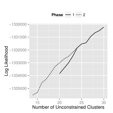
Figure 2: (a) BIC and (b) log-likelihood values for models with different structures. All the clusters are unstructured in the Phase 1 models and the x-axis denotes the total number of clusters. The total number of clusters is 24 for Phase 2 models and the x-axis denotes the number of unconstrained clusters. The remaining clusters have TF-homogeneity.

(a)	(b)

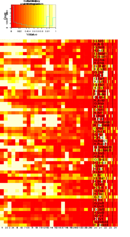
Figure 3: (a) Normalized data for each cell-TF combination at five sub-sampled loci within each cluster. (b) Estimated enrichment probability at each cell-TF combination for each cluster.

We followed the two-phase procedure using BIC from Section 3.4 to select both the number of clusters and the structure of each cluster. In Phase 1, we selected the number of clusters as 24. In Phase 2, we considered two types of structural constraints for each cluster, referred to by TF-homogeneity and cell type-homogeneity and defined as $w_{jk_{1}s}=w_{jk_{2}s}$ if $k_{1}$ and $k_{2}$ corresponded to the same TF or cell type. We found that imposing cell type-homogeneity to any cluster would cause that cluster to be degenerate (i.e., no unit was assigned to that cluster). Therefore, we chose the final model among those with TF-homogeneity structures. The BIC and log likelihood values for different models fitted in both phases are shown in Figure 2. The final model had 24 unconstrained clusters, consisting of $1-\zeta=89.8\%$ of the 10290 loci. The ranges of the estimated distribution parameters among replicates within the same cell type-TF combination is shown in Figure C.12. We notice that these parameters can be substantially different among replicated experiments. This provides further support for our replicate specific parametrization.

To compare the normalized data and the predicted enrichment probability for each cluster, we computed the normalized signals and compared them to the estimated cluster parameters. Figure 3 depicts such normalized signals from five randomly selected loci within each predicted cluster (Figure 3(a)), as well as the predicted enrichment probabilities at the corresponding condition and cluster ($w_{jk2}$’s) (Figure 3(b)). We observe that the estimated enrichment probabilities at the cluster level capture the commonality among loci within each cluster. In addition, each loci cluster exhibits distinct combinatorial patterns of activity across all cell type-TF combination. The cell type-TF combination enriched within each cluster is listed in Table C.9.

Our clustering results are consistent with the existing literature on the TF enrichment networks. For example, cooperating TFs tend to be enriched at the same loci. This pattern can be observed in Figure 3(b) between Bcl3 and Bclaf1. Pol2 and Pol24h8 represent Pol2 experiments with different antibodies. As expected, we observe enrichment at the same loci for these two different version of Pol2 experiments. Moreover, pairs of TFs that have similar binding motifs have similar enrichment probabilities over the clusters. For example, Wang et al. (2012) discovered the UA1 motif as common to both Chd2 and Ets1 and the USF motif for Max, Usf1, and Usf2. Interactions between Taf1 and Tbp have also been studied by Anandapadamanaban et al. (2013). Similar enrichment probabilities of these TFs across clusters can be observed in Figure 3(b). In addition to these observations that are consistent with the literature, our results illustrate how the genome-wide TF association patterns can be attributed to specific clusters. We explored the loci clusters with distinct patterns between cell types (e.g., Pol2 in Cluster 12, Figure 4), TFs from the same families (e.g., Bcl3 v.s. Bclaf1 in Cluster 3, Figure C.13), and TFs with similar genome-wide enrichment (e.g., Max v.s. Usf1 in Cluster 2, Figure C.14) using raw data. We further evaluated each cluster of genes for their KEGG pathway enrichment (Subramanian et al., 2005), and identified 8 KEGG pathways that are significantly enriched in individual clusters (Table 2). Three of our clusters (Clusters 7, 9, and 19) have more than half of their genes in one single pathway. Since KEGG pathways curate the known knowledge of molecular interaction systems, these clusters may be driven by unknown biological processes that warrant further investigation.

(a)	(b)

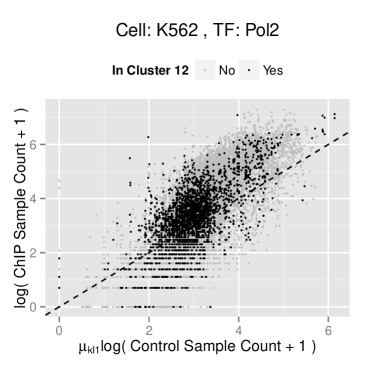
Figure 4: (a, b) Plots of the transformed Pol2 ChIP sample read counts against the transformed control sample read counts for all units in (a) Gm12878 and (b) K562 cells. Data from unenriched units are expected to reside around the 45 degree dashed line.

Table 2: Significantly enriched KEGG pathways across the 24 clusters.

KEGG.name	# Genes	Z Score	Cluster	Cluster
	Overlapped			Size
Protein processing in endoplasmic reticulum	156	5.652	7	391
Fatty acid elongation in mitochondria	7	7.518	8	133
B cell receptor signaling pathway	74	6.016	9	146
Lysine biosynthesis	3	6.53	9	146
D-Glutamine and D-glutamate metabolism	3	5.548	12	184
Vitamin B6 metabolism	4	5.28	14	156
Non-homologous end-joining	12	7.539	17	213
Lysosome	116	5.402	19	187

MBASIC infers the clustering structure based on its own estimates of the state-space profiles. The ENCODE consortium provides the estimated enrichment regions (i.e., peaks) for each experiment in this study. Then, a natural question is whether MBASIC reveals more information compared to clustering of genes based on ENCODE-estimated binary enrichment profiles of TFs. To address this, we created a binary vector for each gene by overlapping its promoter with the ENCODE peaks. Then, we applied the state-of-the-art MClust model (Fraley and Raftery, 2002) to cluster the 10290 promoter regions based on these peak profiles. MClust selected 90 clusters based on BIC. Figure C.15 displays cluster-level estimated enrichment probabilities of TFs across the conditions considered. Compared to Figure 3, we can see that many of the MClust clusters have very similar enrichment profiles. For example, Clusters 51, 7, 8, 32, 54 contained almost no enrichment for any TFs, but are classified as distinct clusters. The association between units across these clusters are thus non-trivial to interpret. In addition, we found that for some conditions, the enrichment states predicted by MBASIC are quite different than those from the ENCODE peak profiles (e.g., Figure 5). This is because the ENCODE peaks are identified by whole genome-wide analysis and may not reflect the differences between the ChIP and control samples at the local promoter regions. MBASIC attains larger raw data fidelity by directly modeling the counts at each unit rather than inheriting results from existing analyses.

(a)	(b)

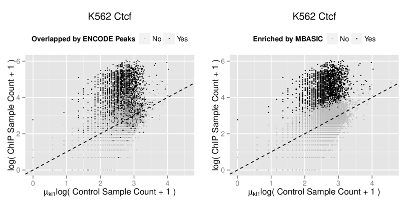
Figure 5: (a, b) Transformed ChIP versus control sample read counts from a Gm12878-Ctcf dataset. Enrichment states are annotated by (a) ENCODE peak profiles and (b) MBASIC estimation. In MBASIC, an observational unit is estimated to be enriched if its enrichment probability satisfies $P(\theta_{ik}=2|Y)>0.5$.

4.2 Genome-wide Identification of +9.5-like Composite Elements

Johnson et al. (2012) and Gao et al. (2013) described the requirement of the intronic +9.5 site, an Ebox-GATA composite element located at chr6: 88143884-88157023 in the mouse genome (genome version mm9), to establish the hematopoietic stem/progenitor cell (HSC) compartment in the fetal liver and for hematopoietic stem cell genesis in the aorta-gonad-mesonephros (AGM), respectively. Furthermore, Johnson et al. (2012) and Hsu et al. (2013) showed that heterozygous +9.5 mutations cause a human immunodeficiency associated with myelodysplastic syndrome (MDS) and acute myeloid leukemia (AML). Because the +9.5 site is the only known cis-element deletion of which depletes fetal liver HSCs and is lethal at E13-14 of embryogenesis, identifying additional loci that have similar functionality is extremely important for establishing mechanisms that enable GATA factor-bound regions with nonredundant activity and have the potential to reveal novel targets for therapeutic modulation of hematopoiesis. In this application, we identified 4803 genomic regions with the Ebox-GATA motif (CATCTG-N[7-9]-AGATAA where N[7-9] denotes a variable size spacer of 7 and 9 nucleotides) in the human genome (genome version hg19). We considered a 150 bps window anchored at each of the 4803 composite elements as the observational unit. To analyze the TF occupancy activities at these units and identify a group of composite elements with occupancy profiles similar to that of the +9.5 composite element, we downloaded all ChIP-seq data for the Huvec and K562 cells from Gerstein et al. (2012). In total, the data set contained 224 replicates spanning $K=84$ experimental conditions and 77 TFs.

We used negative binomial distributions with $S=2$ states, where $s=1$ denoted the unenriched (unoccupied) state, in the MBASIC framework. We chose $\gamma_{ikl1}=1+x_{ik}$, where $x_{ik}$ is the count for unit $i$ from the matching control experiment for condition $k$, to incorporate data from the accompanying control experiments of the ChIP samples. For $s=2$, we utilized the following mixture distribution to account for the heavy tails observed in the raw data:

$$Y_{ikl}-3|\theta_{ik}=2{\buildrel\rm ind.\over{\sim}}\nu_{ikl}NB(\mu_{kl2},\sigma_{kl2})+(1-\nu_{ikl})NB(\mu_{kl3},\sigma_{kl3}),$$

$$\nu_{ik}{\buildrel\rm i.i.d.\over{\sim}}Bernoulli(v_{kl}).$$

Here, the constant 3 represents the minimum count threshold for enrichment estimation. The use of mixture distributions to capture heavy tailed count data was previously considered by Zuo and Keleş (2013). We note that an alternative approach to capture heavy tailed counts would be to fit a model using $S=3$ states, with $s=2,3$ representing two distinct enrichment components. Such an approach would differ from the proposed approach in a subtle yet important way. In this alternative approach, allocation of each unit to different enrichment components would affect the clustering estimation, while in our approach, clustering is only determined by the enrichment status of the individual unit regardless of which enrichment component it follows. The E-M algorithm for this setting requires a slight modification as discussed in Section A.2.

Figure 6: Posterior enrichment probability (i.e,. $P(\theta_{ik}=2|Y)$) for all units in the three clusters. The right most column of the C3 cluster corresponds to the +9.5 element.

Following the two phase model selection procedure using BIC, we selected the model with 3 clusters, 2 of which were cell type-homogeneous. The ranges of the estimated distribution parameters among replicates within the same condition are displayed in Figures C.16 and C.17. The three clusters (denoted by C1, C2, and C3) included 332, 837, 157 composite elements, respectively, and the remaining 3477 composite elements were identified as singletons. A heatmap for the enrichment probability of each unit under each cell type-TF combination across the three clusters is shown in Figure 6. The +9.5 element is a member of cluster C3 which consists of a total of 157 +9.5-like composite elements. A detailed genomic annotation of these elements are provided in Table LABEL:tbl:pa_result. Notably, 46% of the C3 elements reside in intronic regions and 42% of these are within first intron. Only 15% of the cluster are located up to 10Kb upstream of transcription start sites.

A detailed analysis of Figure 6 reveals that cluster C3 is driven by several transcription factors with known associations to GATA2. First, we note that a large fraction of the C3 loci are bound by BRG1. The chromatin remodeler BRG1 is involved in GATA1-mediated chromatin looping (Kim et al., 2009a, b) and co-localizes with GATA1 at some chromatin sites (Hu et al., 2011). BRG1 has broad functions in many cell types; however, conditional knockouts of BRG1 reveal its importance in specific cell and tissue contexts (Holley et al., 2014). Another factor that clearly stands out as having a GATA2-like profile in cluster C3 is ETS1. Our prior work identified the propensity of occupied GATA motifs to reside near Ets motifs (Linneman et al., 2011) and Doré et al. (2012) has highlighted GATA2-ETS co-localization.

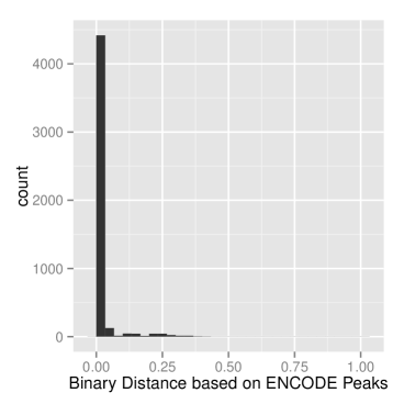
Figure 7: Proportion of overlap between the top ranked +9.5-like composite elements identified by MBASIC and ENCODE peak profiles. The overlap proportion is calculated by considering the same number of top ranked units (x-axis) in both the ENCODE-based and MBASIC-based similarities to the +9.5 site. The dashed lines mark that 78.3% of the C3 units are ranked in the top 157 based on the ENCODE peak profiles.

We next performed an alternative naive analysis by utilizing the list of peaks provided by the ENCODE project. As in the case of the Transcription Factor Enrichment Network example of Section 4.1, these peaks, provided by the ENCODE consortium, were identified by analyzing each dataset individually with ENCODE’s uniform ChIP-seq processing pipeline. Figure C.18 displays the ENCODE peak profiles for our cell type-TF conditions. For each of the 4803 composite elements, we constructed a peak profile, which is a binary vector indicating whether the element overlaps with the ENCODE peaks for each cell type-TF combination. We then computed the peak profile based similarity between the +9.5 site and each the of the composite elements using the R function dist.binary with the ”Jaccard index” option. For comparison, we computed pseudo-binary similarities between each element and the +9.5 site using the MBASIC estimated enrichment probabilities across all conditions. We then ranked the composite elements based on both ENCODE and MBASIC estimated similarities. Figure 7 provides a comparison of the two lists as a function of top ranking composite elements. Overall, we observe that the rankings based on MBASIC estimation are consistent with the rankings based on the ENCODE peak profiles.

(a)
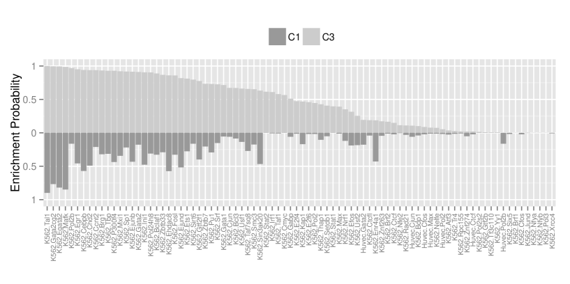
(b)	(c)

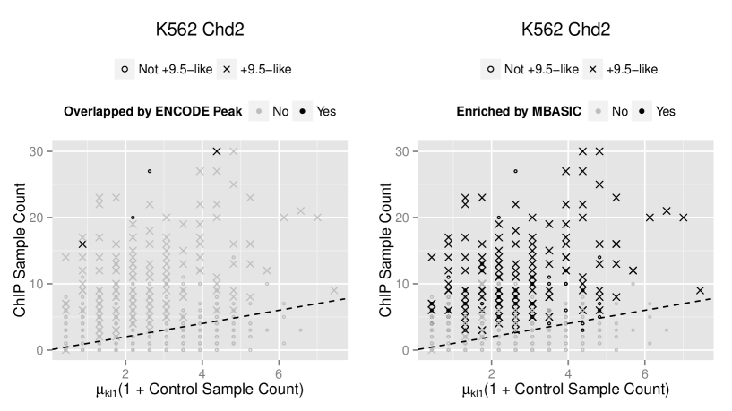
Figure 8: (a) Top half: Enrichment probabilities for the C3 units across all experimental conditions estimated by MBASIC. Bottom half: Proportion of C3 units that are overlapped by the ENCODE peaks for each condition. (b, c) ChIP sample read counts against normalized control sample read counts for one replicate of K562-Chd2 dataset. Enrichment status are annotated by (a) the ENCODE peak profiles and (c) MBASIC prediction.

Although the rankings of the composite elements with respect to their +9.5 similarity using both the ENCODE peak profiles and MBASIC estimation were quite similar, the two approaches resulted in different enrichment estimation at the individual TF-cell combination level. Figure 8(a) compares the estimated cluster-level enrichment probabilities of each cell type-TF combination for cluster C3 against their average ENCODE peak profiles and highlights the difference between the two procedures. To further investigate these differences, we plotted the raw data for individual replicates and compared the composite elements that were estimated to be enriched by the two methods. An example using data from K562-Chd2 is displayed in Figures 8(b) and (c). Although many elements have significantly higher counts in the ChIP sample compared to the control sample, they are not identified as occupied by Chd2 in K562 according to ENCODE peak annotation. Another example using a replicate from K562-Yy1 is shown in Figure C.19, where several elements with zero ChIP count are overlapped by ENCODE peaks. These results indicate that MBASIC provides a grouping of the Ebox-GATA composite elements that is more consistent with the raw data compared to grouping based on ENCODE peak annotation.

5 Conclusions and Discussion

Clustering analysis based on an underlying state-space is a common problem for many genomic and epigenomic studies where multiple data sets over many observational units are integrated. In this paper, we developed a unified statistical framework, called MBASIC, for addressing these class of problems. MBASIC simultaneously projects the observations onto a hidden state-space and infers clustered units in this space. The hierarchical structure of MBASIC enables the information of the state-space clusters to be fed back into the projection of the raw data, thus reinforces the accuracy of predicting the state-space states of individual units. The MBASIC framework offers flexibility in a number of aspects of experimental design, such as different numbers of replicates under individual experimental conditions and missing values. Additionally, it is applicable to many parametric distributions. Our computational studies highlighted good operating characteristics of MBASIC and the two genomic applications illustrated how large numbers of ChIP-seq datasets can be integrated for addressing specific problems. In both of the applications, MBASIC algorithm converged within 20 minutes for a fixed model on a 64 bit machine with Intel Xeon 3.0GHz processor and 64GB of RAM. For model selection, we utilized R package snow to implement the 2-phase procedure with parallel fitting of different candidate models using a 8-core 64 bit, 64GB RAM machine with 8 Intel Xeon 3.0GHz processors. These runs were completed under 2 hours. The computational efficiency of our model depends on the simple, closed-form updates in our E-M algorithm. Such a mathematical form is due, at least in part, to our modeling assumption that the rows of our state-space matrix is clustered. We have argued that this assumption, as compared to the PCA-type model structures, offers easier interpretation and is well suited for many genomic applications. MBASIC is available as R package mbasic at https://github.com/chandlerzuo/mbasic.

Appendix A Details of the Expectation-Maximization (EM) Algorithms

A.1 Derivation for the E-step

We derive the expressions for the E-step updates of our algorithm in Eqns. (12), (13), (14), (15) as well as the marginal likelihood in Eqns. (9) and (10).

In what follows, we let $\theta_{iks}$ denote $1\{\theta_{ik}=s\}$. The joint density of $(z,b,\theta,Y)$ is given by:

$$f(z,b,\theta,y)=\prod_{i=1}^{I}\zeta^{b_{i}}(1-\zeta)^{1-b_{i}}\cdot\prod_{i=1}^{I}\prod_{j=1}^{J}\pi_{j}^{z_{ij}}\cdot\prod_{i=1}^{I}\prod_{k=1}^{K}\prod_{s=1}^{S}\left[f_{iks}(\prod_{j=1}^{J}w_{jks}^{z_{ij}})^{1-b_{i}}p_{is}^{b_{i}}\right]^{\theta_{iks}},$$ (24)

where $f_{iks}=\prod_{l=1}^{n_{k}}f(y_{ikl}|\mu_{kls},\sigma_{kls},\gamma_{ikls})$. The following elementary equality is used repeatedly throughout the rest of the derivations in this section.

$$\sum_{\sum_{j}a_{ij}=1,a_{ij}\in\{0,1\}}\prod_{i}\prod_{j}b_{ij}^{a_{ij}}=\prod_{i}\left(\sum_{j}b_{ij}\right).$$

The joint density of $(z,b,Y)$ can be calculated from Eqn. (24):

$$f(z,b,y)= \sum_{\sum_{s}\theta_{iks}=1}f(z,b,\theta,y)$$ (25)

$$= \prod_{i=1}^{I}\zeta^{b_{i}}(1-\zeta)^{1-b_{i}}\cdot\prod_{i=1}^{I}\prod_{j=1}^{J}\pi_{j}^{z_{ij}}\cdot\sum_{\sum_{s}\theta_{iks}=1}\prod_{i=1}^{I}\prod_{k=1}^{K}\prod_{s=1}^{S}\left[f_{iks}\left(\prod_{j=1}^{J}w_{jks}^{z_{ij}}\right)^{1-b_{i}}p_{is}^{b_{i}}\right]^{\theta_{iks}}$$

$$= \prod_{i=1}^{I}\zeta^{b_{i}}(1-\zeta)^{1-b_{i}}\cdot\prod_{i=1}^{I}\prod_{j=1}^{J}\pi_{j}^{z_{ij}}\cdot\prod_{i=1}^{I}\prod_{k=1}^{K}\left[\sum_{s=1}^{S}f_{iks}\left(\prod_{j=1}^{J}w_{jks}^{z_{ij}}\right)^{1-b_{i}}p_{is}^{b_{i}}\right].$$

Since

$$\sum_{s=1}^{S}f_{iks}\left(\prod_{j=1}^{J}w_{jks}^{z_{ij}}\right)^{1-b_{i}}p_{is}^{b_{i}}=\prod_{j=1}^{J}\left[\sum_{s=1}^{S}f_{iks}w_{jks}^{1-b_{i}}p_{is}^{b_{i}}\right]^{z_{ij}},$$

Eqn. (25) can be rewritten as:

$$f(z,b,y)=\prod_{i=1}^{I}\zeta^{b_{i}}(1-\zeta)^{1-b_{i}}\cdot\prod_{i=1}^{I}\prod_{j=1}^{J}\left[\pi_{j}\prod_{k=1}^{K}\left(\sum_{s=1}^{S}f_{iks}w_{jks}^{1-b_{i}}p_{is}^{b_{i}}\right)\right]^{z_{ij}}.$$ (26)

The joint distribution of $(b,Y)$ can be calculated from Eqn. (26):

$$f(b,y)= \sum_{\sum_{j}z_{ij}=1}f(z,b,y)$$ (27)

$$= \prod_{i=1}^{I}\zeta^{b_{i}}(1-\zeta)^{1-b_{i}}\cdot\sum_{\sum_{j}z_{ij}=1}\prod_{i=1}^{I}\prod_{j=1}^{J}\left[\pi_{j}\prod_{k=1}^{K}\left(\sum_{s=1}^{S}f_{iks}w_{jks}^{1-b_{i}}p_{is}^{b_{i}}\right)\right]^{z_{ij}}$$

$$= \prod_{i=1}^{I}\zeta^{b_{i}}(1-\zeta)^{1-b_{i}}\cdot\prod_{i=1}^{I}\left[\sum_{j=1}^{J}\pi_{j}\prod_{k=1}^{K}\left(\sum_{s=1}^{S}f_{iks}w_{jks}^{1-b_{i}}p_{is}^{b_{i}}\right)\right].$$

We note that

$$\sum_{j=1}^{J}\pi_{j}\prod_{k=1}^{K}\left(\sum_{s=1}^{S}f_{iks}w_{jks}^{1-b_{i}}p_{is}^{b_{i}}\right)=\left[\sum_{j=1}^{J}\pi_{j}\prod_{k=1}^{K}\left(\sum_{s=1}^{S}f_{iks}w_{jks}\right)\right]^{1-b_{i}}\left[\prod_{k=1}^{K}\left(\sum_{s=1}^{S}f_{iks}p_{is}\right)\right]^{b_{i}}.$$

Then, Eqn. (27) can be rewritten as:

$$f(b,y)=\prod_{i=1}^{I}\left[(1-\zeta)\sum_{j=1}^{J}\pi_{j}\prod_{k=1}^{K}\left(\sum_{s=1}^{S}f_{iks}w_{jks}\right)\right]^{1-b_{i}}\left[\zeta\prod_{k=1}^{K}\left(\sum_{s=1}^{S}f_{iks}p_{is}\right)\right]^{b_{i}}.$$ (28)

We can calculate the marginal density of $Y$, given in Eqn. (9), from Eqn. (28) as:

$$f(y)=\sum_{b_{i}\in\{0,1\}}f(b,y)=\prod_{i=1}^{I}\left[(1-\zeta)\sum_{j=1}^{J}\pi_{j}\prod_{k=1}^{K}\left(\sum_{s=1}^{S}f_{iks}w_{jks}\right)+\zeta\prod_{k=1}^{K}\left(\sum_{s=1}^{S}f_{iks}p_{is}\right)\right].$$ (29)

Eqn. (10) can be obtained similarly. Moreover, we can rewrite (25) as

$$f(z,b,y)=\prod_{i=1}^{I}\left[\zeta\prod_{k=1}^{K}\sum_{s=1}^{S}f_{iks}p_{is}\right]^{b_{i}}\left[(1-\zeta)\prod_{j=1}^{J}\prod_{k=1}^{K}\left(\sum_{s=1}^{S}f_{iks}w_{jks}\right)^{z_{ij}}\right]^{1-b_{i}}\cdot\prod_{i=1}^{I}\prod_{j=1}^{J}\pi_{j}^{z_{ij}}$$ (30)

by using

$$\sum_{s=1}^{S}f_{iks}\left(\prod_{j=1}^{J}w_{jks}^{z_{ij}}\right)^{1-b_{i}}p_{is}^{b_{i}}=\left[\prod_{j=1}^{J}\left(\sum_{s=1}^{S}f_{iks}w_{jks}\right)^{z_{ij}}\right]^{1-b_{i}}\left[\sum_{s=1}^{S}f_{iks}p_{is}\right]^{b_{i}}.$$

Thus, the density of $(z,Y)$ can be calculated as:

$$f(z,y)= \sum_{b_{i}\in\{0,1\}}\prod_{i=1}^{I}\left[\zeta\prod_{k=1}^{K}\left(\sum_{s=1}^{S}f_{iks}p_{is}\right)\right]^{b_{i}}\left[(1-\zeta)\prod_{j=1}^{J}\prod_{k=1}^{K}\left(\sum_{s=1}^{S}f_{iks}w_{jks}\right)^{z_{ij}}\right]^{1-b_{i}}\cdot\prod_{i=1}^{I}\prod_{j=1}^{J}\pi_{j}^{z_{ij}}$$ (31)

$$= \prod_{i=1}^{I}\left[\zeta\prod_{k=1}^{K}\left(\sum_{s=1}^{S}f_{iks}p_{is}\right)+(1-\zeta)\prod_{j=1}^{J}\prod_{k=1}^{K}\left(\sum_{s=1}^{S}f_{iks}w_{jks}\right)^{z_{ij}}\right]\cdot\prod_{i=1}^{I}\prod_{j=1}^{J}\pi_{j}^{z_{ij}}$$

$$= \prod_{i=1}^{I}\prod_{j=1}^{J}\left[\pi_{j}\zeta\prod_{k=1}^{K}\left(\sum_{s=1}^{S}f_{iks}p_{is}\right)+\pi_{j}(1-\zeta)\prod_{k=1}^{K}\left(\sum_{s=1}^{S}f_{iks}w_{jks}\right)\right]^{z_{ij}}.$$

Using Eqns. (28) and (29), we obtain Eqn. (12) as

$$E[b_{i}|Y]=\frac{\zeta\prod_{k=1}^{K}\left(\sum_{s=1}^{S}f_{iks}p_{is}\right)}{(1-\zeta)\sum_{j=1}^{J}\pi_{j}\prod_{k=1}^{K}\left(\sum_{s=1}^{S}f_{iks}w_{jks}\right)+\zeta\prod_{k=1}^{K}\left(\sum_{s=1}^{S}f_{iks}p_{is}\right)}.$$ (32)

Similarly, using Eqns. (31) and (29), we have

$$E[z_{ij}|Y]=\frac{\pi_{j}\zeta\prod_{k=1}^{K}\left(\sum_{s=1}^{S}f_{iks}p_{is}\right)+(1-\zeta)\pi_{j}\prod_{k=1}^{K}\left(\sum_{s=1}^{S}f_{iks}w_{jks}\right)}{\zeta\prod_{k=1}^{K}\sum_{s=1}^{S}f_{iks}p_{is}+(1-\zeta)\sum_{j=1}^{J}\pi_{j}\prod_{k=1}^{K}\left(\sum_{s=1}^{S}f_{iks}w_{jks}\right)}.$$ (33)

Using Eqns. (26) and (27), we have

$$E[z_{ij}|b,Y]=\frac{\pi_{j}\prod_{k=1}^{K}\left(\sum_{s=1}^{S}f_{iks}w_{jks}^{1-b_{i}}p_{is}^{b_{i}}\right)}{\sum_{j=1}^{J}\pi_{j}\prod_{k=1}^{K}\left(\sum_{s=1}^{S}f_{iks}w_{jks}^{1-b_{i}}p_{is}^{b_{i}}\right)}.$$ (34)

Eqns. (34) and (32) together results in Eqn. (13). Using Eqns. (24) and (25), we have

$$E[\theta_{iks}|z,b,Y]=\frac{f_{iks}\left(\prod_{j=1}^{J}w_{jks}^{z_{ij}}\right)^{1-b_{i}}p_{is}^{b_{i}}}{\sum_{s=1}^{S}f_{iks}\left(\prod_{j=1}^{J}w_{jks}^{z_{ij}}\right)^{1-b_{i}}p_{is}^{b_{i}}}.$$ (35)

Therefore, we obtain Eqn. (14) by using Eqns. (27), (34), and (35):

$$E[\theta_{iks}z_{ij}(1-b_{i})|Y]= [1-E(b_{i}|Y)]E(z_{ij}|b_{i}=0,Y)E(\theta_{iks}|b_{i}=0,z_{ij}=1,Y)$$ (36)

$$= \frac{(1-\zeta)\sum_{j=1}^{J}\pi_{j}\prod_{k=1}^{K}\left(\sum_{s=1}^{S}f_{iks}w_{jks}\right)}{(1-\zeta)\sum_{j=1}^{J}\pi_{j}\prod_{k=1}^{K}\left(\sum_{s=1}^{S}f_{iks}w_{jks}\right)+\zeta\prod_{k=1}^{K}\left(\sum_{s=1}^{S}f_{iks}p_{is}\right)}\cdot$$

$$\frac{\pi_{j}\prod_{k=1}^{K}\left(\sum_{s=1}^{S}f_{iks}w_{jks}\right)}{\sum_{j=1}^{J}\pi_{j}\prod_{k=1}^{K}\left(\sum_{s=1}^{S}f_{iks}w_{jks}\right)}\cdot\frac{f_{iks}w_{jks}}{\sum_{s=1}^{S}f_{iks}w_{jks}}.$$

Finally, we obtain Eqn. (15) using Eqns. (35) and (27):

$$E(\theta_{iks}b_{i}|Y)= E(b_{i}|Y)E(\theta_{iks}|b_{i}=1,Y)$$ (37)

$$= \frac{\zeta\prod_{k=1}^{K}\left(\sum_{s=1}^{S}f_{iks}p_{is}\right)}{(1-\zeta)\sum_{j=1}^{J}\pi_{j}\prod_{k=1}^{K}\left(\sum_{s=1}^{S}f_{iks}w_{jks}\right)+\zeta\prod_{k=1}^{K}\left(\sum_{s=1}^{S}f_{iks}p_{is}\right)}\cdot\frac{f_{iks}p_{is}}{\sum_{s=1}^{S}f_{iks}p_{is}}.$$

A.2 EM Algorithm with Mixture Data Distributions

An important extension of the MBASIC model is to allow multiple mixture components within each state. For example, our model in Section 4.2 models the data from state $s=2$ as a mixture of two negative binomial distributions following the well motivated model of Kuan et al. (2011):

$$Y_{ikl}-3|\theta_{ik}=2\sim\nu_{ikl}NB(\mu_{kl2},\sigma_{kl2})+(1-\nu_{ikl})NB(\mu_{kl3},\sigma_{kl3}),$$

$$\nu_{ikl}\sim Bernoulli(v_{kl}),$$

where the constant $3$ denotes the minimum number of reads required to be in state $\theta=2$. In this section, we describe the general algorithm for such extensions. We assume that data from state $s$ has a distribution of $m_{s}$ components:

$$Y_{ikl}|\theta_{iks}=1\sim\sum_{r=1}^{m_{s}}v_{klsr}f_{sr}(\cdot|\mu_{klsr},\sigma_{klsr},\gamma_{iklsr}).$$

This can be written in a hierarchical form, using $\nu_{iklsr}$ as the hidden variable indicating the mixture component within the state:

$$(\nu_{iklsr})_{1\leq r\leq m_{s}}\sim Multinom(1,(v_{klsr})_{1\leq r\leq m_{s}}),~{}Y_{ikl}|\theta_{iks}=1,\nu_{iklsr}=1~{}\sim~{}f_{sr}(\cdot|\mu_{klsr},\sigma_{klsr},\gamma_{iklsr}).$$ (38)

Here, we allow the distribution parameters $\mu$ and $\sigma$ as well as the prior information derived $\gamma$ to depend on the component. Let $f_{iklsr}=f_{sr}(y_{ikl}|\mu_{klsr},\sigma_{klsr},\gamma_{iklsr})$. The joint density for this model is:

$$f(z,b,\theta,\nu,y)= \prod_{i=1}^{I}\zeta^{b_{i}}(1-\zeta)^{1-b_{i}}\cdot\prod_{i=1}^{I}\prod_{j=1}^{J}\pi_{j}^{z_{ij}}\cdot\prod_{i=1}^{I}\prod_{k=1}^{K}\prod_{l=1}^{n_{k}}\prod_{s=1}^{S}\prod_{r=1}^{m_{s}}v_{iklsr}^{\nu_{klsr}}$$ (39)

$$\cdot \prod_{i=1}^{I}\prod_{k=1}^{K}\prod_{s=1}^{S}\left[\left(\prod_{l=1}^{n_{k}}\prod_{r=1}^{m_{s}}f_{iklsr}^{\nu_{iklsr}}\right)\left(\prod_{j=1}^{J}w_{jks}^{z_{ij}}\right)^{1-b_{i}}p_{is}^{b_{i}}\right]^{\theta_{iks}}.$$

Let $f_{iks}=\prod_{l=1}^{n_{k}}(\sum_{r=1}^{m_{s}}v_{klsr}f_{iklsr})$, then the joint density for $z,b,\theta,Y$ can be expressed exactly the same as Eqn. (24). Therefore, the M-step updates for $W$, $P$, $\zeta$ and $\pi$ are not changed, with the related E-step quantities computed as Eqns. (12), (13), (14), (15). We only need to modify the algorithm to estimate variables that depend on the component index $r$: $\mu$, $\sigma$, and $v$.

The related quantities that need to be computed are $E[\nu_{iklsr}|Y]$ and $E[\theta_{iks}\nu_{iklsr}|Y]$. By Eqn. (39), we have

$$P(\nu_{iklsr}=1|\theta_{iks}=0)=v_{klsr},~{}~{}P(\nu_{iklsr}=1|\theta_{iks}=1)=\frac{v_{klsr}f_{iklsr}}{\sum_{r=1}^{m_{s}}v_{klsr}f_{iklsr}}.$$

Therefore, we have

$$E[\theta_{iks}\nu_{iklsr}|Y]=E[\theta_{iks}|Y]\frac{v_{klsr}f_{iklsr}}{\sum_{r=1}^{m_{s}}v_{klsr}f_{iklsr}},$$ (40)

where $E[\theta_{iks}|Y]=\sum_{j=1}^{J}E[\theta_{iks}(1-b_{i})z_{ij}|Y]+E[\theta_{iks}b_{i}|Y]$ and can be computed by Eqns. (36) and (37). As a result,

$$E[\nu_{iklsr}|Y]=(1-E[\theta_{iks}|Y])v_{klsr}+E[\theta_{iks}\nu_{iklsr}|Y].$$ (41)

Given Eqns. (40) and (41), the M-step update for $v_{klsr}$ is:

$$v_{klsr}^{(t)}=\frac{\sum_{i=1}^{I}E[\nu_{iklsr}|\hat{\phi}^{(t-1)}]}{I}.$$

The M-step updates for $\mu_{klsr}$, $\sigma_{klsr}$ can be derived using Eqn. (40). For the negative binomial distribution, as in Section 4.2, we have

$$\hat{\mu}_{klsr}^{(t)}\sum_{i=1}^{I}\gamma_{ikls}E\left[\theta_{iks}v_{iklsr}|\hat{\phi}^{(t-1)}\right] =\sum_{i=1}^{I}E\left[\theta_{iks}\nu_{iklsr}|\hat{\phi}^{(t-1)}\right](Y_{ikl}-3),$$

$$\sum_{i=1}^{I}E\left[\theta_{iks}v_{iklsr}|\hat{\phi}^{(t-1)}\right]\left[\hat{\mu}_{klsr}^{(t)2}\gamma_{ikls}^{2}\left(1+\frac{1}{\hat{\sigma}_{klsr}^{(t)}}\right)+\hat{\mu}_{klsr}^{(t)}\gamma_{ikls}\right] =\sum_{i=1}^{I}E\left[\theta_{iks}v_{iklsr}|\hat{\phi}^{(t-1)}\right](Y_{ikl}-3)^{2}.$$

Appendix B Simulation Studies

This section presents six broad simulation studies to evaluate the performance of MBASIC. Each simulation study had multiple settings as outlined in Table 1 of the main article. We introduced the following four families of distributions in our main article:

• Log-normal Distribution. $LN(\mu_{kls}\gamma_{ikls},\sigma_{kls})$ with a density function:

  $$f_{s}(y|\mu_{kls},\sigma_{kls},\gamma_{ikls})=\frac{1}{\sqrt{2\pi}\sigma_{kls}}\exp\left\{-\frac{(\log(y+1)-\mu_{kls}\gamma_{ikls})^{2}}{2\sigma_{kls}^{2}}\right\}.$$ (42)

• Negative Binomial Distribution. $NB(\mu_{kls}\gamma_{ikls},\sigma_{kls})$ with a density function:

  $$f_{s}(y|\mu_{kls},\sigma_{kls},\gamma_{ikls})=\frac{\Gamma(y+\sigma_{kls})}{\Gamma(\sigma_{kls})\Gamma(y+1)}\frac{(\mu_{kls}\gamma_{ikls})^{y}\sigma_{kls}^{\sigma_{kls}}}{(\mu_{kls}\gamma_{ikls}+\sigma_{kls})^{y+\sigma_{kls}}}.$$ (43)

• Binomial Distribution. $Binom(\gamma_{ikls},\mu_{kls})$ with a density function:

  $$f_{s}(y|\mu_{kls},\gamma_{ikls})={\gamma_{ikls}\choose y}\mu_{kls}^{y}(1-\mu_{kls})^{\gamma_{ikls}-y}.$$ (44)

• Degenerate Distribution:

  $$f_{s}(y|\mu_{kls},\sigma_{kls},\gamma_{ikls})=I(y=s).$$ (45)

B.1 Simulation Study 1

The first simulation study investigated the performance of MBASIC when the true value of $J$ was known and there were no structured clusters. We set the number of observational units as $I=4000$ and the number of clusters as $J=20$. The number of conditions was set to $K=30$, and within each condition the numbers of replicates varied as $n_{k}=1,2,3$, each with probability 0.3, 0.5, and 0.2. The size of the hidden state space was varied at three levels: $S=2,3,4$. We simulated data under three distributional families: log-normal (LN) (3), negative binomial (NB) (4), and binomial (Bin) (5). We also varied the proportion of singleton units $\zeta$ at 0, 0.1 and 0.4. For simplicity, we set $\gamma_{ikls}=1$ in all distributions.

B.1.1 Parameter Settings

Parameters $w_{jks}$’s and $p_{is}$’s generate the hidden state variables $\theta_{ik}$’s. We set them as follows. For different values of $k$, $j$, and $i$, the vectors $w_{jk\cdot}=(w_{jks}:1\leq s\leq S)$ and $p_{i\cdot}=(p_{is}:1\leq s\leq S)$ were simulated independently, each following an S-dimensional Dirichlet distribution $Dir(\alpha,\cdots,\alpha)$. We chose a uniform concentration parameter of $\alpha=0.2$ for all dimensions to ensure that for each vector $w_{jk\cdot}$ or $p_{i\cdot}$, the probability mass tended to concentrate on one component. This controlled the conditional variance of $(\theta_{ik}|b_{i},z_{ij})$. An increased value of $\alpha$ would increase the conditional variance of $\theta_{ik}$, thus make it more difficult to recover $w_{jks}$’s and $p_{is}$’s.

The settings for parameters $\mu_{kls}$’s and $\sigma_{kls}$’s were important. These parameters connected hidden states $\theta_{ik}$’s to the observed values $Y_{ikl}$’s. In general, recovering hidden states from the observed data is more difficult if: (1) differences of the mean values $\mu_{kls}$’s between the states are small; (2) variances of the distributions within each state are large. To control these two aspects at reasonable levels, we set these parameters as follows:

• For log-normal distributions (3), we set $\xi_{s}=2+\log(4s-3)$, simulated $\mu_{kls}\sim N(\xi_{s},0.05^{2})$, and set $\sigma_{kls}=0.5$;

• For negative binomial distributions (4), we set $\xi_{s}=8s-6$, simulated $\mu_{kls}\sim N(\xi_{s},0.5^{2})$, and set $\sigma_{kl1}=2.82$, $\sigma_{kls}=5$ for $s=2,~{}3,~{}4$;

• For binomial distributions (5), we simulated $\mu_{kls}\sim Beta(3s,3(S+1-s))$, and $\gamma_{ikl1}=\gamma_{ikl2}=\cdots=\gamma_{iklS}\sim Pois(10)$.

a) Real Data	b) Log-Normal
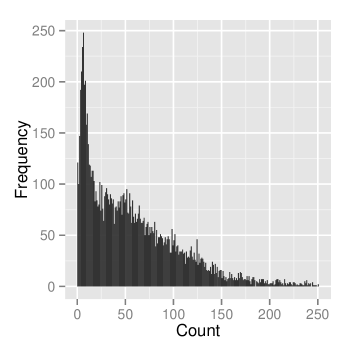
c) Negative Binomial	d) Binomial

Figure B.1: Histograms for a) a real data set from a K562 Pol2 replicate in Section 4.1 of our main article; and simulated data from one condition based on one simulation for the b) Log-Normal, c) Negative Binomial and d) Binomial distribution with S=4 states.

Figure B.1 displays the histograms of $Y_{1,i,l},\quad 1\leq i\leq I$ from one of the simulated data sets for all the three distributions with $S=4$ components. For comparison, we also present the histogram of an actual data set from the analysis in Section 4 of our main article. We observe that the mixture distribution of our simulated data with log-normal or negative-binomial distributions closely follow the real data.

B.1.2 Alternative Approaches for Benchmarking MBASIC

The MBASIC algorithm is summarized as Algorithm 2:

Algorithm 2 MBASIC

  for $t=1,~{}2,\cdots$ until convergence do

     Expectation-Step: Compute the conditional expectations $E[I(\theta_{ik}=s)|\hat{\phi}^{(t-1)}]$, $E[b_{i}|\hat{\phi}^{(t-1)}]$, $E[I(\theta_{ik}=s)b_{i}|\hat{\phi}^{(t-1)}]$, $E[z_{ij}(1-b_{i})|\hat{\phi}^{(t-1)}]$, $E[I(\theta_{ik}=s)z_{ij}(1-b_{i})|\hat{\phi}^{(t-1)}]$;

     Maximization-Step: Update estimates for parameters $\mu_{kls}$, $\sigma_{kls}$, $\zeta$, $\pi_{j}$, $w_{jks}$, $p_{is}$.

  end for

To the best of our knowledge, there are currently no existing methods suited for the general setup of MBASIC. There are, however, algorithms tailored for analyzing specific data types with hierarchical state-space models similar to MBASIC. These algorithms largely fall into two categories. In the first category, estimation for the state-space variables are separated from state-space clustering. Some examples include Cheng et al. (2011), Gerstein et al. (2012), Ji et al. (2013), Neph1 et al. (2012). In the second category, distributional parameters for each experimental replicate are estimated first. These parameters are then fixed, and the state-space variables and the clustering structure are estimated jointly conditional on these estimates. Examples of this approach include Wei et al. (2012), Zeng et al. (2013), and Wei et al. (2015).

Table B.1: Simulation Study 1. A summary of the benchmark algorithms that are compared to MBASIC. Neither SE-MC nor PE-MC perform joint estimation of the model parameters. SE-* algorithms estimate the data-specific model parameters and state-space as a first step and then cluster the state variables. PE-* algorithms estimate data-specific model parameters and fixes these in joint estimation of the state-space and clustering. ^∗ Denotes distributional parameters for each experimental replicate.

Algorithm	Is State-space	Is Parameter∗	Clustering	Include
	Estimation Joint	Estimation Joint	model	singletons
	with Clustering?	with Clustering?
MBASIC	Joint	Joint	Mixture model	Yes
SE-HC	Separate	Separate	Hierarchical clustering	No
SE-MC	Separate	Separate	Mixture model	Yes
PE-MC	Joint	Separate	Mixture model	Yes
MBASIC0	Joint	Joint	Mixture model	No
SE-MC0	Separate	Separate	Mixture model	No
PE-MC0	Joint	Separate	Mixture model	No

To compare the general implementation of MBASIC as in Algorithm 2 with these existing model fitting ideas, we designed six benchmark algorithms. Table B.1 provides a summary of these algorithms. Two of these algorithms, SE-HC (State-space Estimation followed by Hierarchical Clustering) and SE-MC (State-space Estimation followed by Mixture model Clustering), treat the state-space mapping step and the state-space clustering separately. The third algorithm, PE-MC (Parameter Estimation followed by Mixture model Clustering), separates experiment-specific distributional parameter estimation from the joint estimation of other parameters.

For all the three algorithms, in the first step, observations from each experimental condition $\{Y_{ikl}:1\leq i\leq I,1\leq l\leq n_{k}\}$ are fitted according to the following model:

$$(Y_{ikl}|\theta_{ik}=s)\sim f_{s}(\cdot|\mu_{kls},\sigma_{kls},\gamma_{ikls}),\quad P(\theta_{ik}=s)=q_{ks}.$$ (46)

The standard E-M algorithm can be used for the first step and results in estimates of $q_{ks}$, $\mu_{kls}$, $\sigma_{kls}$ as well as the posterior estimates for the state space $P(\theta_{ik}=s|Y)$. In the second step, SE-MC and SE-HC cluster the observational units based on the estimated $P(\theta_{ik}=s|Y)$ from the first step. SE-HC (Algorithm 3) uses hierarchical clustering, while SE-MC (Algorithm 4) uses MBASIC with degenerate distributions (6) for clustering. The second step of PE-MC (Algorithm 5) is similar to Algorithm 2, except that parameters $\mu_{kls}$, $\sigma_{kls}$’s are not updated.

In addition to joint fitting of all model parameters, another important feature of MBASIC is its inclusion of the singleton cluster $\mathscr{C}_{0}$. To the best of our knowledge, this feature is not included in similar models such as Wei et al. (2012) and Wei et al. (2015). We conjecture that in practice, when some units can not be grouped together with other units due to their distinct state-space profiles, including this singleton cluster can enhance model estimation. To test this conjecture, we developed a version of each of the SE-MC, PE-MC, and MBASIC algorithms that ignore the singleton cluster, i.e., forces each unit into a cluster. This is achieved simply by initializing $\zeta=0$ in the Algorithms 2, 4, and 5. We refer to these algorithms by SE-MC0, PE-MC0, and MBASIC0.

Algorithm 3 State-space estimation followed by hierarchical clustering (SE-HC)

  Step 1:

  for $1\leq k\leq K$ do

     Apply the standard E-M algorithm on data $\{Y_{ikl}:1\leq i\leq I,1\leq l\leq n_{k}\}$ to estimate posterior probabilities $P(\theta_{ik}=s|Y)$.

  end for

  Step 2:

  Let $\tilde{\theta}_{i}=\{P(\theta_{ik}=s|Y)\}_{1\leq k\leq K,1\leq s\leq S}$. Cluster vectors $\tilde{\theta}_{i}$ into $J$ clusters using hierarchical clustering algorithm with the Euclidean distance. Estimate $w_{jks}$ as the means within each cluster.

Algorithm 4 State-space estimation followed by mixture model clustering (SE-MC)

  Step 1:

  for $1\leq k\leq K$ do

     Apply the standard E-M algorithm on data $\{Y_{ikl}:1\leq i\leq I,1\leq l\leq n_{k}\}$ to estimate posterior probabilities $P(\theta_{ik}=s|Y)$.

  end for

  Step 2:

  Denote $\theta^{*}_{ik}=\arg_{s}\max P(\theta_{ik}=s|Y)$ for each $1\leq k\leq K,1\leq i\leq I)$. Apply Algorithm 2 with $\theta_{ik}\leftarrow\theta^{*}_{ik}$ and $f_{s}=I(y=s)$ to obtain estimates for $w_{jks}$, $p_{is}$, $\zeta$, and $\pi_{j}$.

Algorithm 5 Parameter estimation followed by mixture model clustering (PE-MC)

  Step 1:

  for $1\leq k\leq K$ do

     Apply the standard E-M algorithm on data $\{Y_{ikl}:1\leq i\leq I,1\leq l\leq n_{k}\}$ to estimate $\mu_{kls}$, $\sigma_{kls}$ for each experiment.

  end for

  Step 2:

  Apply Algorithm 2 without updating $\mu_{kls}$, $\sigma_{kls}$ in the Maximization step.

B.1.3 Results

Figure B.2: Simulation Study 1, log-normal distribution. Boxplots for ARI, MSE-W, and SPE across 10 simulated datasets. The number of states is varied at 2, 3, and 4, and the proportion of singletons at 0, 0.1, 0.4. Table B.1 summarizes the methods compared.

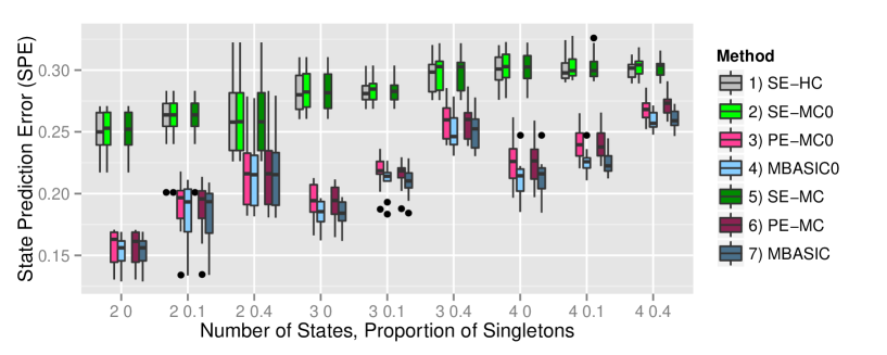
Figure B.3: Simulation Study 1, negative binomial distribution. Boxplots for ARI, MSE-W, and SPE across 10 simulated datasets. The number of states is varied at 2, 3, and 4, and the proportion of singletons at 0, 0.1, 0.4. Table B.1 summarizes the methods compared.

Figure B.4: Simulation study 1, binomial distribution. Boxplots for ARI, MSE-W, and SPE across 10 simulated datasets. The number of states is varied at 2, 3, and 4, and the proportion of singletons at 0, 0.1, 0.4. Table B.1 summarizes the methods compared.

We utilized several criteria to compare the performance of MBASIC to the benchmark algorithms in Table B.1. To estimate how well the state space was characterized for each cluster, we computed the mean-squared error for $W$ (MSE-W) as MSE-W=$\sqrt{\sum_{j,k,s}(\hat{w}_{jks}-w_{jks})^{2}/(JKS)}$ . We also evaluated how well each method recovered the true state variables $\theta_{ik}$’s. This was reflected by the state prediction error (SPE) as the mean squared error between the simulated states $\theta_{ik}$’s and their posterior probabilities: SPE=$\sqrt{\sum_{i,k,s}[1\{\theta_{ik}=s\}-P(\theta_{ik}=s|Y)]^{2}/(IKS)}$. Finally, to compare the estimated clustering with the simulated true clustering, we computed the Adjusted Rand Index (ARI) (Rand, 1971). ARI is a measure for the similarity between two different clusterings of the data. Its value ranges between -1 and 1, with 1 indicating perfect match between the two clusterings.

ARI requires the true clusters denoted by $\mathscr{C}_{j},~{}0\leq j\leq J$ and their estimates denoted by $\hat{\mathscr{C}}_{j},~{}0\leq j\leq\hat{J}$. In our simulations, they were computed as:

$$\mathscr{C}_{0}=\{1\leq i\leq I:b_{i}=1\};~{}\mathscr{C}_{j}=\{1\leq i\leq I:b_{i}=0,~{}z_{ij}=1\},~{}j\leq 1,$$

where $\mathscr{C}_{0}$ denoted the set of singleton units. $\hat{\mathscr{C}}_{j}$ was computed from the posterior distributions as $\hat{\mathscr{C}}_{j}=\{1\leq i\leq I:j=\arg\max_{0\leq j\leq J}P(i\in\mathscr{C}_{j}|Y)\}$, where $P(i\in\mathscr{C}_{0}|Y)=E(b_{i}|Y)$, and $P(i\in\mathscr{C}_{j}|Y)=E[(1-b_{i})z_{ij}|Y]$.

The simulation results under various settings are summarized by the boxplots for each criterion in Figures B.2, B.3, and B.4. Across all different simulation settings, the performance of MBASIC was consistently among the best in all of the ARI, MSE-W, and SPE metrics. This shows that MBASIC could not only recover the clustering structure, but also achieve high accuracy in estimating individual states. SE-HC, SE-MC and SE-MC0 performed the worst in both detecting the clustering structure and estimating the individual states. This suggests that separating state-space inference from joint model fitting can significantly deteriorate model estimation. Different from the SE-* methods, performances of PE-MC and PE-MC0 were much closer to MBASIC. For the negative binomial and binomial distributions (Figures B.3 and B.4), PE-MC achieved similar ARI levels to MBASIC and slightly larger SPE values. These observations show that by jointly estimating the clusters and the states, data under different conditions could borrow information from each other and thus substantially improve the state-space estimation. Overall, these observations are consistent with the results in Wei et al. (2015) and Wei et al. (2012).

The simulation results also highlight the effect of modeling the singleton cluster in various settings. Comparing the performances of MBASIC with MBASIC0 and PE-MC with PE-MC0, we see that modeling the singleton cluster does not have a significant effect when the proportion of singletons is low, i.e., $\zeta=0$ or $0.1$; however, the improvement is highly significant when $\zeta=0.4$. When $\zeta=0.4$, including singletons significantly improved the performance with respect to ARI, but did not have an obvious effect on SPE. This has several implications in practice. First, the fact that MBASIC does not under-perform any other methods when $\zeta=0$ or $0.1$ indicates that increasing the model complexity by introducing singletons does not lead to unrobust inference. Because we are always agnostic on the existence of singletons for any real data, keeping them in our model would guard against their adverse influence in inferring the clustering structure. Second, although incorporating the singleton cluster does not improve estimating individual states, some epigenetic studies focus primarily on the association structure between units, as our example in 4.2. For such studies, the gain in estimating the clustering structure by including the singletons is essential. We note that in the comparison of SE-MC0 with SE-MC for the negative binomial and the binomial distributions (Figures B.3 and B.4), modeling the singletons does not necessarily improve estimation for separate model fitting even when the proportion of singletons is high, e.g., $\zeta=0.4$. This might suggest that the state-space estimation step is introducing additional noise to the clustering step, which in turn makes it less favorable to infer a complicated clustering structure with singletons.

B.2 Simulation Study 2: Model Selection

Table B.2: Simulation study 2, Scenario 1, unstructured clusters. Simulation results for model selection without structural constraints. For each criterion, the mean is computed over 10 simulated data sets, with the standard deviation shown in the parentheses.

Dist.	$\zeta$	$J$	ARI	MSE-W	SPE
Bin	0.1	20.8 ( 2.098 )	0.94 ( 0.036 )	0.096 ( 0.018 )	0.159 ( 0.014 )
Bin	0.4	20.9 ( 1.101 )	0.914 ( 0.035 )	0.122 ( 0.034 )	0.204 ( 0.012 )
LN	0.1	20.7 ( 0.823 )	0.989 ( 0.005 )	0.044 ( 0.03 )	0.086 ( 0.006 )
LN	0.4	21.3 ( 1.337 )	0.972 ( 0.007 )	0.095 ( 0.027 )	0.107 ( 0.008 )
NB	0.1	21.6 ( 0.843 )	0.947 ( 0.021 )	0.089 ( 0.028 )	0.154 ( 0.007 )
NB	0.4	20.6 ( 2.271 )	0.902 ( 0.026 )	0.112 ( 0.048 )	0.189 ( 0.007 )

Table B.3: Simulation study 2, Scenario 2, structured clusters. Simulation results for model selection with structural constraints. For each criterion, the mean is computed over 10 simulated data sets, with the standard deviation shown in the parentheses.

Dist.	$\zeta$	$J_{1}$	$J$	ARI	MSE-W	SPE
Bin	0.1	10.3 ( 1.16 )	20.7 ( 1.494 )	0.934 ( 0.022 )	0.084 ( 0.035 )	0.162 ( 0.02 )
Bin	0.4	10.3 ( 1.636 )	21 ( 2.625 )	0.897 ( 0.048 )	0.125 ( 0.03 )	0.196 ( 0.031 )
LN	0.1	10.4 ( 0.516 )	20.6 ( 0.516 )	0.984 ( 0.015 )	0.044 ( 0.032 )	0.086 ( 0.006 )
LN	0.4	11.2 ( 1.619 )	22.5 ( 1.509 )	0.968 ( 0.01 )	0.108 ( 0.037 )	0.106 ( 0.006 )
NB	0.1	10.9 ( 1.197 )	21 ( 1.054 )	0.955 ( 0.019 )	0.064 ( 0.035 )	0.155 ( 0.008 )
NB	0.4	11.2 ( 1.814 )	22.2 ( 1.398 )	0.926 ( 0.014 )	0.108 ( 0.031 )	0.184 ( 0.013 )

This second set of simulations aimed to evaluate the use of BIC to select the number of clusters as well as the structural constraints for each cluster. We simulated data sets under two scenarios. For the first scenario, each data set had $J=20$ clusters with $K=30$ experimental conditions, and none of the clusters had structural constraints. For the second scenario, each data set had $J=20$ clusters over $K=30$ conditions, but $J_{1}=10$ of the clusters were structurally constrained as follows:

$$w_{j,k,s}=w_{j,k+K/2,s},\forall j,1\leq j\leq J/2;\forall k,1\leq k\leq K/2.$$

We refer the two scenarios as the unstructured scenario and the structured scenario, respectively. We considered log-normal distributions (3), negative binomial distributions (4) and binomial distributions (5) for both cases. We also varied the proportion of singleton units $\zeta$ at 0.1 and 0.4. The number of states was fixed at $S=2$. The remaining parameters were simulated following the same mechanism as in Section B.1.1.

For each simulated data set, we fitted a number of candidate models. For the unstructured scenario, we varied the number of clusters $J$ from 10 to 30. For the structured scenario, we followed the two-phase procedure described in Section 3.4 of our main article. The best model was selected by the minimum BIC value. To assess the performances of these selected models, we computed the ARI, MSE-W and SPE metrics as described in Section B.1.

The simulation results are summarized in Tables B.2 and B.3. Under each set of parameters, we computed the mean and the standard deviation for each of the criterion as well as the selected value of $J$ and $J_{1}$ under 10 simulated data sets. These tables show that the selected values for $J$ and $J_{1}$ were very close to the true values. Moreover, MBASIC performed uniformly well with respect to ARI, MSE-W, and SPE under different settings. These results indicate that even if MBASIC may not identify the “true” structure that drives the actual data, the identified structures can still properly represent the state-space associations between units.

B.3 Simulation Studies 3-5: Comparison with iASeq and CorMotif

In this section, we compare MBASIC with two recently proposed models for integrative analysis of specific types of genomic data: CorMotif (Wei et al., 2015) and iASeq (Wei et al., 2012). Both models have the similar state-space clustering structure as MBASIC. The main difference from MBASIC is that they each incorporate more complicated distributional assumptions targeting specific genomic data types. The CorMotif model specifically addresses integrative differential expression analysis with $n_{k1}$ case condition replicates and $n_{k0}$ control condition replicates for each experimental condition $k$. It inherits the LIMMA (Smyth, 2004) framework for differential analysis of gene-expression data and assumes mixture of Gaussian distributions with $S=2$ states: $s=1$ for the equally expressed state, and $s=2$ for the differentially expressed state. Specifically, the CorMotif model has the following state-space mapping structure:

$$\frac{n_{k}s_{k}^{2}}{\sigma_{ik}^{2}}\sim \chi_{n_{k}}^{2},$$

$$\mu_{ik}|\sigma_{ik}^{2}\sim N(0,u_{k}\sigma_{ik}^{2}),$$

$$(Y_{ikl}|\theta_{ik}=1)\sim N(\mu_{ik0},\sigma_{ik}^{2}),~{}l=1,2,\cdots,n_{k1},$$

$$(Y_{ikl}|\theta_{ik}=2)\sim N(\mu_{ik0}+\mu_{ik},\sigma_{ik}^{2}),~{}l=1,2,\cdots,n_{k1},$$

$$X_{ikl}\sim N(\mu_{ik0},\sigma_{ik}^{2}),~{}l=1,2,\cdots,n_{k0},$$

where $X_{ikl}$’s are the observed data from control experiments, and $Y_{ikl}$ are the observed data from the case experiments. $n_{k}$ and $s_{k}^{2}$ are hyper parameters specific to each experiment to account for potential heterogeneity among units within the same state, and $u_{k}$ reflects the strength of differential expression. CorMotif assumes almost the same state-space clustering structure as MBASIC except that it does not include singletons. The iASeq model, targeting at allele-specific binding problems has the following state-space mapping structure:

$$Y_{ikl}\sim Binom(\gamma_{ikl},p_{ik}),$$

$$p_{ik}|\theta_{ik}=2\sim Beta(\alpha_{k},\beta_{k}),$$

$$p_{ik}|\theta_{ik}=1\sim Unif\left(0,\frac{\alpha_{k}}{\alpha_{k}+\beta_{k}}\right),$$

$$p_{ik}|\theta_{ik}=3\sim Unif\left(\frac{\alpha_{k}}{\alpha_{k}+\beta_{k}},1\right),$$

where the $\alpha_{k}$, $\beta_{k}$ are experiment-specific parameters, and $\gamma_{ikl}$ is the observed total number of reads between two alleles. The state-space mapping structure for iASeq is almost the same as MBASIC, except that it assumes no singletons, and that one cluster is dedicated to equal binding/occupancy between the alleles (i.e., $w_{1k1}=1,~{}\forall 1\leq k\leq K$).

There are two key differences between CorMotif/iASeq and MBASIC. First, both CorMotif and iASeq address the heterogeneity among the units within the same state, and they introduce additional hyper parameters to model the heterogeneous parameters associated with the distribution of individual units. Compared to MBASIC, where we assume the distributions within the same state are homogeneous, such heterogeneous distributional assumptions are much more realistic. Second, CorMotif and iASeq implement two-stage estimation procedures similar to PE-MC0, which separate parameter estimation from state-space clustering. Wei et al. (2015) pointed out that once we have the heterogeneous distributional parameters within each state, joint model fitting for all parameters would require running a Markov Chain Monte-Carlo algorithm rather than the simple E-M algorithm we have developed for MBASIC. Therefore, the computational cost ensued might render its applicability for large real data sets.

In comparison of MBASIC to CorMotif and iASeq, we simulated data according to each of the assumed distributions of CorMotif/iASeq, but fitted MBASIC models using simplified distributions. For data simulated from the iASeq model, we used MBASIC to fit binomial distributions with $S=3$ states (5). For data simulated from the CorMotif model, we first generated two versions of t-statistics as follows. For each unit and experiment, denote $\overline{Y}_{ik}=\sum_{l=1}^{n_{k1}}Y_{ikl}/n_{k1}$, $\overline{X}_{ik}=\sum_{l=1}^{n_{k0}}X_{ikl}/n_{k0}$, $\tilde{s}_{ik}^{2}=[\sum_{l=1}^{n_{k1}}(Y_{ikl}-\overline{Y}_{ik})^{2}+\sum_{l=1}^{n_{k0}}(X_{ikl}-\overline{X}_{ik})^{2}]/(n_{k1}+n_{k0}-2)$ and $v_{k}=1/n_{k1}+1/n_{k0}$. We computed the naive t-statistic $T_{ik}$ as:

$$T_{ik}=\frac{\overline{Y}_{ik}-\overline{X}_{ik}}{\sqrt{v_{k}}\tilde{s}_{k}}.$$ (47)

We also computed the limma t-statistic $\tilde{T}_{ik}$ by first fitting the data for each condition using LIMMA (Smyth, 2004) to estimate $n_{k}$ and $s_{k}^{2}$, then computed:

$$\tilde{T}_{ik}=\frac{\sqrt{n_{k}+n_{k1}+n_{k0}-2}(\overline{Y}_{ik}-\overline{X}_{ik})}{\sqrt{v_{k}[(n_{k1}+n_{k0}-2)\tilde{s}_{k}^{2}+n_{k}s_{k}^{2}]}}.$$ (48)

For each set of $T_{ik}$’s and $\tilde{T}_{ik}$’s, we fitted the MBASIC model with $S=2$ components of scaled-t distributions:

$$T/\mu_{ks}|\theta_{iks}=1~{}\sim~{}t_{\sigma_{ks}},~{}~{}s=1,~{}2.$$ (49)

Here, $\mu_{ks}$ is the scaling parameter, and $\sigma_{ks}$ is the degrees of freedom. Because we pooled the replicate level data to generate these t-statistics, the parameters $\mu$ and $\sigma$ no longer depended on $l$. We refer to the method using $\tilde{T}_{ik}$ as MBASIC-limma, and using $T_{ik}$ as MBASIC-t. Because there is no closed form maximum likelihood solution for t-distributions, we use the moment method to estimate $\mu_{ks}$’s and $\sigma_{ks}$’s in the M-step similar to the case of negative binomial distributions.

Table B.4: Summary for the designs of the simulation settings in Simulation Study 4, originally designed by Wei et al. (2015).

Simulation Setting	$I$	$J$	$K$
1	10,000	4	4
2	10,000	4	4
3	10,000	5	8
4	10,000	5	20

In Simulation Study 3, we simulated data following the iASeq model. We set $\alpha_{k}=\beta_{k}=2$, and simulated state-space variables the same as in Section B.1 with $I=4000$. We set $J=10,~{}20$ and $\zeta=0,~{}0.1,~{}0.4$. Simulation Studies 4-5 compare MBASIC with CorMotif. In Simulation Study 4, we simulated data in four settings corresponding to Simulations 1-4 of Wei et al. (2015) respectively. In these settings, we had $n_{k}=4$, $u_{k}=4$, $s_{k}^{2}=0.02$. Table B.4 summarizes the settings for the number of clusters, experiment conditions, and units for the state-space variables. We refer our readers to Wei et al. (2015) for more details of the state-space design. We note that Wei et al. (2015) simulations did not include singletons (i.e., $\zeta=0$) and furthermore, their settings assumed $w_{jks}\in\{0,~{}1\}$. This means that the state-space variables are completely determined by the clustering structure. In Simulation Study 5, we set $n_{k}$ and $s_{k}^{2}$ the same as in Simulation Study 4, but varied $u_{k}$ as $u_{k}=8$ for easier distinction between different states. However, we simulated $w_{jks}$ following S-dimensional Dirichlet distributions as in Simulation Study 1 to introduce noises in generating state-space variables. In addition, we simulated data with smaller number of units ($I=4000$), but more clusters ($J=10,~{}20$), and varied the proportion of singletons $\zeta=0,~{}0.1,~{}0.4$. The other details of generating state-space variables were the same as in Section B.1.

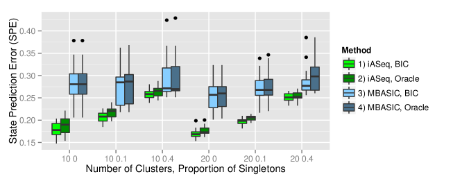
Figure B.5: Simulation Study 3, comparison between MBASIC and iASeq. We varied the number of clusters at 10, 20 and the proportion of singletons at 0, 0.1 and 0.4. Results are summarized over 10 simulations under each setting.

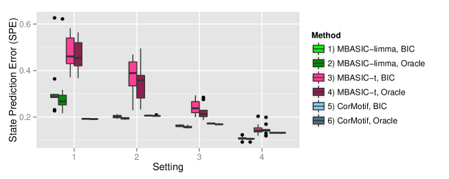
Figure B.6: Simulation Study 4, comparison between MBASIC and CorMotif. We simulated data under four settings as in Table B.4. Results are summarized over 10 simulations under each setting.

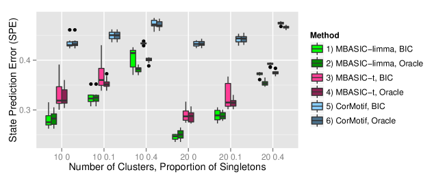
Figure B.7: Simulation Study 5, comparison between MBASIC and CorMotif. We varied the number of clusters at 10, 20 and the proportion of singletons at 0, 0.1 and 0.4. Results are summarized over 10 simulations under each setting.

Simulation Study 4, Setting 1	Simulation Study 4, Setting 2
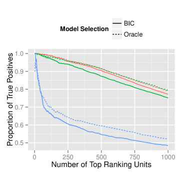
Simulation Study 4, Setting 3	Simulation Study 4, Setting 4

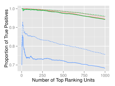
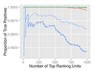
Figure B.8: Simulation Study 4, comparison between MBASIC and CorMotif. The average true positive rate for the 10 simulations among the 1000 highest ranking unit-experiment pairs for each of the four simulation settings in Table B.4. For each simulation, the “true positive” set consists of $(i,~{}k)$’s with $\theta_{ik}=2$, and the ranking is based on the posterior probability $P(\theta_{ik}=2|Y)$.

Table B.5: Simulation Studies 3-5. A summary of the simulation designs, the fitting algorithms compared, and the figure numbers for the results.

Study	$J$	$\zeta$	True model	Fitting algorithms	Related figures
3	10, 20	0, 0.1, 0.4	iASeq	MBASIC, iASeq	Figure B.5
4	4, 5	0	CorMotif	MBASIC-limma, MBASIC-t, CorMotif	Figures B.6, B.8
5	10, 20	0, 0.1, 0.4	CorMotif	MBASIC-limma, MBASIC-t, CorMotif	Figure B.7

Table B.5 further summarizes the components of the Simulation Studies. For each set of parameters, we simulated 10 data sets. We computed ARI, MSE-W, and SPE based on both the model with the number of clusters selected by BIC, and the oracle model where the number of clusters is set to its true value. The comparison between MBASIC and iASeq is shown in Figure B.5. For all the different settings, MBASIC achieved better clustering performance, with higher ARI values. However, iASeq performed better in SPE and MSE-W. When $\zeta=0$, iASeq performed overall better than MBASIC, with similar ARI values as MBASIC but much lower SPE. However, as $\zeta$ increased, iASeq’s ARI value became significantly smaller than MBASIC, while its SPE value became closer to MBASIC’s. In such cases, the benefits of modeling singletons seem to outweigh the loss of using simplified distributional assumptions.

The comparison between MBASIC and CorMotif is summarized in Figures B.6 and B.7. In Simulation Study 4 (Figure B.6), because CorMotif models did not allow singletons, we also excluded the singleton cluster in fitting MBASIC models. MBASIC-limma performed the best except in the first setting, where CorMotif achieved the best SPE. Figure B.8 depicts the average true positive rate in detecting states with $\theta_{ik}=2$ among the 1000 top ranking units for each of the four settings. In all but Setting 1, MBASIC-limma performed equally well as CorMotif. We note that Setting 1 has the fewest clusters $J=4$ and the fewest experimental conditions $K=4$, while the other settings have more complicated state-space structures. Performance of MBASIC-t was the worst in all the four settings. This suggests that neglecting the heterogeneity in these cases can significantly increase estimation error. Although MBASIC model alone does not address the heterogeneity issue, fitting MBASIC models after a data pre-processing step that incorporates the heterogeneity structure, such as computing $\tilde{T}_{ik}$ in MBASIC-limma, can significantly improve model inference. In Simulation Study 5 where we had stronger signals in separating distribution components but noisy state-space clusters, CorMotif resulted in the largest SPE values in all settings (Figure B.7). Although its performance in ARI was comparable with MBASIC-limma when $\zeta\leq 0.1$, it deteriorated with increasing proportion of singletons, i.e., $\zeta=0.4$. Simulation Studies 4 and 5 collectively suggest that MBASIC’s performance is competitive with CorMotif in settings where we have less noise in clustering structure, small numbers of clusters, and some level of singletons despite the fact that the distributional assumptions of MBASIC might be mis-specified. This indicates that for real data sets where we are agnostic about the true data generating structure, MBASIC might be a more general and robust approach.

B.4 Simulation Study 6: Weak Clusters

Wei et al. (2015) pointed out that state-space clustering without accommodating singletons can lead to merging of small clusters with large clusters with distinct state-space profiles. Such a phenomenon may alter the interpretation of the $W$ matrix, because each column may represent the average state-space pattern of several small clusters that lack the data support. It is therefore important to investigate whether such a phenomenon still exists for MBASIC where we include a singleton cluster.

(a) Simulations 1-3	(b) Simulations 4-6

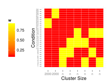
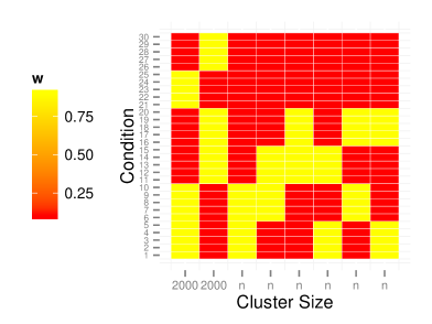
Figure B.9: Simulation Study 6. Two settings of the true cluster patterns, represented by the matrix $(w_{jk2})_{1\leq j\leq 8,~{}1\leq k\leq 30}^{T}$.

We conducted six simulations in Simulation Study 6 to investigate this issue. We simulated data according to the log-normal distribution with $S=2$ states, $J=8$ clusters, and $K=30$ conditions. The number of replicates within each condition, as well as the distribution parameters within each state is the same as in Section B.1.1. We set the sizes of the first two clusters as 2000, and varied the size of each of the other six clusters, that is $n_{\textnormal{small}}$, as 20 or 100. To vary the level of state-space similarity between the two big clusters and the small clusters, we had two settings for the state-space pattern as shown in Figure B.9. For Simulations 1-3, the conditions in which the small clusters have state $s=2$ are distinct from the two big clusters, while for Simulations 4-6, the patterns between the small and large clusters are more similar. To control these cluster patterns, we set $w_{jks}\in\{0.1,~{}0.9\}$. Finally, we included $n_{\textnormal{singleton}}=$ 0 or 2000 singletons in each simulated data set. The states for the singleton units were generated the same as in Section B.1.1.

	(a) MBASIC	(b) MBASIC0
$n_{\textnormal{small}}=20$ $n_{\textnormal{singleton}}=0$
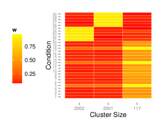
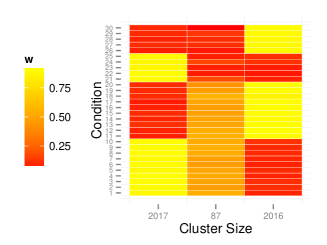
	(c) MBASIC	(d) MBASIC0
$n_{\textnormal{small}}=20$ $n_{\textnormal{singleton}}=2000$
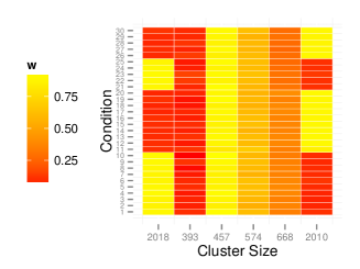
	(e) MBASIC	(f) MBASIC0
$n_{\textnormal{small}}=100$ $n_{\textnormal{singleton}}=0$

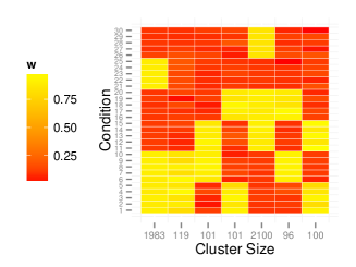
Figure B.10: Simulation Study 6, Simulations 1-3. Estimated cluster patterns by (a, c, e) MBASIC and (b, d, f) MBASIC0. The true clustering pattern is shown in Figure B.9(a).

	(a) MBASIC	(b) MBASIC0
$n_{\textnormal{small}}=20$ $n_{\textnormal{singleton}}=0$
	(c) MBASIC	(d) MBASIC0
$n_{\textnormal{small}}=20$ $n_{\textnormal{singleton}}=2000$
	(e) MBASIC	(f) MBASIC0
$n_{\textnormal{small}}=100$ $n_{\textnormal{singleton}}=0$

Figure B.11: Simulation Study 6, Simulations 4-6. Estimated cluster patterns by (a, c, e) MBASIC and (b, d, f) MBASIC0. The true clustering pattern is shown in Figure B.9(b).

Table B.6: Simulation Study 6, Simulations 1-3. Confusion matrix between the true clusters and the estimated clusters. The true cluster pattern is shown in Figure B.9(a).

Simulation 1, $n_{\textnormal{small}}=20$, $n_{\textnormal{singleton}}=0$
MBASIC True 0 1 2 1 23 2 1975 2 30 1967 3 3 20 0 0 4 20 0 0 5 20 0 0 6 20 0 0 7 20 0 0 8 20 0 0	MBASIC0 True 1 2 3 1 1998 2 0 2 4 1995 1 3 0 1 19 4 0 1 19 5 0 0 20 6 0 1 19 7 0 0 20 8 0 1 19
Simulation 2, $n_{\textnormal{small}}=20$, $n_{\textnormal{singleton}}=2000$
MBASIC True 0 1 2 3 0 1957 19 17 7 1 180 1818 2 0 2 153 3 1844 0 3 20 0 0 0 4 20 0 0 0 5 20 0 0 0 6 20 0 0 0 7 20 0 0 0 8 20 0 0 0	MBASIC0 True 1 2 3 4 5 6 0 67 372 620 59 427 455 1 1957 25 0 4 0 14 2 8 23 3 1950 0 16 3 0 0 1 0 0 19 4 0 0 0 0 0 20 5 0 0 1 0 0 19 6 0 0 1 0 0 19 7 0 0 1 0 0 19 8 0 0 1 0 0 19
Simulation 3, $n_{\textnormal{small}}=100$, $n_{\textnormal{singleton}}=0$
MBASIC True 0 1 2 3 4 5 1 21 1974 0 0 5 0 2 12 7 0 1 1980 0 3 1 1 9 0 0 89 4 5 0 89 0 0 6 5 6 0 2 92 0 0 6 1 0 0 13 0 86 7 0 0 96 4 0 0 8 0 0 0 97 0 3	MBASIC0 True 1 2 3 4 1 1993 0 7 0 2 7 1 1991 1 3 1 0 0 99 4 0 2 0 98 5 0 99 0 1 6 0 6 0 94 7 0 100 0 0 8 0 99 0 1

Table B.7: Simulation Study 6, Simulations 4-6. Confusion matrix between the true clusters and the estimated clusters. The true cluster pattern is shown in Figure B.9(b).

Simulation 4, $n_{\textnormal{small}}=20$, $n_{\textnormal{singleton}}=0$
MBASIC True 0 1 2 1 5 1995 0 2 1 0 1999 3 1 19 0 4 19 1 0 5 1 0 19 6 20 0 0 7 18 1 1 8 20 0 0	MBASIC0 True 1 2 3 1 1999 1 0 2 0 0 2000 3 17 3 0 4 0 20 0 5 0 5 15 6 0 20 0 7 0 19 1 8 1 19 0
Simulation 5, $n_{\textnormal{small}}=20$, $n_{\textnormal{singleton}}=2000$
MBASIC True 0 1 2 0 1986 7 7 1 31 1969 0 2 45 0 1955 3 11 9 0 4 20 0 0 5 8 0 12 6 20 0 0 7 20 0 0 8 20 0 0	MBASIC0 True 1 2 3 4 5 6 0 16 393 457 561 560 13 1 1990 0 0 5 5 0 2 0 0 0 5 12 1983 3 12 0 0 1 7 0 4 0 0 0 1 19 0 5 0 0 0 0 6 14 6 0 0 0 0 20 0 7 0 0 0 0 20 0 8 0 0 0 1 19 0
Simulation 6, $n_{\textnormal{small}}=100$, $n_{\textnormal{singleton}}=0$
MBASIC True 0 1 2 3 4 5 6 7 1 3 1983 14 0 0 0 0 0 2 1 0 0 0 0 1999 0 0 3 0 8 92 0 0 0 0 0 4 1 0 0 1 98 0 0 0 5 1 0 0 0 0 99 0 0 6 1 0 0 0 0 0 99 0 7 1 0 1 96 0 1 0 1 8 0 0 0 0 0 0 0 100	MBASIC0 True 1 2 3 4 5 6 7 1 1976 24 0 0 0 0 0 2 0 0 0 0 2000 0 0 3 7 93 0 0 0 0 0 4 0 0 99 0 0 1 0 5 0 0 0 0 99 0 1 6 0 0 1 0 0 0 99 7 0 2 1 1 1 95 0 8 0 0 0 100 0 0 0

Table B.8: Simulation Study 6. ARI, MSE-W, and SPE in all simulations.

			MBASIC			MBASIC0
Simulation	$n_{\textnormal{small}}$	$n_{\textnormal{singleton}}$	ARI	MSE-W	SPE	ARI	MSE-W	SPE
1	20	0	0.967	0.433	0.185	0.991	0.29	0.189
2	20	2000	0.79	0.442	0.192	0.727	0.34	0.193
3	100	0	0.969	0.203	0.187	0.975	0.233	0.193
4	20	0	0.977	0.384	0.169	0.983	0.260	0.167
5	20	2000	0.926	0.384	0.185	0.773	0.333	0.184
6	100	0	0.949	0.087	0.172	0.947	0.087	0.171

In each simulation, we fitted the data using MBASIC and MBASIC0 with BIC to select the number of clusters. MBASIC0 differs from MBASIC only by the exclusion of the singleton feature. Therefore, comparing these two methods allow us to assess how fitting a singleton cluster may affect the small cluster merging problem. Tables B.6 and B.7 compare the confusion matrices between the fitted and the true clusters. We also display the state-space patterns of the fitted models in Figures B.10 and B.11. In Simulations 1 and 4, with $n_{\textnormal{small}}=20$ units in each of the small clusters, MBASIC classified the units of small clusters as singletons, while MBASIC0 merged them to form a spurious cluster. The state-space pattern estimated by MBASIC represented the two real big clusters. When the data included singletons, as in Simulations 2 and 5, MBASIC0 formed more spurious clusters, while MBASIC continued to allocate the small clusters as singletons. When we had $n_{\textnormal{small}}=100$ units in each of the small clusters, both methods identified these small cluster patterns in Simulation 6 (Figure B.11), but formed spurious clusters in Simulation 3 (Figure B.10). We compare the resulting ARI, MSE-W, and SPE between MBASIC and MBASIC0 in Table B.8. Performances of these two methods are close when we have no singletons, but differentiate otherwise. Based on these simulations, we conclude that fitting a singleton cluster can substantially avoid merging weak clusters. The state-space patterns estimated by the $W$ matrix are more likely to reflect true underlying clusters rather than the average of several small clusters. We acknowledge that how well modeling the singletons can avoid merging weak clusters requires further investigation in more dynamic settings as we vary the similarity among clusters, the difference among the states, as well as other variables that influence cluster structures such as $J$, $K$, $S$. We leave such potential investigations as future research.

Appendix C Additional Tables and Figures

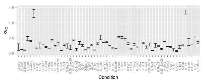
Figure C.12: The range of the estimated parameters $\mu_{kls}$ and $\sigma_{kls}$ among the different replicates under the same experimental condition for the transcription factor enrichment network data in Section 4.1.

(a)	(b)

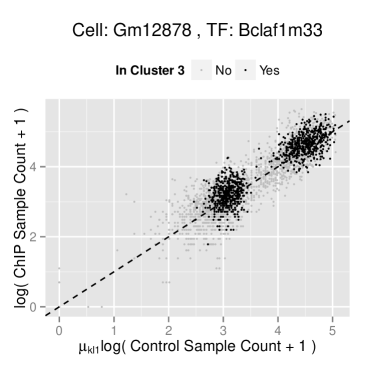
Figure C.13: Plots of the transformed ChIP sample read counts against the transformed control sample read counts for all units in the Gm12878 cell for (a) Bcl3 and (b) Bclaf1. Data from unenriched units are expected to locate around the 45 degree dashed line.

(a)	(b)

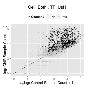
Figure C.14: Plots of the transformed ChIP sample read counts against the transformed control sample read counts for all units in both Gm12878 and K562 cells for (a) Max and (b) Usf1. Data from unenriched units are expected to locate around the 45 degree dashed line.

Table C.9: Enriched cell type-TF combination for each cluster in the TF enrichment network analysis of Section 4.1 of the main text. TFs with estimated enrichment probability $>95\%$ are listed for each cluster.

Cluster	# of Loci	Common TF	Gm12878 Specific	K562 Specific
1	34	Bcl3, Max, Sp1, Taf1, Zbtb33	Atf3, Ets1, Jund, Nrf1, Pol24h8, Sin3ak20, Tr4	Egr1, Pu1, Rad21, Usf2
2	317	Bcl3, Chd2, Max, Pol24h8, Sp1, Taf1	Atf3, Ets1, Nrf1, Sin3ak20, Usf2	Bclaf1, Egr1, Pu1, Smc3, Tbp, Zbtb33
3	490	Ets1, Pol2, Pol24h8, Sin3ak20, Taf1, Tbp, Usf1	Atf3, Chd2, Nrf1, Usf2	Bcl3, Bclaf1, Max, Sp1
4	555	Bcl3, Bclaf1, Chd2, Pol2, Pol24h8, Sp1, Taf1, Tbp	Atf3, Ets1, Nrf1, Sin3ak20, Six5, Smc3	Pu1
5	428	Bcl3, Chd2, Ets1, Pol24h8, Sp1, Taf1	Atf3, Ctcf, Nrf1, Rad21, Sin3ak20	Bclaf1, Pol2, Smc3, Tbp
6	729	Bcl3, Chd2, Ets1, Pol2, Pol24h8, Sin3ak20, Smc3, Sp1, Taf1	Atf3, Nrf1	Bclaf1, Egr1, Tbp
7	391			Bcl3, Bclaf1, Chd2, Egr1, Ets1, Smc3, Sp1
8	133	Ctcf	Atf3, Chd2, Rad21	Smc3, Srf
9	146	Ctcf		Bclaf1, Pol24h8, Smc3, Tbp
10	469	Pol2, Pol24h8, Taf1	Smc3	Bclaf1, Ets1, Sin3ak20, Tbp
11	440	Gabp, Pol24h8, Taf1	Ets1, Smc3	Pol2
12	184		Bcl3, Chd2, Ets1, Nrf1, Pol24h8, Taf1
13	277	Chd2, Pol2, Pol24h8, Sp1, Taf1, Tbp	Smc3	Cfos
14	156	Chd2, Pol2, Pol24h8, Tbp, Zbtb33	Ets1, Smc3, Taf1
15	412	Pol2, Pol24h8
16	327		Pol24h8
17	213	Usf1	Atf3, Usf2	Max
18	241	Six5	Ets1, Smc3
19	187	Chd2, Sp1		Cfos
20	222			Ets1
21	385			Pol24h8
22	343	Ctcf		Smc3
23	449		Nrf1, Smc3
24	1674

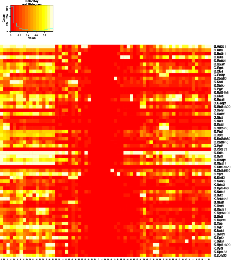
Figure C.15: Estimated enrichment probability for each of the 90 clusters identified by MClust.

Figure C.16: The range of the estimated parameters $\mu_{kls}$ among the different replicates under the same experimental condition for the +9.5 composite element data in Section 4.2.

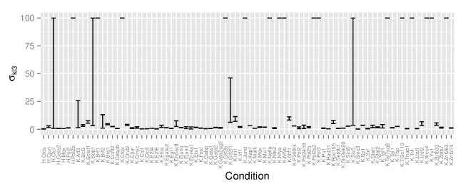
Figure C.17: The range of the estimated parameters $\sigma_{kls}$ among the different replicates under the same experimental condition for the +9.5 composite element data in Section 4.2. For a subset of the replicates, the data for an individual state can be under-dispersed, resulting in a negative value for the estimated size parameter in the negative binomial distribution. In that case, we set $\sigma_{kls}=100$. Although our model do not fully capture the under-dispersion patterns, the large variations in $\sigma_{kls}$ for a subset of the experimental conditions suggest that assuming replicate-specific distributions is quite necessary.

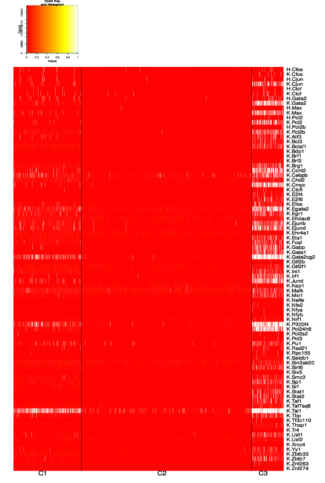
Figure C.18: Enrichment states provided by the ENCODE peak profiles. Seven empty rows corresponding to the TFs that lack ENCODE peak profiles. Note that only a small percentage of the composite elements which harbor the canonical GATA binding site are identified as enriched for GATA family transcription factors. This suggests that the ENCODE peak profiles can be conservative.

(a)	(b)

Figure C.19: (a, b) ChIP sample read counts against control sample read counts for one replicate with K562-Yy1. Enrichment status are annotated by (a) the ENCODE peak profiles and (b) MBASIC prediction.

Table C.10: Annotations for +9.5 Element-like loci in 5p1 (2Kb upstream of transcription start site (TSS)), 5p2 (2Kb to 10Kb upstream of TSS) and intronic regions.

Ref ID	Gene	Chr	Strand	Gene Start	Gene End	Region	Distance	Peak Start	Peak End	+9.5 Similarity
NM_001145662	GATA2	chr3	-	128198264	128206764	intron	4601	128202079	128202248	0.964
NM_001145661	GATA2	chr3	-	128198264	128207373	intron	5210	128202079	128202248	0.964
NM_032638	GATA2	chr3	-	128198264	128212030	intron	9867	128202079	128202248	0.964
NM_005225	E2F1	chr20	-	32263292	32274210	5p2	-3886	32278012	32278182	0.774
NM_001166	BIRC2	chr11	+	102217965	102249394	5p2	-5004	102212877	102213046	0.753
NM_203343	EPB41	chr1	+	29213602	29446558	intron	39968	29253487	29253655	0.74
NM_203342	EPB41	chr1	+	29213602	29446558	intron	39968	29253487	29253655	0.74
NM_001166007	EPB41	chr1	+	29213602	29446558	intron	39968	29253487	29253655	0.74
NM_004437	EPB41	chr1	+	29213602	29446558	intron	39968	29253487	29253655	0.74
NM_001166005	EPB41	chr1	+	29213602	29446558	intron	39968	29253487	29253655	0.74
NM_001166006	EPB41	chr1	+	29241087	29391731	intron	12483	29253487	29253655	0.74
NM_173485	TSHZ2	chr20	+	51588876	52103965	intron	203292	51792084	51792253	0.735
NM_007077	AP4S1	chr14	+	31494682	31555007	intron	13234	31507832	31508001	0.733
NM_001128126	AP4S1	chr14	+	31494682	31562634	intron	13234	31507832	31508001	0.733
NM_001430	EPAS1	chr2	+	46524540	46613842	intron	42757	46567214	46567382	0.728
NM_018119	POLR3E	chr16	+	22308740	22345341	intron	833	22309489	22309658	0.719
NM_181442	ADNP	chr20	-	49506882	49547527	intron	27423	49520020	49520189	0.718
NM_015339	ADNP	chr20	-	49506882	49547527	intron	27423	49520020	49520189	0.718
NM_020359	PLSCR2	chr3	-	146151081	146213722	5p1	-921	146214559	146214728	0.718
NM_006257	PRKCQ	chr10	-	6469104	6622238	intron	106706	6515449	6515617	0.713
NM_018309	TBC1D23	chr3	+	99979685	100044078	intron	28727	100008329	100008497	0.711
NM_020382	SETD8	chr12	+	123868703	123893898	intron	4170	123872789	123872958	0.71
NM_015385	SORBS1	chr10	-	97071530	97321171	intron	29191	97291896	97292065	0.709
NM_024991	SORBS1	chr10	-	97071530	97321171	intron	29191	97291896	97292065	0.709
NM_000440	PDE6A	chr5	-	149237519	149324356	intron	4584	149319688	149319857	0.699
NM_012091	ADAT1	chr16	-	75632997	75657154	intron	2033	75655038	75655206	0.693
NM_005033	EXOSC9	chr4	+	122722471	122738175	5p2	-6644	122715743	122715912	0.691
NM_001034194	EXOSC9	chr4	+	122722471	122738175	5p2	-6644	122715743	122715912	0.691
NM_004099	STOM	chr9	-	124101353	124132545	intron	388	124132073	124132243	0.689
NM_198194	STOM	chr9	-	124101356	124132545	intron	388	124132073	124132243	0.689
NM_014395	DAPP1	chr4	+	100737980	100791344	intron	25687	100763583	100763752	0.682
NM_181078	IL21R	chr16	+	27413722	27462115	intron	28911	27442549	27442718	0.681
NM_181079	IL21R	chr16	+	27414422	27462115	intron	28211	27442549	27442718	0.681
NM_021798	IL21R	chr16	+	27438578	27462115	intron	4055	27442549	27442718	0.681
NM_002492	NDUFB5	chr3	+	179322574	179342287	intron	10827	179333318	179333486	0.68
NM_021831	AGBL5	chr2	+	27274490	27293489	intron	11452	27285858	27286027	0.678
NM_020132	AGPAT3	chr21	+	45285115	45407474	5p2	-4281	45280751	45280919	0.677
NM_007356	LAMB4	chr7	-	107663995	107770801	intron	50003	107720714	107720883	0.677
NM_001010985	MYBPHL	chr1	-	109834986	109849663	5p1	-613	109850192	109850361	0.67
NM_006253	PRKAB1	chr12	+	120105760	120119428	5p2	-2184	120103492	120103661	0.668
NM_015226	CLEC16A	chr16	+	11038344	11276044	intron	27935	11066196	11066364	0.667
NM_020448	NIPAL3	chr1	+	24742244	24799472	intron	22892	24765053	24765221	0.663
NM_015560	OPA1	chr3	+	193310932	193415599	intron	67680	193378528	193378697	0.659
NM_130832	OPA1	chr3	+	193310932	193415599	intron	67680	193378528	193378697	0.659
NM_130831	OPA1	chr3	+	193310932	193415599	intron	67680	193378528	193378697	0.659
NM_130834	OPA1	chr3	+	193310932	193415599	intron	67680	193378528	193378697	0.659
NM_130837	OPA1	chr3	+	193310932	193415599	intron	67680	193378528	193378697	0.659
NM_130836	OPA1	chr3	+	193310932	193415599	intron	67680	193378528	193378697	0.659
NM_130835	OPA1	chr3	+	193310932	193415599	intron	67680	193378528	193378697	0.659
NM_130833	OPA1	chr3	+	193310932	193415599	intron	67680	193378528	193378697	0.659
NM_001004342	TRIM67	chr1	+	231298673	231357314	5p2	-2591	231295998	231296167	0.659
NM_020201	NT5M	chr17	+	17206679	17250975	intron	1325	17207920	17208089	0.658
NM_173054	RELN	chr7	-	103112232	103629963	intron	331913	103297966	103298135	0.657
NM_005045	RELN	chr7	-	103112232	103629963	intron	331913	103297966	103298135	0.657
NM_014206	C11orf10	chr11	-	61556602	61560085	5p2	-8290	61568291	61568461	0.657
NR_030342	MIR611	chr11	-	61559967	61560033	5p2	-8342	61568291	61568461	0.657
NM_173685	NSMCE2	chr8	+	126104082	126379367	intron	242235	126346233	126346402	0.655
NM_001127511	APC	chr5	+	112043217	112181935	5p2	-3243	112039890	112040060	0.653
NM_021926	ALX4	chr11	-	44282277	44331716	intron	39937	44291695	44291864	0.652
NM_016213	TRIP4	chr15	+	64680019	64747500	intron	42584	64722519	64722688	0.649
NM_007217	PDCD10	chr3	-	167401696	167452594	intron	10656	167441855	167442023	0.649
NM_145860	PDCD10	chr3	-	167401696	167452630	intron	10692	167441855	167442023	0.649
NM_145859	PDCD10	chr3	-	167401696	167452651	intron	10713	167441855	167442023	0.649
NM_203318	MYO18A	chr17	-	27400527	27507407	intron	17382	27489941	27490111	0.645
NM_078471	MYO18A	chr17	-	27400527	27507407	intron	17382	27489941	27490111	0.645
NM_001626	AKT2	chr19	-	40736224	40791265	intron	12426	40778755	40778924	0.643
NM_004767	GPR37L1	chr1	+	202092028	202098633	5p2	-4769	202087175	202087344	0.642
NM_015531	C2CD3	chr11	-	73745479	73882064	intron	84354	73797626	73797796	0.637
NM_002738	PRKCB	chr16	+	23847299	24231930	intron	166844	24014060	24014228	0.634
NM_212535	PRKCB	chr16	+	23847299	24231930	intron	166844	24014060	24014228	0.634
NM_004571	PKNOX1	chr21	+	44394642	44453688	intron	15907	44410465	44410634	0.632
NR_026749	SKINTL	chr1	-	48567386	48648100	intron	4923	48643093	48643262	0.629
NM_005560	LAMA5	chr20	-	60884122	60942368	intron	9836	60932449	60932617	0.626
NM_001080826	SGK223	chr8	-	8175258	8239257	intron	9672	8229501	8229670	0.622
NM_130465	TSPAN17	chr5	+	176074387	176086058	intron	1462	176075765	176075934	0.621
NM_012171	TSPAN17	chr5	+	176074387	176086058	intron	1462	176075765	176075934	0.621
NM_001006616	TSPAN17	chr5	+	176074387	176086058	intron	1462	176075765	176075934	0.621
NM_013326	C18orf8	chr18	+	21083461	21111742	5p2	-4363	21079015	21079183	0.616
NM_138371	FAM113B	chr12	+	47610051	47630441	5p2	-8921	47601047	47601215	0.616
NM_182498	ZNF428	chr19	-	44111376	44124014	intron	3381	44120549	44120718	0.615
NM_025179	PLXNA2	chr1	-	208195589	208417665	intron	207170	208210411	208210580	0.614
NM_020133	AGPAT4	chr6	-	161551056	161695107	intron	12103	161682920	161683089	0.611
NM_013427	ARHGAP6	chrX	-	11155662	11683821	intron	252809	11430929	11431097	0.609
NM_006125	ARHGAP6	chrX	-	11161516	11683821	intron	252809	11430929	11431097	0.609
NM_001669	ARSD	chrX	-	2822011	2847392	intron	6868	2840441	2840609	0.607
NM_009589	ARSD	chrX	-	2831654	2847392	intron	6868	2840441	2840609	0.607
NM_032359	C3orf26	chr3	+	99536677	99897476	intron	243457	99780050	99780220	0.605
NM_182909	FILIP1L	chr3	-	99551988	99833349	intron	53215	99780050	99780220	0.605
NM_001042459	FILIP1L	chr3	-	99566772	99833349	intron	53215	99780050	99780220	0.605
NM_194298	SLC16A9	chr10	-	61410521	61469649	5p2	-3726	61473291	61473460	0.603
NM_007356	LAMB4	chr7	-	107663995	107770801	intron	39404	107731314	107731482	0.594
NM_203456	PPIE	chr1	+	40204529	40229585	intron	18825	40223270	40223439	0.594
NM_152726	EFHA1	chr13	-	22066839	22178307	intron	81061	22097162	22097331	0.592
NM_001025107	ADAR	chr1	-	154554535	154600437	5p1	-1420	154601773	154601942	0.592
NM_001130966	TBXAS1	chr7	+	139478046	139720123	intron	75241	139553203	139553372	0.591
NM_001166254	TBXAS1	chr7	+	139478046	139720123	intron	75241	139553203	139553372	0.591
NM_030984	TBXAS1	chr7	+	139528951	139720123	intron	24336	139553203	139553372	0.591
NM_001166253	TBXAS1	chr7	+	139528951	139720123	intron	24336	139553203	139553372	0.591
NM_001061	TBXAS1	chr7	+	139528951	139720123	intron	24336	139553203	139553372	0.591
NR_029394	TBXAS1	chr7	+	139528951	139720123	intron	24336	139553203	139553372	0.591
NM_173542	PLBD2	chr12	+	113796370	113827458	intron	20911	113817197	113817366	0.591
NM_001159727	PLBD2	chr12	+	113796370	113827458	intron	20911	113817197	113817366	0.591
NM_138356	SHF	chr15	-	45459413	45493373	intron	31722	45461567	45461736	0.589
NM_021908	ST7	chr7	+	116593380	116863955	intron	92727	116686023	116686192	0.588
NM_018412	ST7	chr7	+	116593380	116870073	intron	92727	116686023	116686192	0.588
NM_017681	NUP62CL	chrX	-	106366657	106449670	intron	53243	106396343	106396512	0.587
NM_020845	PITPNM2	chr12	-	123468026	123594975	intron	73786	123521105	123521274	0.587
NM_001135054	SIGIRR	chr11	-	405715	414999	5p2	-7383	422299	422467	0.586
NM_021805	SIGIRR	chr11	-	405715	417397	5p2	-4985	422299	422467	0.586
NM_001135053	SIGIRR	chr11	-	405715	417397	5p2	-4985	422299	422467	0.586
NM_001012302	ANO9	chr11	-	417929	442011	intron	19629	422299	422467	0.586
NM_001098816	ODZ4	chr11	-	78364328	79151695	intron	773881	78377730	78377899	0.582
NM_178865	SERINC2	chr1	+	31885962	31907524	5p2	-2738	31883140	31883309	0.581
NM_004481	GALNT2	chr1	+	230202955	230417875	5p1	-672	230202200	230202368	0.579
NM_032427	MAML2	chr11	-	95711439	96076344	intron	19672	96056588	96056758	0.577
NM_021961	TEAD1	chr11	+	12695968	12966298	intron	202724	12898608	12898778	0.577
NM_016436	PHF20	chr20	+	34359922	34538288	intron	130764	34490602	34490771	0.573
NM_003128	SPTBN1	chr2	+	54683453	54898582	intron	117920	54801290	54801458	0.573
NM_178313	SPTBN1	chr2	+	54785530	54889444	intron	15843	54801290	54801458	0.573
NM_001037165	FOXK1	chr7	+	4721929	4811074	intron	30769	4752614	4752783	0.573
NM_005802	TOPORS	chr9	-	32540542	32552601	5p1	-1681	32554199	32554367	0.573
NM_182739	NDUFB6	chr9	-	32553522	32573182	intron	18900	32554199	32554367	0.573
NM_002493	NDUFB6	chr9	-	32553522	32573182	intron	18900	32554199	32554367	0.573
NM_004466	GPC5	chr13	+	92050934	93519485	intron	7890	92058740	92058909	0.569
NM_001145169	GPR113	chr2	-	26531040	26541970	intron	2083	26539803	26539972	0.563
NM_153835	GPR113	chr2	-	26531040	26569685	intron	29798	26539803	26539972	0.563
NM_001145168	GPR113	chr2	-	26532812	26541917	intron	2030	26539803	26539972	0.563
NM_000593	TAP1	chr6	-	32812986	32821748	5p2	-3584	32825248	32825417	0.549
NM_002800	PSMB9	chr6	+	32821937	32827626	intron	3395	32825248	32825417	0.549
NM_148954	PSMB9	chr6	+	32821937	32827626	intron	3395	32825248	32825417	0.549
NM_033104	STON2	chr14	-	81736910	81864927	intron	94218	81770625	81770794	0.546
NM_001001894	TTC3	chr21	+	38445570	38575406	intron	12717	38458203	38458372	0.544
NM_003316	TTC3	chr21	+	38455246	38575406	intron	3041	38458203	38458372	0.544
NM_000147	FUCA1	chr1	-	24171573	24194859	5p2	-4297	24199072	24199241	0.544
NM_016063	HDDC2	chr6	-	125596495	125623282	5p1	-844	125624043	125624211	0.544
NM_000404	GLB1	chr3	-	33038099	33138694	intron	89213	33049397	33049566	0.541
NM_001135602	GLB1	chr3	-	33038099	33138694	intron	89213	33049397	33049566	0.541
NM_001079811	GLB1	chr3	-	33038099	33138314	intron	88833	33049397	33049566	0.541
NM_017803	DUS2L	chr16	+	68057203	68113183	intron	17562	68074682	68074850	0.54
NM_001101417	ISPD	chr7	-	16127151	16460947	intron	160970	16299893	16300063	0.532
NM_001101426	ISPD	chr7	-	16127151	16460947	intron	160970	16299893	16300063	0.532
NM_002736	PRKAR2B	chr7	+	106685177	106802255	intron	31362	106716455	106716624	0.532
NR_024448	LOC91316	chr22	-	23980676	24059610	intron	32642	24026884	24027054	0.529
NM_153615	RGL4	chr22	+	24033047	24041358	5p2	-6079	24026884	24027054	0.529
NM_033631	LUZP1	chr1	-	23410515	23495351	intron	53595	23441673	23441841	0.526
NM_001142546	LUZP1	chr1	-	23410515	23495351	intron	53595	23441673	23441841	0.526
NM_001134492	HS2ST1	chr1	+	87380334	87564124	intron	77077	87457327	87457496	0.52
NM_012262	HS2ST1	chr1	+	87380334	87575680	intron	77077	87457327	87457496	0.52
NM_001085481	MAP1LC3B2	chr12	+	116997185	117014425	intron	2387	116999488	116999657	0.499
NM_079834	SCAMP4	chr19	+	1905372	1926011	intron	2224	1907513	1907681	0.487
NM_138422	ADAT3	chr19	+	1905416	1913443	intron	2180	1907513	1907681	0.487
NM_032932	RAB11FIP4	chr17	+	29718641	29865232	intron	33750	29752307	29752476	0.48
NM_033129	SCRT2	chr20	-	642240	656823	5p2	-8983	665723	665891	0.47
NM_012079	DGAT1	chr8	-	145538246	145550567	intron	1560	145548924	145549092	0.443

References

- Anandapadamanaban et al. (2013) Anandapadamanaban, M., Andresen, C., Helander, S., Ohyama, Y., Siponen, M. I., Lundström, P., Kokubo, T., Ikura, M., Moche, M., and Sunnerhagen, M. (2013). High-resolution structure of TBP with TAF1 reveals anchoring patterns in transcriptional regulation. - Nat Struct Mol Biol, 20, 1008–1014.
- Anders and Huber (2010) Anders, S. and Huber, W. (2010). Differential expression analysis for sequence count data. Genome Biology, 11, R106.
- Cheng et al. (2011) Cheng, C., Yan, K.-K., Hwang, W., Qian, J., Bhardwaj, N., Rozowsky, J., Lu, Z. J., Niu, W., Alves, P., Kato, M., Snyder, M., and Gerstein, M. (2011). Construction and analysis of an integrated regulatory network derived from high-throughput sequencing data. PLoS Computational Biology, 7.
- Dempster et al. (1977) Dempster, A. P., Laird, N. M., and Rubin, D. B. (1977). Maximum likelihood from incomplete data via the EM algorithm. Journal of the Royal Statistical Society. Series B (Methodological), 39(1), pp. 1–38.
- Doré et al. (2012) Doré, L. C., Chlon, T. M., Brown, C. D., White, K. P., and Crispino, J. D. (2012). Chromatin occupancy analysis reveals genome-wide GATA factor switching during hematopoiesis. Blood, 119(16), 3724–3733.
- Fraley and Raftery (2002) Fraley, C. and Raftery, A. E. (2002). Model-based clustering, discriminant analysis and density estimation. Journal of the American Statistical Association, 97, 611–631.
- Gao et al. (2013) Gao, X., Johnson, K. D., Chang, Y.-I., Boyer, M. E., Dewey, C. N., Zhang, J., and Bresnick, E. H. (2013). Gata2 cis-element is required for hematopoietic stem cell generation in the mammalian embryo. Journal of Experimental Medicine, 210(13), 2833–42.
- Gerstein et al. (2012) Gerstein, M. B., Kundaje, A., Hariharan, M., Landt, S. G., Yan, K.-K., Cheng, C., Mu, X. J., Khurana, E., Rozowsky, J., Alexander, R., Min, R., Alves, P., Abyzov, A., Addleman, N., Bhardwaj, N., Boyle, A. P., Cayting, P., Charos, A., Chen, D. Z., Cheng, Y., Clarke, D., Eastman, C., Euskirchen, G., Frietze, S., Fu, Y., Gertz, J., Grubert, F., Harmanci, A., Jain, P., Kasowski, M., Lacroute, P., Leng, J., Lian, J., Monahan, H., O/’Geen, H., Ouyang, Z., Partridge, E. C., Patacsil, D., Pauli, F., Raha, D., Ramirez, L., Reddy, T. E., Reed, B., Shi, M., Slifer, T., Wang, J., Wu, L., Yang, X., Yip, K. Y., Zilberman-Schapira, G., Batzoglou, S., Sidow, A., Farnham, P. J., Myers, R. M., Weissman, S. M., and Snyder, M. (2012). Architecture of the human regulatory network derived from ENCODE data. Nature, 489, 91–100.
- Holley et al. (2014) Holley, D. W., Groh, B. S., Wozniak, G., Donohoe, D. R., Sun, W., Godfrey, V., and Bultman, S. J. (2014). The BRG1 Chromatin Remodeler Regulates Widespread Changes in Gene Expression and Cell Proliferation During B Cell Activation. Journal of Cellular Physiology, 229(1), 44–52.
- Hsu et al. (2013) Hsu, A. P., Johnson, K. D., Falcone, E. L., Sanalkumar, R., Sanchez, L., Hickstein, D. D., Cuellar-Rodriguez, J., Lemieux, J. E., Zerbe, C. S., Bresnick, E. H., and Holland, S. M. (2013). GATA2 haploinsufficiency caused by mutations in a conserved intronic element leads to MonoMAC syndrome. Blood, 121(19), 3830–3837.
- Hu et al. (2011) Hu, G., Schones, D. E., Cui, K., Ybarra, R., Northrup, D., Tang, Q., Gattinoni, L., Restifo, N. P., Huang, S., and Zhao, K. (2011). Regulation of nucleosome landscape and transcription factor targeting at tissue-specific enhancers by BRG1. Genome Research, 21(10), 1650–1658.
- Ji et al. (2013) Ji, H., Li, X., Wang, Q., and Ning, Y. (2013). Differential principle component analysis of ChIP-seq. PNAS, 110, 6789–6794.
- Johnson et al. (2012) Johnson, K. D., Hsu, A., R., M.-J., Boyer, M. E., Keleş, S., Zhang, J., Lee, Y., Holland, S. M., and Bresnick, E. H. (2012). Cis-element mutation in a GATA-2-dependent immunodeficiency syndrome governs hematopoiesis and vascular integrity. Journal of Clinical Investigation, 10(122), 3692–3704.
- Kim et al. (2009a) Kim, S.-I., Bresnick, E. H., and Bultman, S. J. (2009a). BRG1 directly regulates nucleosome structure and chromatin looping of the globin locus to activate transcription. Nucleic Acids Research, 37(18), 6019–6027.
- Kim et al. (2009b) Kim, S.-I., Bultman, S. J., Kiefer, C. M., Dean, A., and Bresnick, E. H. (2009b). BRG1 requirement for long-range interaction of a locus control region with a downstream promoter. Proceedings of the National Academy of Sciences, 106(7), 2259–2264.
- Kuan et al. (2011) Kuan, P. F., Chung, D., Pan, G., Thomson, J. A., Stewart, R., and Keleş, S. (2011). A statistical framework for the analysis of ChIP-seq data. Journal of the American Statistical Association, 106(495), 891–903.
- Kunarso et al. (2010) Kunarso, G., Chia, N., Jeyakani, J., Hwang, C., Lu, X., Chan, Y., Ng, H., and Bourque, G. (2010). Transposable elements have rewired the core regulatory network of human embryonic stem cells. Nature Genetics, 42, 631–634.
- Lee et al. (2010) Lee, S., Huang, J., and Hu, J. (2010). Sparse logistic principal components analysis for binary data. The Annals of Applied Statistics, 4, 1579–1601.
- Liang and Keleş (2012) Liang, K. and Keleş, S. (2012). Detecting differential binding of transcription factors with ChIP-seq. Bioinformatics, 28, 121–122.
- Linneman et al. (2011) Linneman, A. K., O’Geen, H., Keleş, S., Farnham, P. J., and Bresnick, E. H. (2011). Genetic framework for GATA factor function in vascular biology. Proceedings of the National Academy of Sciences, 108(33), 13641–13646.
- Neph1 et al. (2012) Neph1, S., Stergachis, A. B., Reynolds, A., Sandstrom, R., Borenstein, E., and Stamatoyannopoulos, J. A. (2012). Circuitry and dynamics of human transcription factor regulatory networks. Cell, 150, 1274–1286.
- Rand (1971) Rand, W. (1971). Objective criteria for the evaluation of clustering methods. Journal of the American Statistical Association, 66(336), 846–850.
- Roy et al. (2013) Roy, S., Wapinski, I., Pfiffner, J., French, C., Socha, A., Konieczka, J., Habib, N., Kellis, M., Thompson, D., and Regev, A. (2013). Arboretum: reconstruction and analysis of the evolutionary history of condition-specific transcriptional modules. Genome Research, 23, 1039–1050.
- Schmidt et al. (2010) Schmidt, D., Wilson, M., Ballester, B., Schwalie, P., Brown, G., Marshall, A., Kutter, C., Watt, S., Martinez-Jimenez, C., Mackay, S., Talianidis, I., Flicek, P., and Odom, D. (2010). Five-vertebrate ChIP-seq reveals the evolutionary dynamics of transcription factor binding. Science, 328, 1036–1040.
- Smyth (2004) Smyth, G. K. (2004). Linear models and empirical bayes methods for assessing differential expression in microarray experiments. Statistical Applications in Genetics and Molecular Biology, 3.
- Subramanian et al. (2005) Subramanian, A., Tamayo, P., Mootha, V. K., Mukherjee, S., Ebert, B. L., Gillette, M. A., Paulovich, A., Pomeroy, S. L., Golub, T. R., Lander, E. S., and Mesirov, J. P. (2005). Gene set enrichment analysis: A knowledge-based approach for interpreting genome-wide expression profiles. Proceedings of the National Academy of Sciences of the United States of America, 102(43), 15545–15550.
- The ENCODE Project Consortium (2012) The ENCODE Project Consortium (2012). An integrated encyclopedia of DNA elements in the human genome. Nature, 489, 57–74.
- Waltman et al. (2010) Waltman, P., Kacmarczyk, T., Bate, A., Kearns, D., Reiss, D., Eichenberger, P., and Bonneau, R. (2010). Multi-species integrative biclustering. Genome Biology, 11, R96.
- Wang et al. (2012) Wang, J., Zhuang, J., Iyer, S., Lin, X., Whitfield, T. W., Greven, M. C., Pierce, B. G., Dong, X., Kundaje, A., Cheng, Y., Rando, O. J., Birney, E., Myers, R. M., Noble, W. S., Snyder, M., and Weng, Z. (2012). Sequence features and chromatin structure around the genomic regions bound by 119 human transcription factors. Genome Research, 22, 1798–1812.
- Wei et al. (2012) Wei, Y., Li, X., fei Wang, Q., and Ji, H. (2012). iaseq: integrative analysis of allele-specificity of protein-dna interactions in multiple chip-seq datasets. BMC Genomics, 13.
- Wei et al. (2015) Wei, Y., Tenzen, T., and Ji, H. (2015). Joint analysis of differential gene expression in multiple studies using correlation motifs. Biostatistics, 16, 31–46.
- Zeng et al. (2013) Zeng, X., Sanalkumar, R., Bresnick, E. H., Li, H., Chang, Q., and Keleş, S. (2013). jMOSAiCS: joint analysis of multiple ChIP-seq datasets. Genome Biology, 14.
- Zuo and Keleş (2013) Zuo, C. and Keleş, S. (2013). A statistical framework for power calculations in ChIP-seq experiments. Bioinformatics.