FLEX+DMFT approach to the $d$-wave superconducting phase diagram of the two-dimensional Hubbard model

Abstract

The dynamical mean-field theory (DMFT) combined with the fluctuation exchange (FLEX) method, namely FLEX+DMFT, is an approach for correlated electron systems to incorporate both local and nonlocal long-range correlations in a self-consistent manner. We formulate FLEX+DMFT in a systematic way starting from a Luttinger-Ward functional, and apply it to study the $d$-wave superconductivity in the two-dimensional repulsive Hubbard model. The critical temperature ($T_{c}$) curve obtained in the FLEX+DMFT exhibits a dome structure as a function of the filling, which has not been clearly observed in the FLEX approach alone. We trace back the origin of the dome to the local vertex correction from DMFT that renders a filling dependence in the FLEX self-energy. We compare the results with those of GW+DMFT, where the $T_{c}$-dome structure is qualitatively reproduced due to the same vertex correction effect, but a crucial difference from FLEX+DMFT is that $T_{c}$ is always estimated below the Néel temperature in GW+DMFT. The single-particle spectral function obtained with FLEX+DMFT exhibits a double-peak structure as a precursor of the Hubbard bands at temperatures above $T_{c}$.

I Introduction

Despite a long history of physics of the high-$T_{c}$ cuprate,LBCO ; scalapino_review we are still some way from a full understanding of the superconductivity. There is a general consensus that the supercurrent flows on each Cu-O plane, which can be modeled by the repulsive Hubbard model on the square lattice. There are actually two essential factors here: the repulsive Hubbard interaction can give rise to a pairing interaction in the $d$-wave channel mediated by antiferromagnetic spin fluctuations,RPA while the very same interaction also introduces Mott’s metal-insulator transitionMott that hinders the superconductivity around half-filling for strong enough interactions. Capturing these two features simultaneously still remains a theoretically challenging task. As numerical methods for treating the strongly correlated electron systems, there are the exact diagonalization and quantum Monte Carlo (QMC) methods QMC that are exact within numerical errors, but the former can only deal with limited system sizes, while the latter suffers from the sign problem.

However, we do have theoretical methods that can deal with each of the $d$-wave pairing and Mott’s transition separately: Namely, we have on one hand the fluctuation-exchange (FLEX) approximation,FLEX one of the perturbative methods for many-body physics that can describe the spin-fluctuation mediated $d$-wave pairing. On the other hand, we have the dynamical mean-field theory (DMFT),d-infinite ; DMFT ; DMFT_review which can describe the Mott transition. To be more precise, the FLEX describes the momentum dependence of the effective pairing interaction mediated by the antiferromagnetic spin fluctuations, which is essential for the anisotropic pairing,FLEX but the method, being perturbative, cannot describe the Mott transition in the regime close to the half-filling. The DMFT, although mean-field theoretic, describes Mott’s insulator in terms of the (non-perturbative) correlation effect that is local (i.e., momentum-independent) but dynamical (i.e., incorporating temporal fluctuations), and becomes exact in the limit of infinite spatial dimensions of a lattice model.d-infinite

There are many extensions of DMFT to include momentum dependence of the self-energy.DCA ; cDMFT ; DCA-Sakai ; DCA-Gull ; GW+DMFT2002 ; GW+DMFT2003 ; DgammaA ; DgammaA-lambda ; DF ; DF2008 ; DF2009 ; DF2009_2 ; one-particle-irr ; DMFFRG ; MBPT+DMFT One is the cluster extension of DMFT,DCA ; cDMFT which is employed, e.g., for explaining the pseudogap in the cuprates as a momentum-selective Mott transition.DCA-Sakai ; DCA-Gull However, in practice it is quite hard in this scheme to attain large cluster sizes and to incorporate spatially long-ranged components in the self-energy in a strongly correlated regime. It is also computationally very demanding to treat the $d$-wave superconducting phase, or to extend to more complicated models such as multi-orbital systems with a large cluster size retained in the cluster DMFT.

More realistically, we have alternative and numerically feasible extensions of DMFT that combines DMFT with a certain resummation technique of nonlocal self-energy diagrams, such as GW+(E)DMFT,GW+DMFT2002 ; GW+DMFT2003 D$\Gamma$A,DgammaA ; DgammaA-lambda and the dual-fermion approach.DF ; DF2008 ; DF2009 These schemes can treat momentum-dependent self-energies describing nonlocal long-range correlations with some selected diagrams taken into account. This has motivated us to take the FLEX+DMFT method,MBPT+DMFT ; DMFT(FLEX) where nonlocal FLEX diagrams are considered on top of DMFT local diagrams for the self-energy. We have opted for a method that evokes FLEX among other diagrammatic methods, since we are interested in the $d$-wave superconductivity mediated by antiferromagnetic fluctuations, which can be explicitly treated with FLEX.

In the present paper, we extend the FLEX+DMFT method to deal with the $d$-wave superconductivity in the two-dimensional repulsive Hubbard model, while a FLEX+DMFT has been applied to the normal phases of the Hubbard model in Ref. MBPT+DMFT, . To this end, we construct the Luttinger-Ward functional for FLEX+DMFT, where double counting of local diagrams from FLEX and DMFT parts is unambiguously subtracted. Starting from the Luttinger-Ward functional formalism guarantees the conserved nature of DMFT (as well as FLEX) retained, which is not always the case with other diagrammatic extensions of DMFT. We then apply this FLEX+DMFT to the $d$-wave superconductivity in the two-dimensional repulsive Hubbard model to obtain the superconducting phase diagram.

We find that the FLEX+DMFT result exhibits a $T_{c}$-dome structure of the superconducting phase diagram against band filling, which has not been observed in FLEX alone. We identify the origin of the dome to the local vertex correction from DMFT that renders a filling dependence in the FLEX self-energy. To elaborate this point, we compare this with the GW+DMFT method, in which only bubble diagrams are used to extend DMFT in considering a nonlocal self-energy correction, whereas both bubbles and ladders are included in FLEX+DMFT. The GW+DMFT result also exhibits a $T_{c}$-dome structure, but, unlike the FLEX+DMFT result, $T_{c}$ in GW+DMFT is always below the Néel temperature, i.e., the antiferromagnetic order dominates over $d$-wave superconductivity for the whole filling range. We have also obtained the single-particle spectral function with the FLEX+DMFT, which exhibits a double-peak structure above $T_{c}$ with a precursor of the Hubbard bands.

While the present scheme does not consider vertex corrections to the nonlocal ladder diagrams unlike the dual-fermion approach which is recently applieddual-fermion_superconductivity to the superconductivity in the Hubbard model, an advantage of the present method is that we define the Luttinger-Ward framework, which enables us to treat the normal self-energy and the anomalous ($d$-wave) self-energy on an equal footing as derivatives of the same Luttinger-Ward functional.

II FLEX+DMFT functional

Let us formulate the FLEX+DMFT method by introducing a Luttinger-Ward functional $\Phi$,Luttinger-Ward which basically consists of FLEX and DMFT diagrams. However, there is a double counting of local self-energy diagrams between the two contributions, which must be subtracted. We show that the double counting term is uniquely identified if one demands the conserving nature of the formalism. Namely, we regard each of DMFT and FLEX as an approximation for the exact Luttinger-Ward functional of the dressed Green’s function $G$ to propose a new functional, in a manner similar to the GW+(E)DMFT scheme.GW+DMFT2002 ; GW+DMFT2003 In DMFT, the approximate functional, $\Phi_{\rm DMFT}$, is the sum of all types of the ring diagrams that only contain the local Green’s function $G_{\rm loc}$. On the other hand, the approximate functional in FLEX, $\Phi_{\rm FLEX}$, is the sum of specific (bubble and ladder) diagrams as shown in Fig. 1(a), which basically correspond to spin and charge fluctuations.

Then we can propose a functional in the FLEX+ DMFT scheme as

$$\Phi_{\rm FLEX+DMFT}[G]=\Phi_{\rm{DMFT}}[G_{\rm loc}]+\Phi_{\rm FLEX}[G]-\Phi_{\rm FLEX}^{\rm local}[G_{\rm loc}],$$ (1)

where we have subtracted the local part of the FLEX functional $\Phi_{\rm FLEX}^{\rm local}[G_{\rm loc}]$ with $G_{\rm loc}=(1/N_{k})\sum_{{\boldsymbol{k}}}G({\boldsymbol{k}})$ ($N_{k}$: number of $k$ points) to avoid the double counting. Since both $\Phi_{\rm DMFT}$ and $\Phi_{\rm FLEX}$ are expressed as functionals of dressed Green’s functions, the overlap between the two is uniquely determined as a set of diagrams in the $\Phi_{\rm FLEX}[G]$ that only contain local dressed Green’s functions, which is nothing but $\Phi_{\rm FLEX}^{\rm local}[G_{\rm loc}]$. We then obtain the self-energy in this scheme as a functional derivative,

$$\Sigma_{\rm FLEX+DMFT}[G]=\frac{\delta\Phi_{\rm FLEX+DMFT}}{\delta G}$$

$$=\frac{\delta\Phi_{\rm{DMFT}}[G_{\rm loc}]}{\delta G_{\rm loc}}+\frac{\delta(\Phi_{\rm FLEX}-\Phi_{\rm FLEX}^{\rm local})}{\delta G}.$$ (2)

This way we retain the conserving nature of the approximation.Baym-Kadanoff ; Baym The first term in the last line of Eq. (2) is the local DMFT self-energy $\Sigma_{\rm imp}\equiv\delta\Phi_{\rm{DMFT}}[G_{\rm loc}]/\delta G_{\rm loc}$. The second term in Eq. (2),

$$\Sigma_{\rm FLEX}^{\rm nonloc} \equiv\frac{\delta(\Phi_{\rm FLEX}-\Phi_{\rm FLEX}^{\rm local})}{\delta G}$$

$$=\Sigma_{\rm FLEX}[G]-\Sigma^{\rm loc}_{\rm FLEX}[G_{\rm loc}],$$ (3)

is the difference between the FLEX self-energy constructed from the lattice Green’s function $G$ and that from the local Green’s function $G_{\rm loc}$. Note that $\Sigma_{\rm FLEX}^{\rm nonloc}$ contains some contributions from local parts of the self-energy, i.e., $\Sigma_{{\rm FLEX},ii}^{\rm nonloc}\neq 0$ ($i$: label of lattice sites). For example, $\Sigma_{{\rm FLEX},ii}^{\rm nonloc}$ contains a diagram displayed in the left-hand side of Fig. 1(b) with $i\neq j$, while a diagram shown on the right-hand side of Fig. 1(b) does not belong to $\Sigma_{{\rm FLEX},ii}^{\rm nonloc}$.

The self-consistency loop, which has to be a double loop in the present combined scheme, is depicted in Fig. 1(c): To start with, we define the DMFT mapping of a lattice model to an impurity model in such a way that Green’s function of the mapped impurity model, $G_{\rm imp}$, coincides with the local Green’s function for the original lattice model, $G_{\rm loc}$. The local self-energy $\Sigma_{\rm imp}$ is calculated in the DMFT part of the self-consistency loop. The nonlocal part of the self-energy $\Sigma_{\rm FLEX}^{\rm nonloc}$ is then calculated in the FLEX loop. We combine both $\Sigma_{\rm imp}$ and $\Sigma_{\rm FLEX}^{\rm nonloc}$ to obtain the full self-energy, from which we construct new (full and local) Green’s functions. We update each of them ($\Sigma_{\rm imp}$, $\Sigma_{\rm FLEX}^{\rm nonloc}$) alternately by using the corresponding loops until the whole loops [Fig. 1(c)] converge.

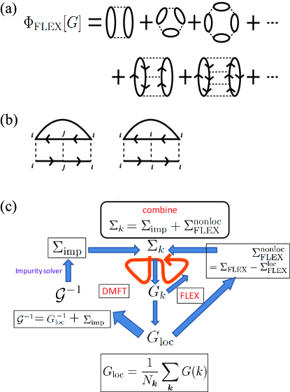
Figure 1: (Color online) (a) The Luttinger-Ward functional for FLEX. particle-particle (b) An example of a diagram contained in $\Sigma_{{\rm FLEX},ii}^{\rm nonloc}$ (left, with $i\neq j$) and omitted (right). (c) Self-consistent double loops in the FLEX+DMFT formalism. The algorithm flow for the loops is indicated by the red arrow.

The present scheme may be viewed as a new diagrammatic extension of the DMFT that incorporates vertex corrections into the (local part of) FLEX scheme. FLEX itself, being a perturbative method, is considered to become exact in the weak-coupling limit, while DMFT becomes exact in the atomic limit. Since FLEX+DMFT formalism here incorporates the functionals that dominate in either limit, it is expected to describe spin fluctuation effects and Mott’s physics simultaneously.

III Application to the 2D Hubbard model

Let us apply the FLEX+DMFT method to the repulsive Hubbard model on the square lattice, with a Hamiltonian,

$${\cal H}=\sum_{{\boldsymbol{k}},\sigma}\epsilon({\boldsymbol{k}})c_{{\boldsymbol{k}},\sigma}^{{\dagger}}c_{{\boldsymbol{k}},\sigma}+U\sum_{i}n_{i,\uparrow}n_{i,\downarrow}.$$ (4)

Here $c_{{\boldsymbol{k}},\sigma}^{{\dagger}}$ creates an electron in a Bloch state with wave-vector ${\mbox{\boldmath$k$}}=(k_{x},k_{y})$ and spin $\sigma$, $U$ is the on-site repulsion, and $n_{i,\sigma}=c_{i,\sigma}^{{\dagger}}c_{i,\sigma}$ is the number operator. The two-dimensional band dispersion is given as

$$\epsilon({\boldsymbol{k}}) =-2t({\rm cos}k_{x}+{\rm cos}k_{y})$$

$$\quad-4t^{\prime}{\rm cos}k_{x}{\rm cos}k_{y}-2t^{\prime\prime}({\rm cos}2k_{x}+{\rm cos}2k_{y})-\mu,$$ (5)

where $t,t^{\prime},$ and $t^{\prime\prime}$ represent the nearest-neighbor, second-neighbor, and third-neighbor hoppings, respectively, while $\mu$ is the chemical potential. We shall compare the case with the nearest-neighbor hopping only ($t^{\prime}/t=t^{\prime\prime}/t=0$) with the case of $t^{\prime}/t=-0.20$, $t^{\prime\prime}/t=0.16$, which are the values estimated for a typical hole-doped, single-layered cuprate, HgBa₂CuO_4+δ with $T_{c}\simeq 90$K, with first-principles methods.nishiguchi_prb ; sakakibara Hereafter we take $|t|$ as the unit of energy.

In the single-band Hubbard model, the FLEX self-energy is computed as

$$\Sigma_{\rm FLEX}(k)=\frac{1}{N_{\bm{k}}\beta}\sum_{k^{\prime}}\Bigl{[}\frac{3}{2}U^{2}\frac{\chi_{0}(k-k^{\prime})}{1-U\chi_{0}(k-k^{\prime})}$$

$$+\frac{1}{2}U^{2}\frac{\chi_{0}(k-k^{\prime})}{1+U\chi_{0}(k-k^{\prime})}-U^{2}\chi_{0}(k-k^{\prime})\Bigr{]}G(k^{\prime}),$$ (6)

where $\beta$ is the inverse temperature, $k=(\omega_{n},{\boldsymbol{k}})$ with $\omega_{n}$ the fermionic Matsubara frequency, $G(k)$ is the Green’s function, and

$$\chi_{0}(q)=-\frac{1}{N_{\bm{k}}\beta}\sum_{k}G(k+q)G(k)$$ (7)

is the irreducible susceptibility. We can calculate $\Sigma^{\rm loc}_{\rm FLEX}$ by replacing $G$ with $G_{\rm loc}$ in Eqs. (6) and (7).

To obtain $\Sigma_{\rm imp}$ in the DMFT procedure, we have to solve the impurity problem in DMFT. Among various impurity solvers, here we adopt the modified iterative perturbation theory (modified IPT), where the original IPT is modified for systems without particle-hole symmetry.mIPT The method is not computationally demanding, which facilitates a scanning over a wide parameter region to obtain the phase diagram, and also enables us to approach a region with large antiferromagnetic fluctuations where FLEX convergence critically slows down. We have confirmed for various values of parameters that the continuous-time quantum Monte Carlo impurity solver CTQMC ; CTQMC-review implemented with the ALPS libraryALPS1 ; ALPS2 gives similar values for the eigenvalue of Eliashberg’s equation even away from the half-filling.

When Green’s function is obtained, we plug it into the linearized Eliashberg equation,

$$\lambda\Delta(k)=-\frac{1}{N_{\bm{k}}\beta}\sum_{k^{\prime}}V_{\rm eff}(k-k^{\prime})G(k^{\prime})G(-k^{\prime})\Delta(k^{\prime}).$$ (8)

Here $\Delta(k)$ is the anomalous self-energy, which is the gap function up to the renormalization factor, and

$$V_{\rm eff}(k)=U+\frac{3}{2}U^{2}\frac{\chi_{0}(k)}{1-U\chi_{0}(k)}-\frac{1}{2}U^{2}\frac{\chi_{0}(k)}{1+U\chi_{0}(k)}$$ (9)

is the effective pairing interaction (Fig. 2), where $\lambda$ is the eigenvalue for Eliashberg’s equation, with superconducting transition identified as the temperature at which $\lambda=1$.

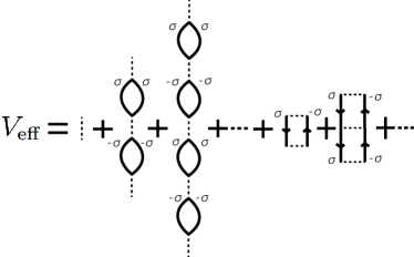
Figure 2: Effective pairing interaction in the FLEX.

At this point we should mention about the consistency of the approximate functional form $\Phi_{\rm FLEX+DMFT}$ and the linearized Eliashberg equation, Eq. (8). The Luttinger-Ward functional can be extended to incorporate the anomalous part, and the extended functional $\Phi[G,F^{{\dagger}},F]$ is related to the anomalous self-energy through $\Delta=\delta\Phi/\delta F^{{\dagger}}$, where $F^{{\dagger}}$ is the anomalous Green’s function, for which we should consider the local correction to the anomalous self-energy $\Delta$ as $\Delta_{\rm FLEX+DMFT}=\Delta_{\rm FLEX}+\Delta_{\rm loc}$ as in Eq. (2) for the normal self-energy. Now, our interest here is the anisotropic, $d$-wave pairing instability in the repulsive model, for which we can ignore the local correction to the anomalous self-energy $\Delta_{\rm loc}$ which does not depend on momentum. The remaining term $\Delta_{\rm FLEX}=\delta\Phi_{\rm FLEX}[G,F^{{\dagger}},F]/\delta F^{{\dagger}}$ is the same as the right-hand side of the linearized Eliashberg equation (8) if we linearize the anomalous part.FLEX_functional Then our formalism treats the normal and anomalous self-energies consistently, as functional derivatives of the same Luttinger-Ward functional $\Phi_{\rm FLEX+DMFT}$. This is an advantage of using the Luttinger-Ward functional formalism in constructing a new scheme.

IV Results

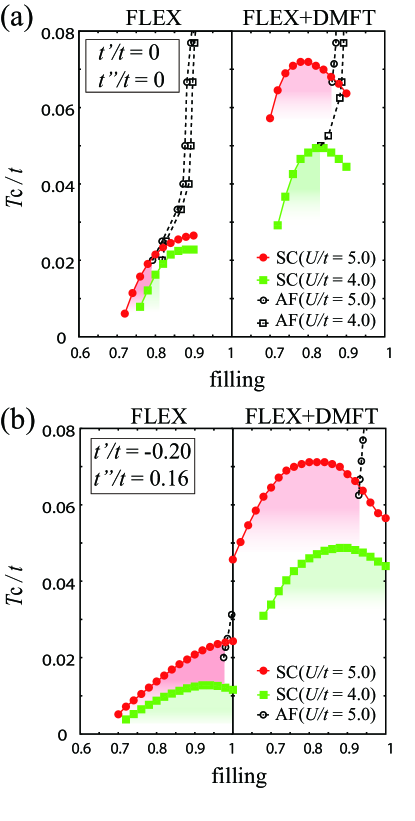
Figure 3: (Color online) Phase diagram against the band filling $n$ and the temperature $T/t$ in the FLEX+DMFT (right panels) as compared with FLEX (left). Here we take $U/t=4.0,5.0$ and (a) $t^{\prime}/t=t^{\prime\prime}/t=0$, or (b) $t^{\prime}/t=-0.20,t^{\prime\prime}/t=0.16$. We also plot the AF phase boundaries (dotted lines) in the normal region, while color shading highlights the superconducting region with $T_{c}>T_{\rm AF}$ at each filling.

We show the superconducting phase diagram of the two-dimensional Hubbard model obtained in the FLEX+DMFT in Fig. 3, right panels, where the FLEX result is also displayed in the left panels for comparison. We can immediately see that $T_{c}$ exhibits a dome structure in the FLEX+DMFT. This sharply contrasts with the FLEX result, where $T_{c}$ has been known to almost monotonically increase toward half-filling with some rounding off.review_yanase The presence of the $T_{c}$ dome in the FLEX+DMFT and its absence in the FLEX are seen for both the simple square lattice with $t^{\prime}=t^{\prime\prime}=0$ [Fig. 3(a)] and the case of $t^{\prime}=-0.20,t^{\prime\prime}=0.16$ [Fig. 3(b)].

For the simple square lattice ($t^{\prime}=t^{\prime\prime}=0$), we cannot approach a region very close to half-filling because the antiferromagnetic (AF) fluctuations prevent the FLEX self-consistency loop from converging. For the same reason, it is difficult to attain convergence for systems with larger $U$. As a measure of the AF order, we evaluated the AF phase boundaries (dashed lines in Fig. 3) determined from ${\rm max}_{k}[U\chi_{0}(k)](=0.99$ here),AF which is usually adopted in FLEX-type schemes to take account of the effect of the quasi-two-dimensional nature (e.g., in three-dimensional layered systems), although FLEX-type approaches are known to obey the Mermin-Wagner theorem that forbids finite-temperature AF phase transitions in an isolated two-dimensional system. The estimated AF transition temperature $T_{\rm AF}$ becomes higher than the superconducting $T_{c}$ as one approaches half-filling as shown in Fig. 3, where the color shaded region indicates the superconducting phase with $T_{c}>T_{\rm AF}$ (i.e., superconductivity dominating antiferromagnetism). The result suggests that a part of the $T_{c}$ dome is taken over by the AF phase in the case of $t^{\prime}=t^{\prime\prime}=0$ [Fig. 3(a), right] and $t^{\prime}=-0.20,t^{\prime\prime}=0.16,U=5$ [Fig. 3(b), right]. For a smaller $U=4$, by contrast, we have an almost full $T_{c}$ dome with $T_{c}>T_{\rm AF}$ for $t^{\prime}=-0.20,t^{\prime\prime}=0.16$ [Fig. 3(b), right]. These are a key result in the present work.

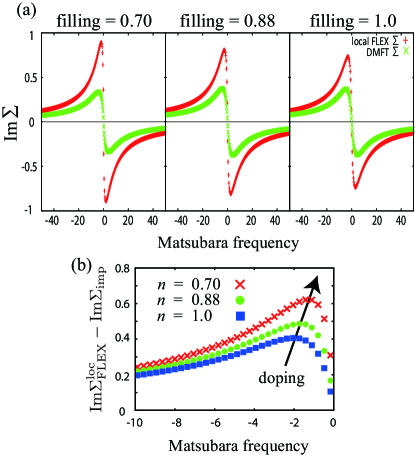
Figure 4: (Color online) (a) Comparison between the FLEX local self-energy ${\rm Im}\Sigma^{\rm loc}_{\rm FLEX}$ (red plus signs) and the DMFT self-energy ${\rm Im}\Sigma_{\rm imp}$ (green crosses) for the filling $n=0.70$ (underdoped; left panel), $0.88$ (optimally doped; center), and $1.0$ (half-filled; right). (b) The difference, Im$\Sigma^{\rm loc}_{\rm FLEX}-$Im$\Sigma_{\rm imp}$, for $n=0.70$ (red crosses), $0.88$ (green circles), and $1.0$ (blue squares). Here we take $U/t=4.0$, $\beta=20$, $t^{\prime}/t=-0.20$, and $t^{\prime\prime}/t=0.16$.

Now let us identify the physical origin of the appearance of the $T_{c}$ dome in the FLEX+DMFT. In FLEX+DMFT, the self-energy is obtained from the FLEX and DMFT self-energies as $\Sigma_{\rm FLEX+DMFT}=\Sigma_{\rm FLEX}-(\Sigma_{\rm FLEX}^{\rm loc}-\Sigma_{\rm imp})$ [Eqs. (2) and (3)], i.e., a part of the local self-energy is replaced from that in FLEX with that in DMFT. Thus the quantity $\Sigma_{\rm FLEX}^{\rm loc}-\Sigma_{\rm imp}$ represents the difference in the self-energy effect between FLEX and FLEX+DMFT. We can actually take a look at $\Sigma^{\rm loc}_{\rm FLEX}$ and $\Sigma_{\rm imp}$, with fillings $n=0.7$ (underdoped), $0.88$ (optimally doped), and $1.0$ (half-filled) in Fig. 4 [the parameters are taken to be $U=4.0,\beta=20,t^{\prime}=-0.20,t^{\prime\prime}=0.16$, which corresponds to Fig. 3(b), right panel]. We first notice that the magnitude of the DMFT self-energy $\Sigma_{\rm imp}$ is smaller than that of FLEX $\Sigma_{\rm FLEX}^{\rm loc}$, which means that the overestimation of the self-energy generally known to exist in FLEX is remedied in FLEX+DMFT by the DMFT (local) vertex corrections. More importantly, we can see that the difference, ${\rm Im}\Sigma^{\rm loc}_{\rm FLEX}-{\rm Im}\Sigma_{\rm imp}$ [Fig. 4(b)], has a clear filling dependence, and it increases with doping. Since $\Sigma_{\rm FLEX+DMFT}=\Sigma_{\rm FLEX}-(\Sigma_{\rm FLEX}^{\rm loc}-\Sigma_{\rm imp})$, the result indicates that the reduction of the FLEX+DMFT self-energy due to DMFT correction is reduced as one approaches half-filling. Thus $T_{c}$ tends to be suppressed near half-filling as compared to that of FLEX because of the filling-dependent self-energy reduction in FLEX+DMFT. On the other hand, the pairing interaction itself arising from spin fluctuations becomes stronger toward half-filling due to better band nesting, as reflected in the FLEX result [Fig. 3, left panels] with $T_{c}$ almost monotonically increasing toward half-filling. Therefore, the FLEX+DMFT contains two factors with opposite filling dependencies, and we conclude that the $T_{c}$ dome in FLEX+DMFT arises from the combined effect of the nesting and filling-dependent self-energy reduction.

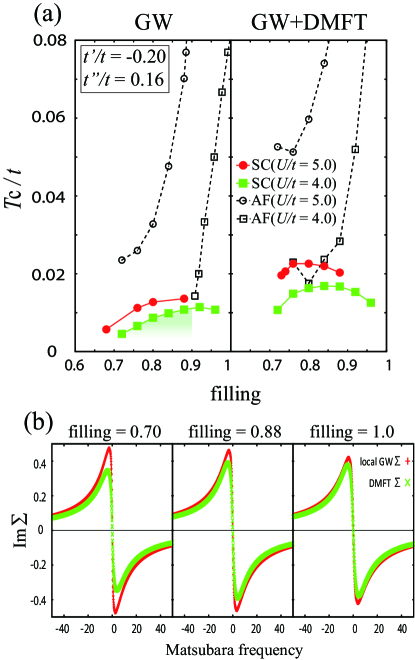
Figure 5: (Color online) (a) Phase diagram against temperature $T/t$ and band filling $n$ in GW+DMFT approximation (right) as compared with that in GW approximation (left) for $U/t=4.0$ (green squares) or $U/t=5.0$ (red circles). (b) Comparison between the GW local self-energy ${\rm Im}\Sigma^{\rm loc}_{\rm GW}$ (red plus signs) and the DMFT self-energy ${\rm Im}\Sigma_{\rm imp}$ (green crosses) for the filling $n=0.70$ (left panel), $0.88$ (center), and $1.0$ (right) with $U/t=4.0$ and $\beta=50$. Here we take $t^{\prime}/t=-0.20$, $t^{\prime\prime}/t=0.16$. We also plot antiferromagnetic (AF) phase boundaries (dotted lines) in the normal region, while color shading highlights the dome in the region where $T_{c}$ is above the AF boundary.

In the FLEX+DMFT scheme, the self-energy reduction from DMFT takes place only in the local part, while the nonlocal self-energy is still considered to be overestimated, especially for ladder diagrams.MBPT+DMFT To examine this effect, we compare the present method with GW+DMFT, where only the bubble diagrams are considered for the self-energy and the pairing interaction (whereas both bubbles and ladders are included in FLEX and FLEX+DMFT). We show the GW+DMFT phase diagram, along with the GW result for comparison, in Fig. 5 for $t^{\prime}=-0.20$ and $t^{\prime\prime}=0.16$. We can see that, although the $T_{c}$ dome structure remains in the GW+DMFT result, $T_{c}$ is much reduced from the result of FLEX+DMFT. On the other hand, the AF transition temperature is much higher in GW+DMFT than that of FLEX+DMFT. This makes the region in the dome where $T_{c}>T_{\rm AF}$ [highlighted with color shadings in Fig. 5(a)] very narrow in GW+DMFT. In fact, for $t^{\prime}=t^{\prime\prime}=0$ the AF instability becomes so strong that we cannot even obtain superconducting phase boundaries for the whole region of the fillings considered.

In Fig. 5(b), we display the GW local self-energy ${\rm Im}\Sigma^{\rm loc}_{\rm GW}$ as compared with the DMFT self-energy ${\rm Im}\Sigma_{\rm imp}$ for the filling $n=0.70,0.88,1.0$ with $U=4.0$ and $\beta=50$. We can see that the filling dependence is similar to those in the FLEX+DMFT in that the difference between the two self-energies increases with the doping. Hence we can conclude that the existence of the $T_{c}$ dome is not an artifact in FLEX+DMFT, but is robust in both FLEX+DMFT and GW+DMFT arising due to the same local vertex correction effect. The overestimation of nonlocal self-energy thus does not affect the existence of the $T_{c}$ dome itself.

The reason that the magnitude of $T_{c}$ is much smaller in GW+DMFT than in FLEX+DMFT is because ladder diagrams describing spin fluctuations are not taken into account in GW+DMFT. In this sense, GW+DMFT is closer to the mean-field theory than FLEX+DMFT, which is also reflected in the higher AF transition temperature in GW+DMFT. Concomitantly, the pairing interaction mediated by spin fluctuations is reduced, which acts to reduce the superconducting $T_{c}$ in GW+DMFT rather than in FLEX+DMFT. The fact that $T_{c}$ is always estimated below the Néel temperature in GW+DMFT suggests that GW+DMFT underestimates the spin fluctuation effect, and is not enough to describe the $d$-wave superconductivity mediated by spin fluctuations. Since the overestimated nonlocal self-energy in FLEX+DMFT is remedied in GW+DMFT, the accurate estimation of the spin-fluctuation effect is expected to lie between GW+DMFT and FLEX+DMFT.

To see the strength of local correlation, we measure the double occupancy,

$$\left<n_{\uparrow}n_{\downarrow}\right>=\frac{1}{U}{\rm Tr}(\Sigma G).$$ (10)

We can see in Fig. 6 that the double occupancy becomes negative in the overdoped regime in FLEX, while this unphysical behavior is improved in FLEX+DMFT. We can regard this as another of the self-energy reduction effects: FLEX overestimates the correlation effect, while this is corrected by combining it with the DMFT. A similar tendency is observed between GW and GW+DMFT, but the difference in the double occupancy is smaller. This should be because the self-energy reduction effect is smaller [see Figs. 4(a) and 5(b)].

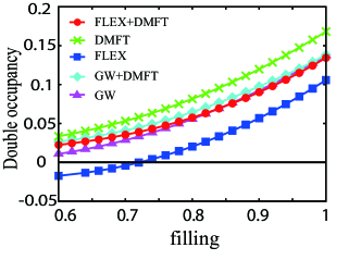
Figure 6: (Color online) Double occupancy against band filling $n$ in the FLEX+DMFT (red circles), DMFT (green crosses), FLEX (blue squares), GW+DMFT (light blue diamonds), and GW (purple triangles). Here we take $U/t=4.0$, $\beta=20$, $t^{\prime}/t=-0.20$, and $t^{\prime\prime}/t=0.16$.

Let us finally examine the spectral function, which is calculated via analytical continuation with the Padé approximation. The results for FLEX+DMFT, FLEX, GW, GW+DMFT, and DMFT at various fillings are shown in Fig. 7. We can see that the filling dependence is similar among FLEX, GW, and DMFT in that we have a single peak that slightly shifts and broadens as we approach the half-filling. By contrast, in the method that combines DMFT with either FLEX or GW, the spectral function acquires a stronger filling dependence, where a marked double peak is observed at half-filling. Similar double-peak structures have been reported in the dual-fermion methodDF2009_2 as an antiferromagnetic pseudogap, where the appearance of the double peak is consistent with the QMC result. Thus we can see that the interplay of the local and nonlocal long-range correlation effects in FLEX+DMFT and GW+DMFT gives the double peak, which is considered to be a precursor of the Hubbard bands with two peaks separated by about $U$, while the system is metallic.

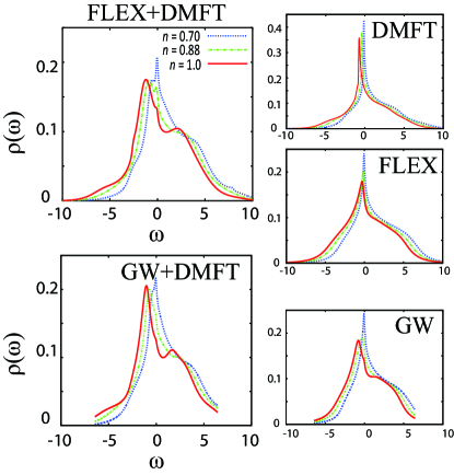
Figure 7: (Color online) Spectral functions at filling $n=0.70$ (underdoped; dotted lines), 0.88 (optimally doped; green), 1.0 (half-filling; red) in the FLEX+DMFT (top left) and GW+DMFT (bottom left) are compared with those in DMFT (top right), FLEX (middle right), and GW (bottom right). Here we take $U/t=4.0$, $\beta=20$, $t^{\prime}/t=-0.20$, and $t^{\prime\prime}/t=0.16$.

If we look more closely at the momentum-resolved spectral function $A({\boldsymbol{k}},\omega)$, we observe that there is a region in $k$ space near the Fermi energy where the spectral weight becomes slightly negative. This might not be specific to the present method, since many extensions of DMFT do not guarantee positive-definite spectral weights.DF2009 ; one-particle-irr Since the magnitude of the negative part is negligibly small ($<1\%$) in the present case and this tends to occur in the overdoped regime, this does not affect the phase diagram and the density of states [Figs. 3 and 7] in the underdoped regime.

V Summary and discussions

We have employed the FLEX+DMFT approach in terms of a new Luttinger-Ward functional to study the superconductivity in correlated electron systems. This scheme is a diagrammatic extension of the DMFT, so that it can describe the $d$-wave superconductivity arising from $k$-dependent pairing interaction. The scheme, being formulated in terms of the Luttinger-Ward functional, also has a virtue of the normal and anomalous self-energies treated on an equal footing. We have applied the FLEX+DMFT to the repulsive Hubbard model on the square lattice. We have found that FLEX+DMFT describes a $T_{c}$ dome structure, whose physical origin is traced back to a combination of opposite effects: The self-energy effect introduced in the FLEX+DMFT suppresses the superconductivity more strongly toward the half-filling due to the local-correlation effect, while spin fluctuations become stronger toward the half-filling due to band nesting. We also compare the FLEX+DMFT result with the GW+DMFT result, which reproduces the dome structure. This indicates that the dome is not an artifact of the overestimated nonlocal self-energy in FLEX+DMFT.

Another observation is that there is a Pomeranchuk instability into electronic states with broken tetragonal symmetry in the case of $t^{\prime}=-0.20,t^{\prime\prime}=0.16$ in both FLEX+DMFT and GW+DMFT. In this case, solutions with the four-fold rotationally symmetric Fermi surface become unstable, where we end up with a solution that breaks this symmetry when we start the calculation from an asymmetric initial input. While this instability is interesting in its own right, we have concentrated on the symmetric case in this study, and leave the analysis of the Pomeranchuk instability to another publication.

In order to improve the scheme to suppress the overestimation of the nonlocal FLEX self-energy, we should consider the screening effect in the FLEX self-energy. For example, the two-particle self-consistent method TPSC takes account of vertex correction effects by considering the sum rule for the susceptibility, while a similar technique is also used to reduce the overestimated spin fluctuations and their effect on the self-energy in D$\Gamma$A.DgammaA-lambda We expect these techniques bring some improvement to the present theory.

VI Acknowledgement

The authors wish to thank K. Nishiguchi for providing a FLEX coding and fruitful discussions, and J. Otsuki and H. Hafermann for useful discussions. The present work was supported by a Grant-in-Aid for Scientific Research (Grant No. 26247057) from MEXT, M.K. was supported by the advanced leading graduate course for photon science (ALPS), and N.T. was supported by a Grant-in-Aid for Scientific Research (Grant No. 25800192) from JSPS.

References

- (1) J. G. Bednorz and K. A. Müller, Z. Phys. B 64, 189 (1986).
- (2) D. J. Scalapino, Rev. Mod. Phys. 84, 1383 (2012).
- (3) D. J. Scalapino, E. Loh, Jr., and J. E. Hirsch, Phys. Rev. B 35, 6694 (1987).
- (4) N. F. Mott and R. Peierls, Proc. Phys. Soc. 49, 72 (1937).
- (5) J. E. Hirsch, Phys. Rev. B 31, 4403 (1985).
- (6) N. E. Bickers, D. J. Scalapino, and S. R. White, Phys. Rev. Lett. 62,8 (1989).
- (7) W. Metzner and D. Vollhardt, Phys. Rev. Lett. 62,324 (1989).
- (8) A. Georges and G. Kotliar, Phys. Rev. B 45, 6479 (1992).
- (9) A. Georges, G. Kotliar, W. Krauth, and M. J. Rozenberg, Rev. Mod. Phys. 68, 13 (1996).
- (10) M. H. Hettler, A. N. Tahvildar-Zadeh, M. Jarrell, T. Pruschke, and H. R. Krishnamurthy, Phys. Rev. B 58, R7475(R) (1998).
- (11) G. Kotliar, S. Y. Savrasov, G. Palsson, and G. Biroli, Phys. Rev. Lett. 87,186401 (2001).
- (12) S. Sakai, Y. Motome, and M. Imada, Phys. Rev. Lett. 102,056404 (2009).
- (13) E. Gull, O. Parcollet, and A. J. Millis Phys. Rev. Lett. 110,216405 (2013).
- (14) P. Sun and G. Kotliar, Phys. Rev. B 66, 085120 (2002).
- (15) S. Biermann, F. Aryasetiawan, and A. Georges, Phys. Rev. Lett. 90,086402 (2003).
- (16) A. Toschi, A. A. Katanin, and K. Held, Phys. Rev. B 75, 045118 (2007).
- (17) A. A. Katanin, A. Toschi, and K. Held, Phys. Rev. B 80, 075104 (2009).
- (18) A. N. Rubtsov, M. I. Katsnelson, and A. I. Lichtenstein, Phys. Rev. B 77, 033101 (2008).
- (19) S. Brener, H. Hafermann, A. N. Rubtsov, M. I. Katsnelson, and A. I. Lichtenstein, Phys. Rev. B 77, 195105 (2008).
- (20) A. N. Rubtsov, M. I. Katsnelson, A. I. Lichtenstein, and A. Georges, Phys. Rev. B 79, 045133 (2009).
- (21) H. Hafermann, G. Li, A. N. Rubtsov, M. I. Katsnelson, A. I. Lichtenstein, and H. Monien, Phys. Rev. Lett. 102,206401 (2009).
- (22) G. Rohringer, A. Toschi, H. Hafermann, K. Held, V. I. Anisimov, and A. A. Katanin, Phys. Rev. B 88, 115112 (2013).
- (23) C. Taranto, S. Andergassen, J. Bauer, K. Held, A. Katanin, W. Metzner, G. Rohringer, and A. Toschi, Phys. Rev. Lett. 112,196402 (2014).
- (24) J. Gukelberger, L. Huang, and P. Werner, Phys. Rev. B 91, 235114 (2015).
- (25) We should note that FLEX+DMFT is totally different from the method called DMFT(FLEX) in K. Aryanpour, M. H. Hettler, and M. Jarrell, Phys. Rev. B 67, 085101 (2003), where FLEX is used as an impurity solver to treat large clusters within dynamical cluster approximation.
- (26) J. Otsuki, H. Hafermann, and A. I. Lichtenstein, Phys. Rev. B 90, 235132 (2014).
- (27) J. M. Luttinger and J. C. Ward, Phys. Rev. 118,1417 (1960).
- (28) G. Baym and L. P. Kadanoff, Phys. Rev. 124,287 (1962).
- (29) G. Baym, Phys. Rev. 127,1391 (1962).
- (30) While we do not take account of the particle-particle ladder diagrams for the FLEX self-energy in this paper, we have checked that the result remains almost the same when we consider the diagrams, especially when we combine those with DMFT in the present FLEX+DMFT.
- (31) K. Nishiguchi, K. Kuroki, R. Arita, T. Oka, and H. Aoki, Phys. Rev. B 88, 014509 (2013); K. Nishiguchi, Ph.D. thesis, University of Tokyo, 2013.
- (32) Similar values are also obtained in H. Sakakibara, H. Usui, K. Kuroki, R. Arita, and H. Aoki, Phys. Rev. Lett. 105,057003 (2010).
- (33) H. Kajueter and G. Kotliar, Phys. Rev. Lett. 77,131 (1996).
- (34) A. N. Rubtsov, V. V. Savkin, and A. I. Lichtenstein, Phys. Rev. B 72, 035122 (2005).
- (35) E. Gull, A. J. Millis, A. I. Lichtenstein, A. N. Rubtsov, M. Troyer, and P. Werner, Rev. Mod. Phys. 83, 349 (2011).
- (36) B. Bauer, et al., J. Stat. Mech. P05001 (2011).
- (37) A. F. Albuquerque, et al., J. Magn. Magn. Mater. 310,1187 (2007).
- (38) Y. Yanase and M. Ogata, J. Phys. Soc. Jpn. 74, 1534 (2005).
- (39) Y. Yanase, T. Jujo, T. Nomura, H. Ikeda, T. Hotta, and K. Yamada, Phys. Rep. 387, 1 (2003).
- (40) The present estimate of the AF susceptibility is only on the mean-field level, while for a more precise treatment one should solve the Bethe-Salpeter equation by using as the interaction kernel, which will somewhat reduce for (quasi-)two dimensional systems.
- (41) Y. M. Vilk and A.-M. S. Tremblay, J. Phys. I France 7, 1309 (1997).