Approximation solution of two-dimensional linear stochastic Volterra integral equation by applying the Haar wavelet

Mathematical subject classification: 65C30, 65C20, 60H20, 60H35, 68U20.
Keywords: Haar wavelet; Two-dimensional stochastic Volterra integral equation; Brownian motion process; Ito integral.

1. Introduction

As we know, two dimensional ordinary integral equations provide an important tool for modeling a numerous problems in engineering and science $[6,7]$. The second kind of two-dimensional integral equations may arise from some problems of nonhomogeneous elasticity and electrostatics $[8]$.

Dobner presented an equivalent formulation of the Dorboux problem as a two-dimensional Volterra integral equation $[9]$. We can also see this kind of equations in contact problems for bodies with complex properties $[10,11]$, and in the theory of radio wave propagation $[12]$, and in the theory of the elastic problem of axial translation of a rigid elliptical disc-inclusion $[13]$, and various physical, mechanical and biological problems. Some numerical schemes have been inspected for resolvent of two-dimensional ordinary integral equations by several probers. Computational complexity of mathematical operations is the most important obstacle for solving ordinary integral equations in higher dimensionas.

The Nystrom method $[14]$, collocation method $[15,16,17]$, Gauss product quadrature rule method $[18]$, Galerkin method $[19]$, using triangular fuctions $[20,21]$, Legender polynomial method $[22]$, differential transform method $[23]$, meshless method $[24]$, Bernstein polynomials method $[25]$ and Haar wavelet method $[26]$. This paper is first focused on proposing a generic framework for numerical solution of two-dimensional ordinary linear Volterra integral equations of second kind. The use of the Haar wavelet for the numerical solution of linear integral equations has previously been discussed in $[1]$ and references therein. The paper $[1]$ should be considered as a logical continuation of the papers $[2-4]$. In $[2]$ a new numerical method based on Haar wavelet is introduced for solution of nonlinear one-dimensional Fredholm and Volterra integral equations. In $[3]$ the Haar wavelet method $[2]$ is extended to numerical solution of integro-differential equation. In $[4]$ the Haar wavelet method $[2,3]$ is improved in terms of efficiency by introducing one-dimentional Haar wavelet approximation of the kernel function. The method $[1]$ is fundamentally different from the other numerical methods based on Haar wavelet for the numerical solution of integral equations as it approximates kernel function using Haar wavelet.

The general hyperbolic differential equation is defined as $[9]$

(1.1) $$u_{xy}=r(x,y,u,u_{x},u_{y})\ \ ,\ \ {(x,y)\in B}\subseteq{\mathbb{R}^{2}}$$

$$u_{1\hat{B}}=h(x,y)\ \ \ \ ,\ \ \ \ \hat{B}\subseteq\partial B,$$

where the domain $B$ and the subset $\hat{B}$ of the border $\partial B$ are chosen according to the different initial value problems. It’s easy to show that the integral form of $(1.1)$ is given by two-dimentional Volterra integral equation

$$g(x,y)=f(x,y)+\int_{0}^{y}\int_{0}^{x}K_{1}(x,y,s,t)g(s,t)dsdt.$$

Similarly, if we import statistical noise in to $(1.1)$, we can obtain two-dimensional linear stochastic Volterra integral equation of the second kind, i.e.

(1.2) $$g(x,y)=f(x,y)+\int_{0}^{y}\int_{0}^{x}K_{1}(x,y,s,t)g(s,t)dsdt$$

$$\ \ \ \ \ \ \ \ \ \ \ \ \ \ \ \ \ \ \ \ \ \ \ \ \ \ \ \ \ \ \ +\int_{0}^{y}\int_{0}^{x}K_{2}(x,y,s,t)g(s,t)dB(s)dB(t)$$

$$\ \ \ \ \ \ \ \ \ \ \ \ \ \ \ \ \ \ \ \ \ \ \ \ \ \ \ \ \ \ \ \ \ \ \ \ \ \ \ \ \ \ \ \ \ \ \ \ \ \ \ \ \ \ \ \ \ \ \ \ \ \ (x,y)\in[0,1]\times[0,1]\ \ \ ,\ \ \ {s}\leqslant{x<t}\leqslant{y.}$$

where the kernels $K_{1}(x,y,s,t)$ and $K_{2}(x,y,s,t)$ in $(1,2)$ are known functions and $f(x,y)$ is also a known function whereas $g(x,y)$ is unknown function and is called the solution of two-dimensional stochastic integral equation. The condition $s\leqslant x<t\leqslant y$ is necessary for adaptability to the filtration $\{F_{t};0\leq t\leq 1\}$ where $F_{t}=\sigma\{B(s);0\leq s\leq 1\}$.

Lemma 1.Put $\phi(t,s)=K(x,y,s,t)g(s,t)$. Let $\phi$ be a function in ${\textit{L}}^{2}([0,1]^{2})$. Then there exists a sequence ${\phi_{n}}$ of off-diagonal step functions such that

$$\lim_{n\rightarrow\infty}\int_{a}^{b}\int_{a}^{b}\mid\phi(t,s)-\phi_{n}(t,s)\mid^{2}dtds=0.$$

Definition 1. Let $\phi\in\textit{L}^{2}([0,1]^{2})$. Then the double Wiener-It$\hat{\textbullet}$o integral of ${\phi}$ is defined as

$$\int_{a}^{b}\int_{a}^{b}\phi(t,s)dB(t)dB(s)=\lim_{n\rightarrow\infty}\int_{a}^{b}\int_{a}^{b}\phi_{n}(t,s)dB(t)dB(s)\ \ \ \ \ \ in\ \ \ \textit{L}^{2}(\Omega).$$

2. Haar Wavelets

A wavelet family $(\psi_{j},_{i}\left(y\right))_{j\in{N},i\in{Z}}$ is an orthonormal subfamily of the Hilbert space $L^{2}(R)$ with the property that all function in the wavelet family are generated from a fixed function $\psi$ called mother wavelet through dilations and translations.The wavelet family satisfies the following relation

$$\psi_{j},_{i}\left(y\right)=2^{j/2}\psi\left(2^{j}y-i\right).$$

For Haar wavelet family on the interval $[0,1)$ we have:

$$h_{1}(y)=\left\{\begin{array}[]{cc}1,&for$y$\in[0,1)\\ 0,&otherwise,\end{array}\right.$$

$$h_{i}(y)=\left\{\begin{array}[]{cc}1&for$y$\in[\alpha,\beta)\\ -1,&for$y$\in[\beta,\gamma)\\ 0,&\ \ \ \ \ \ otherwise,\ \ \ \ \ i=2,3,...,\end{array}\right.$$

$$\alpha=\frac{n}{m},\ \ \ \ \beta=\frac{(n+0.5)}{m},\ \ \ \ \gamma=\frac{(n+1)}{m};$$

$$\ m=2^{\ell},\ \ \ \ \ \ \ell=0,1,...,\ \ \ \ \ \ n=0,1,...,m-1.$$

The integer $\ell$ indicats the level of the wavelet and $n$ is the translation parameter. Any square integrable function $f(y)$ defined on $[0,1)$ can be expressed as follows:

$$f(y)=\sum_{i=1}^{\infty}a_{i}h_{i}(y),$$

where $a_{i}$ are real constants.
For approximation aim we consider a maximum value $L$ of the integer $\ell,$ level of the Haar wavelet in the above definition. The integer $L$ is then called maximum level of resolution. We also define integer $M=2^{L}$. Hence for any square integrable function $f(y)$ we have a finite sum of Haar wavelets as follows:

$$f(y)\thickapprox\sum_{i=1}^{2M}a_{i}h_{i}(y).$$

The following notation is introduced $[1]$:

(2.1) $$p_{i,1}(y)=\int_{0}^{y}h_{i}(u)du,$$

where by the definition of Haar wavelet equation $(2.1)$ reduce to

$$p_{i,1}(y)=\left\{\begin{array}[]{cc}y-\alpha,&\ \ \ \ \ \ \ for$ y $\in[\alpha,\beta)\\ \gamma-y,&\ \ \ \ \ \ \ for$ y $\in[\beta,\gamma)\\ 0,&\ \ \ elsewhere.\end{array}\right.$$

We can also the following stochastic notation introduce

(2.2) $$q_{i,1}(y)=\int_{0}^{y}h_{i}(u)dB(u),$$

where equation $(2.2)$ can be evaluated similarly by the definition of Haar wavelet and is given as follow:

$$q_{i,1}(y)=\left\{\begin{array}[]{cc}B(y)-B(\alpha),&\ \ \ \ \ \ for$ y $\in[\alpha,\beta)\\ 2B(\beta)-B(\alpha)-B(y),&\ \ \ \ \ \ \ for$ y $\in[\beta,\gamma)\\ 0,&\ \ \ elsewhere.\end{array}\right.$$

3. Numerical method

In this section, proposed numerical method $[1]$ will be discussed for two-dimensional linear stochastic Volterra integral equation of the second kind. In the first subsection, we state some results for efficient evalution of two-dimensional Haar wavelet approximations. In the second subsection, we apply these results for finding numerical solutions equation $(1.1)$.
For Haar wavelet approximation of a function $f(x,y)$ of two real variables $x$ and $y$, we assume that the domain $0\leq x,y\leq 1$ is divided into a grid of size $2M\times 2N$ using the following collocation points

(3.1) $$x_{m}=\frac{m-0.5}{2M},m=1,2,...,2M,$$

(3.2) $$y_{n}=\frac{n-0.5}{2N},n=1,2,...,2N.$$

3.1     Two-dimensional Haar wavelet system

A real-valued function $G(x,y)$ of two real variables $x$ and $y$ can be approximated using two-dimensional Haar wavelets basis as $[1,27]$:

(3.3) $$G(x,y)\thickapprox\sum_{p=1}^{2M}\sum_{q=1}^{2N}b_{p,q}h_{p}(x)h_{q}(y).$$

In order to calculate the unknown coefficients $b_{i,j}$’s, the collocation points defined in Eqs. $(3.1)$ and $(3.2)$ are substituted in Eq. $(3.3)$.Hence, we obtain the following $2M\times 2N$ linear system with unknowns $b_{i,j}$’s:

(3.4) $$G(x_{m},y_{n})=\sum_{p=1}^{2M}\sum_{q=1}^{2N}b_{p,q}h_{p}(x_{m})h_{q}(y_{n}),m=1,2,...,2M,\ \ \ n=1,2,...,2N.$$

The solution of system $(3.4)$ can be calculated from the following theorem.
Theorem 2. The solution of the system $(3.4)$ is given below:

$$b_{1,1}=\frac{1}{2M\times 2N}\sum_{p=1}^{2M}\sum_{q=1}^{2N}G(x_{m},y_{n}),$$

$$b_{i,1}=\frac{1}{\rho_{1}\times 2N}\left(\sum_{p=\alpha_{1}}^{\beta_{1}}\sum_{q=1}^{2N}G(x_{m},y_{n})-\sum_{p=\beta_{1}+1}^{\gamma_{1}}\sum_{q=1}^{2N}G(x_{m},y_{n})\right)\ \ \ ,\ \ \ i=2,3,...,2M,$$

$$b_{1,j}=\frac{1}{2M\times\rho_{2}}\left(\sum_{p=1}^{2M}\sum_{q=\alpha_{2}}^{\beta_{2}}G(x_{m},y_{n})-\sum_{p=1}^{2M}\sum_{q=\beta_{2}+1}^{\gamma_{2}}G(x_{m},y_{n})\right)\ \ \ ,\ \ \ j=2,3,...,2N,$$

$$b_{i,j}=\frac{1}{\rho_{1}\times\rho_{2}}\left(\sum_{p=\alpha_{1}}^{\beta_{1}}\sum_{q=\alpha_{2}}^{\beta_{2}}G(x_{m},y_{n})-\sum_{p=\alpha_{1}}^{\beta_{1}}\sum_{q=\beta_{2}+1}^{\gamma_{2}}G(x_{m},y_{n})-\sum_{p=\beta_{1}+1}^{\gamma_{1}}\sum_{q=\alpha_{2}}^{\beta_{2}}G(x_{m},y_{n})\right.$$

$$\left.\ \ \ \ \ \ +\sum_{p=\beta_{1}+1}^{\gamma_{1}}\sum_{q=\beta_{2}+1}^{\gamma_{2}}G(x_{m},y_{n})\,\right)\ \ \ ,\ \ \ i=2,3,...,2M\ \ ,\ \ j=2,3,...,2N,$$

where

(3.5) $$\begin{array}[]{cc}\alpha_{1}=\rho_{1}(\sigma_{1}-1)+1,&\\ \ \ \beta_{1}=\rho_{1}(\sigma_{1}-1)+\frac{\rho_{1}}{2},&\\ \gamma_{1}=\rho_{1}\sigma_{1},\\ \rho_{1}=\frac{2M}{\tau_{1},}\\ \sigma_{1}=i-\tau_{1},&\\ \tau_{1}=2^{\lfloor\log_{2}(i-1)\rfloor}&\end{array}.$$

and similarly,

(3.6) $$\begin{array}[]{cc}\alpha_{2}=\rho_{2}(\sigma_{2}-1)+1,\\ \ \ \beta_{2}=\rho_{2}(\sigma_{2}-1)+\frac{\rho_{2}}{2},\\ \gamma_{2}=\rho_{2}\sigma_{2},\\ \rho_{2}=\frac{2N}{\tau_{2}},\\ \sigma_{2}=j-\tau_{2},\\ \tau_{2}=2^{\lfloor\log_{2}(j-1)\rfloor}\end{array}.$$

Proof. See $[2]$.

$$\ \ \ \ \ \ \ \ \ \ \ \ \ \ \ \ \ \ \ \ \ \ \ \ \ \ \ \ \ \ \ \ \ \ \ \ \ \ \ \ \ \ \ \ \ \ \ \ \ \ \ \ \ \ \ \ \ \ \ \ \ \ \ \ \ \ \ \ \ \ \ \ \ \ \ \ \ \ \ \ \ \ \ \ \ \ \ \ \ \ \ \ \ \ \ \ \ \ \ \ \ \ \ \ \ \ \ \ \ \ \ \ \ \ \ \ \ \ \ \ \ \ \ \ \ \ \ \ \ \ \ \ \ \ \ \ \ \ \ \ \square$$

Consider a function $G(x,y,s,t)$ of four variables $x,y,s$ and $t$. Suppose $G(x,y,s,t)$ is approximated using two-dimensional Haar wavelet as follows $[1]$:

(3.7) $$G(x,y,s,t)\thickapprox\sum_{p=1}^{2M}\sum_{q=1}^{2N}b_{p,q}(x,y)h_{p}(s)h_{q}(t).$$

Substituting the collocation points

$$s_{i}=\frac{i-0.5}{2M}\ \ ,\ \ i=1,2,...,2M,$$

and

$$t_{j}=\frac{j-0.5}{2N}\ \ ,\ \ j=1,2,...,2N,$$

we obtain the linear system

(3.8) $$G(x,y,s_{i},t_{j})\thickapprox\sum_{p=1}^{2M}\sum_{q=1}^{2N}b_{p,q}(x,y)h_{p}(s_{i})h_{q}(t_{j})\ \ ,\ \ i=1,2,...,2M\ \ ,\ \ j=1,2,...,2N.$$

Corollary 1. The solution of the system $(3.8)$ for any value of $x.y\in[0,1]$ is given as follows $[1]$:

$$b_{1,1}(x,y)=\frac{1}{2M\times 2N}\sum_{p=1}^{2M}\sum_{q=1}^{2N}G(x,y,s_{p},t_{q}),$$

$$b_{i,1}(x,y)=\frac{1}{\rho_{1}\times 2N}\left(\sum_{p=\alpha_{1}}^{\beta_{1}}\sum_{q=1}^{2N}G(x,y,s_{p},t_{q})-\sum_{p=\beta_{1}+1}^{\gamma_{1}}\sum_{q=1}^{2N}G(x,y,s_{p},t_{q})\right),i=2,3,...,2M,$$

$$b_{1,j}(x,y)=\frac{1}{2M\times\rho_{2}}\left(\sum_{p=1}^{2M}\sum_{q=\alpha_{2}}^{\beta_{2}}G(x,y,s_{p},t_{q})-\sum_{p=1}^{2M}\sum_{q=\beta_{2}+1}^{\gamma_{2}}G(x,y,s_{p},t_{q})\right),j=2,3,...,2N,$$

$$b_{i,j}(x,y)=\frac{1}{\rho_{1}\times\rho_{2}}\left(\sum_{p=\alpha_{1}}^{\beta_{1}}\sum_{q=\alpha_{2}}^{\beta_{2}}G(x,y,s_{p},t_{q})-\sum_{p=\alpha_{1}}^{\beta_{1}}\sum_{q=\beta_{2}+1}^{\gamma_{2}}G(x,y,s_{p},t_{q})\ \ \ \ \ \ \ \ \ \ \ \ \ \ \ \ \ \ \ \ \ \ \ \ \ \ \ \ \ \ \ \ \ \ \ \ \ \ \ \ \ \ \ \ \ \ \ \ \right.$$

$$\left.\ \ \ \ \ \ \ \ \ \ \ \ \ \ \ \ \ \ -\sum_{p=\beta_{1}+1}^{\gamma_{1}}\sum_{q=\alpha_{2}}^{\beta_{2}}G(x,y,s_{p},t_{q})+\sum_{p=\beta_{1}+1}^{\gamma_{1}}\sum_{q=\beta_{2}+1}^{\gamma_{2}}G(x,y,s_{p},t_{q})\right),$$

$$\ \ \ \ \ \ \ \ \ \ \ \ \ \ \ \ \ \ \ \ \ \ \ \ \ \ \ \ \ \ \ \ \ \ \ \ \ \ \ \ \ \ \ \ \ \ \ \ \ \ \ \ \ \ \ \ \ \ \ \ \ \ \ \ \ \ \ \ \ \ \ \ \ \ \ \ \ \ \ \ \ \ \ \ \ \ \ \ \ \ \ \ \ \ \ \ \ \ \ \ \ \ \ \ \ \ i=2,3,...,2M\ \ ,\ \ j=2,3,...,2N,$$

where $\alpha_{1},\beta_{1},\gamma_{1}$ and $\rho_{1}$ are defined as in Eq. $(3.5)$ and $\alpha_{2},\beta_{2},\gamma_{2}$ and $\rho_{2}$ are defined as in Eq. $(3.6)$.
Corollary 2. Suppose a function $G(x,y)$ of two variables $x$ and $y$ is approximated using Haar wavelet approximation given in Eq. $(3.3)$. Suppose further that $G(x,y)$ is known at collocation points $(x_{m},y_{m})$, $m=1,2,...,2M,n=1,2,...,2N.$ Then the approximate value of the function $G(x,y)$ at any other point of the domain can be calculated as follows $[1]$:

$$G(x,y)=\frac{1}{2M\times 2N}\sum_{p=1}^{2M}\sum_{q=1}^{2N}G(x_{m},y_{m})h_{1}(x)h_{1}(y)\ \ \ \ \ \ \ \ \ \ \ \ \ \ \ \ \ \ \ \ \ \ \ \ \ \ \ \ \ \ \ \ \ \ \ \ \ \ \ \ \ \ \ \ \ \ \ \ \ \ \ \ \ \ \ \ \ \ \ \ \ \ \ \ \ \ \ \ \ \ \ \ \ \ \ \ \ \ \ \ \ \ \ \ \ \ \ \ \ \ \ \$$

$$\ \ \ \ \ \ \ +\sum_{i=1}^{2M}\frac{1}{\rho_{1}\times 2N}\left(\sum_{p=\alpha_{1}}^{\beta_{1}}\sum_{q=1}^{2N}G(x_{m},y_{m})-\sum_{p=\beta_{1}+1}^{\gamma_{1}}\sum_{q=1}^{2N}G(x_{m},y_{m})\right)h_{i}(x)h_{1}(y)$$

$$\ \ \ \ \ \ \ \ \ +\sum_{j=1}^{2N}\frac{1}{2M\times\rho_{2}}\left(\sum_{p=1}^{2M}\sum_{q=\alpha_{2}}^{\beta_{2}}G(x_{m},y_{m})-\sum_{p=1}^{2M}\sum_{q=\beta_{2}+1}^{\gamma_{2}}G(x_{m},y_{m})\right)h_{1}(x)h_{j}(y)$$

$$\ \ \ \ \ \ \ \ \ \ \ \ \ \ \ \ \ \ \ \ \ \ \ \ \ \ \ \ +\sum_{i=1}^{2M}\sum_{j=1}^{2N}\frac{1}{\rho_{1}\rho_{2}}\left(\sum_{p=\alpha_{1}}^{\beta_{1}}\sum_{q=\alpha_{2}}^{\beta_{2}}G(x_{m},y_{m})-\sum_{p=\alpha_{1}}^{\beta_{1}}\sum_{q=\beta_{2}+1}^{\gamma_{2}}F(x_{m},y_{m})\right.$$

$$\ \ \ \ \ \ \ \ \ \ \ \ \ \ \ \ \ \ \ \ \ \ \ \ \ \ \ \ \ \ \ \ \ \ \left.-\sum_{p=\beta_{1}+1}^{\gamma_{1}}\sum_{q=\alpha_{2}}^{\beta_{2}}G(x_{m},y_{m})+\sum_{p=\beta_{1}+1}^{\gamma_{1}}\sum_{q=\beta_{2}+1}^{\gamma_{2}}G(x_{m},y_{m})\right)h_{i}(x)h_{j}(y),$$

where $\alpha_{1},\beta_{1},\gamma_{1}$ and $\rho_{1}$ are defined as in Eq. $(3.5)$ and $\alpha_{2},\beta_{2},\gamma_{2}$ and $\rho_{2}$ are defined as in Eq. $(3.6)$.
3.2    Two-dimensional linear stochastic Volterra integral equation

Consider the two-dimensional linear stochastic Volterra integral equation $(1.2)$. Assume that the function $K(x,y,s,t)g(s,t)$ is approximated using two-dimensional Haar wavelet as follows:

(3.9) $$K_{1}(x,y,s,t)g(s,t)\thickapprox\sum_{i=1}^{2M}\sum_{j=1}^{2N}b_{i,j}(x,y)h_{i}(s)h_{j}(t).$$

(3.10) $$K_{2}(x,y,s,t)g(s,t)\thickapprox\sum_{i=1}^{2M}\sum_{j=1}^{2N}c_{i,j}(x,y)h_{i}(s)h_{j}(t).$$

With this approximation Eq. $(1.2)$ can be writen as follows:

(3.11) $$g(x,y)=f(x,y)+\int_{0}^{y}\int_{0}^{x}\sum_{i=1}^{2M}\sum_{j=1}^{2N}b_{i,j}(x,y)h_{i}(s)h_{j}(t)dsdt\ \ \ \ \ \ \ \ \ \ \ \ \ \ \ \ \ \ \ \ \ \ \ \ \ \ \ \$$

$$\ \ \ \ \ \ \ \ \ \ \ \ \ \ \ \ \ \ \ +\int_{0}^{y}\int_{0}^{x}\sum_{i=1}^{2M}\sum_{j=1}^{2N}c_{i,j}(x,y)h_{i}(s)h_{j}(t)dB(s)dB(t).$$

Eq. $(3.11)$ can be written in a more compact form using the notations introduced in equations $(2.1)$ and $(2.2)$ and is given as follows:

$$g(x,y)=f(x,y)+\sum_{i=1}^{2M}\sum_{j=1}^{2N}b_{i,j}(x,y)p_{i,1}(x)p_{j,1}(y)+\sum_{i=1}^{2M}\sum_{j=1}^{2N}c_{i,j}(x,y)q_{i,1}(x)q_{j,1}(y).$$

Substituting the collocation points given in $(3.1)$ and $(3.2)$, we obtain the following system of equations:

$$g(x_{m},y_{n})=f(x_{m},y_{n})+\sum_{i=1}^{2M}\sum_{j=1}^{2N}b_{i,j}(x_{m},y_{n})p_{i,1}(x_{m})p_{j,1}(y_{n})$$

$$\ \ \ \ \ \ \ \ \ \ \ \ \ \ \ \ \ \ \ \ \ \ \ \ \ \ \ \ \ \ \ \ \ \ \ \ \ \ \ \ \ \ \ \ \ \ \ \ \ \ \ \ \ \ \ \ \ \ +\sum_{i=1}^{2M}\sum_{j=1}^{2N}c_{i,j}(x_{m},y_{n})q_{i,1}(x_{m})q_{j,1}(y_{n}).$$

Now $b_{i,j}\ \ ,\ \ i=1,2,...,2M\ \ ,\ \ j=1,2,...,2N$ and similarly $c_{i,j}\ \ ,\ \ i=1,2,...,2M\ \ ,\ \ j=1,2,...,2N$ can be replaced with their expressions given in Corollary 1 and the following system of equations is obtained:

(3.12) $$g(x_{m},y_{n})=f(x_{m},y_{n})+\frac{p_{1,1}(x_{m})p_{1,1}(y_{n})}{2M\times 2N}\sum_{p=1}^{2M}\sum_{q=1}^{2N}K_{1}(x_{m},y_{n},s_{p},t_{q})g(s_{p},t_{q})+$$

$$\sum_{i=2}^{2M}\frac{p_{i,1}(x_{m})p_{1,1}(y_{n})}{\rho_{1}\times 2N}\left(\sum_{p=\alpha_{1}}^{\beta_{1}}\sum_{q=1}^{2N}K_{1}(x_{m},y_{n},s_{p},t_{q})g(s_{p},t_{q})-\ \ \ \ \ \ \ \right.$$

$$\left.\ \ \ \ \ \ \ \ \ \ \ \ \ \ \ \ \ \ \ \ \ \ \ \ \ \ \ \ \ \ \ \ \ \ \ \ \ \ \ \ \ \ \ \ \ \ \ \ \ \ \ \ \ \ \ \ \ \ \sum_{p=\beta_{1}+1}^{\gamma_{1}}\sum_{q=1}^{2N}K_{1}(x_{m},y_{n},s_{p},t_{q})\ \ g(s_{p},t_{q})\right)+$$

$$\sum_{j=2}^{2N}\frac{p_{1,1}(x_{m})p_{j,1}(y_{n})}{2M\times\rho_{2}}\left(\sum_{p=1}^{2M}\sum_{p=\alpha_{2}}^{\beta_{2}}K_{1}(x_{m},y_{n},s_{p},t_{q})\ \ g(s_{p},t_{q})-\ \ \ \ \ \ \ \right.$$

$$\left.\ \ \ \ \ \ \ \ \ \ \ \ \ \ \ \ \ \ \ \ \ \ \ \ \ \ \ \ \ \ \ \ \ \ \ \ \ \ \ \ \ \ \ \ \ \ \ \ \ \ \ \ \ \ \ \ \ \ \sum_{p=1}^{2M}\sum_{q=\beta_{2}+1}^{\gamma_{2}}K_{1}(x_{m},y_{n},s_{p},t_{q})\\ g(s_{p},t_{q})\right)+$$

$$\sum_{i=2}^{2M}\sum_{j=2}^{2N}\frac{p_{i,1}(x_{m})p_{j,1}(y_{n})}{\rho_{1}\times\rho_{2}}\left(\sum_{p=\alpha_{1}}^{\beta_{1}}\sum_{q=\alpha_{2}}^{\beta_{2}}K_{1}(x_{m},y_{n},s_{p},t_{q})\\ g(s_{p},t_{q})-\ \ \ \ \ \ \right.$$

$$\left.\ \ \ \ \ \ \ \ \ \ \ \ \sum_{p=\alpha_{1}}^{\beta_{1}}\sum_{q=\beta_{2}+1}^{\gamma_{2}}K_{1}(x_{m},y_{n},s_{p},t_{q})\ \ g(s_{p},t_{q})-\sum_{p=\beta_{1}+1}^{\gamma_{1}}\sum_{q=\alpha_{2}}^{\beta_{2}}K_{1}(x_{m},y_{n},s_{p},t_{q})\\ g(s_{p},t_{q})+\right.$$

$$\left.\ \ \ \ \ \ \ \ \ \ \ \ \ \ \ \ \ \ \ \ \ \ \ \ \ \ \ \ \ \ \ \ \ \ \ \ \ \ \ \ \ \ \ \ \ \ \ \ \ \ \ \ \ \ \ \ \ \ \sum_{p=\beta_{1}+1}^{\gamma_{1}}\sum_{q=\beta_{2}+1}^{\gamma_{2}}K_{1}(x_{m},y_{n},s_{p},t_{q})\\ g(s_{p},t_{q})\right)+$$

$$\frac{q_{1,1}(x_{m})q_{1,1}(y_{n})}{2M\times 2N}\sum_{p=1}^{2M}\sum_{q=1}^{2N}K_{2}(x_{m},y_{n},s_{p},t_{q})g(s_{p},t_{q})+\ \ \ \ \ \ \ \ \ \ \ \ \ \ \ \ \ \ \ \ \$$

$$\sum_{i=2}^{2M}\frac{q_{i,1}(x_{m})q_{1,1}(y_{n})}{\rho_{1}\times 2N}\left(\sum_{p=\alpha_{1}}^{\beta_{1}}\sum_{q=1}^{2N}K_{2}(x_{m},y_{n},s_{p},t_{q})g(s_{p},t_{q})-\right.$$

$$\left.\ \ \ \ \ \ \ \ \ \ \ \ \ \ \ \ \ \ \ \ \ \ \ \ \ \ \ \ \ \ \ \ \ \ \ \ \ \ \ \ \ \ \ \ \ \ \ \ \ \ \ \ \ \ \ \ \ \ \ \ \sum_{p=\beta_{1}+1}^{\gamma_{1}}\sum_{q=1}^{2N}K_{2}(x_{m},y_{n},s_{p},t_{q})\ \ g(s_{p},t_{q})\right)+$$

$$\sum_{j=2}^{2N}\frac{q_{1,1}(x_{m})q_{j,1}(y_{n})}{2M\times\rho_{2}}\left(\sum_{p=1}^{2M}\sum_{p=\alpha_{2}}^{\beta_{2}}K_{2}(x_{m},y_{n},s_{p},t_{q})\,\,g(s_{p},t_{q})-\ \ \ \ \ \ \ \ \ \ \ \ \ \ \ \ \ \ \right.$$

$$\left.\ \ \ \ \ \ \ \ \ \ \ \ \ \ \ \ \ \ \ \ \ \ \ \ \ \ \ \ \ \ \ \ \ \ \ \ \ \ \ \ \ \ \ \ \ \ \ \ \ \ \ \ \ \ \ \ \ \ \ \ \sum_{p=1}^{2M}\sum_{q=\beta_{2}+1}^{\gamma_{2}}K_{2}(x_{m},y_{n},s_{p},t_{q})\ \ g(s_{p},t_{q})\right)+$$

$$\sum_{i=2}^{2M}\sum_{j=2}^{2N}\frac{q_{i,1}(x_{m})q_{j,1}(y_{n})}{\rho_{1}\times\rho_{2}}\left(\sum_{p=\alpha_{1}}^{\beta_{1}}\sum_{q=\alpha_{2}}^{\beta_{2}}K_{2}(x_{m},y_{n},s_{p},t_{q})\ \ g(s_{p},t_{q})-\ \ \ \ \ \ \ \ \ \ \ \ \ \right.$$

$$\left.\ \ \ \ \ \ \ \ \sum_{p=\alpha_{1}}^{\beta_{1}}\sum_{q=\beta_{2}+1}^{\gamma_{2}}K_{2}(x_{m},y_{n},s_{p},t_{q})\ \ g(s_{p},t_{q})-\sum_{p=\beta_{1}+1}^{\gamma_{1}}\sum_{q=\alpha_{2}}^{\beta_{2}}K_{2}(x_{m},y_{n},s_{p},t_{q})\ \ g(s_{p},t_{q})+\right.$$

$$\left.\ \ \ \ \ \ \ \ \ \ \ \ \ \ \ \ \ \ \ \ \ \ \ \ \ \ \ \ \ \ \ \ \ \ \ \ \ \ \ \ \ \ \ \ \ \ \ \ \ \ \ \ \ \ \ \ \sum_{p=\beta_{1}+1}^{\gamma_{1}}\sum_{q=\beta_{2}+1}^{\gamma_{2}}K_{2}(x_{m},y_{n},s_{p},t_{q})\,\,g(s_{p},t_{q})\right),$$

$$\ \ \ \ \ \ \ \ \ \ \ \ \ \ \ \ \ \ \ \ \ \ \ \ \ \ \ \ \ \ \ \ \ \ \ \ \ \ \ \ \ \ \ \ \ \ \ \ \ \ \ \ \ \ \ \ \ \ \ \ \ \ \ m=1,2,...,2M\ \ ,\ \ n=1,2,...,2N.$$

Eq. $(3.12)$ represents $2M\times 2N$ system which can be solved using either prevalent methods for solving linear systems. The solution of this system gives values of $g(x,y)$ at the collocation points. The values of $g(x,y)$ at points other than collocation points can be calculated using Corollary 2.

4. Numerical Example

In this section, the numerical example is given to demonstrate the applicability and accuracy of our method. Consider the following linear 2D stochastic Volterra integral equation of second kind:

$$u(x,y)=f(x,y)+\int_{0}^{y}\int_{0}^{x}(x+y+t-s)u(s,t)dsdt+\int_{0}^{y}\int_{0}^{x}(x+y+t+s)u(s,t)dB(s)dB(t)$$

where

$$f(x,y)=x+y-\dfrac{1}{12}xy(x^{3}+4x^{2}y+4xy^{2}+y^{3}).$$

The solutions mean together confidence interval at the collocation points for the present method for $1000$ iterative of system $(3.12)$ is shown in Table $1$. In Figs. $1-4$, three-dimensional graphs of the approximate solution for various values of level $L$ are shown.

Table  1:The solutions mean together confidence interval for above example

$J$	$M$	$2M$		$(x,y)$		$\bar{u}(x,y)$		Confidence
							$L$	Interval	$U$
0	1	2		$(0.25,0.75)$		1.9951	1.9951		1.9951
				$(0.125,0.375)$		1.06717	1.06715		1.06719
1	2	4		$(0.375,0.875)$		2.43481	2.43194		2.43769
				$(0.625,0.875)$		2.72591	2.72036		2.73147
				$(0.0625,0.4375)$		1.0498	1.0498		1.04981
2	4	8		$(0.3125,0.6875)$		2.15292	2.15266		2.15318
				$(0.8125,0.9375)$		2.68057	2.67707		2.68407
				$(0.03125,0.71875)$		1.51492	1.51488		1.51495
3	8	16		$(0.40625,0.53125)$		2.25846	2.25532		2.26159
				$(0.78125,0.96875)$		2.67147	2.67139		2.67156
				$(0.015625,0.609375)$		1.26132	1.26129		1.26135
4	16	32		$(0.296875,0.796875)$		2.25999	2.25891		2.26107
				$(0.859375,0.984375)$		2.58876	2.58870		2.58881

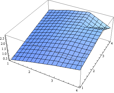
Figure 1. Plot of approximate solution of level $L=1$ for test example.

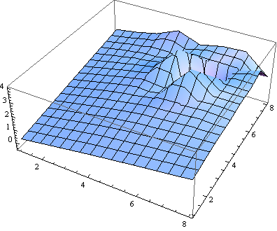
Figure 2. Plot of approximate solution of level $L=2$ for test example.

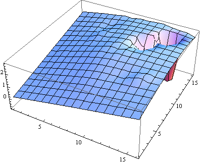
Figure 3. Plot of approximate solution of level $L=3$ for test example.

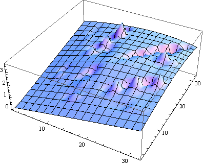
Figure 4. Plot of approximate solution of level $L=4$ for test example.

5. Conclusion

As mentioned above, numerical solution of two-dimensional stochastic integral equations because of the randomness is very difficult or sometimes impossible. In this paper, we have successfully developed Haar wavelets numerical method for approximate a solution of two-dimensional linear stochastic Volterra integral equations. The example confirm that the method is considerably fast and highly accurate as sometimes lead to exact solution. Although, theoretically for getting higher accuracy we can set the method with larger values of M and N and also larger of the degree of approximation, p and q, but it leads to solving MN linear systems of size $pq\times pq$, that have its difficulties. The method can be improved to be more accurate by using other numerical methods. Mathematica has been used for computations in this paper.

References

• [1] I. Aziz, Siraj-ul-Islam, F. Khan, A new method based on Haar wavelet for numerical solution of two-dimensional nonlinear integral equations, J. Comp. Appl. Math. 272 (2014), 70-80.
• [2] I. Aziz, Siraj-ul-Islam, New algorithms for numerical solution of nonlinear Fredholm and Volterra integral equations using Haar wavelets, J. Comp. Appl. Math. 239 (2013) 333-345.
• [3] Siraj-ul-Islam, I. Aziz, M. Fayyaz, A new approach for numerical solution of integro-differential equations via Haar wavelets, Int, J. Comp. Math. 90 (2013) 1971-1989.
• [4] Siraj-ul-Islam, I. Aziz, A. Al-Fhaid, An improved method based on Haar wavelets for numerical solution of nonlinear and integro-differential equations of first and higher orders, J. Comp. Appl. Math. 260 (2014) 449-469.
• [5] Kuo, Hui-Hsiung, Introduction to stochastic integration, Springer Science+Business Media, Inc. 2006.
• [6] K. E. Atkinson, The numerical solution of integral equations of the second kind, Cambridge University Press (1997).
• [7] A. J. Jerri, Introduction to integral equations with applications, John Wiley and Sons, INC (1999).
• [8] T. S. Sankar, V. I. Fabrikant, Investigations of a two-dimentional integral equation in the theory of elasticity and electrostatics, J. Mec. Theor. Appl. 2 (1983) 285-299.
• [9] H. J. Dobner, Bounds for the solution of hyperbolic problems, Computing 38 (1987) 209-218.
• [10] V. M. Aleksandrov, A. V. Manzhirov, Two-dimentional integral equations in applied mechanics of deformable solids, J. Appl. Mech. Tech. Phys. 5 (1987) 146-152.
• [11] A. V. Manzhirov, Contact problems of the interaction between viscoelastic foundations subject to ageing and systems of stamps not applied simultaneously, Prikl. Matem. Mekhan. 4 (1987) 523-535.
• [12] O. V. Soloviev, Low-frequency radio wave propagation in the earth-ionosphere waveguide disturbed by a large-scale three-dimensional irregularity, Radiophysics and Quantum Electronics 41 (1998) 392-402.
• [13] M. Rahman, ”A rigid elliptical disc-inclusion in an elastic solid”, subject to a polynomial normal shift, J. Elasticity 66 (2002) 207-235.
• [14] H. Guoqiang, W. Jiong, Extrapolation of nystrom solution for two dimentional nonlinear Fredholm integral equations, J. Comp. App. Math. 134 (2001) 259-268.
• [15] H. Brunner, Collocation methods for Volterra integral and related functional equations, Cambridge University Press, 2004.
• [16] H. Guoqiang, K. Itayami, K. Sugihara, W. Jiong, Extrapolation method of iterated collocation solution for two-dimentional nonlinear Volterra integral equations, Appl. Math. Comput. 112 (2000) 49-61.
• [17] W. Xie, F. R. Lin, A fast numerical solution method for two dimensional Fredholm integral equations of the second kind, App. Num. Math. 59 (2009) 1709-1719.
• [18] S. Bazm, E. Babolian, Numerical solution of nonlinear two-dimensional Fredholm integral equations of the second kind using Gauss product quadrature rules, Commun. Nonlinear Sci. Numer. Simult. 17 (2012) 1215-1223.
• [19] G. Han, R. Wang, Richardson extrapolation of iterated discrete Galerkin solution for two-dimensional Fredholm integral equations, J. Comp. App. Math. 139 (2002) 49-63.
• [20] K. Maleknejad, Z. JafariBehbahani, Application of two-dimensional triangular functions for solving nonlinear class of mixed Volterra-Fredholm integral equations, Math. Comp. Mode. 55 (2012) 1833-1844.
• [21] E. Babolian, K. Maleknejad, M. Roodaki, H. Almasieh, Two dimensional triangular functions and their applications to nonlinear 2d Volterra-Fredholm equations, Comp. Math. App. 60 (2010) 1711-1722.
• [22] S. Nemati, P. Lima, Y. Ordokhani, Numerical solution of a class of two-dimensional nonlinear Volterra integral equations using legender polynomials, J. Comp. Appl. Math. 242 (2013) 53-69.
• [23] A. Tari, M. Rahimi, S. Shahmorad, F. Talati, Solving a class of two-dimensional linear and nonlinear Volterra integral equations by the differential transform method, J. Comp. Appl. Math. 228 (2009) 70-76.
• [24] P. Assari, H. Adibi, M. Dehghal, A meshless method for solving nonlinear two-dimensional integral equations of the second kind on non-rectangular domains using radial basis functions with error analysis, J. Comp. Appl. Math. 239 (2013) 72-92.
• [25] M. H. Reihani, Z. Abadi, Rationalized Haar functions method for solving Fredholm and Volterra integral equations, J. Comp. Appl. Math. 200 (2007) 12-20.
• [26] F. Hosseini Shekarabi, K. Maleknejad, R. Ezzati, Application of two-dimensional Bernstein polynomials for solving mixed Volterra-Fredholm integral equations, African Mathematical Union and Springer-Verlag Berlin Heidelberg, DOI 10. 1007/s 13370-014-0283-6 2014.
• [27] F. Keinert, Wavelets and Multiwavelets, A Crc Press Company Boca Raton London New York Washington, D. C, 2004.