Schwinger variational principle theory of collisions in the presence of multiple potentials

Abstract

A theoretical method for treating collisions in the presence of multiple potentials is developed by employing the Schwinger variational principle. The current treatment agrees with the local (regularized) frame transformation theory and extends its capabilities. Specifically, the Schwinger variational approach gives results without the divergences that need to be regularized in other methods. Furthermore, it provides a framework to identify the origin of these singularities and possibly improve the local frame transformation. We have used the method to obtain the scattering parameters for different confining potentials symmetric in $x,y$. The method is also used to treat photodetachment processes in the presence of various confining potentials, thereby highlighting effects of the infinitely many closed channels. Two general features predicted are the vanishing of the total photoabsorption probability at every channel threshold and the occurrence of resonances below the channel thresholds for negative scattering lengths. In addition, the case of negative ion photodetachment in the presence of uniform magnetic fields is also considered where unique features emerge at large scattering lengths.

I Introduction

Frame transformation theory constitutes an important theoretical toolkit describing Hamiltonian systems with several potential terms which are dominant in different regions. A particular class of frame transformations, i.e. the local frame transformation (LFT), can provide pivotal insights for quantum mechanical systems which are approximately separable, usually in different coordinates, at small or large distances but are not separable over all space. In their seminal papers, FanoFano (1981) and HarminHarmin (1982a, b, 1981) developed the principles of the LFT theory permitting the theoretical treatment of highly excited alkali atoms in the presence of external electric fields and interpreting on physical grounds the corresponding photoabsorption spectra.

In addition, the unique properties and intuitive insights make the LFT theory the key framework in the investigations of atom-electron collisions under the action of uniform magneticGreene (1987) or electric fieldsWong et al. (1988); Rau and Wong (1988); Greene and Rouze (1988); Slonim and Greene (1991). The description of the corresponding photoabsorption spectra in terms of the LFT approach is accurate even though only a few channels were involved in the actual calculations.

However, in 1966 it was shown that the inclusion of all closed channels yields non-trivial effects when a charged particle is scattered by a zero-range potential in the presence of a magnetic field Demkov and Drukarev (1966). In particular, it was shown that there always exists a bound state for negative scattering length that is collectively supported by all the closed channels (Landau levels) induced by the magnetic field. The properties of this bound state were subsequently investigated in the context of negative-ion photodetachment in weak magnetic fields Grozdanov (1995). However, similar effects also appear in ultracold two-body collisions in tight waveguide geometries yielding confinement-induced resonances of the Fano-Feshbach typeOlshanii (1998). Such scenarios have been studied in terms of LFT theory either for atom-atom scatteringGranger and Blume (2004); Giannakeas et al. (2012); Heß et al. (2014); Zhang and Greene (2013) or dipole-dipole collisionsGiannakeas et al. (2013). LFT theory provided the most complete theoretical framework in order to describe the relevant collisional physics encompassing the concept of infinitely many closed channels. Interestingly, this permitted the theory to go beyond previous studies where the impact of the closed channels is included in an averaging sense Kim et al. (2005); Crawford (1988). However, the integration of the concept of infinitely many closed channels in the LFT approach yielded divergences, which required regularization techniques to be employed to remove the singular behaviorGranger and Blume (2004); Giannakeas et al. (2012); Zhang and Greene (2013); Giannakeas et al. (2013). Evidently, an approach that incorporates the concept of infinitely many closed channels while avoiding the infinities of the LFT treatment could be useful. Such a formalism could provide quantitative insights into the origins of the LFT singularities while preserving the physical intuition of LFT. Also, it could allow the systematic study of non-trivial effects arising from the full Hilbert space in collisional systems, e.g. the scattering of an electron in a Rydberg state from a neutral perturberDu and Greene (1987).

In this paper, a Schwinger variational $K$-matrix approachSchwinger (1947, 1950); Lippmann and Schwinger (1950) is developed for treating Hamiltonians with two potential terms which dominate at different length scales. We restrict our treatment in this paper to the situation of symmetric confining potentials in $x,y$ and no force in $z$; the more general case of asymmetric potentials and/or forces in $z$ will be treated elsewhere. Note that the Schwinger variational principle has been successfully used for the quantitative study of Rydberg moleculesStephens and McKoy (1992), Rydberg atoms Goforth and Watson (1992), electron scatteringLucchese and McKoy (1979); Maleki and Macek (1980) and electron-molecule collisionsLucchese and McKoy (1983); Lino and Lima (2000); Lucchese et al. (1983). However, in most of these studies, the trial function is composed from a superposition of basis functions (often Gaussian orbitals), which requires numerical evaluation of complicated volume integrals. In our analysis, such complications are avoided due to the length scale separation between the two potential terms, permitting us to treat the scattering information analytically.

This paper will focus on the case of a short-range spherically symmetric interaction potential with a confining potential that bounds all the degrees of freedom apart from one at large distances. Note that these types of Hamiltonians refer to the physical systems of atom-atom collisions in tight waveguides or negative ion photodetachment processes in external fields. Under these considerations, the calculations within the Schwinger variational framework are compared to the corresponding regularized LFT derivations for two different confining potentials (a harmonic oscillator and an infinite square well potential), yielding identical results. However, in the current Schwinger variational $K$-matrix approach, the infinitely many closed channels associated with the confining potential produces finite results without regularization.

Our analysis includes several applications of the current formalism to collisions in the presence of either harmonic or infinite square well confining potentials where the corresponding photoabsorption spectra for $s$-wave photoelectrons possesses unique features. Namely, the total photoabsorption probability vanishes at every channel threshold regardless of the specific details of the confining geometries. This threshold phenomenon illustrates the impact of the closed channel physics on the collisional complex. In addition to the cases of harmonic and infinite square well confining potentials, the current development is applied also to infinite rectangular potentials or off-centered scattering in an infinite square well. These particular systems illustrate the physics of infinitely many closed channels in the absence of degeneracies in the spectra of the confining Hamiltonians. As a final application, negative ion photodetachment in the presence of a uniform magnetic field is treated. Note this particular system has been thoroughly investigated both experimentally Larson and Stoneman (1985); Krause (1990) and theoretically Greene (1987); Blumberg et al. (1979); Crawford (1988). However, in most of the theoretical investigations only the open channel physics was considered and this permits us to explicitly show the impact of the closed channels. More specifically, our results are compared to the approximate LFT treatment in Ref. Greene (1987) where only the open channels physics were considered. Qualitative changes occur only near thresholds for small scattering lengths. However, these features are enhanced the cases where the scattering length is comparable to the confinement length scale which implies enormous scattering lengths for laboratory strength magnetic fields or ultrastrong magnetic fields for the usual scattering lengths.

Section II introduces the basic concepts which are used in the rest of this work. Section III focuses on the derivation of the Schwinger variational $K$-matrix for the confining potentials of a harmonic or a square well potential assuming that the short-range spherically symmetric potential induces partial waves with angular and azimuthal quantum numbers $(\ell m)=[(00),(10),(1\pm 1)]$. In addition, connections between the current formalism and the LFT theory are discussed. Section IV is devoted in the discussion of several applications of the Schwinger variational $K$-matrix as well as its comparison with numerical simulations. Several appendices give some of the details of the derivations. Finally Section V summarizes and concludes our analysis.

II Basic definitions and relations

This section contains the conventions used in this paper for the different Hamiltonians with additive potentials, the scattering wave functions as well as the basic scattering parameters (e.g. the $K$-matrix). In addition, the definitions of the corresponding Green’s functions are also included. Since there are many possible conventions, this will allow for unambiguous definitions of parameters.

II.1 Hamiltonians

The scope of this work is to treat the interaction of a particle with different potentials that have qualitatively different character, with the focus on the case where the particle’s motion is unbounded in one direction. The continuum solutions can be obtained and used for the calculation of scattering parameters, photoionization and/or photodetachment cross sections, etc. The full scattering information is encapsulated in the full Hamiltonian $\hat{H}$ which reads:

$$\hat{H}\ket{\psi}=(\hat{H}_{f}+\hat{V})\ket{\psi}=E\ket{\psi},$$ (1)

where $\hat{H}_{f}=p^{2}/2\mu$ is the free particle Hamiltonian and $\mu$ indicates its mass. $\hat{V}$ corresponds to the operator of the total potential, $\ket{\psi}$ is the scattering wave function and $E$ is the total energy.

In the following we assume that the operator $\hat{V}$ in the full Hamiltonian $\hat{H}$ is the sum of two potentials $\hat{V}_{s}$ and $\hat{V}_{c}$, which possess simple functional forms in different coordinate systems. The two potentials are such that the wave function is easily calculated for each potential individually. More specifically, the $\hat{V}_{c}$ will be a smooth potential that extends over large separation distances and affects the asymptotic boundary conditions in $\ket{\psi}$. In this study, the $\hat{V}_{c}$ is considered to bound the motion of the particle in all the degrees of freedom except one. For example, this potential could be a harmonic one, $V_{c}(\mathbf{r})=(\mu/2)\omega_{\perp}^{2}(x^{2}+y^{2})$ with frequency $\omega_{\perp}$, which separates in cylindrical coordinates, or an infinite square well on the $x-y$ plane which separates in Cartesian coordinates. The $V_{s}(\mathbf{r})$ is a potential that is non-zero in a small volume $\tau$ and could be a spherically symmetric potential at the origin.

One key observation concerns the length scale separation between the $\hat{V}_{s}$ and $\hat{V}_{c}$ potential terms. With this assumption in mind two new Hamiltonians are defined which use solely one potential term each. The $\hat{H}_{c}$ is the Hamiltonian that only contains $\hat{V}_{c}$ and does not contain the $V_{s}$.

$$\hat{H}_{c}\ket{\psi_{c}}=E\ket{\psi_{c}},$$ (2)

where $\ket{\psi_{c}}$ is the corresponding wave function and $E$ is the total energy. The solutions are analytic functions and are used in the following to define the asymptotic form of the scattering wave function. In addition, the corresponding collisional information can be expressed in terms of these states.

Consider now the Hamiltonian $\hat{H}_{s}$ which contains only the $\hat{V}_{s}$ potential. Then the corresponding Schrödinger equation reads

$$\hat{H}_{s}\ket{\psi_{s}}=E\ket{\psi_{s}},$$ (3)

where the eigenfunctions of this Hamiltonian have a simple form because they do not include the complicated boundary conditions that arise from the confining potential, $\hat{V}_{c}$. Intuitively, Eq. (3) describes the motion of the particle at small distances where it experiences solely the short-range potential $\hat{V}_{s}$.

II.2 Scattering wave functions and $K$-matrix

In this subsection the scattering wave functions of the $\hat{H}_{s}$ and $\hat{H}_{c}$ Hamiltonians are defined. More specifically, for the Hamiltonian $\hat{H}_{s}$ the corresponding potential term, namely $\hat{V}_{s}$, possesses spherical symmetry and is short-ranged. Therefore, the $\ket{\psi_{s}}$ wave functions in Eq. (3) are expressed in spherical coordinates as radial functions times spherical harmonics. At distances $r>r_{0}$, the $\hat{V}_{s}$ is negligible, namely $V_{s}(r_{0})\approx 0$, therefore the $K$-matrix normalized radial functions are phase-shifted from the free particle wave function according to the following relation:

$$\braket{\mathbf{r}}{\psi_{s}} = \psi_{s,\ell m}(\mathbf{r})$$ (4)

$$= \sqrt{\frac{2\mu k}{\pi\hbar^{2}}}[j_{\ell}(kr)-\tan\delta_{\ell}\leavevmode\nobreak\ n_{\ell}(kr)]Y_{\ell m}(\Omega)$$ (5)

where the parameter $k$ is defined from $E=\hbar^{2}k^{2}/(2\mu)$ and the functions $Y_{\ell m}(\Omega)$ represent the spherical harmonic functions defined at angles $\Omega$. The spherical Bessel [$j_{\ell}(kr)$] and Von Neumann [$n_{\ell}(kr)$] functions correspond to the regular and irregular solutions of the Hamiltonian $\hat{H}_{s}$. The term $\delta_{\ell}$ denotes the phase shift induced by the potential $\hat{V}_{s}$.

In the following, the energy-normalized regular and irregular solutions of the $H_{c}$ Hamiltonian are defined together with the corresponding scattering matrices. The symbol $\psi_{c}$ represents the regular functions at the origin and $\chi_{c}$ represents the irregular functions. Since the $V_{c}$ potential confines the motion in the $x-$ and $y-$directions, then the parity in the $z$-direction, namely $\Pi_{z}$ is a good quantum number and hence the asymptotic form of the regular wave functions are expressed as even and odd solutions

$$\psi^{(e,o)}_{c,\alpha}(\mathbf{r})=\Phi_{\alpha}(x,y)\sqrt{\frac{\mu}{\pi\hbar^{2}k_{\alpha}}}\begin{cases}\cos(k_{\alpha}z),\leavevmode\nobreak\ \leavevmode\nobreak\ \rm{for}\leavevmode\nobreak\ \leavevmode\nobreak\ \Pi_{z}=+1\\ \sin(k_{\alpha}z),\leavevmode\nobreak\ \leavevmode\nobreak\ \rm{for}\leavevmode\nobreak\ \leavevmode\nobreak\ \Pi_{z}=-1,\end{cases}$$ (6)

and the irregular wave functions possess the following form in terms of even and odd solutions

$$\chi^{(e,o)}_{c,\alpha}(\mathbf{r})=\Phi_{\alpha}(x,y)\sqrt{\frac{\mu}{\pi\hbar^{2}k_{\alpha}}}\begin{cases}\sin(k_{\alpha}|z|),\leavevmode\nobreak\ \leavevmode\nobreak\ \rm{for}\leavevmode\nobreak\ \leavevmode\nobreak\ \Pi_{z}=+1\\ -\frac{z}{|z|}\cos(k_{\alpha}|z|),\leavevmode\nobreak\ \leavevmode\nobreak\ \rm{for}\leavevmode\nobreak\ \leavevmode\nobreak\ \Pi_{z}=-1,\end{cases}$$ (7)

where the $\Phi_{\alpha}(x,y)$ are a complete basis of orthonormal eigenfunctions of the transverse part of the $\hat{H}_{c}$ Hamiltonian and their specific form is dictated by the particular type of confining potential $\hat{V}_{c}$. The superscript notation $(e,o)$ in Eqs. (6) and (7) denotes the even ($\Pi_{z}=+1$) and odd ($\Pi_{z}=-1$) solutions, respectively. The total energy is given by the relation $E=\hbar^{2}k_{\alpha}^{2}/2\mu+E_{\alpha}$ where $E_{\alpha}$ is the energy of the transverse function $\Phi_{\alpha}(x,y)$. These equations assume $E>E_{\alpha}$ assuring therefore that the solutions possess an oscillatory behavior. If the $E<E_{\alpha}$, then there are functions that are real exponentials in $z$.

The scattering solutions of the full Hamiltonian $\hat{H}$ at energy $E$ can be expressed at small distances as linear combinations of the eigenfunctions of $\hat{H}_{c}$ Hamiltonian at this same energy $E$. Moreover, if the scattering potential is an even function of $z$, then the solutions separate into sums over the even functions or sums over the odd functions. In this situation, the asymptotic form of the exact wave function of the Hamiltonian $\hat{H}$ can be written as

$$\psi^{(e,o)}_{\alpha}(\mathbf{r}) = \psi^{(e,o)}_{c,\alpha}(\mathbf{r})-\sum_{\beta}\chi^{(e,o)}_{c,\beta}(\mathbf{r})K^{(e,o)}_{\beta\alpha}$$ (8)

where the elements $K^{(e,o)}_{\beta\alpha}$ indicate the $K$-matrix elements of even or odd states in the $z$-direction. The $\alpha,\beta$ indexes label the open channels ($E>E_{\alpha,\beta}$) meaning that the corresponding wave function possess an oscillatory behavior as $|z|\to\infty$. On the other hand asymptotically the closed channels ($E<E_{\alpha}$) are described via the following functions

$$\Upsilon^{(e)}_{\alpha}(\mathbf{r})=\Phi_{\alpha}(x,y)\sqrt{\frac{\mu}{\pi\hbar^{2}\kappa_{\alpha}}}\exp(-\kappa_{\alpha}|z|)$$ (9)

where the index $\alpha$ is here introduce in order to separate the closed from open channels. The energy of the closed channels is given by the relation $E=-\hbar^{2}\kappa_{\alpha}^{2}/2\mu+E_{\alpha}$.

Having specified the scattering eigenfunction of the $\hat{H}_{c}$ Hamiltonian, the corresponding $K$-matrix fulfills the following relation:

$$K_{\alpha\beta}=-\pi\braket{\psi_{c,\alpha}}{\hat{V}_{s}}{\psi_{\beta}}$$ (10)

where $\alpha,\leavevmode\nobreak\ \beta$ label open channels. In addition, the $\ket{\psi_{c}},\leavevmode\nobreak\ \ket{\psi}$ are the exact solutions of $\hat{H}_{c}$ and $\hat{H}$ Hamiltonians, respectively.

Equation (10) can be expressed in a more general way by substituting the exact relation $\hat{V}_{s}\ket{\psi_{\beta}}=(E-\hat{H}_{c})\ket{\psi_{\beta}}$ and integrating by parts twice. Using this, the volume integral in Eq. (10) can be recast as a surface integral that is a simpler expression for the corresponding $K$-matrix:

$$K_{\alpha\beta}^{(e)} = -\frac{\hbar^{2}\pi}{\mu}\int\int W_{z}[\psi^{(e)*}_{c,\alpha}(\mathbf{r}),\psi^{(e)}_{\beta}(\mathbf{r})]dxdy,$$ (11)

where the term $W_{z}[\cdot]$ indicates the Wronskian with respect to the $z$-direction and is evaluated at large enough $|z|$ that the closed functions of Eq. (9) are effectively 0. The closed channels are in the full wave function and could lead to resonances but do not contribute to the surface integrals at large $z$.

II.3 Free particle and confining Green’s functions

The Hamiltonians introduced in Eqs. (2) and (3) permit us to straightforwardly define the two corresponding Green’s functions.

$$\hat{G}_{f}\equiv\frac{1}{E-\hat{H}_{f}}\qquad\hat{G}_{c}\equiv\frac{1}{E-\hat{H}_{c}},$$ (12)

where $\hat{G}_{c}$ only includes the confining potential, and $\hat{G}_{f}$ is the free particle Green’s function for the Hamiltonian with no potential energy. The specific asymptotic boundary conditions in Eq. (12) are determined by how the pole is handled.

The outgoing/incoming free particle Green’s function $\hat{G}_{f}$ in the position representation can be written as

$$\braket{\mathbf{r}_{1}}{\hat{G}^{\pm}_{f}}{\mathbf{r}_{2}}=G_{f}^{\pm}(\mathbf{r}_{1},\mathbf{r}_{2})=-\frac{\mu}{2\pi\hbar^{2}}\frac{e^{\pm ikr_{12}}}{r_{12}},$$ (13)

where $r_{12}=|\mathbf{r}_{1}-\mathbf{r}_{2}|$ and the “$+$” (“$-$”) denotes the outgoing (incoming) Green’s function. The standing wave $G_{f}$ is derived simply by taking the real part of either $G_{f}^{\pm}$.

The outgoing/incoming Green’s function when only the confining potential is present reads

$$\braket{\mathbf{r}_{1}}{\hat{G}^{\pm}_{c}}{\mathbf{r}_{2}} = G_{c}^{\pm}(\mathbf{r}_{1},\mathbf{r}_{2})$$ (14)

$$= \sum_{\alpha=1}^{\alpha_{0}}\frac{\mp i\mu}{\hbar^{2}k_{\alpha}}\Phi^{*}_{\alpha}(\bm{\rho}_{1})\Phi_{\alpha}(\bm{\rho}_{2})e^{\pm ik_{\alpha}|z_{1}-z_{2}|}$$ (15)

$$+ \sum_{\alpha_{0}+1}^{\infty}\frac{\mu}{\hbar^{2}\kappa_{\alpha}}\Phi_{\alpha}(\bm{\rho}_{1})\Phi^{*}_{\alpha}(\bm{\rho}_{2})e^{-\kappa_{\alpha}|z_{1}-z_{2}|},$$ (16)

where $\bm{\rho}$ a vector lying into $x-y$ plane. The index $\alpha_{0}$ denotes the last open channel for a given total energy $E$. As with the $\hat{G}^{\pm}_{f}$, the standing wave $\hat{G}_{c}$ can be obtained from the real part of $\hat{G}_{c}^{\pm}$. Note that this property does not hold in the case of a charged particle motion in magnetic fields.

One important observation is that every Green’s function diverges as $r_{12}\to 0$ in the same way for any energy not at a threshold of $H_{c}$:

$$G_{any}(\mathbf{r}_{1},\mathbf{r}_{2})=-\frac{\mu}{2\pi\hbar^{2}}\frac{1}{r_{12}}+O(r_{12}^{0})$$ (17)

for small $r_{12}$; this result also does not depend on whether the $G$ obeys standing wave or incoming/outgoing boundary conditions. This means the difference of any two Green’s functions is finite everywhere except for energies exactly at threshold. In the expressions below, we will arrange to only have integrals that involve the differences of Green’s functions times functions that are finite and non-zero in a finite region. Thus, our expressions will automatically be finite without the need for regularization procedures.

In this work, the standing wave solutions are employed; therefore the corresponding Green’s functions, i.e. $\hat{G}_{f}$ and $\hat{G}_{c}$ denote the principal value ones.

III Schwinger Variational Principle

This section presents a derivation of the $K$-matrix in terms of the Schwinger variational principle. The main focus of this derivation is the standing wave solution and the corresponding Green’s function. However, note that a similar derivation can be carried out in cases of incoming/outgoing boundary conditions.

Using the Lippmann-Schwinger equation, $\ket{\psi_{\alpha}}=\ket{\psi_{c,\alpha}}+\hat{G}_{c}\hat{V}_{s}\ket{\psi_{\alpha}}$, and its hermitian conjugate in Eq. (10), the following identity for the $K$-matrices is fulfilled

$$K_{\alpha\beta}=-\pi\braket{\psi_{c,\alpha}}{\hat{V}_{s}}{\psi_{\beta}}=-\pi\braket{\psi_{\alpha}}{\hat{V}_{s}}{\psi_{c,\beta}},$$ (18)

where the relation $\hat{G}_{c}^{\dagger}=\hat{G}_{c}$ is used.

A Schwinger-type variational expression for the $K$-matrix can be obtained with the help of Eq. (18) and the trial functions $\ket{\psi^{(\rm{t})}}=\ket{\psi}+\ket{\delta\psi}$ of the full Hamiltonian $H$.

$$K^{\rm{var}}_{\alpha\beta} \equiv -\pi[\braket{\psi_{c,\alpha}}{\hat{V}_{s}}{\psi^{(\rm{t})}_{\beta}}+\braket{\psi^{(\rm{t})}_{\alpha}}{\hat{V}_{s}}{\psi_{c,\beta}}-\braket{\psi^{(\rm{t})}_{\alpha}}{\hat{V}_{s}}{\psi^{(\rm{t})}_{\beta}}$$ (20)

$$+\braket{\psi^{(\rm{t})}_{\alpha}}{\hat{V}_{s}\leavevmode\nobreak\ \hat{G}_{c}\leavevmode\nobreak\ \hat{V}_{s}}{\psi^{(\rm{t})}_{\beta}}],$$

where the variational expression for the $K$-matrix, $K^{\rm{var}}$, equals the exact $K$-matrix, i.e. Eq. (10), plus terms of order $\delta\psi^{2}$:

$$K^{\rm{var}}_{\alpha\beta} = -\pi[\braket{\psi_{c,\alpha}}{\hat{V}_{s}}{\psi_{\beta}}-\braket{\delta\psi_{\alpha}}{\hat{V}_{s}-\hat{V}_{s}\hat{G}_{c}\hat{V}_{s}}{\delta\psi_{\beta}}]$$ (21)

$$= K_{\alpha\beta}+O(\delta\psi^{2})$$ (22)

The trial functions $\ket{\psi^{(\rm{t})}_{\beta}}$ are often written as linear combinations of a basis set of functions $\ket{y_{j}}$.

$$\ket{\psi^{(\rm{t})}_{\beta}}=\sum_{j}\ket{y_{j}}C_{j\beta}.$$ (23)

Substituting Eq. (23) in Eq. (20), the coefficients $C_{j\alpha}$ are specified by requiring Eq. (20) to be variationally stable, i.e. $\partial K_{\alpha\beta}^{\rm{var}}/\partial C_{j\beta}=0$. This yields the basis expansion version of the Schwinger variational expression, $K_{\alpha\beta}^{\rm{var}}$, which reads

$$K^{\rm{var}}_{\alpha\beta}=-\pi\sum_{jj^{\prime}}\braket{\psi_{c,\alpha}}{\hat{V}_{s}}{y_{j}}[M^{-1}]_{jj^{\prime}}\braket{y_{j^{\prime}}}{\hat{V}_{s}}{\psi_{c,\beta}}$$ (24)

where $M_{j^{\prime}j}=\braket{y_{j^{\prime}}}{\hat{V}_{s}-\hat{V}_{s}\hat{G}_{c}\hat{V}_{s}}{y_{j}}$. In addition, the trial functions $\ket{\psi^{(\rm{t})}_{\alpha}}$ can be evaluated via the coefficients $C_{\alpha,j}$ which fulfill the following relation

$$C_{j\beta}=\sum_{j^{\prime}}[M^{-1}]_{jj^{\prime}}\braket{y_{j^{\prime}}}{\hat{V}_{s}}{\psi_{c,\beta}}.$$ (25)

One of the main points of a variational principle is that an exact $K$-matrix is obtained if the $\ket{\psi^{(\rm{t})}}$’s equal the exact $\ket{\psi}$’s. For the Schwinger variational principle, all the corresponding expressions for the $K$-matrix involve terms of $\hat{V}_{s}\ket{\psi^{(\rm{t})}}$. This implies that the exact result for the $K$-matrix is obtained for the Schwinger variational principle even if the $\ket{\psi^{(\rm{t})}}$ satisfies the somewhat looser condition $V_{s}(\mathbf{r})\delta\psi(\mathbf{r})=0$ which will be exploited in the next section.

In particular this condition can be satisfied at large and small distances $r$. At large distances, the potential $\hat{V}_{s}$ vanishes implying that the $\delta\psi(\mathbf{r})$ parts of the trial functions $\ket{\psi^{(\rm{t})}}$ which are nonzero in this region do not contribute to the $K$-matrix calculation. On the other hand, the trial functions at small distances can be chosen such that they are exact solutions of the full Hamiltonian $\hat{H}$ yielding therefore $\delta\psi(\mathbf{r})=0$ at small $r$. This imposes a constraint on the choice of the trial functions or the basis expansions that is employed in the next section. With these choices, the exact $K$-matrix is obtained even if the $\ket{\psi^{(\rm{t})}}$ is not an eigenfunction of the full Hamiltonian $\hat{H}$ over all space.

An additional feature is that if $V_{s}(\mathbf{r})\neq 0$ in a small region of space (and for a limited range of low energies), only the low-$\ell$ angular momentum partial waves of $\ket{\psi^{(\rm{t})}}$ are needed to calculate the $K$-matrix. This holds only away from high-$\ell$ resonances due to the fact that as the angular momentum $\ell$ increases the amplitude of the corresponding wave functions in the region of $V_{s}(\mathbf{r})\neq 0$ vanishes. Therefore, these high-$\ell$ states will not contribute to the scattering information.

IV K-matrix for two potentials: application of the Schwinger variational principle

An important special case is when the potential $\hat{V}_{s}=\hat{H}-\hat{H}_{c}$ is nonzero over a range small enough that the potentials in $\hat{H}_{c}$ Hamiltonian are considered effectively zero (or constant) over the range of $\hat{V}_{s}$. This will allow us to simplify all of the integrals in Eqs. (24) and (25) and in some cases the corresponding results are simple analytic functions. To reduce the amount of new material, we have restricted the scattering systems to have no $z$-dependence to the potential and for the confining potential to have symmetry in $x,y$. Finally, an important consideration for this section is to obtain expressions for the $M$-matrix elements, Eq. (24), as a simple analytic term and a term involving an integral over finite functions.

IV.1 General expression of the K-matrix for short-ranged spherical symmetric potential $\hat{V}_{s}$

As discussed at the end of Sec. III, only low-$\ell$ angular momentum partial waves contribute to the calculation of the $K$-matrix when $\hat{V}_{s}$ is assumed to be short ranged. Therefore, for such a short range potential only the first two angular momentum states will be considered, i.e. $\ell=0$ and $1$. This approximation will allow us to obtain closed form expressions of all the $K$-matrix elements in terms of the $\ell=0$ and $1$ phase shifts.

Since the full potential $\hat{V}$ is symmetric in $z$, the $K$-matrix separates into even- and odd-channel blocks. For each parity state of the $\hat{H}_{c}$ Hamiltonian, only one basis function is used in Eq. (24) which is the solution of $\hat{H}$ Hamiltonian. This will provide the exact scattering information given that the length scale of the potential terms $\hat{V}_{s}$ and $\hat{V}_{c}$ in the full Hamiltonian $\hat{H}$ are well separated. In other words, the length scale separation implies that in the region of $\hat{V}_{s}\neq 0$ the states $\ket{\psi_{s}}$ (see Eq. (3)) will not be modified by the confining potential $\hat{V}_{c}$.

To be precise, if there is a potential that only scatters $s$- and $p$-waves at some specified (low) energy, then the potential only extends over a very short range. The wave function in the region near the scatterer, at position $\mathbf{r}_{s}$, is most easily represented in spherical coordinates. The difficulty will be to evaluate the integrals involving the $\ket{\psi_{c}}$ and the corresponding $\hat{G}_{c}$ which will often be most easily represented in a different coordinate system. The reason that the exact scattering information is obtained from the Schwinger variational principle is that the exact wave function of the full Hamiltonian (including large $r$ boundary conditions) must have the form $\psi(\mathbf{r})=C\psi_{s}(\mathbf{r})+\xi(\mathbf{r})$. Note that $\psi_{s}$ is the spherical wave centered at $r_{s}$ that does not obey the large-$r$ boundary conditions of the full Hamiltonian. The function $\xi=\psi-C\psi_{s}$ only has $\ell\geq 2$ partial waves at $\mathbf{r}_{s}$ which implies $V_{s}(\mathbf{r})\xi(\mathbf{r})=0$ everywhere. This means the exact $K$-matrix can be written as

$$K_{\alpha\beta}=-\pi\frac{\braket{\psi_{c,\alpha}}{\hat{V}_{s}}{\psi_{s}}\braket{\psi_{s}}{\hat{V}_{s}}{\psi_{c,\beta}}}{\braket{\psi_{s}}{\hat{V}_{s}-\hat{V}_{s}\hat{G}_{c}\hat{V}_{s}}{\psi_{s}}},$$ (26)

where each term is now a single matrix element. The terms in the numerator give a finite result because the $\hat{V}_{s}\ket{\psi_{s}}$ is non-zero only over a finite region. Although the term in the denominator is not obviously finite because the $\hat{G}_{c}$ diverges in proportion to $1/|\mathbf{r}_{1}-\mathbf{r}_{2}|$, the derivation below shows that this term can be written as convergent sums.

The evaluation of the term in the denominator of Eq. (26) is complicated by the fact that the $\hat{G}_{c}$ is simple in a different coordinate system from that of $\ket{\psi_{s}}$ and $\hat{V}_{s}$ Stephens and McKoy (1992); Lucchese and McKoy (1979, 1983); Lino and Lima (2000); Lucchese et al. (1983). However, these complications can be avoided by adding and subtracting the Green’s function for a free particle, $\hat{G}_{f}$,

$$\braket{\psi_{s}}{\hat{V}_{s}-\hat{V}_{s}\hat{G}_{c}\hat{V}_{s}}{\psi_{s}}=I_{s}+D_{s}$$ (27)

with the new parameters $I_{s}$ and $D_{s}$ defined as

$$I_{s}=\braket{\psi_{s}}{\hat{V}_{s}-\hat{V}_{s}\hat{G}_{f}\hat{V}_{s}}{\psi_{s}}=-\frac{1}{\pi}\tan\delta_{\ell}$$ (28)

where the $\ket{\psi_{s}}$ indicates a state of a particular angular momentum $\ell$ possessing the form of Eq. (4) and

$$D_{s}=\braket{\psi_{s}}{\hat{V}_{s}\Delta\hat{G}\hat{V}_{s}}{\psi_{s}}=\braket{\psi_{s}}{\hat{V}_{s}(\hat{G}_{f}-\hat{G}_{c})\hat{V}_{s}}{\psi_{s}}$$ (29)

These manipulations have the advantage that the $I_{s}$ is simply related to the no confinement phase shift and the $G_{f}(\mathbf{r}_{1},\mathbf{r}_{2})-G_{c}(\mathbf{r}_{1},\mathbf{r}_{2})$ function is finite for all values of $\mathbf{r}_{1}$ and $\mathbf{r}_{2}$. Thus, the expression in Eq. (29) is finite because the $\hat{V}_{s}\ket{\psi_{s}}$ is finite with a finite range and its square is multiplying a finite function. Note that a similar difference of Green’s functions appears also in the methods presented in Refs.Slonim and Greene (1991); gol (1984) yielding thus finite results.

One important observation is that the $K$-matrix in Eq. (26) is essentially separated in factors of matrix elements. This is crucial since it allows us to treat each factor separately in a pedagogical manner. The following subsections are devoted to providing their explicit analytical expressions.

IV.2 Matrix elements with $\hat{V}_{s}\ket{\psi_{s}}$

It is evident from Eq. (26) that most of the integrals involve terms of $\hat{V}_{s}\ket{\psi_{s}}$; thus this subsection mainly focus on the integrals of the form

$$\braket{\psi_{c}}{\hat{V}_{s}}{\psi_{s}}=\int_{\tau}\psi_{c}(\mathbf{r})V_{s}(\mathbf{r})\psi_{s}(\mathbf{r})d^{3}\mathbf{r},$$ (30)

where $\tau$ is the smallest volume that contains the region where $V_{s}(\mathbf{r})\neq 0$. Recall that the function $\psi_{c}(\mathbf{r})$ is an eigensolution of the $\hat{H}_{c}$ Hamiltonian. Since the $V_{s}(\mathbf{r})$ is nonzero only over a small region, the integral should only be performed over a volume $\tau$ that contains this region.

The Appendix A gives the prescription for evaluating these matrix elements for $\ell\leq 1$. The basic idea is to convert the volume integral into a surface integral which is possible due to the length scale separation between the range of $\hat{V}_{s}$ and when the $\hat{V}_{c}$ becomes non-negligible. The main results are:

$$\braket{\psi^{(e)}_{c,\alpha}}{\hat{V}_{s}}{\psi_{s,00}}=\Phi^{*}_{\alpha}(0,0)\sqrt{\frac{2\pi}{kk_{\alpha}}}\left(-\frac{1}{\pi}\tan\delta_{0}\right)$$ (31)

$$\braket{\psi^{(o)}_{c,\alpha}}{\hat{V}_{s}}{\psi_{s,10}}=\Phi^{*}_{\alpha}(0,0)\sqrt{\frac{6\pi k_{\alpha}}{k^{3}}}\left(-\frac{1}{\pi}\tan\delta_{1}\right)$$ (32)

$$\braket{\psi^{(e)}_{c,\alpha}}{\hat{V}_{s}}{\psi_{s,1\pm 1}}=-(\partial_{\pm}\Phi_{\alpha})^{*}\Bigg{|}_{0}\sqrt{\frac{12\pi}{k_{\alpha}k^{3}}}\left(-\frac{1}{\pi}\tan\delta_{1}\right)$$ (33)

where $(\partial_{\pm}\Phi_{\alpha})\equiv(\partial\Phi_{\alpha}(\mathbf{r})/\partial x\mp i\partial\Phi_{\alpha}(\mathbf{r})/\partial y)/2$.

IV.3 Analytic expressions for the $D_{s}$ matrix elements

This subsection focuses on the $D_{s}$ matrix elements. One of the main assumptions here is that the $\hat{V}_{s}$ potential is centered symmetrically with respect to the confining potential; for example, $\hat{V}_{s}$ is at the origin and $V_{c}(x,y)=V_{c}(y,x)$ and $V_{c}(x,y)=V_{c}(-x,y)$ etc. This allows us to resolve possible challenges with respect to the scattering of $\ell=1,|m|=1$.

The $D_{s}$ matrix elements for $\ell=0,m=0$ and for $\ell=1,\leavevmode\nobreak\ m$ can be written in the compact form

$$D_{s,\ell m}=\left(\frac{1}{\pi}\tan\delta_{\ell}\right)\frac{\tan\delta_{\ell}}{[a_{\perp}k]^{2\ell+1}}\eta_{\ell m}(E)$$ (34)

where the $a_{\perp}$ is a relevant length scale for the confinement potential $\hat{V}_{c}$ and $\eta_{\ell m}(E)$-function is defined in terms of the $\Delta G$ defined in Appendix B. For $\ell=0,\leavevmode\nobreak\ m=0$ and $\ell=1,\leavevmode\nobreak\ m$, they are defined as

$$\eta_{00}(E) = \frac{2\pi\hbar^{2}}{\mu}a_{\perp}\Delta G(0)$$ (35)

$$\eta_{10}(E) = -\frac{6\pi\hbar^{2}}{\mu}a_{\perp}^{3}\Delta G_{zz}(0)$$ (36)

$$\eta_{1\pm 1}(E) = -\frac{6\pi\hbar^{2}}{\mu}a_{\perp}^{3}\Delta G_{\rho\rho}(0)$$ (37)

It is important to note that the expression for $\Delta G$ converges for non-zero $\Delta z$ without the need for regularization. In order to investigate in detail the $\Delta z$ dependence at $\Delta\tilde{\rho}=\frac{\Delta\rho}{a_{\perp}}\ll 1$, the function $\Gamma(\bm{r}_{1},\bm{r}_{2},E)\equiv 2\pi\hbar^{2}a_{\perp}\Delta G(\bm{r}_{1},\bm{r}_{2})/\mu$ is defined which reads

$$\Gamma(\bm{r}_{1},\bm{r}_{2},E)= - 2\pi\sum_{\alpha=1}^{\alpha_{o}}a_{\perp}^{2}\Phi_{\alpha}(\bm{\rho}_{1})\Phi_{\alpha}^{*}(\bm{\rho}_{2})\frac{\sin(\tilde{k}_{\alpha}|\Delta\tilde{z}|)}{\tilde{k}_{\alpha}}$$ (38)

$$+ 2\pi\sum_{\alpha=\alpha_{o}+1}^{\infty}a_{\perp}^{2}\Phi_{\alpha}(\bm{\rho}_{1})\Phi_{\alpha}^{*}(\bm{\rho}_{2})\frac{e^{-\tilde{\kappa}_{\alpha}|\Delta\tilde{z}|}}{\tilde{\kappa}_{\alpha}}$$ (39)

$$- \frac{\cos(\tilde{k}\tilde{r}_{12})}{\tilde{r}_{12}},$$ (40)

where the $E_{\alpha_{o}}<E<E_{\alpha_{o}+1}$ defines the open and closed channels. Parameters with a tilde have been scaled by the length scale $a_{\perp}$ to become dimensionless: $\Delta\tilde{z}=\Delta z/a_{\perp}$, $\tilde{k}=ka_{\perp}$, $\tilde{k}_{\alpha}=k_{\alpha}a_{\perp}$, and $\tilde{\kappa}_{\alpha}=\kappa_{\alpha}a_{\perp}$. In the expression for $\Gamma$, the first term is the contribution from the open channels to $\hat{G}_{c}$, the second term is the contribution from the closed channels to $\hat{G}_{c}$, and the last term is the contribution from $\hat{G}_{f}$.

The three $\eta_{\ell m}(E)$ (see Eq. (35)) functions are derived from the $\Gamma(\bm{r}_{1},\bm{r}_{2},E)$ in the limit $\Delta\tilde{z}\to 0^{+}$ and $\Delta\tilde{\rho}\ll 1$. Physical considerations from Eq. (96) means the expansion of the $\Gamma(\tilde{\mathbf{r}}_{1},\tilde{\mathbf{r}}_{2},E)$ will have the form

$$\Gamma(\bm{r}_{1},\bm{r}_{2},E) \simeq \eta_{00}(E)+\frac{\eta_{10}(E)}{3}\tilde{z}_{1}\tilde{z}_{2}$$ (41)

$$+ \frac{\eta_{11}(E)+\eta_{1-1}(E)}{6}\tilde{\bm{\rho}}_{1}\cdot\tilde{\bm{\rho}}_{2}.$$ (42)

The physical meaning of the $\eta_{\ell m}(E)$ terms is that they encapsulate the impact of the confining geometry, i.e. $\hat{V}_{c}$, on the short-range spherical symmetric potential $\hat{V}_{s}$. Indeed, $\eta_{\ell m}$ conveys the information of each spherical wave of $\ell m$ character induced by the $\hat{V}_{s}$ at short distances is distributed over the asymptotic $\alpha$-channels imposed by $\hat{V}_{c}$ at long distances. Evidently, the explicit form of the $\eta_{\ell m}$ terms depends on the specific type of the confining geometry. Therefore, in the Appendix C, the $\eta_{\ell m}(E)$ terms are evaluated in detail for two types of confining potentials, e.g. the harmonic and the square well potential.

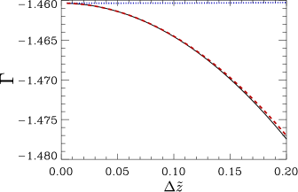
Figure 1: (color online) The quantity $\Gamma$ of Eq. (41) as a function of $\Delta z/a_{\perp}$for the confining potential of the harmonic oscillator infinitesimally above the threshold energy $E=\hbar\omega_{\perp}$ where $\bm{\rho}_{1}=\bm{\rho}_{2}=0$. The black solid line is denotes the sum in Eq. (105). The red dashed line depicts the approximation Eq. (41) using Eq. (56). The blue dotted line indicates a numerical extrapolation of $\Gamma(\bm{r}_{1},\bm{r}_{2},E)\equiv\Gamma(\Delta\tilde{z}\to 0^{+},\Delta\tilde{\rho}\to 0,E)\simeq[4\Gamma(\Delta\tilde{z},0,E)-\Gamma(2\Delta\tilde{z},0,E)]/3$.

IV.4 Test of Taylor series expansion of $\Delta G$

Figure 1 explores the various approximations on the quantity $\Gamma$ which were discussed in Eqs. (38) and (105) considering that the confining potential is a harmonic one. The solid line in Fig. 1 depicts $\Gamma-$quantity from Eq. (38) at energy infinitesimally above the threshold $E=\hbar\omega_{\perp}$ as a function of $\Delta\tilde{z}$ for $\bm{\rho}_{1}=\bm{\rho}_{2}=0$. The latter means that the azimuthal quantum number $m$ is set equal to zero. The red dashed line in Fig. 1 corresponds to Eq. (105) which is obtained by calculating the $\eta_{00}(E)$ and $\eta_{10}(E)$ using the method described in the appendix C. The red dashed and the black solid line are in excellent agreement, especially for small $\Delta\tilde{z}$. This highlights the validity of the approximations that were considered in Eq. (105). In addition, the blue dotted line refers to $\eta_{\ell=0,m=0}(E)$ parameter which is defined as a linear combination of the $\Gamma(\bm{r}_{1},\bm{r}_{2},E)$ functions canceling in this manner terms of the order $|\Delta\tilde{z}|^{2}$ according to the relation $\Gamma(\bm{r}_{1},\bm{r}_{2},E)\equiv\Gamma(\Delta\tilde{z}\to 0^{+},\Delta\tilde{\rho}\to 0,E)\simeq[4\Gamma(\Delta\tilde{z},0,E)-\Gamma(2\Delta\tilde{z},0,E)]/3$. Therefore, in Fig. 1 the dotted, solid and dashed lines converge to the same finite value of $\eta_{\ell=0,m=0}$ without exhibiting any divergences. A similar analysis can be carried out for the $\eta_{\ell=1,m=1}(E)$ and $\eta_{\ell=1,m=\pm 1}(E)$, and it shows excellent convergence between Eqs. (38) and (105).

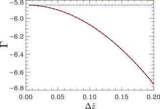
Figure 2: (color online) The quantity $\Gamma$ of Eq. (41) for the square well infinitesimally above the threshold energy $E=\hbar^{2}\pi^{2}/[\mu a_{\perp}^{2}]$ as function of $\Delta\tilde{z}$ for $\bm{\rho}_{1}=\bm{\rho}_{2}=0$. The black solid line denotes the sum in Eq. (117). The red dashed line indicates the approximation Eq. (41) using Eq. (61). The blue dotted line is a numerical extrapolation of $\Gamma(\bm{r}_{1},\bm{r}_{2},E)\equiv\Gamma(\Delta\tilde{z}\to 0^{+},\Delta\tilde{\rho}\to 0,E)\simeq[4\Gamma(\Delta\tilde{z},0,E)-\Gamma(2\Delta\tilde{z},0,E)]/3$.

Similar to Fig. 1, Fig. 2 investigates the validity of Eqs. (38) and (117) for the case of a square well confining potential. Fig. 2 mainly depicts the quantity $\Gamma$ as function of $|\Delta\tilde{z}|$ for $\bm{\rho}_{1}=\bm{\rho}_{2}=0$ infinitesimally above the threshold energy $E=\hbar^{2}\pi^{2}/[\mu a_{\perp}^{2}]$. The black solid line indicates Eq. (38) and the dashed line corresponds to Eq. (117). It is apparent that both relations are in excellent agreement in particular for $\Delta\tilde{z}\to 0$ suggesting in this manner the regime of validity of the Eq. (117). In addition, note that the black solid and the red dashed line converge to the same value as $\Delta\tilde{z}\to 0$, i.e. $\eta_{00}(E)$. Furthermore, the blue dotted line in Fig. 2 consists of a linear combination of the $\Gamma(\bm{r}_{1},\bm{r}_{2},E)$ quantity such that terms of order $|\Delta\tilde{z}|^{2}$ defined by the relation $\Gamma(\bm{r}_{1},\bm{r}_{2},E)\equiv\Gamma(\Delta\tilde{z}\to 0^{+},\Delta\tilde{\rho}\to 0,E)\simeq[4\Gamma(\Delta\tilde{z},0,E)-\Gamma(2\Delta\tilde{z},0,E)]/3$. Evidently, in Fig.2 this linear combination (blue dotted line) is constant in the interval of small $\Delta\tilde{z}$ and corresponds in essence to the value of $\eta_{00}(E)$.

V Scattering observables in terms of the Schwinger variational $K$-matrix

This section utilizes key formulas developed in Section IV in order to explicitly connect the Schwinger variational $K$-matrix of a two potential Hamiltonian with all the relevant scattering observables such as the photoabsorption cross-section. In addition, the transmission and reflection coefficients for quasi-one dimensional Hamiltonians are derived in terms of the Schwinger variational $K$-matrix. This derivations permits us also to discuss the connection of the present study with the theoretical framework of the local frame transformation (LFT) theory. We reiterate that the derivation is for the case of the confining potential being independent of $z$ and symmetric in $xy$; examples that do not follow these restrictions will be presented elsewhere.

V.1 The explicit analytical expressions of the $K$-matrix and its connection with the LFT theory

In this subsection the formulas derived in the subsections IV.2 and IV.3 are the main constituents of the Schwinger variational $K$-matrix in Eq. (26). Recall that the short-range scatterer is assumed to be placed at a symmetry point of the confining potential. This implies that the $K$-matrix will be non-zero in blocks depending on whether the asymptotic channel $\alpha$ couple to $\ell m$ states or not. Note that each $\alpha$-channel is described either by even or odd function in $z$-direction, thus these states couple to $\ell m$ spherically symmetric states if $\ell+m$ is either even or odd, respectively.

In this manner, substituting Eqs. (28), (31) and (34) in Eq. (26) the $K$-matrix is provided for a given $\ell m$ pair of quantum numbers, where the type of confining geometry is not specified. The latter permits us to provide a generic form of scattering matrix elements which read

$$K^{\rm{(e,o})}_{\alpha\beta}=-\mathcal{U}_{\alpha,\ell m}\frac{\tilde{a}_{\ell}^{2\ell+1}(E)}{1+\tilde{a}_{\ell}^{2\ell+1}(E)\eta_{\ell m}(E)}[\mathcal{U}^{\dagger}]_{\ell m,\beta},$$ (43)

where the superscripts $\rm{(e,o)}$ refer to even or odd states in $z$-direction, respectively. Note that the terms $\tilde{a}_{\ell}^{2\ell+1}(E)=a^{2\ell+1}(E)/a^{2\ell+1}_{\perp}$ where $a_{\ell}^{2\ell+1}(E)=-\tan\delta_{\ell}(E)/k^{2\ell+1}$ correspond to $\ell$-wave energy-dependent scattering length ($\ell=0$)or volume ($\ell=1$). It is important to note that for some long range fields, ie. the polarization potential, the scattering volume diverges in the limit of zero total energy. On the other hand, in the problems of the present study the additional confining potential sets a lower limit in the total energy other than zero avoiding in this manner the divergence of the scattering volume. However, in the regime of extremely weak confinement the lower bound in the total energy tends to zero yielding eventually a divergent scattering volume which must be analyzed more carefully. $\eta_{\ell m}(E)$ is the next energy dependent parameter. For specific $\ell m$ state $\eta_{\ell m}(E)$ parameter intrinsically possesses threshold singularities which occur below ($\alpha$)-channel thresholds (see Figs.3 and 4). The matrix elements $\mathcal{U}_{\alpha,\ell m}$ or its conjugate transpose $[\mathcal{U}^{\dagger}]_{\ell m,\alpha}$ capture the coupling of the short- and long-range physics. In other words, the matrix $\mathcal{U}$ contains the information that relates the short-range quantum numbers $\ell$ and $m$ with the $\alpha$ ones which are fully dictated from the confining potential, i.e.. long range physics.

$$\mathcal{U}_{\alpha,\ell m}=\begin{cases}\sqrt{\frac{2\pi a_{\perp}}{k_{\alpha}}}\Phi_{\alpha}(0,0)&\ell=m=0\\ \sqrt{6\pi a_{\perp}^{3}k_{\alpha}}\Phi_{\alpha}(0,0)&\ell=1,\leavevmode\nobreak\ m=0\\ -\sqrt{\frac{12\pi a_{\perp}^{3}}{k_{\alpha}}}(\partial_{\pm}\Phi_{\alpha})\big{|}_{0}&\ell=1,\leavevmode\nobreak\ m=\pm 1\end{cases}$$ (44)

where the operators are defined below Eq. (33).

At this point it becomes evident that Eq. (44) is in essence the local frame transformation (LFT) which permits the the projection of the $\alpha-$states on the $\ell,m$ spherically symmetric states. Note that $\mathcal{U}$ in Eq. (44) and the LFT transformation $U$ in Refs. Greene (1987); Zhang and Greene (2013) are connected according to the relation $\mathcal{U}_{\alpha,\ell m}=U_{\alpha,\ell m}(ka_{\perp})^{\ell+1/2}$. Therefore, specifying the type of the confining potential, i.e. harmonic oscillator or square well, one obtains the local frame transformation either from cylindrical to spherical coordinates Greene (1987) or from Cartesian to spherical coordinates Zhang and Greene (2013). In particular, in Ref. Zhang and Greene (2013), the $\ell=m=0$ derived LFT is identical to Eq. (44). Similarly, the LFT of Ref. Greene (1987) provides the same results as Eq. (44). However, for completeness reasons it should be noted that there is a mistake in Eq. (27) of Ref. Greene (1987), because strictly following the notation of Ref. Greene (1987) would yield the new formula, namely $U_{nl}(m)=U_{q_{n}l}^{\rm{B=0}}(m)(2a)^{1/2}[n!/(n+|m|)!]^{-1/2}[\frac{1}{2}(2n+m+|m|+1)]^{-|m|/2}$.

In addition, the $K$-matrix equation, namely Eq. (43), is exactly the same as the corresponding physical $K$-matrices of Refs.Granger and Blume (2004); Giannakeas et al. (2012); Zhang and Greene (2013). However, there is a conceptual difference between the framework presented here and the framework in Refs.Granger and Blume (2004); Giannakeas et al. (2012); Zhang and Greene (2013). This difference arises from the fact that the $K$-matrices in Refs.Granger and Blume (2004); Giannakeas et al. (2012); Zhang and Greene (2013) did not obey the physical boundary conditions for the closed channels; therefore a closed channel elimination was employed in order to obtain the physical $K$-matrix which obeys the proper boundary conditions. This procedure yield $\eta_{\ell m}(E)$ functions which involve only the sum parts of Eqs. (105) and (117). Thus, the LFT leads to divergences. This singular behavior was removed in a secondary step that required thoughtful implementation of auxiliary techniques of regularization , such as Riemann zeta function regularization Granger and Blume (2004); Giannakeas et al. (2012) or residue regularization Zhang and Greene (2013). On the other hand in the present theoretical framework no such techniques need to be employed since by definition $\eta_{\ell m}(E)$ functions are finite. However, note that $\eta_{\ell m}(E)$ possess intrinsic threshold singularities at energies infinitesimally below the channel thresholds of the confining potential. Furthermore, the Schwinger variational formalism provides an intuitive understanding of the regularization techniques. As is shown in the Appendix C, the $\eta_{\ell m}(E)$ functions consist of a difference of a sum and its integral representation, whereas the latter originates from the free space Green’s function. This piece of information is absent from the physical $K$-matrix in the LFT theory and it is incorporated by various regularization schemes. Perhaps a comparison between the derivation of the LFT and the present results could lead to a deeper understanding of the source of the divergences in the LFT, and deserves to be studied in the future.

V.2 Photoabsorption Cross-section

Since the Schwinger variational $K$-matrix is defined one can also define the electric dipole matrix elements and consequently the photoabsorption cross section. For example, these relations are needed for the treatment of negative ion photodetachment in the present of external fields. Initially, the expression for the trial function coefficients on the basis of the $\ket{\psi_{s}}$, i.e.. Eq. (25) are defined as

$$C_{\ell m,\alpha}=\frac{\mathcal{U}^{\dagger}_{\ell m,\alpha}/[ka_{\perp}]^{\ell+1/2}}{1+\tilde{a}_{\ell}^{2\ell+1}(E)\eta_{\ell m}(E)}.$$ (45)

Since we are interested in computing the cross section that describes, for example, the excitation of a negative ion by photon absorption, the dipole matrix elements at small distances are defined by the relation $D_{lm}(E)=\braket{\psi_{\ell m}}{\hat{\varepsilon}\cdot\hat{r}}{\psi_{\rm{init}}}$. Note that the term $\hat{\varepsilon}\cdot\hat{r}$ is the dipole operator with $\hat{\varepsilon}$ denoting the polarization vector and the state $\psi_{\rm{init}}$ corresponds to the initial state of the negative ion. Having defined the dipole matrix elements at short distances, one can derive the dipole matrix elements that describe the transition from the initial state to the $\alpha-th$ state which includes the confining potential. Therefore, the dipole matrix elements read

$$D_{\alpha}=D_{\ell m}(E)C_{\ell m,\alpha}=\frac{\tilde{D}_{\ell m}(E)\mathcal{U}^{\dagger}_{\ell m,\alpha}}{1+\tilde{a}_{\ell}^{2\ell+1}(E)\eta_{\ell m}(E)}$$ (46)

where the element $\tilde{D}_{\ell m}(E)=D_{\ell m}(E)/(ka_{\perp})^{\ell+1/2}$ typically has less energy dependence than $D_{\ell m}(E)$.

In order to obtain photoabsorption cross sections, we define the dipole matrix elements which describe the transitions from the initial state to the incoming wave final state that possesses only outgoing waves in the $\alpha-th$ channel yielding the following expression:

$$D^{-}_{\alpha}=\sum_{\beta}D_{\beta}[(1-iK)^{-1}]_{\beta\alpha},$$ (47)

where the $K$-matrix has rank one for each $\ell m$ pair, with the relevant eigenvector being proportional to the $D_{\alpha}$. This allows a relatively simple expression for the dipole matrix elements.

$$D^{-}_{\alpha}=\mathcal{U}_{\alpha,\ell m}\frac{\tilde{D}_{\ell m}(E)}{1+\tilde{a}_{\ell}^{2\ell+1}(E)(\eta_{\ell m}(E)-iN_{\ell m}^{2})},$$ (48)

with

$$N_{\ell m}^{2}=\sum_{\alpha=0}^{\alpha_{o}}|\mathcal{U}_{\alpha,\ell m}|^{2}$$ (49)

where the summation index $\alpha$ indicates a sum over only open channels. Then the total probability is proportional to $|D^{-}|^{2}=\sum_{\alpha}|D^{-}_{\alpha}|$ which is the sum over the partial absorption terms $P_{\alpha}=|D^{-}_{\alpha}|^{2}$. The sum reduces to the relation

$$|D^{-}|^{2}=\frac{N_{\ell m}^{2}\tilde{D}_{\ell m}^{2}(E)}{[1+\tilde{a}_{\ell}^{2\ell+1}(E)\eta_{\ell m}(E)]^{2}+[\tilde{a}_{\ell}^{2\ell+1}(E)N_{\ell m}^{2}]^{2}}.$$ (50)

V.3 Transmission and reflection coefficients

This subsection contains expressions for the transmission and reflection coefficients of quasi-one dimensional Hamiltonians in terms of the Schwinger variational $K$-matrix in Eq. (43). This situation models the scattering aspects of two-body collisions in the presence of a transverse harmonic potential or else for collisional complexes of light particles being scattered by heavy ones in the presence of a confining transverse potential.

By superposing the even and odd wave functions, the solution with an incoming wave in the $\alpha-th$ channel can be obtained when $s$- and/or $p$-wave scattering dominates.

$$\psi^{+}_{\alpha}(\mathbf{r}) = \frac{i}{2}\sum_{\beta}\psi_{\beta}^{(o)}(\mathbf{r})[(1-iK^{(o)})^{-1}]_{\beta\alpha}$$ (51)

$$+ \frac{1}{2}\sum_{\beta}\psi_{\beta}^{(e)}(\mathbf{r})[(1-iK^{(e)})^{-1}]_{\beta\alpha},$$ (52)

where the $\psi^{+}_{\alpha}(\mathbf{r})$ only has a wave incoming from negative $z$ in channel $\alpha$. In the case of identical particle collisions having only $s$-wave ($p$-wave) character, the odd (even) $K$-matrix will vanish, namely $K^{(o)}=0$ ($K^{(e)}=0$). On the other hand in the case of distinguishable particles, $s$- and $p$-waves could potentially both be present, and then both even and odd parity $K$-matrices can contribute in the $\psi^{+}_{\alpha}(\mathbf{r})$ wave function.

From the preceding equation one can define the matrices of the corresponding reflection and transmission amplitudes which fulfill the relations

$$r=\frac{iK}{1-iK}\qquad t=\frac{1}{1-iK},$$ (53)

In the case of $s$-wave scattering the reflection and transmission amplitudes can be expressed in terms of the energy dependent scattering length and the matrix $\mathcal{U}$:

$$r_{\beta\alpha} = -\mathcal{U}_{\alpha,00}\frac{i\tilde{a}_{0}(E)}{1+\tilde{a}_{0}(E)(\eta_{00}(E)+iN_{00}^{2})}[\mathcal{U}^{\dagger}]_{00,\beta}$$ (54)

$$t_{\beta\alpha} = \delta_{\beta\alpha}+r_{\beta\alpha}$$ (55)

Note that similar expressions can be obtained for $p$- and $s+p$-wave scattering but it is straightforward to derive them if needed.

From these matrix elements, the scattering probabilities can be obtained. The probability for an incoming wave in channel $\alpha$ to reflect into channel $\beta$ is $|r_{\alpha\beta}|^{2}$ while the probability to transmit into channel $\beta$ is $|t_{\alpha\beta}|^{2}$. Note that the reflection and transmission probabilities are the same except when $\beta=\alpha$. This is understandable on physical grounds: a zero range potential scatters equally into $+z$ and $-z$ but the $\beta=\alpha$ channel has different interference with the incoming wave in the $+z$ and $-z$ directions.

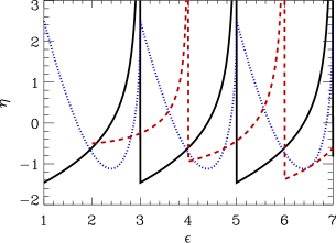
Figure 3: The $\eta_{00}$ (black solid line), $\eta_{10}$ (blue dotted line) and $\eta_{11}/20$ (red dashed line) for harmonic oscillator confinement as a function of the scaled energy $\epsilon=E/(\hbar\omega_{\perp})$.

VI Results and discussion

This section focuses on the various aspects and insights provided by the present framework of the Schwinger variational $K$-matrix approach and its comparison with the LFT results. In addition, a set of selected applications of the current approach is thoroughly discussed to highlight its robustness and clarity. A first test bed is taken to be the study of photodetachment processes in the presence of an external confining field where the closed channel physics is taken into account, thus going beyond previous studies Greene (1987).

Recall that the closed channel physics is fully encapsulated in the $\eta_{\ell m}(E)$ functions which depend on the particular $\ell m$ states of the short range potential and on the specific type of the confining potential.

In other words, $\eta_{\ell m}(E)$ corresponds to a collective parameter, which emerges from the strong mutual coupling of all the closed channels caused by the spherically symmetric short range potential at small distances. In terms of the LFT theory, this collective parameter is described by the eigenvalues of the closed-closed partition of the $K$-matrix and, as was mentioned above, these $K$-matrices are of rank 1 despite the fact that their dimension is $M\times M$ with $M\to\infty$. This particular property ensures that there exists only one nonzero eigenvalue representing the effect of all of the closed channels. Incorporating this concept in photodetachment processes yields non-trivial resonant features; therefore, in the following subsection the energy dependence and broad features of the $\eta_{\ell m}(E)$ functions are studied for various confining potentials.

VI.1 Behavior of $\eta_{\ell m}(E)$

VI.1.1 Harmonic and infinite square well confining potentials

Figures 3 and 4 depict the quantity $\eta_{\ell m}(E)$ as a function of the dimensionless energy $\epsilon$ for the harmonic and infinite square well confining potentials, respectively. Note that the scaled energies $\epsilon$ fulfill the relations $\epsilon=E/\hbar\omega_{\perp}$ and $\epsilon=E/(4\hbar^{2}\pi^{2}/[2\mu a_{\perp}^{2}])$ for the harmonic (Appendix C.1) and square well (Appendix C.2) potentials, respectively.

The expressions for $\eta_{\ell m}$ for the harmonic and square well potential are given in Eqs. (111) and (123), respectively. These parameters are expressed in terms of sums and integrals involving the scaled momenta and $\Delta\tilde{z}$ which can be simplified to show only the dependences on the quantum numbers. For the harmonic oscillator, Eq. (111) becomes

$$\eta_{00} = \sum_{n>\nu_{0}}^{\infty}\frac{e^{-2\sqrt{n-\nu_{0}}\Delta\tilde{z}}}{\sqrt{n-\nu_{0}}}-\int_{\nu_{0}}^{\infty}\frac{e^{-2\sqrt{n-\nu_{0}}\Delta\tilde{z}}}{\sqrt{n-\nu_{0}}}dn$$ (56)

$$\eta_{10} = -12\sum_{n>\nu_{0}}^{\infty}\sqrt{n-\nu_{0}}\;e^{-2\sqrt{n-\nu_{0}}\Delta\tilde{z}}$$ (58)

$$+12\int_{\nu_{0}}^{\infty}\sqrt{n-\nu_{0}}\;e^{-2\sqrt{n-\nu_{0}}\Delta\tilde{z}}dn$$

$$\eta_{1\pm 1} = \sum_{n>\nu_{1}}^{\infty}\frac{(n+1)e^{-2\sqrt{n-\nu_{1}}\Delta\tilde{z}}}{\sqrt{n-\nu_{1}}}$$ (60)

$$-\int_{\nu_{1}}^{\infty}\frac{(n+1)e^{-2\sqrt{n-\nu_{1}}\Delta\tilde{z}}}{\sqrt{n-\nu_{1}}}dn$$

where the limit $\Delta\tilde{z}\to 0^{+}$ is understood in these expressions. $nu_{m}$ is given by $\nu_{m}=(\epsilon-1-|m|)/2$ and it relates with momenta $\tilde{\kappa}_{n,m}$ in Eq. (111) according to the relation $\tilde{\kappa}_{n,m}=2\sqrt{n-\nu_{m}}$. For the square well confinement, Eq. (123) becomes

$$\eta_{00} = 4\sum_{\alpha_{0}^{2}>\epsilon}^{\infty}\frac{e^{-2\pi\sqrt{\alpha_{0}^{2}-\epsilon}\Delta\tilde{z}}}{\sqrt{\alpha_{0}^{2}-\epsilon}}-4\int_{\sqrt{\epsilon}}^{\infty}\frac{e^{-2\pi\sqrt{\alpha^{2}-\epsilon}\Delta\tilde{z}}}{\sqrt{\alpha^{2}-\epsilon}}\frac{\pi}{2}\alpha d\alpha$$ (61)

$$\eta_{10} = -48\pi^{2}\sum_{\alpha_{0}^{2}>\epsilon}^{\infty}\sqrt{\alpha_{0}^{2}-\epsilon}\;e^{-2\pi\sqrt{\alpha_{0}^{2}-\epsilon}\Delta\tilde{z}}$$ (63)

$$+48\pi^{2}\int_{\sqrt{\epsilon}}^{\infty}\sqrt{\alpha^{2}-\epsilon}\;e^{-2\pi\sqrt{\alpha^{2}-\epsilon}\Delta\tilde{z}}\frac{\pi}{2}\alpha d\alpha$$

$$\eta_{1\pm 1} = 48\pi^{2}\sum_{\alpha_{1}^{2}>\epsilon}^{\infty}\frac{(\alpha_{x}+1)^{2}e^{-2\pi\sqrt{\alpha_{1}^{2}-\epsilon}\Delta\tilde{z}}}{\sqrt{\alpha_{1}^{2}-\epsilon}}$$ (65)

$$-48\pi^{2}\int_{\sqrt{\epsilon}}^{\infty}\frac{e^{-2\pi\sqrt{\alpha^{2}-\epsilon}\Delta\tilde{z}}}{\sqrt{\alpha^{2}-\epsilon}}\frac{\pi}{4}\alpha^{3}d\alpha$$

where where the limit $\Delta\tilde{z}\to 0^{+}$ is understood in these expressions. $\alpha_{m}$ is given by $\alpha_{m}^{2}=(\alpha_{x}+[|m|+1]/2)^{2}+(\alpha_{y}+1/2)^{2}$ with $\alpha_{x},\leavevmode\nobreak\ \leavevmode\nobreak\ \alpha_{y}$ independently being $0,1,2,\ldots$. $\alpha_{m}^{2}$ is related with the momenta $\tilde{\kappa}_{\alpha m}$ in Eq. (123) according to the expression $\tilde{\kappa}_{\alpha,m}=2\pi\sqrt{\alpha_{m}^{2}-\epsilon}$. In the integrals, the double integrals $d\alpha_{x}d\alpha_{y}$ have been converted to polar coordinates and the integral over angle from $0$ to $\pi/2$ has been carried out.

Figure 3 shows the results of Eq. (56) for harmonic oscillator confinement for $(\ell m)=[(00),(10),(11)]$ states.

We identify that the parameters $\eta_{00}(E)$ and $\eta_{10}(E)$ from Eq. (56) correspond to the Hurwitz Riemann functions $\zeta(1/2,3/2-E/2\hbar\omega_{\perp})$ and $\zeta(-1/2,3/2-E/2\hbar\omega_{\perp})$, respectively. Note that exactly the same formulas was shown in Refs.Olshanii (1998); Granger and Blume (2004). Furthermore, as was shown also in Ref. Hess et al. (2015), the $\eta_{00}(E)$ (see black solid line in Fig.3) and $\eta_{10}(E)$ (see blue dotted line in Fig.3) are periodic functions of $\epsilon=E/(\hbar\omega)$: $\eta_{\ell m}(\epsilon+2)=\eta_{\ell m}(\epsilon)$.

However, the $\eta_{11}(E)$ function (see red dashed line in Fig.3) starts at a higher threshold energy because the lowest transversal state for $m=1$ is an $\hbar\omega$ higher in energy than for $m=0$ and it is not periodic in $\epsilon$. Actually, the $\eta_{11}(E)$ consists of a sum of the periodic functions $\eta_{00}(E)$ and $\eta_{10}(E)$. However, the corresponding $\eta_{00}(E)$ term is proportional to the energy, which explains the non-periodic character of $\eta_{11}(E)$.

The $\eta_{00}$ and $\eta_{1\pm 1}$ functions diverge as the energy approaches a channel from below due to threshold singularities whereas the $\eta_{10}$ remains finite at each channel threshold. More specifically, the $\eta_{00}$ and $\eta_{1\pm 1}$ diverge due to the terms of the $1/\kappa_{\alpha}$ in the summation whereas the $\eta_{10}$ does not exhibit such features at threshold because the summation involves terms proportional to $\kappa_{\alpha}$. Furthermore, at each threshold, the value $\eta_{10}=2.494632...$ which is the same as in Refs. Granger and Blume (2004); Heß et al. (2014). Similarly, the $\eta_{00}$ parameter acquires the value $\eta_{00}=-1.460354...$ by approaching the thresholds from above which is the same as in Refs. Demkov and Drukarev (1966); Olshanii (1998). The $\eta_{11}$ function has the values $\eta_{11}=-10.00944$ at the lowest threshold and $-18.77157$ at the first excited threshold when approaching those thresholds from above. On the other hand, when the threshold is approached from below the $\eta_{11}$ function diverges and this behavior arises from the singular behavior of the $\eta_{00}$.

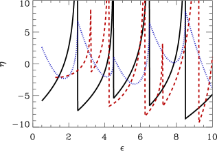
Figure 4: The $\eta_{00}$ (black solid line), $\eta_{10}/50$ (blue dotted line) and $\eta_{11}/300$ (red dashed line) for infinite square well confinement as a function of the scaled energy $\epsilon=E/(4\hbar^{2}\pi^{2}/[2\mu a_{\perp}^{2}])$.

Figure 4 illustrates the $\eta_{\ell m}(E)$ functions for the infinite square well potential where $(\ell m)=[(00),(10),(11)]$ states are considered. More specifically, the functions $\eta_{00}$ (black solid line), $\eta_{10}/50$ (blue dotted line) and $\eta_{11}/300$ (red dashed line) are shown versus the scaled energy $\epsilon=E/(4\hbar^{2}\pi^{2}/[2\mu a_{\perp}^{2}])$. In contrast to Fig. 3, none of the $\eta$’s are periodic functions of $\epsilon$. As with Fig. 3, the $\eta_{00}$ and $\eta_{11}$ go to $\infty$ as the thresholds are approached from below whereas they acquire a finite negative value as the thresholds are approached from above. This behavior arises from a similar analysis to that for Fig. 3 but now involving the individual terms in Eq. (61). As in the harmonic oscillator example, $\eta_{11}$ starts at a higher threshold energy because the transverse functions must have a node to contribute, since the azimuthal quantum number is $m=1$. Our threshold value for $\eta_{00}=-5.853459...$ is in excellent agreement with Ref. (Zhang and Greene, 2013) result from the R-matrix calculation but is $\sim 0.2$% different from the result of their regularized analytical summation. In addition, from Fig. 4 the threshold values of the functions $\eta_{10}$ and $\eta_{11}$ acquire the values $\eta_{10}=132.098...$ and $\eta_{11}=-642.613...$, respectively. Note that $\eta_{10}$ has been divided by a factor of 50 and $\eta_{11}$ by a factor of 300 to plot them on the same graph. This indicates that the effect of the confinement on $p$-wave scattering will typically be larger for the infinite square well than for the harmonic oscillator.

VI.1.2 Infinite Rectangular Well Confinement

Due to the simplicity of the current formalism one can explore the properties of various confining geometries. In this section, the case of a rectangular well confinement is considered. This particular geometry permits us to study the impact of lifting the degeneracy of the square-well potential. Furthermore, in the following the discussion is restricted on $s$-wave scattering which couples only on even $z$-parity states of the rectangular well and/or on $p$-wave collisions which couples odd $z$-parity states of the rectangular well.

The rectangular potential well is defined as follows: $V(x,y)=0$ when $|x|<a_{\perp}/2$ and $|y|<a_{\perp}/(2c)$ and $V(x,y)=\infty$ otherwise. Note that the parameter $c$ controls the degree of asymmetry in the potential. The transverse eigenfunctions of the corresponding confining Hamiltonian $\hat{H}_{c}$ are well known and close to the origin obey the relation

$$\Phi_{\alpha_{x},\alpha_{y}}(0,0)=\frac{2(-1)^{\alpha_{x}+\alpha_{y}}}{a_{\perp}\sqrt{c}}$$ (66)

for all $(\alpha_{x},\alpha_{y})$ that are non-zero at the origin. The corresponding eigenenergies for the states that are nonzero at the origin can be written as

$$E_{n_{x}n_{y}}=\frac{\hbar^{2}\pi^{2}}{2\mu a_{\perp}^{2}}(n_{x}^{2}+[n_{y}/c]^{2})$$ (67)

where $n_{x}=2\alpha_{x}+1$ and $n_{y}=2\alpha_{y}+1$ where the $\alpha_{x},\alpha_{y}$ can independently be $0,1,2,3,...$.

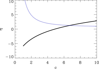
Figure 5: (color online) The threshold value of $\eta_{00}$ (black solid line) and $\eta_{10}/10$ (blue dotted line) for the infinite rectangular well as a function of the ratio of confining length scales, $c$ defined as $|x|<a_{\perp}/2$ and $|y|<a_{\perp}/(2c)$. Note $\eta_{00}$ goes from negative to positive at $c\simeq 4.89$.

Since we are interested in $s-$ and $p$-wave scattering which respectively couple to even and odd-parity states of the rectangular well the prescription given in the appendix C.2 is followed in order to obtain the corresponding parameters. Namely, the $\eta_{00}$ and $\eta_{10}$ parameters fulfill the following relations:

$$\eta_{00} = \frac{4}{c}\sum_{\alpha_{0}^{2}>\epsilon}^{\infty}\frac{e^{-2\pi\sqrt{\alpha_{0}^{2}-\epsilon}\Delta\tilde{z}}}{\sqrt{\alpha_{0}^{2}-\epsilon}}-4\int_{\sqrt{\epsilon}}^{\infty}\frac{e^{-2\pi\sqrt{\alpha^{2}-\epsilon}\Delta\tilde{z}}}{\sqrt{\alpha^{2}-\epsilon}}\frac{\pi}{2}\alpha d\alpha$$ (68)

$$\eta_{10} = \frac{-48\pi^{2}}{c}\sum_{\alpha_{0}^{2}>\epsilon}^{\infty}\sqrt{\alpha_{0}^{2}-\epsilon}\;e^{-2\pi\sqrt{\alpha_{0}^{2}-\epsilon}\Delta\tilde{z}}$$ (70)

$$+48\pi^{2}\int_{\sqrt{\epsilon}}^{\infty}\sqrt{\alpha^{2}-\epsilon}\;e^{-2\pi\sqrt{\alpha^{2}-\epsilon}\Delta\tilde{z}}\frac{\pi}{2}\alpha d\alpha$$

where where the limit $\Delta\tilde{z}\to 0^{+}$ is understood in these expressions and $\alpha_{0}$ obeys the relation $\alpha_{0}^{2}=(\alpha_{x}+1/2)^{2}+(\alpha_{y}+1/2)^{2}$. In the integrals, the double integrals $d\alpha_{x}d\alpha_{y}$ have been converted to polar coordinates and the integral over angle from $0$ to $\pi/2$ has been carried out. Our numerical tests demonstrate that the resulting equations for $\Gamma$ and $\eta_{00}$,$\eta_{10}$ are in agreement and produce results similar to those shown in Fig. 1 and 2. The expressions in Eq. (68) use the fact that the sums and integrals coincide in the continuum limit. To see that this is the case, note that the sums in $\alpha_{y}$ have a factor of $c$ more states for each interval of energy which cancel the factor of $1/c$ multiplying each sum.

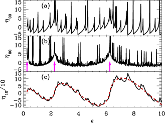
Figure 6: (color online) The $\eta_{00}$ parameter is depicted in panels (a) and (b) for $c=5$ and $c=40$, respectively. The $\eta_{10}/10$ parameter is depicted in panel (c) for $c=5$ (black solid line), and $c=40$ (red dashed line). All the $eta$-parameters are plotted as a function of the scaled energy $\epsilon=E/(4\hbar^{2}\pi^{2}/[2\mu a_{\perp}^{2}])$. The magenta arrows in panel (b) show the thresholds for the tight confinement in one direction, ie $c\gg 1$, which acquire the values $\epsilon=1/4$, $9/4$, $25/4$, …

Figure 5 shows the $\eta_{00}$ (black solid line) and $\eta_{10}/10$ (blue dotted line) from Eq. (68) as a function of the ratio of $y$- to $x$-length scale at the threshold energy $E=E_{1,1}$. The $\eta_{10}$ stays positive for the values shown but the $\eta_{00}$ changes sign for $c\simeq 4.89$. At this value of $c$, the effect of the infinite closed channels disappears for any finite value of the scattering length. In other words, the scattering behaves as if there were no confining potential at all; a similar effect also exists in the harmonic oscillator confining potential which occurs at specific values of energies away from the channel thresholds Heß et al. (2014). Over the range shown in Fig.6 at large values of $c$ the threshold value of $\eta_{00}$ appears to be proportional to $\sqrt{c}$ while the $\eta_{10}$ appears to be a constant plus a function proportional to $1/\sqrt{c}$.

Figure 6 depicts the energy dependence of $\eta_{00}$ and $\eta_{10}/10$ parameters for different values of $c$. As $c$ becomes larger, the corresponding Hamiltonian changes from a quasi-one dimensional to a quasi-two dimensional one. Since the $\eta_{00}$ diverges just below each threshold, these curves exhibit many points of divergence corresponding to each threshold. However, an overall pattern can be seen in panels (b) and (c). This pattern is clearer in the plot of $\eta_{10}/10$ [see red dashed line in Fig.6(c)] which does not diverge at threshold. In Figs.6 (a) and (b) the $c$ parameter acquires the values $c=5$ and $c=40$. In these panels is observed that as $c$ increases the system behaves more like it is only confined in the $x$-direction and therefore those thresholds [see the magenta arrows at $\epsilon=1/4$, $9/4$, $25/4,\ldots$ if Fig.6(b)] dominantly characterize the energy dependence in the corresponding $\eta_{00}$ functions. Moreover, Fig.6(b) demonstrates that the multiple divergences of the $\eta_{00}$ parameter occur around an envelope curve. This overall behavior can be captured by defining an averaged $\eta_{00}$ according to the relation

$$\braket{\eta_{00}}=\frac{1}{2\delta\nu}\int_{\nu-\delta\nu}^{\nu+\delta\nu}\eta_{00}(\nu)d\nu$$ (71)

which will give a smooth curve in the limit that the energy spacing is smaller than $\delta\nu$.

VI.1.3 Off-center scattering for a square well confining potential

The above results for the infinite square and infinite rectangular wells are based on the assumption that the scattering center, i.e. the short-range potential $\hat{V}_{s}$, is placed at the center of the confining potential. In this section, the confining potential is considered to be an infinite square well where the scattering center is located at a generic point, $(x_{s},y_{s})=a_{\perp}(\tilde{x}_{s},\tilde{y}_{s})$ whereby the transverse wave function $|\Phi(x_{s},y_{s})|$ is no longer only 0 or $2/a_{\perp}$ as in the previous cases with $(x_{s},y_{s})=(0,0)$. Note that similar systems have been investigated where the interacting particles are confined in separate harmonic waveguide geometries yielding in this manner confinement-induced interlayer molecules Kanász-Nagy et al. (2015).

In the following, the discussion restricted on $s-$wave scattering which couples on even $z$-parity states of the confining square well and/or $p$-wave collisions which couple on odd $z$-parity states of the corresponding confining potential.

In this case the eigenenergies are defined as follows:

$$E_{n_{x}n_{y}}=\frac{\hbar^{2}\pi^{2}}{2\mu a_{\perp}^{2}}(n_{x}^{2}+n_{y}^{2})$$ (72)

but now the $n_{x}$ and $n_{y}$ can independently be $1,2,3$. The one dimensional wave function is $\psi(x)=\sqrt{2/a_{\perp}}\sin(n_{x}\pi[\tilde{x}-1/2])$. The transverse eigenfunction of the corresponding confining Hamiltonian $\hat{H}_{c}$ at the scattering center behave as

$$\Phi_{\alpha}(x_{s},y_{s})=\frac{2}{a_{\perp}}\sin(\tilde{k}_{x}[\tilde{x}_{s}-1/2])\sin(\tilde{k}_{x}[\tilde{y}_{s}-1/2])$$ (73)

where $\tilde{k}_{x}=n_{x}\pi$ and $\tilde{k}_{y}=n_{y}\pi$. The only nonzero terms when the scattering center is at the origin is from the $n_{x}$ and $n_{y}$ which are the odd integers.

For the case of $s$-wave scattering which couples on even $z-$parity states of the square well and for the case of $p$-wave scattering which couples on odd $z$-parity states the prescription given in the appendix C.2 defining in this manner the corresponding $\eta$-parameters. Namely, the $\eta_{00}$ and $\eta_{10}$ functions fulfill the following relations:

$$\eta_{00}= 4\sum_{\alpha_{0}^{2}>\epsilon}^{\infty}R_{n_{x},n_{y}}(\tilde{x}_{s},\tilde{y}_{s})\frac{e^{-2\pi\sqrt{\alpha_{0}^{2}-\epsilon}\Delta\tilde{z}}}{\sqrt{\alpha_{0}^{2}-\epsilon}}$$ (75)

$$-4\int_{\sqrt{\epsilon}}^{\infty}\frac{e^{-2\pi\sqrt{\alpha^{2}-\epsilon}\Delta\tilde{z}}}{\sqrt{\alpha^{2}-\epsilon}}\frac{\pi}{2}\alpha d\alpha$$

$$\eta_{10}=- 48\pi^{2}\sum_{\alpha_{0}^{2}>\epsilon}^{\infty}R_{n_{x},n_{y}}(\tilde{x}_{s},\tilde{y}_{s})\sqrt{\alpha_{0}^{2}-\epsilon}\;e^{-2\pi\sqrt{\alpha_{0}^{2}-\epsilon}\Delta\tilde{z}}$$ (77)

$$+48\pi^{2}\int_{\sqrt{\epsilon}}^{\infty}\sqrt{\alpha^{2}-\epsilon}\;e^{-2\pi\sqrt{\alpha^{2}-\epsilon}\Delta\tilde{z}}\frac{\pi}{2}\alpha d\alpha,$$

with

$$R_{n_{x},n_{y}}(\tilde{x}_{s},\tilde{y}_{s})=\frac{a^{2}_{\perp}}{4}|\Phi_{\alpha}(x,y)|^{2}$$ (78)

$$\hbox{}\hbox{}\hbox{}\leavevmode\nobreak\ \leavevmode\nobreak\ \leavevmode\nobreak\ \leavevmode\nobreak\ \leavevmode\nobreak\ \leavevmode\nobreak\ \leavevmode\nobreak\ \leavevmode\nobreak\ \leavevmode\nobreak\ \leavevmode\nobreak\ \leavevmode\nobreak\ \leavevmode\nobreak\ \leavevmode\nobreak\ \leavevmode\nobreak\ \leavevmode\nobreak\ \leavevmode\nobreak\ \leavevmode\nobreak\ \leavevmode\nobreak\ =\sin^{2}(\tilde{k}_{x}[\tilde{x}-1/2])\sin^{2}(\tilde{k}_{y}[\tilde{y}-1/2]).$$ (79)

where $\alpha_{0}^{2}=(n_{x}/2)^{2}+(n_{y}/2)^{2}$. In the integrals, the double integrals $d\alpha_{x}d\alpha_{y}$ have been converted to cylindrical coordinates and the integral over angle from $0$ to $\pi/2$ has been carried out. It may appear that these expressions do not satisfy the condition that the sum and the respective integral should have the same form in order for their divergences to cancel and leave a finite difference. To see that the condition still holds, note that the sum is over 4 times as many terms as the centered square well, but the average value of $R_{n_{x},n_{y}}(\tilde{x}_{s},\tilde{y}_{s})$ is 1/4. Numerically tests have confirmed that the resulting equations for $\Gamma$ and $\eta_{00}$,$\eta_{10}$ exhibit excellent agreement, and they depict features similar to those shown in Figs. 1 and 2.

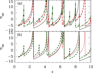
Figure 7: (color online) The parameter $\eta_{00}$ for infinite square well confinement is shown as a function of the scaled energy $\epsilon=E/(4\hbar^{2}\pi^{2}/[2\mu a_{\perp}^{2}])$ with the scattering center at the scaled position $(\tilde{x}_{s},\tilde{y}_{s})$: Panel (a) $(0.0,0.0)$ is the black solid line, $(0.1,0.1)$ is the red dot-dash line, and $(0.2,0.2)$ is the green dot-dot-dot-dash line. Panel (b) $(0.0,0.0)$ is the black solid line, $(0.1,0.0)$ is the red dotted line, $(0.2,0.0)$ is the green dashed line. The solid line is the same result as in Fig.4.

Figure 7 depicts the $\eta_{00}$ function for different positions of the scattering center: $(\tilde{x}_{s},\tilde{y}_{s})$. As in Fig. 4, the quantity $\eta_{00}$ is singular as the energy approaches thresholds from below. In addition, Fig. 7 demonstrates that there are many more thresholds when the scattering center is shifted from the origin. This is due to the possibility of scattering into states that have a node at the origin. In discussing the position of thresholds, we will only give the values for $n_{x}\leq n_{y}$. The black solid line in panels (a) and (b) refers to the position $(0,0)$ and is the same result as plotted in Fig. 4. At this position, there are only singularities at the values of $n_{x},n_{y}$ equal to odd integers. The thresholds in Fig. 7 are 1,3 at $\epsilon=2.5$, 3,3 at $\epsilon=4.5$, 1,5 at $\epsilon=6.5$, and 3,5 at $\epsilon=8.5$. In Fig.7(b) the $\eta_{00}$ parameter is shown for a scattering center being placed along the $x$-axis, namely at $(0.1,0.0)$ (red dotted line) and $(0.2,0.0)$ (green dashed line) can have additional singularities than in the case of a scatterer placed at the origin [see black solid line in Fig.7(b)]. Specifically, the additional structure emerges when one of $n_{x}$,$n_{y}$ is an even integer. The additional singularities over those for the scatterer at the center are for $1,2$ at $\epsilon=1.25$, for $2,3$ at $\epsilon=3.25$, for $1,4$ at $\epsilon=4.25$, for $3,4$ at $\epsilon=6.25$, for $2,5$ at $\epsilon=7.25$, and for $1,6$ at $\epsilon=9.25$. In Fig.7(a) the $\eta_{00}$ parameter is shown for a scattering center being placed along the diagonal of the $x-y$ plane, namely at $(0.1,0.1)$ (red dot-dash line) and $(0.2,0.2)$ (green dot-dot-dot-dash line) where both curves possess additional threshold singularities in comparison with the black solid line and the curves in Fig. 7(b). Specifically, the additional structure emerges when both $n_{x},n_{y}$ are even integers. The additional threshold singularities are for $2,2$ at $\epsilon=2$, for $2,4$ at $\epsilon=5$, for $4,4$ at $\epsilon=8$ and for $2,6$ at $\epsilon=10$.

The coefficient of the diverging term is proportional to $R_{n_{x},n_{y}}$ and, thus, has different effect depending on the value of the transverse function at the scattering center that corresponds to that threshold. For example, the divergence at $\epsilon=2$ (corresponding to 2,2) is clearly visible when the scattering center is at $(0.2,0,2)$ but is not visible when the center is at $(0.1,0.1)$. This is because the latter position is not far shifted from the origin so that it is still near enough to the node of the transverse function to be suppressed. The divergence at $\epsilon=5$ (corresponding to 2,4) is visible in both because the larger quantum number increases the amplitude of the transverse function at the point $(0.1,0.1)$. Another interesting feature is that the divergence at $\epsilon=4.25$ corresponding to $1,4$ has a large strength partly because it is near the divergence at $\epsilon=4.5$ corresponding to 3,3.

There are similar types of features in the plots of $\eta_{10}$. However, because $\eta_{10}$ does not diverge at thresholds, there are discontinuities in slope at the newly allowed thresholds.

VI.2 Photoabsorption cross section in a harmonic and square well confining geometries

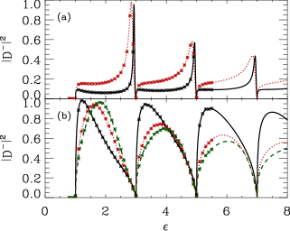
Figure 8: (color online) The total absorption probability $|D^{-}|^{2}$ (in arbitrary units) for a harmonic oscillator confining potential as a function of the scaled energy, $\epsilon=E/(\hbar\omega_{\perp})$. The lines correspond in calculations using Eq. (50) with $(\ell,m)=(0,0)$. The symbols refer to the ab initio quantum calculations using coupled angular momenta for the energy range $0.9\leq\epsilon\leq 5.5$. In panel (a) the $s$-wave scattering lengths take the values of $-a_{\perp}/4$ (black solid line) and $-a_{\perp}/2$ (red dotted line). In panel (b) the $s$-wave scattering lengths refer to values of $a_{\perp}/4$ (black solid line), $a_{\perp}/2$ (red dotted line), and $0.68475a_{\perp}$ (green dashed line).

This subsection investigates the impact of the transversally harmonic or square well confining potentials on the photoabsorption cross sections. In Fig. 8, the absorption probability is plotted as a function of the scaled energy $\epsilon=E/\hbar\omega_{\perp}$ for the harmonic oscillator confining potential. The different plots are for different scattering lengths for $(\ell,m)=(0,0)$. This figure has both lines and symbols. The lines are from Eq. (50) while the symbols are from an ab initio quantum calculation that used a grid in $r$ and angular momentum to compute the total outgoing flux. The only adjustment between the two types of calculations was an overall scale size. The good agreement between the two types of calculations shows that Eq. (50) is an excellent approximation.

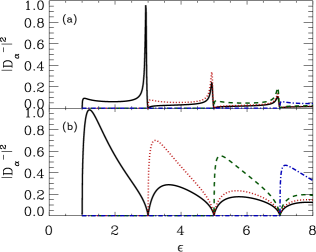
Figure 9: (color online) The partial absorption probability, $|D_{\alpha}^{-}|^{2}$ (in arbitrary units) for a harmonic oscillator confining potential in arbitrary units as a function of the scaled energy, $\epsilon=E/(\hbar\omega_{\perp})$. The lines are calculations using Eq. (50) with $(\ell,m)=(0,0)$. Panels (a) and (b) correspond to $s$-wave scattering lengths of $-a_{\perp}/4$ and $a_{\perp}/4$, respectively. The black solid line is for absorption into the 1st open channel, red dotted line is 2nd open channel, green dashed line is 3rd open channel, and blue dot-dashed line is 4th open channel.

Two interesting features are worth noting. The most obvious feature is that the total probability goes to 0 at every threshold. The probability goes to zero as the threshold is approached from below and from above. As the energy approaches a channel threshold from below, the parameter $\eta_{00}\to\infty$ which means that $|D^{-}|^{2}\to 0$ since the $\eta_{00}$ is in the denominator of $|D^{-}|^{2}$. As the energy approaches a channel threshold from above, $N_{00}^{2}\to\infty$ because the corresponding channel momentum vanishes, namely $k_{\beta}\to 0$. In the expression for $|D^{-}|^{2}$, there is an $N_{00}^{2}$ in the numerator and an $N_{00}^{4}$ in the denominator yielding $|D^{-}|^{2}\to 0$. The total absorption probability is proportional to $\sqrt{|E-E_{\alpha}|}$ at each channel threshold $E_{\alpha}$. This behavior is in strong contrast to the unconfined absorption probability where there is a discontinuity in the slope at each channel threshold, but the total absorption does not go to zero at each threshold. Also, in the case of confinement, the photoabsorption probabilities possess discontinuous slopes near the channel thresholds.

Another important feature is that a negative scattering length causes a resonance-like structure just below each channel threshold [see Fig.8(a)]. On the other hand in Fig.8(b) no resonant structure emerges below each threshold if the $s$-wave scattering length is positive. This behavior can be understood by the fact that for negative $s$-wave scattering lengths the term $1+a_{s}(E)\eta_{00}(E)$ in the denominator of the total absorption probability vanishes yielding in this manner a maximum in the total probability. This effect clearly originates from the closed channel physics. In addition, in Fig.8(a) we observe that for smaller (in magnitude) values of scattering length, the resonance occurs closer to threshold and is narrower in energy. This is to be expected because the smaller (in magnitude) scattering length corresponds to a state that is more weakly bound and, hence, a smaller overlap with the scattering center leading to a longer lifetime and narrower resonant features.

Figure 9 depicts the partial absorption probability $|D_{\alpha}^{-}|^{2}$ for a negative [see Fig.9(a)] and a positive $s$-wave scattering length [see Fig.9(b)] case. The partial cross section is proportional to $|\mathcal{U}_{\alpha,00}|^{2}$ which is proportional to $1/k_{\alpha}$ since the $\Phi_{\alpha}(0,0)$ has no dependence on the $\alpha$ channel quantum number. The channel momentum $k_{\alpha}$ decreases with increasing $\alpha$ which means the partial cross section increases with increasing $\alpha$. Also, the partial absorption cross section exhibits differences between channels just above a channel threshold as it is demonstrated in Fig. 9, i.e. in panels (a) and (b) for the energy interval $3<\epsilon<5$ the $|D_{\alpha}^{-}|^{2}$ of the second channel (red dotted line) is larger than the partial photoabsorption in the first channel. In this case, the channel that just opened will have $k_{\alpha}\sim 0$ and will therefore have nearly all of the outgoing probability.

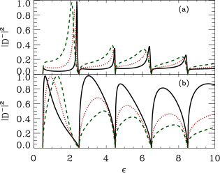
Figure 10: (color online) The total absorption probability $|D^{-}|^{2}$ (in arbitrary units) for an infinite square well confining potential in arbitrary units as a function of the scaled energy $\epsilon=E/(4\hbar^{2}\pi^{2}/[2\mu a_{\perp}^{2}])$ with $(\ell,m)=(0,0)$. The lines refer to calculations based on Eq. (50). In panel (a) the $s$-wave scattering lengths acquire the values $-a_{\perp}/16$ (black solid line), $-a_{\perp}/8$ (red dotted line) and $-a_{\perp}/4$ (green dashed line). In panel (b) the $s$-wave scattering lengths have the values $a_{\perp}/16$ (black solid line), $a_{\perp}/8$ (red dotted line) and $a_{\perp}/4$ (green dashed line).

Figure 10 demonstrates the cases of total absorption probabilities for the infinite square well case for negative [see Fig. 10(a)] and positive [see Fig. 10(b)] $s$-wave scattering lengths. The black solid lines indicate the $s$-wave scattering length with magnitude $a_{\perp}/16$, the red dotted lines refer to magnitude $a_{\perp}/8$ and the green dashed lines denote magnitude $a_{\perp}/4$. The general features are the same as for Fig. 8. Unlike the Fig. 8 case, there are degenerate channel thresholds for the square well confining potentials. For example, the first excited threshold at $\epsilon=2.5$ is doubly degenerate: $n_{x},n_{y}$ of 0,1 and 1,0. Also, not all thresholds are equally spaced, in particular for $\epsilon>10$ which leads to features that change with threshold.

VI.3 Negative-ion photodetachment in magnetic fields

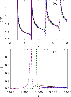
Figure 11: (color online) The total absorption probability $|D^{-}|^{2}$ (in arbitrary units) for a harmonic oscillator confining potential is plotted as a function of the scaled energy, $\epsilon=E/(\hbar\omega_{\perp})$. In panel (a) and (b) the lines are calculations using Eq. (50). The black solid line is the result when $\eta_{00}=0$. The red dotted and green dashed lines correspond to $a_{s}(E)/a_{\perp}=0.02$ and $-0.02$ respectively. The blue dash-dot and purple dot-dot-dash-dot lines are $a_{s}(E)/a_{\perp}=0.04$ and $-0.04$ respectively. Panel (b) consists of a magnification of panel (a) around the threshold energy $\epsilon=3$.

The result of photodetachment of an electron from a negative ion in a magnetic field was treated in Ref. Greene (1987) and is similar to the example of photodetachment in an isotropic, two-dimensional harmonic oscillator potential. However, in Ref. Greene (1987), only the effect of open channels is taken into account. This is equivalent to setting $\eta_{\ell m}(E)=0$ in Eq. (50) above. Thus, the results in Ref. Greene (1987) are an approximation to the full treatment which includes the effects of the closed channels. Since the formalism of Ref. Greene (1987) has been successfully applied in many circumstances, it is worth investigating the regimes where this approximation ($\eta_{\ell m}=0$) is adequate. Figure 11 depicts the total photoabsorption probability (in arbitrary units) for different $s$-wave scattering lengths that are a small fraction of $a_{\perp}$ which is the typical case for photodetachment in laboratory strength magnetic fields. The black solid line is the result from the approximation of Ref. Greene (1987). For small positive scattering length (see red dotted and blue dash-dot line in Fig.11(a)) , the photoabsorption cross section vanishes below and above each channel threshold whereas the black solid line vanishes only above every the threshold. Note that the cross section vanishes around every threshold also for negative scattering lengths [see green dashed and purple dot-dot dashed lines in Fig.11(a)]. Moreover, the case of negative scattering lengths exhibits another qualitative difference from the approximation of Ref. Greene (1987). More specifically, this can be seen in Fig.11(b) where the total photoabsorption probability for negative scattering length (green dashed and purple dot-dot-dashed lines) possesses a resonance barely below the channel threshold. This non-trivial resonant feature is absent from the black solid line manifesting in this manner the importance of the closed channel physics. In addition, Fig.11 (a) and (b) shows that away from the channel thresholds our results are practically the same as in the approximation of Ref. Greene (1987), [black solid line in Fig.11]. Note that there is one energy between each threshold where all of the results are the same. These are the energies where $\eta_{00}=0$.

Evidently, the role of the closed channels becomes important only around each threshold due to small scattering lengths. This explains why the result of Ref. Greene (1987) works well for photodetachment in a magnetic field. In this situation, the scattering length is of the order of a few Bohr radii while the confinement length is $a_{\perp}=a_{0}\sqrt{B_{a.u.}/B}$ where $a_{0}$ is the Bohr radius and $B_{a.u.}$ is the atomic unit of magnetic field. Thus, even in a 1 T magnetic field, the scattering length will typically be less than $a_{\perp}/100$. However, we expect that experiments would show differences from the treatment of Ref. Greene (1987) in stronger magnetic fields or for a negative ion whose photodetachment probes a final state having a much larger electron-atom scattering length.

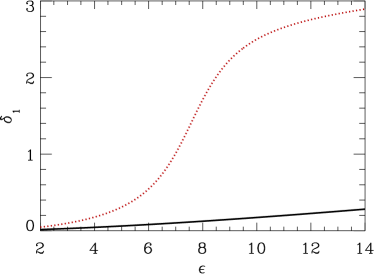
Figure 12: (color online) The $\ell=1$ phase shifts used in the calculations of Fig. 13. The black solid line is a non-resonance example and the red dotted line is the resonance case. The energy of the resonance is $\epsilon_{r}=7.8$.

The photodetachment for higher partial waves may possess shape resonances which allows for a larger effect from the closed channel collective state described by $\eta_{\ell m}(E)$. Therefore in the following, consider a photodetachment process into $\ell=1,m=1$ for a harmonic oscillator confinement. The confining potential does not have as strong an effect on the $\ell=1,m=0$ case because the outgoing flux is mostly along the $z$-axis compared to $m=1$ where the outgoing flux is mainly perpendicular to the $z$-axis. The energy dependent scattering volume is given by the relation $\tan\delta_{1}(E)/[ka_{\perp}]^{3}$ where a resonance form for the phase shift, $\delta_{1}$ is chosen according to the relation:

$$\tan\delta_{1}=-k^{3}\left[f_{sc}a_{\perp}^{3}+\frac{\gamma/k_{r}^{3}}{\epsilon-\epsilon_{r}}\right]$$ (80)

where $\epsilon=E/(\hbar\omega_{\perp})$ is the scaled energy with $E=\hbar^{2}k^{2}/2\mu$, $\epsilon_{r}=E_{r}/(\hbar\omega_{\perp})$ is the scaled energy of the resonance with $E_{r}=\hbar^{2}k_{r}^{2}/2\mu$, $\gamma$ is a parameter proportional to the scaled energy width of the resonance, and $f_{sc}$ is the scaled scattering volume. Figure 12 shows the $\delta_{1}$ phase shifts for a resonance case (red dotted line) with $f_{sc}=-(1/8)^{3}$, $\gamma=1.4$, and $\epsilon_{r}=7.8$ and for a non-resonance case (black solid line) $f_{sc}=-(1/8)^{3}$ and $\gamma=0$. For the energy dependent smooth dipole, $D_{s}(E)$, the following form is chosen

$$D_{s}(E)=k^{3/2}\left[d_{s}+(d_{r}/a_{\perp}^{3})\frac{\gamma/k_{r}^{3}}{\epsilon-\epsilon_{r}}\right]$$ (81)

where $d_{s}$ represents the amplitude for photoabsorption directly to the continuum and $d_{r}$ represents the amplitude for photoabsorption into the resonance. Figure 13 shows the results from 4 different calculations. In all calculations, the green dotted line is the photoabsorption that would occur if there were no confining potential, the black solid line corresponds to the full calculation with the confining potential, and the red dashed line is the approximation in Ref. Greene (1987) where the effect of the closed channels is neglected which is equivalent to setting $\eta_{11}=0$. As expected, the resonance features from the confinement calculations give an overall shape that tracks the non-confinement calculations, but with sharp features near the thresholds. The topmost calculations are when there is no resonance $\gamma=0$. The “Lorentz” calculation has $d_{s}=0$; it does not look like the standard Lorentzian shape resonance due to the overall increase proportional to $\epsilon^{3/2}$. The “Window” calculation has $d_{r}=0$; as with the Lorentz calculation, this does not look like the symmetrical window resonance due to the overall increase. The “Fano” calculation has $d_{r}/d_{s}=60$ which gives a 0 in the dipole matrix element at $\epsilon\simeq 9.1$ which is at a somewhat higher energy than the resonance position at 7.8. The full and approximate confinement calculations differ most strongly where $\tan\delta_{1}$ is large which is near the resonance and an energy range near the thresholds. For the three cases with the resonance at $\epsilon_{r}=7.8$, the absorption cross section shows sharp resonances below each threshold only for $\epsilon<\epsilon_{r}$ because the scattering volume is negative in this range.

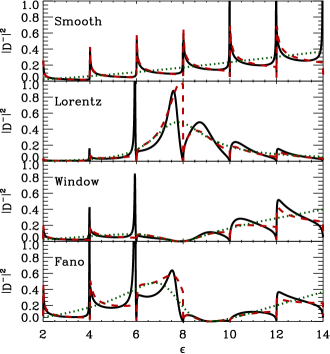
Figure 13: (color online) The $\ell=1$ photoabsorption $|D^{-}|^{2}$ (in arbitrary units) for different cases. In all calculations, the green dotted line is for photoabsorption with no confining potential, the red dashed line is the approximation that includes the confining potential but does not include the effect of closed channels (equivalent to setting $\eta_{11}=0$), and the black solid line is the full calculation including the confining potential. The “Smooth” calculation does not have a resonance. The “Lorentz”, “Window”, and “Fano” calculations only differ in the energy dependence of the dipole matrix element when no field is applied.

VII Summary and Conclusions

VII.1 Summary of Method

It is evident that there are many steps in the derivation and application of the Schwinger variational approach to collisions involving a short range spherically symmetric potential in the presence of various types of confining geometries. Therefore, in this section, the important steps are pointed out for applying the method. First, Eq. (43) gives the expression for the $K$-matrix and Eq. (46) gives the dipole matrix element in terms of the scattering length or volume and the energy dependent parameters $\mathcal{U}_{\alpha,\ell m}$ and $\eta_{\ell m}$. The conversion from spherical coordinates to the confinement geometry is encapsulated in the $\mathcal{U}_{\alpha,\ell m}$ in Eq. (44) which depends on the confinement wave functions $\Phi_{\alpha}(x,y)$ at the scatterer.

In this paper, the expressions for the $\eta_{\ell m}$ were obtained from a detailed examination of the confinement Green’s function, $\hat{G}_{c}$, and various integral expressions for the free Green’s function, $\hat{G}_{f}$. There is a conceptual shortcut that can be used to obtain the $\eta_{\ell m}$: the $\hat{G}_{c}$ becomes the $\hat{G}_{f}$ in the limit that the confinement length scale, $a_{\perp}$, goes to infinity. This is the reason that the $\eta_{\ell m}$ have the form of a sum (from the $\hat{G}_{c}$) minus an integral that has the same functional form (from the $\hat{G}_{f}$ as formulated from $\hat{G}_{c}$ in the limit $a_{\perp}\to\infty$). Similar to Eq. (44), define a transformation for the closed channels

$$\bar{\mathcal{U}}_{\alpha,\ell m}=\begin{cases}\sqrt{\frac{2\pi}{\tilde{\kappa}_{\alpha}}}a_{\perp}\Phi_{\alpha}(\bm{\rho}_{s})&\ell=m=0\\ \sqrt{6\pi\tilde{\kappa}_{\alpha}}a_{\perp}\Phi_{\alpha}(\bm{\rho}_{s})&\ell=1,\leavevmode\nobreak\ m=0\\ -\sqrt{\frac{12\pi}{\tilde{\kappa}_{\alpha}}}a_{\perp}^{2}(\partial_{\pm}\Phi_{\alpha})\big{|}_{\bm{\rho}_{s}}&\ell=1,\leavevmode\nobreak\ m=\pm 1\end{cases}$$ (82)

where the operators are defined below Eq. (33), $\bm{\rho}_{s}$ is the position of the scatterer, and $E=-\hbar^{2}\tilde{\kappa}^{2}_{\alpha}/(2\mu a_{\perp}^{2})+E_{\alpha}$. Since $\Phi_{\alpha}$ is proportional to $1/a_{\perp}$, the $\bar{\mathcal{U}}$ only depends on the form of the confining potential, the scaled energy, and the $\bm{\rho}_{s}/a_{\perp}$. In this paper, we restricted the confining potential to be independent of $z$ and symmetric in $xy$. For these cases, the following relation between $\eta$ and $\bar{\mathcal{U}}$ hold

$$\eta_{\ell m}=(-1)^{\ell+m} [\sum_{\alpha>\alpha_{o}}^{\infty}|\bar{\mathcal{U}}_{\alpha,\ell m}|^{2}e^{-\tilde{\kappa}_{\alpha}\Delta\tilde{z}}$$ (83)

$$- \int_{\alpha\geq\alpha_{o}}^{\infty}|\bar{\mathcal{U}}_{\alpha,\ell m}|^{2}e^{-\tilde{\kappa}_{\alpha}\Delta\tilde{z}}d\alpha]$$ (84)

where the limit $\Delta\tilde{z}\to 0^{+}$ is understood. The integral over $d\alpha$ is the result of the quantum numbers for $G_{f}$ giving an infinitesimal spacing of $\kappa_{\alpha}$ in the limit $a_{\perp}\to\infty$. For the case of Sec. VI.1.3 which does not satisfy the restrictions on the confining potential, the $|\bar{\mathcal{U}}_{\alpha,\ell m}|^{2}$ is replaced with the average value as $a_{\perp}\to\infty$.

VII.2 Conclusions

In the preceding sections, the development of a Schwinger variational framework is presented as a treatment of scattering in a confined geometry. The current formalism is non-perturbative, permitting the treatment of a wide class of Hamiltonian systems which possess two potentials. The particular type of Hamiltonians studied in this work consists of systems where the interaction at short distances is spherically symmetric and, at large distances, a confining potential is considered which bounds the motion of the particle in the degrees of freedom perpendicular to the direction of its propagation. The restriction in the current formalism amounts to the fact that the considered potentials dominate at different scales. For the sake of simplicity, we restricted the confining potential to have no dependence in the $z$-coordinate and symmetry in $xy$. However, this theoretical method could treat general confining potentials where length scale separation holds.

The theoretical formalism presented in this paper allows a self-consistent treatment of scattering in a confined geometry where the results are manifestly convergent at each step of the derivation. This formalism has been used to derive results obtained in previous studies (e.g. s- and p-wave scattering within a harmonic confining potential and s-wave scattering in a square well confining potential) and to quickly derive results in novel geometries (e.g. s-wave and p-wave scattering in off-center confining potentials and scattering in rectangular confining potentials). Results for the scattering parameters in different geometries were presented and main qualitative features were explained. The formalism was also used to derive a treatment of half-scattering problems (e.g. photo-detachment) in confining potentials. For example, the photo-detachment results in a harmonic confinement was compared to a previous LFT treatment that only accounted for open channels to assess the role of the closed channels which are included in this treatment: the effect from the closed channels are most important near thresholds and become more important as the scattering length becomes a sizable fraction of the confinement length scale.

An interesting possibility for the formalism in this paper is to aid in the understanding of the implementation and possible limitations of the LFT. The basic steps in the current formalism were cast in a form strongly reminiscent of the LFT. However, these two frameworks possess a conceptual difference which is mainly focused on the physics of the closed channels. More specifically, in the LFT approach the $K$-matrix formulas include diverging sums and therefore regularization schemes are employed to remove such singularities. In the Schwinger variational approach, such divergences do not emerge, which eliminates the need for tricky regularization techniques that are often used in the LFT theory. In particular, we observe that in the physical $K$-matrix of the LFT the information of the free space $\hat{G}_{f}$ is absent and it has been indirectly incorporated via regularization schemes Granger and Blume (2004); Giannakeas et al. (2012); Zhang and Greene (2013).

In view of the rigorousness of the Schwinger variational approach, we expect that it can be equally applied to other physical systems where the LFT method has been used. For example, this method can be used to derive the scattering of an electron in a Rydberg state from a neutral perturber and, for $\ell=0$, the same result as Eq. (14) of Ref. Du and Greene (1987) is obtained. Note that the frame transformation ideas have been used in many different circumstances. A short list of examples could include the $jj-LS$ transformation, molecular rotational transformations, molecular vibrational transformations, local frame transformations involving external electric and/or magnetic fields. In all cases, wave functions in one representation are projected on those in another representation at a surface (or indirectly in a region) where both representations are expected to be accurate. However, the level of error involved in such a procedure is not clear. It is conceivable that the method described above might enable a more systematic derivation of the frame transformation so that the level of expected error would be clearer.

Appendix A Matrix elements with $\hat{V}_{s}\ket{\psi_{s}}$

The volume integral in Eq. (30) can be simplified by employing the relation $\hat{V}_{s}\ket{\psi_{s}}=(E-\hat{H}_{f})\ket{\psi_{s}}$. Then, assuming length scale separation, the confining potential $\hat{V}_{c}$ is practically zero in the range of $\hat{V}_{s}$ where the following relation is valid $(E-\hat{H}_{c})\ket{\psi_{c}}\approx(E-\hat{H}_{f})\ket{\psi_{c}}\approx 0$. Thus, integrating by parts twice Eq. (30), the terms of $(E-\hat{H}_{f})\ket{\psi_{c}}$ vanish and only the surface ones survive. In general, the following relation is fulfilled:

$$\braket{\psi_{c}}{\hat{V}_{s}}{\psi_{s}}=\frac{\hbar^{2}}{2\mu}\int_{\sigma(\tau)}\hat{n}\cdot\{\psi_{c}^{*}(\mathbf{r})[\vec{\nabla}\psi_{s}(\mathbf{r})]-[\vec{\nabla}\psi_{c}^{*}(\mathbf{r})]\psi_{s}(\mathbf{r})\}d\sigma$$ (85)

where $\sigma(\tau)$ indicates the surface containing the volume $\tau$ and $\hat{n}$ is the unit vector which is outward normal to the surface. If the region $\tau$ is a sphere of radius $r$, this matrix element can be written as

$$\braket{\psi_{c}}{\hat{V}_{s}}{\psi_{s}}=\frac{\hbar^{2}}{2\mu}r^{2}\int\bigg{[}\psi_{c}^{*}(\mathbf{r})\frac{\partial\psi_{s}(\mathbf{r})}{\partial r}-\frac{\partial\psi_{c}^{*}(\mathbf{r})}{\partial r}\psi_{s}(\mathbf{r})\bigg{]}d\Omega$$ (86)

where $d\Omega=\sin\theta d\theta d\phi$ is the solid angle differential element.

This subsection recast the integrals which involve $\hat{V}_{s}\ket{\psi_{s}}$ into surface integrals when length scale separation between $\hat{V}_{s}$ and $\hat{V}_{c}$ is a good approximation. The following subsections focus on special cases where $\ket{\psi_{s}}$ is an eigenstate of angular momentum $\ell$ and its projection, providing explicit analytical equations for this situation.

A.1 Analytic expressions of $\braket{\psi_{c}}{\hat{V}_{s}}{\psi_{s}}$ for $\ell=0,\leavevmode\nobreak\ m=0$

Assume that in this case study the states $\ket{\psi_{s}}\equiv\ket{\psi_{s,\ell m}}$ possess $\ell=0,\leavevmode\nobreak\ m=0$ character. At distances where the $\hat{V}_{c}$ potential is considered small, the $\psi_{c}(\mathbf{r})$ to a good approximation can be written as a linear combination of spherical Bessel functions times spherical harmonics, $j_{\ell}(kr)Y_{\ell m}(\Omega)$. Note that the wave number $k$ corresponds to the total energy and $\Omega$ denotes the $(\theta,\leavevmode\nobreak\ \phi)$-angles. The coefficients of the linear combination can be specified by expanding in Taylor series the $\psi_{c}(\mathbf{r})$ and $j_{\ell}(kr)Y_{\ell m}(\Omega)$ functions and matching them term by term. However, at small distances only few terms are needed to be matched.

The coefficient of the $j_{0}(kr)Y_{00}(\Omega)$ term is simply $\sqrt{4\pi}$ times the value of $\psi_{c}(\mathbf{r})$ at the origin giving

$$\psi_{c}(\mathbf{r})\simeq\psi_{c}(0)\sqrt{4\pi}j_{0}(kr)Y_{00}(\Omega)$$ (87)

After substituting this expression into Eq. (86) the surface integral yields the following general form:

$$\braket{\psi_{c}}{\hat{V}_{s}}{\psi_{s}}=\sqrt{\frac{\pi\hbar^{2}}{\mu}}\psi_{c}(0)\sqrt{\frac{2\pi}{k}}\left(-\frac{1}{\pi}\tan\delta_{0}\right),$$ (88)

where the expressions have been used for the $\psi_{c}(\mathbf{r})\equiv\psi^{(e)}_{c,\alpha}(\mathbf{r})$ [see Eq. (6)] and $\psi_{s}(\mathbf{r})\equiv\psi_{s,00}(\mathbf{r})$ Eq. (88) reads

$$\braket{\psi^{(e)}_{c,\alpha}}{\hat{V}_{s}}{\psi_{s,00}}=\Phi^{*}_{\alpha}(0,0)\sqrt{\frac{2\pi}{kk_{\alpha}}}\left(-\frac{1}{\pi}\tan\delta_{0}\right)$$ (89)

A.2 Analytic expressions of $\braket{\psi_{c}}{\hat{V}_{s}}{\psi_{s}}$ for $\ell=1,\leavevmode\nobreak\ m=0$

This subsection focuses on the case where $\ket{\psi_{s}}\equiv\ket{\psi_{s,\ell m}}$ possesses an $\ell=1,\leavevmode\nobreak\ m=0$ character. In a similar way as was discussed in the previous subsection the $\psi_{c}(\mathbf{r})$ functions are matched to the superposition of spherical Bessel functions times spherical harmonics, $j_{\ell}(kr)Y_{\ell m}(\Omega)$. In this particular case the coefficient of the $j_{1}(kr)Y_{10}$ term is simply $\sqrt{12\pi}/k$ times the value of $\partial\psi_{c}(\mathbf{r})/\partial z$ at the origin.

$$\psi_{c}(\mathbf{r})\simeq\frac{\partial\psi_{c}(\mathbf{r})}{\partial z}\Bigg{|}_{|\mathbf{r}|=0}\frac{\sqrt{12\pi}}{k}j_{1}(kr)Y_{10}(\Omega)$$ (90)

Substituting this expression into Eq. (86) the surface integral reads:

$$\braket{\psi_{c}}{\hat{V}_{s}}{\psi_{s}}=\sqrt{\frac{\pi\hbar^{2}}{\mu}}\frac{\partial\psi_{c}(\mathbf{r})}{\partial z}\Bigg{|}_{|\mathbf{r}|=0}\sqrt{\frac{6\pi}{k^{3}}}\left(-\frac{1}{\pi}\tan\delta_{1}\right),$$ (91)

where using the expressions for the $\psi_{c}(\mathbf{r})\equiv\psi^{(o)}_{c,\alpha}(\mathbf{r})$ from Eq. (6) and $\psi_{s}(\mathbf{r})\equiv\psi_{s,10}(\mathbf{r})$ Eq. (91) reads

$$\braket{\psi^{(o)}_{c,\alpha}}{\hat{V}_{s}}{\psi_{s,10}}=\Phi^{*}_{\alpha}(0,0)\sqrt{\frac{6\pi k_{\alpha}}{k^{3}}}\left(-\frac{1}{\pi}\tan\delta_{1}\right)$$ (92)

A.3 Analytic expressions of $\braket{\psi_{c}}{\hat{V}_{s}}{\psi_{s}}$ for $\ell=1,\leavevmode\nobreak\ m=\pm 1$

This subsection considers the case where $\ket{\psi_{s}}\equiv\ket{\psi_{s,\ell m}}$ possesses $\ell=1,\leavevmode\nobreak\ m=\pm 1$ character. Therefore in this case the coefficient of the $j_{1}(kr)Y_{1\pm 1}(\Omega)$ term is simply $-\sqrt{24\pi}/k$ times the value of $(\partial\psi_{c}(\mathbf{r})/\partial x\mp i\partial\psi_{c}(\mathbf{r})/\partial y)/2$ at the origin yielding the following relation:

$$\psi_{c}(\mathbf{r})\simeq-(\partial_{\pm}\psi_{c})\Bigg{|}_{|\mathbf{r}|=0}\frac{\sqrt{24\pi}}{k}j_{1}(kr)Y_{1\pm 1}(\Omega)$$ (93)

where $(\partial_{\pm}\psi_{c})\equiv(\partial\psi_{c}(\mathbf{r})/\partial x\mp i\partial\psi_{c}(\mathbf{r})/\partial y)/2$.

Substituting these expressions into the surface integral gives the simple result:

$$\braket{\psi_{c}}{\hat{V}_{s}}{\psi_{s}}=\sqrt{\frac{\pi\hbar^{2}}{\mu}}(\partial_{\pm}\psi_{c})^{*}\Bigg{|}_{0}\sqrt{\frac{12\pi}{k^{3}}}\left(-\frac{1}{\pi}\tan\delta_{1}\right),$$ (94)

where using the expressions for the $\psi_{c}(\mathbf{r})\equiv\psi^{(e)}_{c,\alpha}(\mathbf{r})$ from Eq. (6) and $\psi_{s}(\mathbf{r})\equiv\psi_{s,1\pm 1}(\mathbf{r})$ Eq. (94) reads

$$\braket{\psi^{(e)}_{c,\alpha}}{\hat{V}_{s}}{\psi_{s,1\pm 1}}=-(\partial_{\pm}\Phi_{\alpha})^{*}\Bigg{|}_{0}\sqrt{\frac{12\pi}{k_{\alpha}k^{3}}}\left(-\frac{1}{\pi}\tan\delta_{1}\right)$$ (95)

Appendix B Evaluation of the $D_{s}$ matrix elements

At this point, all of the terms in the expression for the $K$-matrix, Eq. (26) have a simple analytic expression except for the term involving the matrix element of $\hat{V}_{s}\Delta\hat{G}\hat{V}_{s}$, see Eq. (29). The most straightforward method for evaluating this matrix element is to individually compute the matrix elements of $\hat{V}_{s}\hat{G}_{f}\hat{V}_{s}$ and $\hat{V}_{s}\hat{G}_{c}\hat{V}_{s}$ and subtract. However, this method is fraught with difficulties because each of these matrix elements involve integrands that diverge.

At the symmetry point of $\hat{V}_{c}$, the function $\Delta\hat{G}$ only has even powers of $(z_{1}-z_{2})$ and powers of $\bm{\rho}_{1}\cdot\bm{\rho}_{2}$ through second order if the confining potential is a power series in $x,y,z$. The vector $\bm{\rho}_{1}\equiv\hat{x}x_{1}+\hat{y}y_{1}$. Thus, the matrix element in Eq. (29) only has terms from regular functions at least to order $r^{3}$. If the state $\ket{\psi_{s}}$ possesses $\ell=0$ or $\ell=1,\leavevmode\nobreak\ m$ character, then only terms in $\Delta\hat{G}$ proportional to $(z_{1}-z_{2})^{0}$, $(z_{1}-z_{2})^{2}$, and $(\bm{\rho}_{1}-\bm{\rho}_{2})^{2}$ will contribute to the integral:

$$\Delta G(\mathbf{r}_{1},\mathbf{r}_{2})\simeq\Delta G(0)-\Delta G_{zz}(0)z_{1}z_{2}-\Delta G_{\rho\rho}(0)\bm{\rho}_{1}\cdot\bm{\rho}_{2},$$ (96)

where $\Delta G(0)$, $\Delta G_{zz}$ and $\Delta G_{\rho\rho}$ are coefficients that will be determined below. Note that terms proportional to $x_{j}^{2}$, $y_{j}^{2}$, and $z_{j}^{2}$ are not included since they only affect matrix elements for $d$-wave scattering or give small corrections to the $s$-wave scattering. Recall that $\Delta\hat{G}$ is a real function since its constituents (i.e. $\hat{G}_{f}$ and $\hat{G}_{c}$) are the principal value Green’s functions. Using this expansion, the dominant contribution to the $D_{s}$ matrix element for the $\ell=0,\leavevmode\nobreak\ m=0$ case is the $\Delta G(0)$ term

$$D_{s,00} = \braket{\psi_{s,00}}{\hat{V}_{s}}{z_{1}^{0}}\Delta G(0)\braket{z_{2}^{0}}{\hat{V}_{s}}{\psi_{s,00}}$$ (97)

$$= \Delta G(0)\frac{\pi\hbar^{2}}{\mu}\frac{2\pi}{k}\left(-\frac{1}{\pi}\tan\delta_{0}\right)^{2}$$ (98)

For the case of $\ell=1,\leavevmode\nobreak\ m=0$ the dominant contribution to the $D_{s}$ matrix elements is from the term $-z_{1}z_{2}\Delta G_{zz}(0)$

$$D_{s,10} = -\braket{\psi_{s,10}}{\hat{V}_{s}}{z_{1}}\Delta G_{zz}(0)\braket{z_{2}}{\hat{V}_{s}}{\psi_{s,10}}$$ (99)

$$= -\Delta G_{zz}(0)\frac{\pi\hbar^{2}}{\mu}\frac{6\pi}{k^{3}}\left(-\frac{1}{\pi}\tan\delta_{1}\right)^{2}$$ (100)

Similarly, for the case of $\ell=1,m=\pm 1$ the dominant contribution to the $D_{s}$ matrix elements emerges from the term $-\bm{\rho}_{1}\cdot\bm{\rho}_{2}\Delta G_{\rho\rho}(0)$

$$D_{s,1\pm 1} = -\braket{\psi_{s,1\pm 1}}{\hat{V}_{s}}{\rho_{1}e^{\pm i\phi_{1}}}\Delta\hat{G}_{\rho\rho}(0)\braket{\rho_{2}e^{\pm i\phi_{2}}}{\hat{V}_{s}}{\psi_{s,1\pm 1}}$$ (101)

$$= -\Delta G_{\rho\rho}(0)\frac{\pi\hbar^{2}}{\mu}\frac{6\pi}{k^{3}}\left(-\frac{1}{\pi}\tan\delta_{1}\right)^{2}$$ (102)

Appendix C $\eta_{\ell m}(E)$ functions for given confining geometries

In the expressions for the Green’s functions, we only need terms through $\bm{\rho}_{1}\cdot\bm{\rho}_{2}$. The free space Green’s function, $\hat{G}_{f}$ is Taylor expanded up to terms proportional to $\bm{\rho}_{1}\cdot\bm{\rho}_{2}$ which give

$$\frac{\cos(\tilde{k}\tilde{r}_{12})}{|\tilde{r}_{12}|}\simeq\frac{\cos(\tilde{k}\Delta\tilde{z})}{|\Delta\tilde{z}|}+\frac{\bm{\rho}_{1}\cdot\bm{\rho}_{2}}{a_{\perp}^{2}}\left(\frac{\cos(\tilde{k}\Delta\tilde{z})}{|\Delta\tilde{z}|^{3}}+\frac{\tilde{k}\sin(\tilde{k}\Delta\tilde{z})}{\Delta\tilde{z}^{2}}\right)$$ (103)

where the scaled variables are $\tilde{k}=ka_{\perp}$ and $\Delta\tilde{z}=\Delta z/a_{\perp}$. The strategy below will be to write this expression for $\hat{G}_{f}$ as an integral with a uniformly converging integrand. We will show that this integral will be the continuum form of the sums that arise in $\hat{G}_{c}$.

In this subsection, the functions $\eta_{\ell m}(E)$ are derived for two types of confining potentials, i.e. harmonic and infinitely square well confining potential. In addition, we compare the approximation Eq. (41) to the full expression for $\Gamma(E)$ as a function of $\Delta\tilde{z}$, Eq. (38) as an illustration of the accuracy of the $\eta_{\ell m}(E)$.

C.1 Harmonic Oscillator Confining Potential

In this section, the motion of the particle in the transversal degrees of freedom is bounded by a harmonic oscillator which possesses the form $V_{c}(\rho)=\frac{\mu}{2}\omega_{\perp}\rho^{2}$ where $\mu$ denotes the mass of the particle, $\omega_{\perp}$ corresponds to the frequency of the harmonic confinement corresponding to the length scale $a_{\perp}=\sqrt{\hbar/\mu\omega_{\perp}}$. Note that the variable $\rho$ represents the polar coordinate, namely $\rho=\sqrt{x^{2}+y^{2}}$.

Under these considerations, the motion of the photoelectron separates in the $z,\leavevmode\nobreak\ \rho$ degrees of freedom. The solutions of the corresponding Hamiltonian, namely $\hat{H}_{c}$, possess the form given in Eq. (6) for even or odd parity in $z$-direction. Accordingly, the eigenenergies of the Hamiltonian $\hat{H}_{c}$ fulfill the relation $E=\hbar\omega_{\perp}(2n+|m|+1)+\hbar^{2}k^{2}_{n,|m|}/(2\mu)$, where $n=0,1,\ldots$. Evaluating the harmonic oscillator eigensolutions at the $(\rho,\leavevmode\nobreak\ \phi)\to 0$ the following relations are obtained

$$\begin{cases}\Phi_{n,m}(0)=\frac{1}{a_{\perp}\sqrt{\pi}}&\rm{for}\leavevmode\nobreak\ m=0\\ (\partial_{\pm}\Phi_{n,m})(0)=\frac{\sqrt{n+1}}{a^{2}_{\perp}\sqrt{\pi}}&\rm{for}\leavevmode\nobreak\ m=\pm 1\end{cases}$$ (104)

The scaled energy is defined by the relation $\epsilon=E/(\hbar\omega_{\perp})$. The scaled momenta can be written as $\tilde{k}=\sqrt{2\epsilon}$, $\tilde{k}_{nm}=\sqrt{2\epsilon-2(2n+|m|+1)}$, and $\tilde{\kappa}_{nm}=\sqrt{2(2n+|m|+1)-2\epsilon}$. Substituting Eq. (104) in Eq. (38) with the approximation of Eq. (103), the following relation is obtained

$$\Gamma(\bm{r}_{1},\bm{r}_{2},E)= - 2\sum_{n=0}^{n_{o,0}}\frac{\sin(\tilde{k}_{n0}\Delta\tilde{z})}{\tilde{k}_{n0}}+2\sum_{n=n_{o,0}+1}^{\infty}\frac{e^{-\tilde{\kappa}_{n0}\Delta\tilde{z}}}{\tilde{\kappa}_{n0}}$$ (105)

$$+ 2\int_{-1/2}^{n_{o,0}}\frac{\sin(\tilde{k}_{n0}\Delta\tilde{z})}{\tilde{k}_{n0}}dn-2\int_{n_{o,0}}^{\infty}\frac{e^{-\tilde{\kappa}_{n0}\Delta\tilde{z}}}{\tilde{\kappa}_{n0}}dn$$ (106)

$$- \tilde{\bm{\rho}}_{1}\cdot\tilde{\bm{\rho}}_{2}4\sum_{n=0}^{n_{o,1}}\frac{(n+1)\sin(\tilde{k}_{n1}\Delta\tilde{z})}{\tilde{k}_{n1}}$$ (107)

$$+ \tilde{\bm{\rho}}_{1}\cdot\tilde{\bm{\rho}}_{2}4\int_{-1}^{n_{o,1}}\frac{(n+1)\sin(\tilde{k}_{n1}\Delta\tilde{z})}{\tilde{k}_{n1}}dn$$ (108)

$$+ \tilde{\bm{\rho}}_{1}\cdot\tilde{\bm{\rho}}_{2}4\sum_{n=n_{o,1}+1}^{\infty}\frac{(n+1)e^{-\tilde{\kappa}_{n1}\Delta\tilde{z}}}{\tilde{\kappa}_{n1}}$$ (109)

$$- \tilde{\bm{\rho}}_{1}\cdot\tilde{\bm{\rho}}_{2}4\int_{n_{o,1}}^{\infty}\frac{(n+1)e^{-\tilde{\kappa}_{n1}\Delta\tilde{z}}}{\tilde{\kappa}_{n1}}dn$$ (110)

where $n_{o,m}=(\epsilon-1-|m|)/2$ is the divide between open and closed channels; in the sums, the integer part should be used. Note that $\tilde{\bm{\rho}}_{1}\cdot\tilde{\bm{\rho}}_{2}=\bm{\rho}_{1}\cdot\bm{\rho}_{2}/a_{\perp}^{2}$. This expression has many terms but each can be identified with different parts of the Eq. (38). The first line is the contribution from the $m=0$ open (first term) and closed (second term) channels from $G_{c}$. The second line is an integral expression that exactly equals $-\cos(\tilde{k}\Delta\tilde{z})/\Delta\tilde{z}$ (see Eq. (103)) which is the contribution to $m=0$ from $\hat{G}_{f}$. The third (fifth) line is the contribution to $m=\pm 1$ from the open (closed) channels in $\hat{G}_{c}$. The fourth and sixth lines are an integral expression whose sum exactly equals the term in Eq. (103) multiplying the $\tilde{\bm{\rho}}_{1}\cdot\tilde{\bm{\rho}}_{2}$.

There are important features of Eq. (105) that affect how the scattering information is extracted. For example, the sums and integrals that correspond to the open channels all contain $\sin(\tilde{k}_{\alpha}\Delta\tilde{z})$ and therefore they do not contribute to $\Gamma$ as $\Delta\tilde{z}\to 0^{+}$ for $\Delta\rho\ll 1$. Terms which refer to the closed channels do survive in this limit and they contribute to the $\eta_{\ell m}(E)$. Lines 4 and 6 contribute to the $\eta_{1\pm 1}$ while the second term in each of lines 1 and 2 contribute to the $\eta_{00}$ and $\eta_{10}$. The $\eta_{00}$ is the limit as all spatial coordinates of $\Gamma$ go to 0. The $\eta_{10}=-3\partial^{2}\Gamma/\partial(\Delta\tilde{z})^{2}$ in the limit all spatial coordinates go to 0. This gives

$$\eta_{00} = 2\sum_{n=n_{o,0}+1}^{\infty}\frac{e^{-\tilde{\kappa}_{n0}\Delta\tilde{z}}}{\tilde{\kappa}_{n0}}-2\int_{n_{o,0}}^{\infty}\frac{e^{-\tilde{\kappa}_{n0}\Delta\tilde{z}}}{\tilde{\kappa}_{n0}}dn$$ (111)

$$\eta_{10} = -6\sum_{n=n_{o,0}+1}^{\infty}\tilde{\kappa}_{n0}e^{-\tilde{\kappa}_{n0}\Delta\tilde{z}}+6\int_{n_{o,0}}^{\infty}\tilde{\kappa}_{n0}e^{-\tilde{\kappa}_{n0}\Delta\tilde{z}}dn$$ (112)

$$\eta_{1\pm 1} = 12\sum_{n=n_{o,1}+1}^{\infty}\frac{(n+1)e^{-\tilde{\kappa}_{n1}\Delta\tilde{z}}}{\tilde{\kappa}_{n1}}$$ (114)

$$-12\int_{n_{o,1}}^{\infty}\frac{(n+1)e^{-\tilde{\kappa}_{n1}\Delta\tilde{z}}}{\tilde{\kappa}_{n1}}dn$$

where the limit $\Delta\tilde{z}\to 0^{+}$ is understood for all expressions. Notice that all of the terms have the form of a sum minus a corresponding integral. This feature ensures that the $\eta_{\ell m}$ are well defined for any finite $\Delta\tilde{z}$ and thus they give unambiguous, finite results in the limit $\Delta\tilde{z}\to 0^{+}$.

To summarize, the expressions needed for the calculation of the $K$-matrix are convergent series when using a finite $\Delta\tilde{z}$ in the expression for the Green’s function. When the scattering potential has a short range, analytic expressions can be obtained in the limit $\Delta\tilde{z}\to 0^{+}$.

C.2 Infinite Square Well Confinement

In this section, the motion of the particle is bounded in the $x$- and $y$-direction by an infinitely square well. The square well possesses the following form $V(x,y)=0$ when $|x|<a_{\perp}/2$ and $|y|<a_{\perp}/2$ and $V(x,y)=\infty$ elsewhere. As in the case of the harmonic oscillator at large distances the wave function of the electron separates in Cartesian coordinates, where the corresponding solutions of the Hamiltonian $\hat{H}_{c}$ possess the form in Eq. (6) for even or odd parity in the $z$-direction, respectively. In addition, the energy spectrum of the $\hat{H}_{c}$ Hamiltonian obeys the following relation $E=E_{n_{x},n_{y}}+\hbar^{2}k^{2}_{n_{x},n_{y}}/(2\mu)$ where $E_{n_{x}n_{y}}=\frac{\hbar^{2}\pi^{2}}{2\mu a_{\perp}^{2}}[n_{x}^{2}+n_{y}^{2}]$. For the $m=0$ case, we are only interested in the values of the quantum numbers $n$ that give non-zero functions at the origin; these correspond to the cases $n_{x},n_{y}=(2\alpha_{x}+1),(2\alpha_{y}+1)$ where the $\alpha_{x},\alpha_{y}$ are independently $0,1,2,...$. For the $m=1$ case, we use the functions

$$\Phi^{\pm}_{n_{x}n_{y}}(x,y)=\frac{1}{\sqrt{2}}[F_{n_{x}}(x)F_{n_{y}}(y)\pm iF_{n_{x}}(y)F_{n_{y}}(x)]$$ (115)

where $F_{n}(x)=\sqrt{2/a_{\perp}}\sin(n\pi[\tilde{x}-1/2])$ with $\tilde{x}=x/a_{\perp}$ and $n_{x},n_{y}=(2\alpha_{x}+2),(2\alpha_{y}+1)$ with the $\alpha_{x},\alpha_{y}$ independently $0,1,2,...$. This choice gives $F^{\prime}_{n_{x}}(0)\neq 0$ and $F_{n_{y}}(0)\neq 0$. This particular linear combination in Eq. (115) ensures that collisions with $m=1$ affect the square well states whose $x$-dependent factor vanishes at the origin while the $y$-dependent factor is nonzero, or vice versa. Evaluation of the square well eigensolutions at the origin gives

$$\begin{cases}\Phi_{\alpha_{x}\alpha_{y}}(0,0)=\frac{2(-1)^{\alpha_{x}+\alpha_{y}}}{a_{\perp}}\leavevmode\nobreak\ \leavevmode\nobreak\ {\rm{for}}\leavevmode\nobreak\ m=0\\ (\partial_{\pm}\Phi^{\pm}_{\alpha_{x}\alpha_{y}})\big{|}_{0}=\frac{\sqrt{2}(-1)^{\alpha_{x}+\alpha_{y}+1}}{a_{\perp}}\frac{2\pi(\alpha_{x}+1)}{a_{\perp}}\leavevmode\nobreak\ \leavevmode\nobreak\ {\rm{for}}\leavevmode\nobreak\ m=1,\end{cases}$$ (116)

where the functions $\Phi^{\pm}_{n_{x}n_{y}}(x,y)$ are defined in Eq. (115)

We define the scaled energy to be $\epsilon=E/(4\hbar^{2}\pi^{2}/[2\mu a_{\perp}^{2}])$. The scaled momenta can be written as $\tilde{k}=2\pi\sqrt{\epsilon}$, $\tilde{k}_{\alpha m}=2\pi\sqrt{\epsilon-[(\alpha_{x}+[|m|+1]/2)^{2}+(\alpha_{y}+1/2)^{2}]}$, and $\tilde{\kappa}_{\alpha m}=2\pi\sqrt{(\alpha_{x}+[|m|+1]/2)^{2}+(\alpha_{y}+1/2)^{2}-\epsilon}$. Substituting Eq. (116) in Eq. (38) the following relation is obtained:

$$\Gamma(\bm{r}_{1},\bm{r}_{2},E)= - 8\pi\sum_{\alpha=0}^{\alpha_{o,0}}\frac{\sin(\tilde{k}_{\alpha 0}\Delta\tilde{z})}{\tilde{k}_{\alpha 0}}+8\pi\sum_{\alpha=\alpha_{o,0}+1}^{\infty}\frac{e^{-\tilde{\kappa}_{\alpha 0}\Delta\tilde{z}}}{\tilde{\kappa}_{\alpha 0}}$$ (117)

$$+ 8\pi\int_{-1/2}^{\alpha_{o,0}}\frac{\sin(\tilde{k}_{\alpha 0}\Delta\tilde{z})}{\tilde{k}_{\alpha 0}}d^{2}\alpha-8\pi\int_{\alpha_{o,0}}^{\infty}\frac{e^{-\tilde{\kappa}_{\alpha 0}\Delta\tilde{z}}}{\tilde{\kappa}_{\alpha 0}}d^{2}\alpha$$ (118)

$$- \tilde{\bm{\rho}}_{1}\cdot\tilde{\bm{\rho}}_{2}32\pi^{3}\sum_{\alpha=0}^{\alpha_{o,1}}\frac{(\alpha_{x}+1)^{2}\sin(\tilde{k}_{\alpha 1}\Delta\tilde{z})}{\tilde{k}_{\alpha 1}}$$ (119)

$$+ \tilde{\bm{\rho}}_{1}\cdot\tilde{\bm{\rho}}_{2}32\pi^{3}\int_{-1}^{\alpha_{o,1}}\frac{(\alpha_{x}+1)^{2}\sin(\tilde{k}_{\alpha 1}\Delta\tilde{z})}{\tilde{k}_{\alpha 1}}d^{2}\alpha$$ (120)

$$+ \tilde{\bm{\rho}}_{1}\cdot\tilde{\bm{\rho}}_{2}32\pi^{3}\sum_{\alpha=\alpha_{o,1}+1}^{\infty}\frac{(\alpha_{x}+1)^{2}e^{-\tilde{\kappa}_{\alpha 1}\Delta\tilde{z}}}{\tilde{\kappa}_{\alpha 1}}$$ (121)

$$- \tilde{\bm{\rho}}_{1}\cdot\tilde{\bm{\rho}}_{2}32\pi^{3}\int_{\alpha_{o,1}}^{\infty}\frac{(\alpha_{x}+1)^{2}e^{-\tilde{\kappa}_{\alpha 1}\Delta\tilde{z}}}{\tilde{\kappa}_{\alpha 1}}d^{2}\alpha$$ (122)

where $\alpha_{o,m}$ denotes the divide between open and closed channels and is given by $(\alpha_{x}+[|m|+1]/2)^{2}+(\alpha_{y}+1/2)^{2}=\epsilon$; in the sums, the integer part of $\alpha_{x},\alpha_{y}$ should be used. Note that $\tilde{\bm{\rho}}_{1}\cdot\tilde{\bm{\rho}}_{2}=\bm{\rho}_{1}\cdot\bm{\rho}_{2}/a_{\perp}^{2}$. This expression has many terms but each can be identified with different parts of the Eq. (38). The first line is the contribution from the $m=0$ open (first term) and closed (second term) channels from $\hat{G}_{c}$. The second line is an integral expression that exactly equals $-\cos(\tilde{k}\Delta\tilde{z})/\Delta\tilde{z}$ (see Eq. (103)) which is the contribution to $m=0$ from $G_{f}$; the lower limit of integration is $-1/2$ for both $\alpha_{x}$ and $\alpha_{y}$. The third (fifth) line is the contribution to $m=\pm 1$ from the open (closed) channels in $\hat{G}_{c}$. The fourth and sixth lines are integrals whose sum exactly equals the term in Eq. (103) multiplying the $\tilde{\bm{\rho}}_{1}\cdot\tilde{\bm{\rho}}_{2}$; the lower limit of integration is $-1$ for $\alpha_{x}$ and $-1/2$ for $\alpha_{y}$. Unlike the integral expressions for the harmonic oscillator, it is somewhat tricky to show that the integrals exactly equal the expressions from $G_{f}$. The simplest method we found was to change variables $s_{x}=\alpha_{x}+(|m|+1)/2$ and $s_{y}=\alpha_{y}+1/2$ and then convert to cylindrical coordinates $s^{2}=s_{x}^{2}+s_{y}^{2}$ and $\tan(\phi)=y/x$ and remember to only integrate from $0\leq\phi\leq\pi/2$ since the $s_{x}\geq 0$ and $s_{y}\geq 0^{+}$.

To obtain the scattering parameters $\eta_{\ell m}$, we can repeat the logic of the preceding section for the harmonic oscillator. This gives

$$\eta_{00} = 8\pi\sum_{\alpha_{o,0}+1}^{\infty}\frac{e^{-\tilde{\kappa}_{\alpha 0}\Delta\tilde{z}}}{\tilde{\kappa}_{\alpha 0}}-8\pi\int_{\alpha_{o,0}}^{\infty}\frac{e^{-\tilde{\kappa}_{\alpha 0}\Delta\tilde{z}}}{\tilde{\kappa}_{\alpha 0}}d^{2}\alpha$$ (123)

$$\eta_{10} = -24\pi\sum_{\alpha_{o,0}+1}^{\infty}\tilde{\kappa}_{\alpha 0}e^{-\tilde{\kappa}_{\alpha 0}\Delta\tilde{z}}+24\pi\int_{\alpha_{o,0}}^{\infty}\tilde{\kappa}_{\alpha 0}e^{-\tilde{\kappa}_{\alpha 0}\Delta\tilde{z}}d^{2}\alpha$$ (124)

$$\eta_{1\pm 1} = 96\pi^{3}\sum_{\alpha_{o,1}+1}^{\infty}\frac{(\alpha_{x}+1)^{2}e^{-\tilde{\kappa}_{\alpha 1}\Delta\tilde{z}}}{\tilde{\kappa}_{\alpha 1}}$$ (126)

$$-96\pi^{3}\int_{\alpha_{o,1}}^{\infty}\frac{(\alpha_{x}+1)^{2}e^{-\tilde{\kappa}_{\alpha 1}\Delta\tilde{z}}}{\tilde{\kappa}_{\alpha 1}}d^{2}\alpha$$

where the limit $\Delta\tilde{z}\to 0^{+}$ is understood for all expressions. Notice that all of the terms have the form of a sum minus a corresponding integral. This feature ensures that the $\eta_{\ell m}$ are well defined for any finite $\Delta\tilde{z}$ and thus they give unambiguous, finite results in the limit $\Delta\tilde{z}\to 0$.

To summarize, the expressions needed for the calculation of the $K$-matrix are convergent series when using a finite $\Delta\tilde{z}$ in the expression for the Green’s function. When the scattering potential is short range, analytic expressions can be obtained in the limit $\Delta\tilde{z}\to 0^{+}$.

References

- Fano (1981) U. Fano, Phys. Rev. A 24, 619 (1981).
- Harmin (1982a) D. A. Harmin, Phys. Rev. A 26, 2656 (1982a).
- Harmin (1982b) D. A. Harmin, Phys. Rev. Lett. 49, 128 (1982b).
- Harmin (1981) D. A. Harmin, Phys. Rev. A 24, 2491 (1981).
- Greene (1987) C. H. Greene, Phys. Rev. A 36, 4236 (1987).
- Wong et al. (1988) H. Y. Wong, A. R. P. Rau, and C. H. Greene, Phys. Rev. A 37, 2393 (1988).
- Rau and Wong (1988) A. R. P. Rau and H. Y. Wong, Phys. Rev. A 37, 632 (1988).
- Greene and Rouze (1988) C. H. Greene and N. Rouze, Z. Phys. D-Atoms, Molecules and Clusters 9, 219 (1988).
- Slonim and Greene (1991) V. Z. Slonim and C. H. Greene, Radiation effects and defects in solids 122, 679 (1991).
- Demkov and Drukarev (1966) Y. N. Demkov and G. F. Drukarev, JETP 2, 182 (1966).
- Grozdanov (1995) T. P. Grozdanov, Phys. Rev. A 51, 607 (1995).
- Olshanii (1998) M. Olshanii, Phys. Rev. Lett. 81, 938 (1998).
- Granger and Blume (2004) B. E. Granger and D. Blume, Phys. Rev. Lett 92, 133202 (2004).
- Giannakeas et al. (2012) P. Giannakeas, F. K. Diakonos, and P. Schmelcher, Phys. Rev. A 86, 042703 (2012).
- Heß et al. (2014) B. Heß, P. Giannakeas, and P. Schmelcher, Phys. Rev. A 89, 052716 (2014).
- Zhang and Greene (2013) C. Zhang and C. H. Greene, Phys. Rev. A 88, 012715 (2013).
- Giannakeas et al. (2013) P. Giannakeas, V. S. Melezhik, and P. Schmelcher, Phys. Rev. Lett. 111, 183201 (2013).
- Kim et al. (2005) J. I. Kim, J. Schmiedmayer, and P. Schmelcher, Phys. Rev. A 72, 042711 (2005).
- Crawford (1988) O. H. Crawford, Phys. Rev. A 37, 2432 (1988).
- Du and Greene (1987) N. Du and C. Greene, Phys. Rev. A 36, 971 (1987).
- Schwinger (1947) J. Schwinger, Phys. Rev. 72 (1947).
- Schwinger (1950) J. Schwinger, Phys. Rev. 78 (1950).
- Lippmann and Schwinger (1950) B. A. Lippmann and J. Schwinger, Phys. Rev. 79, 469 (1950).
- Stephens and McKoy (1992) J. A. Stephens and V. McKoy, The Journal of Chemical Physics 97, 8060 (1992).
- Goforth and Watson (1992) T. L. Goforth and D. K. Watson, Phys. Rev. A 46, 1239 (1992).
- Lucchese and McKoy (1979) R. R. Lucchese and V. McKoy, J. Phys. B: At. Mol. Phys. 12, L421 (1979).
- Maleki and Macek (1980) N. Maleki and J. Macek, Phys. Rev. A 21, 1403 (1980).
- Lucchese and McKoy (1983) R. Lucchese and V. McKoy, Phys. Rev. A 28, 1382 (1983).
- Lino and Lima (2000) J. L. S. Lino and M. A. P. Lima, Brazilian Journal of Physics 30, 432 (2000).
- Lucchese et al. (1983) R. R. Lucchese, K. Takatsuka, D. K. Watson, and V. McKoy (Springer US, 1983) pp. 29–49.
- Larson and Stoneman (1985) D. J. Larson and R. Stoneman, Phys. Rev. A 31, 2210 (1985).
- Krause (1990) H. F. Krause, Phys. Rev. Lett. 64, 1725 (1990).
- Blumberg et al. (1979) W. A. M. Blumberg, W. M. Itano, and D. J. Larson, Phys. Rev. A 19, 139 (1979).
- gol (1984) J. Phys. B: At. Mol. Phys. 17, 747 (1984).
- Hess et al. (2015) B. Hess, P. Giannakeas, and P. Schmelcher, arXiv preprint arXiv:1503.05539 (2015).
- Kanász-Nagy et al. (2015) M. Kanász-Nagy, E. A. Demler, and G. Zaránd, Phys. Rev. A 91, 032704 (2015).