Revisiting the Rigidly Rotating Magnetosphere model for $\sigma$ Ori E - II. Magnetic Doppler imaging, arbitrary field RRM, and light variability

Abstract

The initial success of the Rigidly Rotating Magnetosphere (RRM) model application to the B2Vp star $\sigma$ Ori E by Townsend, Owocki & Groote (2005) triggered a renewed era of observational monitoring of this archetypal object. We utilize high-resolution spectropolarimetry and the magnetic Doppler imaging (MDI) technique to simultaneously determine the magnetic configuration, which is predominately dipolar, with a polar strength B${}_{\rm{d}}=7.3-7.8$ kG and a smaller non-axisymmetric quadrupolar contribution, as well as the surface distribution of abundance of He, Fe, C, and Si. We describe a revised RRM model that now accepts an arbitrary surface magnetic field configuration, with the field topology from the MDI models used as input. The resulting synthetic H$\alpha$ emission and broadband photometric observations generally agree with observations, however, several features are poorly fit. To explore the possibility of a photospheric contribution to the observed photometric variability, the MDI abundance maps were used to compute a synthetic photospheric light curve to determine the effect of the surface inhomogeneities. Including the computed photospheric brightness modulation fails to improve the agreement between the observed and computed photometry. We conclude that the discrepancies cannot be explained as an effect of inhomogeneous surface abundance. Analysis of the UV light variability shows good agreement between observed variability and computed light curves, supporting the accuracy of the photospheric light variation calculation. We thus conclude that significant additional physics is necessary for the RRM model to acceptably reproduce observations of not only $\sigma$ Ori E, but also other similar stars with significant stellar wind-magnetic field interactions.

1 Introduction

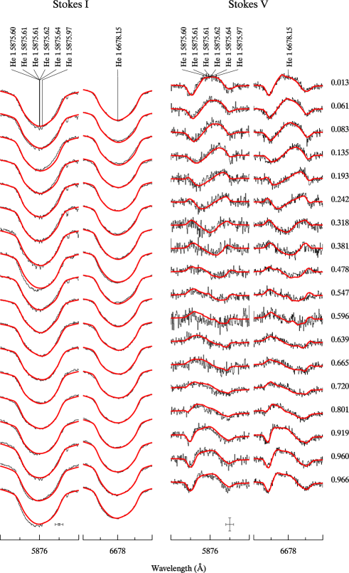
Figure 1: Comparison between observed (black) and computed (red) Stokes $I$ and $V$ profiles of the He i 5876Å and 6678Å lines. Rotational phases are indicated to the right of the Stokes $V$ profiles. Spectra corresponding to consecutive phases are shifted vertically. The bars at the lower left corner of each panel indicate the horizontal (1 Å) and vertical (5 per cent) scales of the profile plots.

A small percentage of main sequence A- and B-type (Ap/Bp) stars are characterized by peculiar surface abundances of chemical elements and strong (0.1-30 kG), large-scale magnetic fields. These magnetic Ap/Bp stars exhibit periodic variability of spectral lines, photometric brightness, and longitudinal magnetic field strength that is explained in the context of the Oblique Rotator Model (ORM) described by Stibbs (1950). The peculiar element abundances present themselves in the form of inhomogeneous, asymmetric “spots” on the surface of the star, causing spectral line shape and strength variability, and in some cases photometric brightness variations, all modulated on the stellar rotation period. These inhomogeneities on the surface of magnetic chemically peculiar stars are thought to be formed by direct or indirect interactions between chemical diffusion and the stabilizing influence of magnetic field lines (see e.g., Michaud, 1970).

The technique of Doppler imaging (DI) was originally used by Goncharskij et al. (1982) to map the abundance of a chemical element on the surface of a star assuming rotational variability of line profiles with time. This simple, yet elegant method of studying stellar spots was eventually extended to simultaneously map both chemical abundances as well as a star’s surface magnetic field. This method, magnetic Doppler imaging (MDI), was previously employed to study Ap/Bp stars, and successfully investigates both the surface inhomogeneities of various elements and the magnetic field topology. The MDI code INVERS10 was developed by Piskunov & Kochukhov (2002) to accurately model stellar magnetic fields and surface abundance features from an inversion of high resolution spectropolarimetry. The code was originally developed to operate with data in all four Stokes parameters. However, it is also able to handle a set of data comprised of only Stokes $I$ and $V$ spectra.

Using abundance maps derived from DI, Krtička et al. (2007) showed that both the photometric and spectroscopic variability of another He-strong star, HD 37776, can be explained by the presence of inhomogeneous abundances across the stellar surface. Similar work corroborates this claim for the case of the rapidly rotating Ap star CU Vir (Krtička et al., 2012). Krtička et al. (2013) determined that the photospheric spots of HD 64740 are not sufficient to cause detectable photometric variability. Further, these authors identified UV line variability due to these spots, without any evidence of circumstellar features.

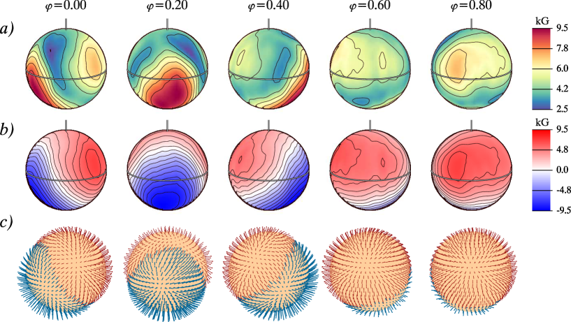
Figure 2: Surface magnetic field distribution derived for $\sigma$ Ori E with magnetic DI. The star is displayed at five equidistant rotational phases as indicated at the top of the figure. The rotational axis is indicated by the short vertical bar, while the thick line shows the stellar rotational equator. The maps correspond to an inclination angle $i=75$°and a $v_{\text{rot}}\sin i=140$ km s^-1. a): Maps of the magnetic field modulus. The contour lines are plotted with a step of 1.0 kG. b): Maps of the radial magnetic field strength. The contour lines are also plotted with a step of 1.0 kG. c): Orientation of magnetic field vectors. In the vector maps, light (red) arrows point outward from the stellar surface. Dark (blue) arrows correspond to vectors pointing inwards. The arrow length is proportional to the field strength.

$\sigma$ Orionis E (HD 37479), the prototypical magnetic He-strong Bp star, has long been known to exhibit variable line profiles, indicating an inhomogeneous surface distribution of various elements. The discovery of its magnetic field by Landstreet & Borra (1978) suggested that this star was a higher mass extension of the Ap/Bp phenomena, and could be physically represented by the ORM. A study by Reiners et al. (2000) modeled historical and new spectra to investigate line profile variations to determine their relationship to local differences of element abundances. The authors found regions of He overabundance and metal (C ii and Si iii) underabundance slightly offset from each other, suggested to be located at the magnetic poles.

Walborn (1974) had discovered broad, variable H$\alpha$ emission features, which, when considered in the context of the ORM, indicated that the emitting material was magnetospheric in nature (Landstreet & Borra, 1978). Various authors worked to develop realistic magnetospheric models for this and other similar stars, with the most recent being the development of the Rigidly Rotating Magnetosphere (RRM) model by Townsend & Owocki (2005). The model analytically describes a rapidly rotating star surrounded by plasma trapped in its magnetosphere. Although the RRM model was relatively successful in reproducing the magnetospheric spectral and photometric variability of $\sigma$ Ori E (Townsend, Owocki & Groote, 2005), major inconsistencies remained.

To begin addressing these issues and the revision of the RRM model, Oksala et al. (2012, hereafter referred to as Paper I) presented and analyzed high resolution intensity and circular polarization spectra $\sigma$ Ori E. These spectra identified various spectral lines that exhibited significant variability and presented an updated magnetic field characterization, suggesting a more complex, higher order field structure. This result was in strong contradiction with the offset dipole configuration adopted for the specific case of $\sigma$ Ori E by Townsend, Owocki & Groote (2005).

A remaining issue with the RRM model, which we aim to address here, are persistent discrepancies between the observed optical photometric light curve and the model light curve (see for example Figure 8, this paper). As noted by Townsend, Owocki & Groote (2005), a significant observed feature of increased brightness is unmatched at rotational phase 0.6 (see their Fig. 1). As these authors invoked the de-centered dipole as a means to mimic the unequal depths of the light minima, a change of the magnetic configuration would cause changes to the synthetic light curve, and further differences will likely arise in the model-observation comparison. The most precise photometric data to date were obtained over a period of three weeks with the MOST micro-satellite, and were presented and analyzed by Townsend et al. (2013). The emission and absorption features previously seen in the light curve of $\sigma$ Ori E are clearly present, and support the notion that these features are real, and also stable. The properties of the two minima strongly differ, with one eclipse deeper than the other, while the more shallow feature is present during a longer portion of the rotation period. The excess brightness at phase 0.6 is quite evident, and the high precision reveals a gradual decline of this excess before returning to the “continuum” level.

This subsequent work continues our re-evaluation of the RRM model, utilizing cutting edge techniques to analyze the magnetic and abundance structure of $\sigma$ Ori E via MDI, revise the RRM model, and, through a thorough light curve analysis, address any remaining discrepancies between model and observation. Section 2 explains the MDI procedure and results. Section 3 presents the revised RRM model. We discuss in Section 4 the light curve analysis of the optical photometry. An analysis of UV variability is explored in Section 5. Section 6 presents a summary of this paper.

2 Magnetic field and elemental abundance mapping

2.1 Magnetic Doppler imaging (MDI)

For input into MDI, we obtained a total of 18 high-resolution (R=65000) broadband (370-1040 nm) Stokes $I$ and $V$ spectra of $\sigma$ Ori E. Sixteen spectra were obtained in November 2007 with the Narval spectropolarimeter on the 2.2m Bernard Lyot telescope (TBL) at the Pic du Midi Observatory in France. The remaining two spectra were obtained in February 2009 with the spectropolarimeter ESPaDOnS on the 3.6-m Canada-France-Hawaii Telescope (CFHT), as part of the Magnetism in Massive Stars (MiMeS) Large Program (Wade et al., 2011). The observations and their reduction are described in more detail in Paper I.

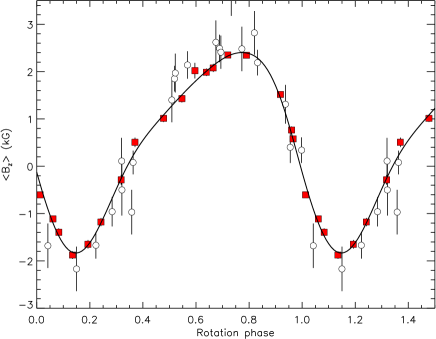
Figure 3: Longitudinal magnetic field measurements (red filled squares) for $\sigma$ Ori E (Paper I), as well as data reported in Landstreet & Borra (1978) and Bohlender et al. (1987) (open circles). Each data point is plotted with corresponding 1$\sigma$ error bars. The solid curve is the longitudinal magnetic field curve computed using the MDI-derived magnetic field structure. The data are phased using the ephemeris of Townsend et al. (2010).

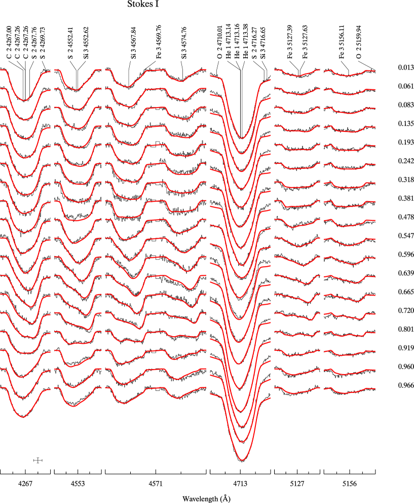
Figure 4: Comparison between observed (black) and computed (red) Stokes $I$ profiles of lines used for chemical abundance mapping.. Rotational phases are indicated to the right of the profiles. Spectra corresponding to consecutive phases are shifted vertically. The bars at the lower left corner of each panel indicate the horizontal (1 Å) and vertical (5 per cent) scales of the profile plots.

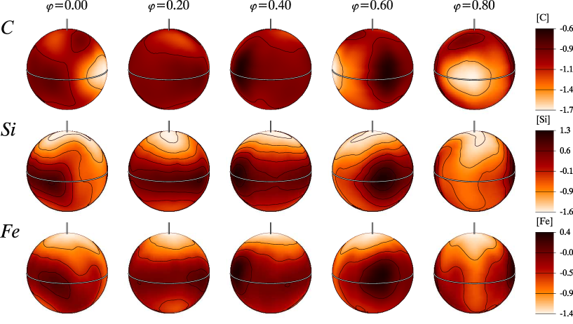
Figure 5: The chemical abundance distributions of C, Fe, and Si derived from Stokes $I$ line profiles. The star is shown at 5 equidistant rotational phases viewed at the inclination angle, $i=75\degr$ and $v\sin i=140$ km s^-1. The scale gives abundance as $\epsilon_{Elem}$ corresponding to $\log(\rm{N}_{Elem}/\rm{N}_{tot})$ relative to solar values. The rotation axis is vertical. The contour step size is 0.5 dex.

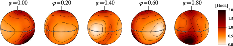
Figure 6: The chemical abundance distribution of He derived from Stokes $I$ line profiles of the 4713 Å He i line. The star is shown at 5 equidistant rotational phases viewed at the inclination angle, $i=75\degr$ and $v\sin i=140$ km s^-1. The scale gives abundance as $\log(\rm{He}/\rm{H})$ relative to solar values. The rotation axis is vertical. The contour step size is 0.5 dex.

In this work, we utilize the INVERS10 MDI code (Piskunov & Kochukhov, 2002) and its recent derivative INVERS13 (Kochukhov, Wade & Shulyak, 2012; Kochukhov et al., 2013) to reconstruct the surface abundance distribution and magnetic field topology of $\sigma$ Ori E using these high-resolution Stokes $I$ and $V$ spectra. Both codes use least-squares minimization together with a regularization procedure to fit synthetic spectra to spectropolarimetric observations. The model spectra are adjusted until the solution converges to the simplest surface distribution that properly describes the observational data.

Because only Stokes $I$ and $V$ spectra were obtained, the final magnetic field solution is not unique, and the choice of regularization becomes important. As described by Piskunov & Kochukhov (2002), without Q and U spectra, we must use an additional a priori constraint, multipolar regularization, which constrains the results according to agreement with a best fit multipolar model magnetic field. Additionally, Stokes $IV$ observations only provide information about the global magnetic field geometry, and is thus unable to reveal small-scale magnetic field structures, such as those seen in some full Stokes $IQUV$ inversions of Ap stars (e.g., Kochukhov et al., 2004; Kochukhov & Wade, 2010; Silvester, Kochukhov & Wade, 2014) We also include the longitudinal field curve as an additional constraint in magnetic inversion following the procedure described by Kochukhov et al. (2002). The resulting field configuration is computed as part of the multipolar regularization procedure. Thus, the multipolar parameters reported here represent an approximation of the 2-D MDI magnetic map, which is derived without using the spherical harmonic parameterization.

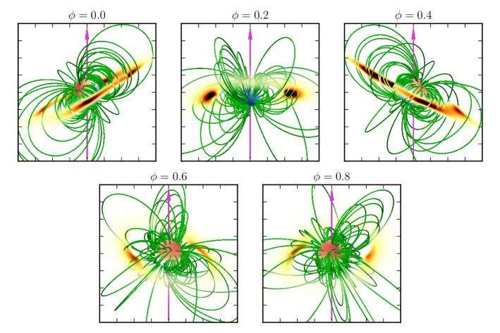
Figure 7: Visualizations of the plasma distribution predicted by the ARRM model, at the same 5 rotational phases adopted in previous figures. The star is colored according to the radial magnetic field strength, as in the middle panels of Fig. 2; selected field lines are plotted in green, and the magenta arrow shows the star’s rotation axis. The surrounding distribution of magnetospheric material is shown via an orange-colored volume rendering, with the more opaque parts corresponding to higher column densities and vice-versa. The tick marks on the surrounding boxes are spaced by $1\,R_{*}$.

2.2 Magnetic field topology

To determine the magnetic field topology of $\sigma$ Ori E, the line profiles of the He i lines at 5876 Å and 6678 Å were chosen for the inversion process. These lines both have strong magnetic signatures in their Stokes $V$ spectrum, while other possible lines exhibit much weaker polarization features, and are therefore less suitable for use in magnetic inversion. We use as input the parameters (${{T}_{\mathrm{eff}}}$, ${\log g}$, and $v_{\text{rot}}\sin i$) determined in Paper I, which are listed in Table 1. The rotational period, $P_{\rm{rot}}$, was derived by Townsend et al. (2010). While these parameters are rather well established for $\sigma$ Ori E, there is a large uncertainty in the determination of the inclination angle, $i$. This is a result of uncertainty in the size and distance of the star, and as such the radius. A range of radius values have been reported via various methods, and so we compute MDI maps at 4 fixed inclination angles to understand the effect of this parameter. Corresponding to a range in radii of 3.3-4.0 R_⋆, models were computed for $i$ = 55, 65, 75, and 85°. This range is adopted based on the discussion of the stellar radius in the Appendix of Townsend et al. (2013), accounting for approximate uncertainties in the angular diameter (Groote & Hunger, 1982) and the cluster distance (Sherry et al., 2008).

While the INVERS10 code relies on LTE model atmospheres, this assumption is not always realistic. For hot stars, the LTE assumption begins to break down starting at T${}_{\rm{eff}}>15000$ K (Mihalas & Athay, 1973), beginning with visibly different line profile strengths and/or shapes. These effects become particularly noticeable above T${}_{\rm{eff}}\sim 22000$ K, resulting in growing discrepancies with LTE model spectra in H i lines and He i lines, particularly those in the red-ward part of the optical spectrum (i.e., 5876 and 6678 Å; Przybilla, Nieva & Butler, 2011). Less obvious effects are seen in metal lines and blue-ward He i lines; the study by Przybilla, Nieva & Butler (2011) finds little difference between LTE and NLTE models for these lines. Thus, to properly model the He i lines we have chosen, these changes need to be incorporated into the synthetic spectrum. The implementation of full NLTE radiative transfer into the INVERS suite of codes is not a trivial task, and we proceed to recover the line profile shapes only for lines to be included in the magnetic field determination. The effect of NLTE departure is more severe for red He i lines, however, the magnetic signature is also stronger in these features, making them useful for determining the magnetic configuration. As a solution, we have used the NLTE model atmosphere code TLUSTY (Lanz & Hubeny, 2007) to determine the departure coefficients for the upper and lower atomic levels of the He transitions in question. The code was set to only consider particle conservation and statistical equilibrium to calculate both the population levels and their associated departure coefficients. Departure coefficients were computed for various values of helium abundance with a LTE ATLAS9 (Castelli & Kurucz, 2006) model atmosphere with T${}_{\rm{eff}}=23000$ K and ${\log g}={4.0}$ as the initial input for the TLUSTY computation. Then, during inversion, INVERS10 interpolated departure coefficients for the local value of He abundance and modified the line absorption coefficient and the source function accordingly.

With the longitudinal magnetic field curve derived in Paper I as an additional constraint in addition to the multipolar regularization (Piskunov & Kochukhov, 2002), we obtained a good fit to both the Stokes $I$ and $V$ line profiles of the two He i lines, shown in Figure 1. These figures correspond to an inclination of $i$ = 75°. The best fit magnetic field configuration over the considered range of inclination angles ($i=55-85$°) suggests a magnetic field that can be approximated as a dipole with polar strength $B_{\rm{d}}=7.3-7.8$ kG, with obliquity $\beta_{\rm{d}}=47-59$°  and phase angle $\gamma_{\rm{d}}=97-98$°, and a smaller non-axisymmetric quadrupole component with strength $B_{\rm{q}}=3-5$ kG. Figure 2 shows the surface magnetic field distribution maps derived for $\sigma$ Ori E corresponding to this topology (again, for $i=75$°). The dipole is centered, but the quadrupole axis is misaligned with the dipolar axis, leading to a geometry where the positive and negative poles are clearly not separated by 180°. The asymmetry is further evident in the longitudinal field curve shown in Figure 3, where the observed longitudinal field measurements from all epochs are plotted along with the synthetic curve computed from the MDI magnetic maps. The data are very well matched, and corroborate the conclusions of Paper I, particularly their Figure 7, which shows a comparatively poor fit to the observed data using the original RRM de-centered dipole field configuration.

2.3 Metal abundance

With a magnetic field topology corresponding to an inclination $i=75$°set as a fixed parameter, INVERS10 was then used to compute the distribution of various chemical elements on the surface of the star. This inclination was chosen as it was used for the original $\sigma$ Ori E RRM analysis by Townsend, Owocki & Groote (2005), and we expect far less uncertainty in the determination of the surface fields with varying inclination angle. The set of high resolution time-series spectra of $\sigma$ Ori E contain lines suitable for modeling the abundances of Fe, Si, C, and He. Other chemical elements are present in the spectrum, but their line strength was too weak for accurate determination of any surface structure. He lines required a slightly more rigorous treatment, and will be discussed in the next section.

The Stokes $I$ spectral lines were fit, with the final results shown in Figure 4. There is good agreement between the observations and the model fits for all of these lines. Figure 5 displays spherical maps of the abundance distributions of Fe, Si, and C. The maps of Si abundance were determined using three closely located Si iii lines at 4552.62 Å, 4567.84 Å, and 4574.76 Å. The surface distribution of C was computed from the C ii 4267 Å triplet. Fe maps were produced using the Fe iii doublet lines at 5127.39 and 5127.63 Å and the Fe iii singlet line at 5156.11 Å. The surface maps shown in Figure 5 indicate that Fe, Si, and C all show a similar pattern over the stellar surface. The minimum abundances are found at rotational phase 0.8, in both a spot at the equator and at the visible pole. An equatorial spot at $\sim$ phase 0.6 has the maximum value on the surface.

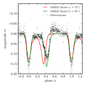
Figure 8: Comparison between the observed (black dots; Hesser et al., 1977) and modeled photometric light curves for $i=75\degr$ (red curve) and $i=85\degr$ (green curve), for the Strömgren $u$-band.

2.4 He abundance

As discussed in Section 2.2, the two helium lines used for magnetic mapping are more sensitive to departure from NLTE. Further, these lines are very strong, and as such they have a weaker ability to diagnose changes in abundance. We find that He i 5876 Å and 6678 Å also contain contamination from the circumstellar material, which was confirmed in Paper I by evaluating the variability of the equivalent widths (EWs) of these lines. We therefore choose to determine the photospheric helium abundance using the weaker He i 4713 Å line, which does not show any distortion due to either NLTE effects or the magnetosphere. Further, instead of using the standard INVERS10 MDI code to compute synthetic He line profiles, we chose to use a different imaging code, INVERS13 (for more details see Kochukhov, Wade & Shulyak, 2012; Kochukhov et al., 2013). This MDI code is capable of computing local Stokes parameter profiles according to local atmospheric conditions, modified by the presence of chemical or temperature spots. In the case of $\sigma$ Ori E, which shows a large He overabundance and a non-uniform surface distribution of this element, we computed a grid of LTE model atmospheres with LLmodels code (Shulyak et al., 2004) for a range of He/H ratios. This grid was then used in modeling of the He i 4713 Å line, allowing us to derive a more accurate He surface map than when using a single mean atmosphere. As with the metals, the He abundance distribution was computed with the fixed magnetic field geometry determined from the red He lines.

Figure 6 shows a He abundance map indicating a large spot of overabundance at phase 0.8, located in the lower hemisphere. This corresponds with the EW variation in the He i 6678 and 5876 Å lines derived in Paper I. The minimum abundance is located at phase 0.6, with a normal, solar level of He. The spot of enhanced He does not appear to be correlated with the location of the magnetic poles. Also of note is the anti-correlation between the strength of metals and He, previously established in Paper I from EW variations.

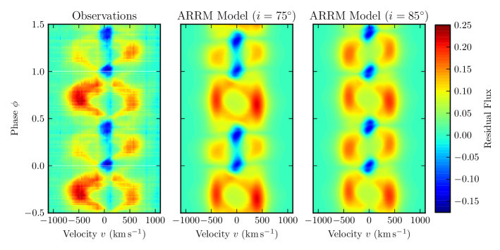
Figure 9: Comparison between observed (left) and modeled (middle and right) H$\alpha$ dynamic spectra of $\sigma$ Ori E, in each case plotting the residual flux as a function of velocity and rotation phase. The middle plot is determined for an inclination angle, $i=75\degr$, while the right plot is the same, but for $i=85\degr$. The observational data and the synthetic reference spectrum used to calculate the residuals are described in Section 4 of paper I.

3 The revised Rigidly Rotating Magnetosphere model for $\sigma$ Ori E

The initial success of applying the Rigidly Rotating Magnetosphere (RRM) model to $\sigma$ Ori E, by Townsend, Owocki & Groote (2005), triggered a renewed era of observational monitoring of this archetypal object, across a range of different wavelengths. In Paper I, we presented the first-ever high-resolution spectropolarimetry of $\sigma$ Ori E, which reveals that the star’s magnetic topology is more complex than assumed in the original RRM analysis. Here, we explore the consequences of this revised topology, considering the analysis of Section 2.2, for the RRM-predicted distribution of circumstellar material.

3.1 The Offset-Dipole RRM Model

The RRM analysis by Townsend, Owocki & Groote (2005) assumed a dipole magnetic topology tilted at an angle $\beta=55^{\circ}$ with respect to the rotation axis and then offset by $0.3\,R_{*}$ in a direction essentially perpendicular to both rotational and magnetic axes. The offset results in an mass/density asymmetry in the predicted magnetospheric mass distribution (with respect to the plane containing both axes), which nicely explains the observed inequalities in the depths of the light-curve minima and the heights of the H$\alpha$ emission peaks.

Townsend, Owocki & Groote (2005) reported that their offset-dipole topology produces a reasonable fit (reduced $\chi^{2}=1.79$) to the longitudinal magnetic field ($B_{\ell}$) measurements available at that time, only marginally worse than a centered dipole. However, a review of the field synthesis code used by these authors has revealed a couple of bugs, which tend to suppress the effects of the offset on the $B_{\ell}$ curve. With these bugs fixed, the predicted $B_{\ell}$ is clearly inconsistent with the observations: the transition from magnetic maximum to minimum is gradual, while the transition from minimum of maximum is quite steep – precisely the opposite of the observed behavior (see Fig. 3).

This mismatch could be partly mitigated by offsetting the dipole in the opposite direction (at the expense of worsening the light curve and H$\alpha$ fits). However, recognizing that an offset dipole is at best a crude approximation to the star’s true magnetic topology, and that we now have access to a more physically realistic topology (Sec.2.2), a better approach is to discard the offset dipole approach and instead extend the RRM model to handle arbitrary non-dipolar fields.

3.2 A New Arbitrary-Field RRM Model

The Arbitrary-Field RRM (ARRM) model is an extension of the original RRM formalism to allow consideration of arbitrary circumstellar field topologies. The theoretical basis remains the same: the distribution of density $\rho$ along a given closed magnetic flux tube is calculated by solving the equation of hydrostatic equilibrium subject to gravitational and centrifugal forces. This yields

$$\rho(s)=\begin{cases}\rho_{0}\exp\left[-\mu\frac{\Phi(s)-\Phi_{0}}{kT}\right]&s_{a}<s<s_{b}\\ 0&\text{otherwise}\end{cases},$$ (1)

where $s$ is the coordinate measuring arc distance along the flux tube; $s_{a}$ and $s_{b}$ are the coordinates of the maxima in the effective potential $\Phi(s)$ that are situated closest to the tube footpoints, and the other symbols have the same meaning as described by Townsend & Owocki (2005). In this expression, which is equivalent to equation (25) of Townsend & Owocki (2005), $\rho_{0}\equiv\rho(s_{0})$ is the density at an arbitrary reference coordinate $s=s_{0}$, and $\Phi_{0}\equiv\Phi(s_{0})$ is the corresponding effective potential.

To determine $\rho_{0}$, we integrate the density distribution (1) along the full length of the flux tube, giving the total mass $m$ in the tube as

$$m=\int_{s_{\rm S}}^{s_{\rm N}}\rho(s)\,{\rm d}A(s)\,{\rm d}s.$$ (2)

Here, ${\rm d}A(s)$ is the nominal cross-sectional area of the tube, and $s_{\rm N}$ and $s_{\rm S}$ are the arc coordinates of the northern ($B_{r}>0$) and southern ($B_{r}<0$) tube footpoints, respectively. Conservation of magnetic flux requires that

$$|\mathbf{B}(s)|\,{\rm d}A(s)=|\mathbf{B}(s_{\rm N})|\,{\rm d}A(s_{\rm N})=|\mathbf{B}(s_{\rm S})|\,{\rm d}A(s_{\rm S}).$$ (3)

Likewise, conservation of mass requires that

$$m=\dot{m}t,$$ (4)

where $\dot{m}$ is the rate at which mass is being added to the tube, and $t$ is the time elapsed since the magnetosphere last began to refill. Generalizing equation (31) of Townsend & Owocki (2005), the filling rate $\dot{m}$ can be related to the global CAK mass-loss rate $\dot{M}$ via

$$\dot{m}=\frac{\dot{M}}{4\pi R_{*}}\left(\frac{B_{r}(s_{\rm N})}{|\mathbf{B}(s_{\rm N})|}\,{\rm d}A(s_{\rm N})+\frac{B_{r}(s_{\rm S})}{|\mathbf{B}(s_{\rm S})|}\,{\rm d}A(s_{\rm S})\right)$$ (5)

With the arbitrarily chosen timescale $t$ setting the overall mass contained in the magnetosphere, and for given stellar parameters and magnetic topology, these equations suffice to calculate the density everywhere in the magnetosphere.

Figure 10: Upper plot: The dependence of temperature on the Rosseland optical depth $\tau_{\text{ross}}$ in a reference model atmosphere with a slightly overabundant chemical composition ($\varepsilon_{\text{He}}=-1.0$, $\varepsilon_{\text{C}}=-4.1$, $\varepsilon_{\text{Si}}=-4.1$, and $\varepsilon_{\text{Fe}}=-4.7$). Lower plot: The relative change of the temperature in the model atmospheres with modified abundance.

3.3 Applying the ARRM Model to $\sigma$ Ori E

Figure 11: Upper plot: The emergent flux from a reference model atmosphere with slightly overabundant chemical composition ($\varepsilon_{\text{He}}=-1.0$, $\varepsilon_{\text{C}}=-4.1$, $\varepsilon_{\text{Si}}=-4.1$, and $\varepsilon_{\text{Fe}}=-4.7$). Lower plot: The emergent flux from the model atmospheres with modified abundance of individual elements minus the flux from the reference model. A magnified section of the lower plot showing the redistribution of flux to longer wavelengths is over-plotted in the small upper panel. All fluxes were smoothed by a Gaussian filter with a dispersion of $10\,$Å to show the changes in continuum, a major contribution to SED variability.

Applying the ARRM model to $\sigma$ Ori E requires a prescription for the magnetic field vector $\mathbf{B}$ throughout the magnetosphere. To this end, we extrapolate from the surface radial field distribution using the potential-based approach described by Jardine et al. (2002). This method is employed with the assumption that the field remains strongly dominant over the wind to a distance within which the majority of the material is located. As can be seen directly in Fig. 9, the material responsible for the H$\alpha$ emission is located in a radius range of $\sim$2-4 R_∗. Since the density is a strong function of radius, we expect the amount of material in the magnetosphere to greatly decrease with distance from the star. This agrees with the bulk of the material being located close to the Keplerian co-rotation radius, which is consistent with the results of MHD simulations by ud-Doula et al. (2008). Moreover, at this distance, the magnetic tension dominates the centrifugal force by a factor of $\sim 10^{3}$, assuring minimal distortion from a pure dipole form. The determination of where the balance between these forces becomes more equal, and how it determines the size and shape of the disc are issues that, along with further details about the implementation of this extrapolation, will be given in a forthcoming paper (Townsend et al., in prep.).

Figure 7 presents visualizations of the magnetic topology and the associated density distribution predicted by the ARRM model for $\sigma$ Ori E, at the same five rotation phases illustrated in Figs. 2 and 4, for an inclination angle $i=75\degr$. The material in the magnetosphere is distributed in an oblique, warped disk-like structure, qualitatively the same as shown Fig. 4 of Townsend, Owocki & Groote (2005) for a simple oblique dipole. This is not unexpected — the rapid falloff of higher-order components means that the field in the ARRM model, at the distances $r\gtrsim 2\,R_{*}$ where the material is situated, is close to dipolar. The model simulations keep free the parameter which designates the total amount of material in the magnetosphere, so that the observations can be best matched. The model used here indicates a mass density within the magnetosphere of $5\times 10^{-12}$ g cm^-3, or a number density of $5\times 10^{12}$ cm^-3.

The light curve and H$\alpha$ dynamic spectrum predicted by the ARRM model are compared against the corresponding observational data in Figs. 8 and 9. The photometric data are Strömgren $u$ band taken by Hesser et al. (1977). The observed H$\alpha$ spectra are part of the data presented here and in Paper I. The approach used to calculate these observables is similar to that described by Townsend, Owocki & Groote (2005), except that we now include an NLTE photospheric line profile (as described in Sec. 4.1 of Paper I) in the spectral synthesis rather than a flat continuum. The comparison has been shown for both $i=75$ and $85\degr$; we do not show similar plots for $i=55$ or $65\degr$, as they make the comparison much worse, and as such can be ruled out as possible inclination angles. Clearly, the model predictions computed with $i=85\degr$ more closely match the timing of the observed variability, however, a clear difference between observations and model can be seen in Fig. 8: the secondary minimum at $\phi\sim 0.4$ is deeper than the primary minimum at $\phi\sim 0.0$, the opposite of what is seen in the observations. This reversal is also apparent in the strength of the H$\alpha$ emission peaks, with the blue peak being stronger than the red one at $\phi\sim 0.75$ in the observations, but vice-versa for the model. We also note that the models do not extend the H$\alpha$ emission out far enough in velocity, particularly on the blue side, something that will be explored in the next iteration of this model. Furthermore, the improvements added to develop the ARRM model are not sufficient to explain the enhanced emission at phase 0.6.

4 Photospheric contribution to the optical brightness variation

The previous section (Sec.3.3) demonstrates that the current version of the RRM model, the ARRM model, is not effective at explaining the totality of the features seen in the optical variability of $\sigma$ Ori E. However, the model is strictly accounting for the circumstellar contribution to these observables, without consideration of any other possible contribution to the variability. In the following sections, we explore the contribution from the stellar photosphere, accounting for the effects of an inhomogeneous abundance distributions of several elements.

4.1 Simulation of the SED variability

Table 1: Adopted physical parameters of $\sigma$ Ori E. Table references: ¹Oksala et al. (2012), ²Townsend et al. (2010).

Effective temperature ${{T}_{\mathrm{eff}}}$1	${23\,000}\pm 3\,000$ K
Surface gravity ${\log g}$ (cgs)1	${4.0}\pm 0.5$
Projected rotational velocity $v_{\text{rot}}\sin i$1	$140\pm 10\,\text{km}\,\text{s}^{-1}$
Rotational period Prot2	$1\aas@@fstack{d}1908229+1\aas@@fstack{d}44\times 10^{-9}E$
Helium abundance	$-1.1<\varepsilon_{\text{He}}<0.6$
Carbon abundance	$-5.0<\varepsilon_{\text{C}}<-4.0$
Silicon abundance	$-5.9<\varepsilon_{\text{Si}}<-3.2$
Iron abundance	$-5.7<\varepsilon_{\text{Fe}}<-4.0$

4.1.1 Model atmospheres and synthetic spectra

The simulation of the ultraviolet and visual SED variability primarily utilizes the NLTE model atmosphere code TLUSTY (Hubeny, 1988; Hubeny & Lanz, 1992, 1995; Lanz & Hubeny, 2003). The atomic data (adopted from Lanz & Hubeny, 2007) are appropriate for B-type stars. These data were originally calculated within the Opacity and Iron Projects (Seaton et al., 1992; Hummer et al., 1993). The calculations assume fixed values of the effective temperature and surface gravity for $\sigma$ Ori E (according to Table 1), and adopt a generic value of the microturbulent velocity $v_{\text{turb}}=2\,\text{km}\,\text{s}^{-1}$. The abundances of helium, carbon, silicon, and iron were taken from the four-parameter abundance grid given in Table 2 covering the range of abundances found on the $\sigma$ Ori E surface as inferred from the MDI mapping discussed in Sections 2.3 and 2.4. Abundances relative to hydrogen were used, i.e., $\varepsilon_{\text{el}}=\log\left(N_{\text{el}}/N_{\text{H}}\right)$. All other elements were set to their solar (Asplund et al., 2005) values.

Synthetic spectra were calculated using the SYNSPEC code for the same parameters (effective temperature, surface gravity, and abundances) and transitions as the model atmosphere calculations. Additionally, we included lines of all elements with atomic number $Z\leq 30$ not included in the model atmosphere calculation. Angle-dependent intensities, $I(\lambda,\theta,\varepsilon_{\text{He}},\varepsilon_{\text{C}},\varepsilon_{\text{Si}},\varepsilon_{\text{Fe}})$, were computed for $20$ equidistantly spaced values of $\cos\theta$, where $\theta$ is the angle between the normal to the surface and the line of sight.

The generation of the complete grid of the model atmospheres and angle-dependent intensities (Table 2) would require calculation of 700 model atmospheres and synthetic spectra. Because not all abundance combinations correspond to physical conditions determined by the abundance maps, we calculated only those models that were realistic. This helped us to reduce the number of calculated models by about two thirds.

Table 2: Individual abundances $\varepsilon_{\text{He}}$, $\varepsilon_{\text{C}}$, $\varepsilon_{\text{Si}}$, and $\varepsilon_{\text{Fe}}$ of the model grid

He	$-1.0$	$-0.5$	$0.0$	$0.5$	$1.0$
C	$-5.1$	$-4.6$	$-4.1$	$-3.6$
Si	$-6.1$	$-5.6$	$-5.1$	$-4.6$	$-4.1$	$-3.6$	$-3.1$
Fe	$-5.7$	$-5.2$	$-4.7$	$-4.2$	$-3.7$

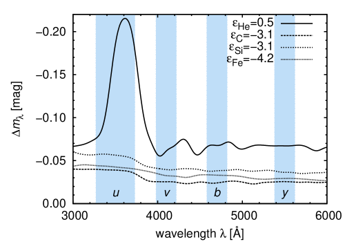
Figure 12: The magnitude difference $\Delta m_{\lambda}$ between the emergent fluxes calculated with enhanced abundance of individual elements and the reference flux $H_{\lambda}^{\text{ref}}$ (see Eq. 9). The fluxes were smoothed by a Gaussian filter with a dispersion of $100\,$Å.

4.1.2 Calculation of phase dependent SED

The radiative flux transmitted through a photometric band $c$ at a distance $D$ from a star with radius $R_{*}$ is (Mihalas, 1978)

$$f_{c}=\left(\frac{R_{*}}{D}\right)^{2}\!\!\int\limits_{\begin{array}[]{c}\text{\scriptsize visible}\\[-5.69054pt] \text{\scriptsize surface}\end{array}}\!\!I_{c}(\theta,\Omega)\cos\theta\,\text{d}\Omega.$$ (6)

The specific band intensity $I_{c}(\theta,\Omega)$ is obtained by interpolating between intensities $I_{c}(\theta,\varepsilon_{\text{He}},\varepsilon_{\text{C}},\varepsilon_{\text{Si}},\varepsilon_{\text{Fe}})$ for abundances found at the surface point with spherical coordinates $\Omega$. These intensities are calculated from the grid of synthetic spectra (see Table 2) according to

$$I_{c}(\theta,\varepsilon_{\text{He}},\varepsilon_{\text{C}},\varepsilon_{\text{Si}},\varepsilon_{\text{Fe}})=\int_{0}^{\infty}\Phi_{c}(\lambda)\,I(\lambda,\theta,\varepsilon_{\text{He}},\varepsilon_{\text{C}},\varepsilon_{\text{Si}},\varepsilon_{\text{Fe}})\,\text{d}\lambda.$$ (7)

The response function $\Phi_{c}(\lambda)$ for individual bands is derived by either fitting the tabulated response functions or simply assuming a Gaussian function.

The magnitude difference in a given band is defined as

$$\Delta m_{c}=-2.5\,\log\,\left(\frac{{f_{c}}}{f_{c}^{\mathrm{ref}}}\right),$$ (8)

where $f_{c}$ is calculated from Eq. 6 and ${f_{c}^{\mathrm{ref}}}$ is the reference flux obtained under the condition that the mean magnitude difference over the rotational period is zero.

4.2 Influence of abundance on emergent flux

Figure 13: Predicted light variations of $\sigma$ Ori E in the Strömgren photometric system calculated considering only the variations of individual elements. The abundance of other elements was fixed. Light curves in individual filters were vertically shifted to better demonstrate the light variability.

The bound-free and bound-bound transitions of individual elements can modify the temperature of model atmospheres. This can be seen in Fig. 10, where we compare the temperature distribution of model atmospheres for typical overabundances of $\sigma$ Ori E to the distribution for abundances slightly higher than solar. The bound-free (due to ionization of helium, carbon, and silicon) and bound-bound (line transition of iron) transitions absorb the stellar radiation, consequently the temperature in the continuum forming region ($\tau_{\text{ross}}\approx 0.1-1$) increases with increasing abundance of these elements. In the uppermost layers $\tau_{\text{Ross}}\lesssim 10^{-3}$, the stronger line cooling in the models with enhanced abundance leads to the decrease of the atmosphere temperature.

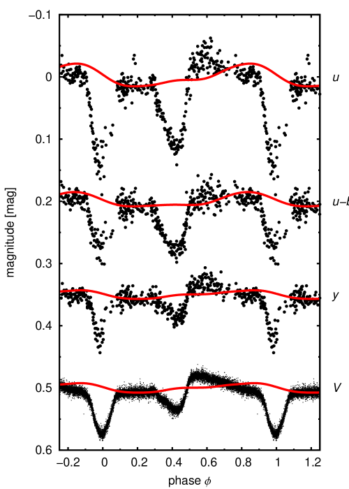
Figure 14: Predicted light variations of $\sigma$ Ori E (solid lines) computed taking into account helium, silicon, carbon, and iron surface abundance distributions. Light curves in individual filters were vertically shifted to better demonstrate the light variability. The top three light curves are from the Strömgren photometric system, with the data again that of Hesser et al. (1977). The bottom light curve is calculated for the wide-band visual filter corresponding to the MOST data (Townsend et al., 2013).

In atmospheres with overabundant helium, carbon, silicon or iron, enhanced opacity leads to the redistribution of the flux from the short-wavelength part of the UV spectrum to longer wavelengths, and also to the visible spectral regions (see Figure 11 and Krtička et al., 2007). Consequently, overabundant spots are typically bright in the visual and near UV bands, and are dark in the far UV bands.

These flux changes can be detected in the variability of the SED and particularly in the variability of visible light. To demonstrate the optical variations, we plot (Fig. 12) the relative magnitude difference

$$\Delta m_{\lambda}=-2.5\log\left(\frac{H_{\lambda}(\varepsilon_{\text{He}},\varepsilon_{\text{C}},\varepsilon_{\text{Si}},\varepsilon_{\text{Fe}})}{H_{\lambda}^{\text{ref}}}\right),$$ (9)

against wavelength. Here $H_{\lambda}^{\text{ref}}$ is the reference flux calculated for slightly overabundant chemical composition (with $\varepsilon_{\text{He}}=-1.0$, $\varepsilon_{\text{C}}=-4.1$, $\varepsilon_{\text{Si}}=-4.1$, and $\varepsilon_{\text{Fe}}=-4.7$). As can be seen in Figure 12, the absolute value of the relative magnitude difference is the largest in the $u$-band of the Strömgren photometric system, while it is nearly the same in the visual bands, $v$, $b$, and $y$-band. The strong maximum in the $u$-band model with enhanced helium is caused by the filling of the Balmer jump. In the helium rich models, the jumps due to hydrogen diminish, while the jumps due to helium become visible.

4.3 Predicted visual light variations

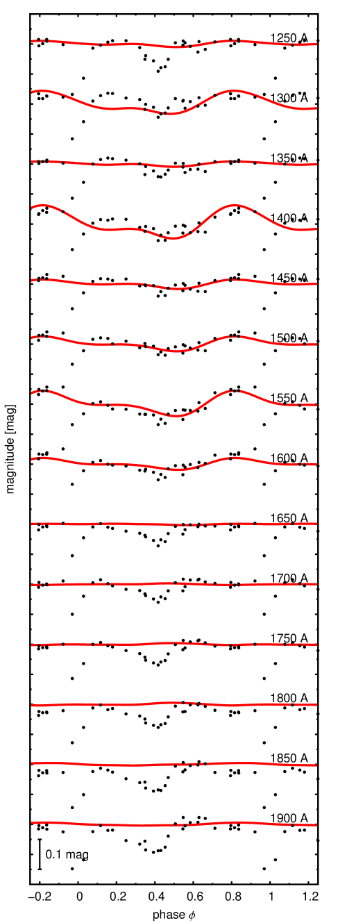
Figure 15: Comparison of the predicted (solid line) and observed (dots) UV light variations for different wavelengths. Curves for individual wavelengths were vertically shifted to better demonstrate the variability.

Predicted light curves are calculated from the surface abundance maps derived using MDI in Section 2 and from the emergent fluxes computed with the SYNSPEC code, applying Eq. 8 for individual rotational phases.

To study the influence of individual elements separately, we first calculated the light variations with the abundance map of a single element (Fig. 13), assuming a fixed abundance of other elements ($\varepsilon_{\text{He}}=-1.0$, $\varepsilon_{\text{C}}=-4.1$, $\varepsilon_{\text{Si}}=-4.1$, $\varepsilon_{\text{Fe}}=-4.7$). Fig. 13 shows that helium, iron, and silicon contribute predominantly to the light variations, while the contribution of carbon is only marginal. This is due to the large overabundance of these elements within the spots and their large abundance variations on the stellar surface. The amplitude of the light variations is the largest in the Strömgren $u$-band, as expected from Fig. 12. Because the overabundant regions are brighter in the $uvby$ colors, the predicted light variations reflect the equivalent width variations. The light maximum occurs at the same phase at which the equivalent width of a given element is the greatest. Helium lines are strongest for phase 0.8, consequently the light curve due to helium shows its maximum at phase 0.8. Iron and silicon lines are strongest for phase 0.6, consequently the light curve due to both iron and silicon shows its maximum at phase 0.6.

Incorporating the surface distributions of helium, carbon, silicon, and iron in the calculation of light curves (Fig. 13), we obtain the results given in Figure 14. Helium, due to its large overabundance, dominantly influences the light curve of $\sigma$ Ori E. This is the opposite behavior seen for HD 37776, where silicon was the main cause of the light variability (Krtička et al., 2007). This is due to the higher silicon abundance in HD 37776 by about 0.8 dex.

The observed visual light curve of $\sigma$ Ori E has a maximum at phase $\sim$0.6, when the iron lines are the strongest (Fig.14), however, the model indicates the light curve has a maximum for the phase of about 0.8 when the helium lines are the strongest. Consequently, the observations strongly disagree with theory in the optical region, and the excess brightness at phase 0.6 cannot be explained as an effect of inhomogeneous surface abundance of considered elements.

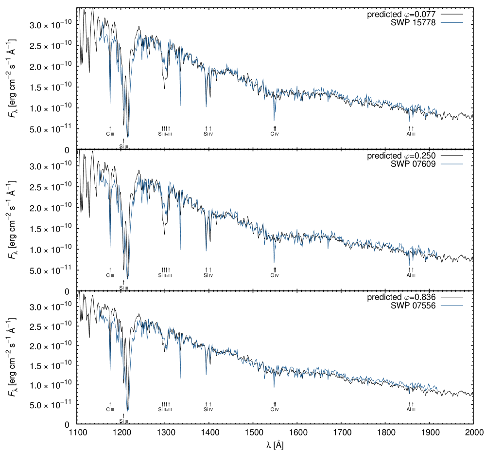
Figure 16: Comparison of observed (IUE) and predicted fluxes in the UV region for selected phases. The predicted flux was smoothed by a Gaussian filter with dispersion 1.3 Å, which roughly corresponds the the IUE data.

5 Extended analysis of the UV variability

The light variability caused by the uneven distribution of elements on the surface of $\sigma$ Ori E is connected with the flux redistribution from the far UV to the near UV and visible regions (see e.g., Figure 11). Consequently, the light variability in the far UV region provides an important test of the light variability mechanism. To test these predictions quantitatively, we extracted IUE observations of $\sigma$ Ori E from the INES database (Wamsteker et al., 2000) using the SPLAT package (Draper, 2004, see also Škoda 2008). Here we use low-dispersion large aperture spectra in the domain 1250–1900 Å (SWP camera).

5.1 Narrow band UV variations

As a first comparison of the UV fluxes, we focused on narrow band variations. The observed and predicted fluxes were both smoothed with a Gaussian filter with a dispersion of $25\,$Å. The resulting predicted and observed UV variations are given in Fig. 15. Unlike the visible region, light curves calculated from the MDI-derived abundance maps are able to explain at least the main trends of UV light variability of $\sigma$ Ori E. At 1250 Å and 1900 Å  light variability is dominated by light absorption in the circumstellar environment. The observed light curve is nearly constant in the periods between the occultations, with the calculated light curve also producing little variability. Conversely, there are significant variations of the observed flux at 1400 Å and 1550 Å. These variations can be relatively nicely reproduced by our models. The light variability in these regions is mainly due to silicon and iron, while helium does not significantly influence the light variability in the UV region.

5.2 UV flux variations

The variability of the UV spectral energy distribution in Figure 16 is only marginal. The predicted and observed emergent flux distribution agree relatively well during ($\varphi=0.077$) and outside ($\varphi=0.250$, $\varphi=0.836$) eclipses. The flux is greatly influenced by numerous iron lines, whose accumulation around $1550\,$Å causes flux depression in this region. A detailed inspection reveals that the predicted flux is somewhat higher than observed in the region $1150-1250\,$Å for all phases. Moreover, the predicted flux is slightly lower than observed in the region $1650-1900\,$Å  during the maximum of the UV flux variability ($\varphi=0.836$). This may possibly be the source of disagreement between the light curves in the optical region.

5.3 UV line variations

The shapes of many weak lines and the resonance lines of Si iv at $\sim 1400\,$Å seem to be well reproduced by the models in Figure 16. On the other hand, the strengths of strong lines of Si ii and Si iii at 1270 Å and $1300\,$Å and the C iv resonance lines are not reproduced by the models. We use the following indices to study line variability:

$$a(\text{C\,{\sc ii} }1336\,\text{\AA}) =m_{1335.2}-\frac{1}{2}\left(m_{1332.0}+m_{1338.75}\right),$$ (10a)

$$a(\text{C\,{\sc iii} }1175\,\text{\AA}) =m_{1175.7}-\frac{1}{2}\left(m_{1169.0}+m_{1181.25}\right),$$ (10b)

$$a(\text{C\,{\sc iii} }1247\,\text{\AA}) =m_{1247.5}-\frac{1}{2}\left(m_{1244.45}+m_{1249.15}\right),$$ (10c)

$$a(\text{C\,{\sc iv} }1548\,\text{\AA}) =m_{1547.9}-\frac{1}{2}\left(m_{1529.45}+m_{1557.95}\right),$$ (10d)

$$a(\text{Si\,{\sc iv}}) =m_{1393.65}-\frac{1}{2}\left(m_{1388.65}+m_{1398.7}\right).$$ (10e)

These indices were used in the analysis of Krtička et al. (2013) for HD 64740, who modified a similar set of indices developed by Shore, Brown & Sonneborn (1987). Figure 17 compares the observed and predicted variations of the line indices with respect to their mean values. We are able to explain the variations of many individual carbon and silicon lines. The disagreement between predicted and observed line profiles of Si ii and Si iii could be caused by an inhomogeneous vertical distribution of silicon in the atmosphere. The observed line strengths of C iv at $1548\,$Å and $1551\,$Å are significantly larger than predicted. The observed asymmetry of these lines with extended blue wings at each phase indicates formation in the wind. The line strength variations result from the variations of wind mass-flux on the stellar surface. Enhanced absorption in the C ii line at 1336 Å, C iv lines, and Si iv lines observed around the phase $\varphi\approx 0$ possibly originates in the corotating magnetospheric clouds.

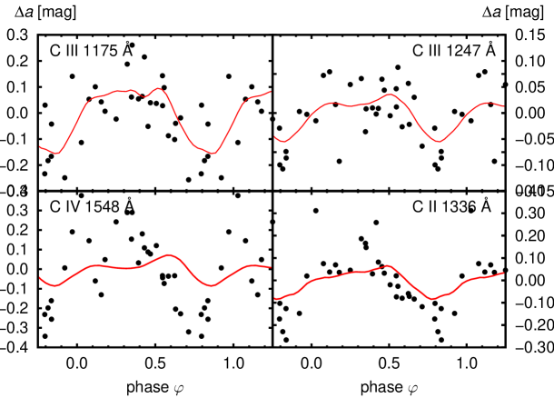
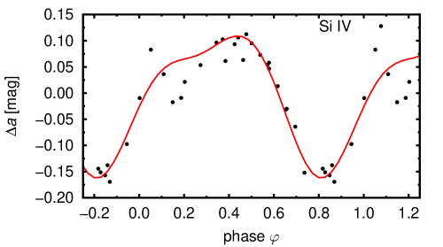
Figure 17: Observed variability of the line indices (dots) in comparison with the predicted indices (lines). Upper panel: Carbon line indices. Lower plot: Silicon line index. The line indices were calculated according to Eq. (10).

6 Confrontation: Round 2

In paper I, we first confronted the RRM model with new high-resolution spectropolarimetry of $\sigma$ Ori E to demonstrate that the field configuration assumed by Townsend, Owocki & Groote (2005) was incompatible with current observations. This first step revealed that more comprehensive modeling was required to explain the intricate physical phenomena of this star. While the initial success of that model is now attributed to a bug in the code, its inspiration has driven studies to better understand the intimate details of the interaction of rotation, magnetic field, and mass-loss, propelling the new wave of high quality data acquisition presented in this and other papers. The current version of the RRM model now does a marginally good job of replicating the qualitative variations of the system, but several discrepancies appear to test the accuracy of the model, and the excess brightness in the optical photometry at phase 0.6 persists.

The magnetic field topology in this application of the ARRM model is taken from the MDI analysis in Section 2.2, and is therefore consistent with the observations of longitudinal magnetic field. Several checks were performed to to ensure that the model adopted the same phasing and rotation as the derived maps, particularly after the discovery of the bug in the initial model. The H$\alpha$ emission comparison is shown in Figure  9, and while the model reproduces much of the variability, there is one glaring inconsistency in the strength of the red-shifted cloud at phase $\sim$0.75. If we carefully inspect the other features throughout the rotation, it seems this one aspect is the only serious problem, indicating the model is predicting too much emitting material in that “cloud” at that particular phase. Likewise, Figure  8 shows a similar reversal in strength of the the model photometric minima with the deeper minimum occurring at the opposite phase as compared to the observed light curve.

Section 4.3 demonstrates clearly there is no photometric resolution to the issue of the excess brightening in the second half of the rotation phase, or the irregular shape of the minimum at phase 0.4, both clearly seen in the MOST photometric light curve. As modeling the photometric contribution to the brightness variability does not resolve the discrepancies, we must at this point consider that the ARRM model is not currently capable of explaining all of the observed variabilities of $\sigma$ Ori E and similar stars in detail, and that additional physics is necessary.

6.1 Where is the missing physics?

Where does this “extra” brightness come from? If we look at Figure 7, geometry could be a possible explanation. Near phase 0.6-0.8, where we see brightening, the magnetosphere is seen more or less pole-on, at which we are able to view all of the emitting surface of the magnetospheric material. At the phase 0.2, we see that the material is viewed more edge-on, with a much less direct view of most of the emitting surface. It is possible (and likely) that the star’s radiation may be reflecting off of the inner edge of the magnetosphere, thus creating a brightening effect. At this iteration, this and other types of scattering are not considered in the RRM model, but likely contribute to the observed brightness. This is extra physics that would need to be implemented into the next version of the code to diagnose the importance and type of scattering that could be responsible, i.e., Rayleigh scattering vs. electron scattering.

Another consideration is the shape of the “clouds”. The ARRM model predicts, for $\sigma$ Ori E, two higher density concentrations within a larger disk-like structure. However, the broadband polarization study of Carciofi et al. (2013) suggests that the material is configured in a much more concentrated structure, much more similar to dumbbells that a disk. A more physically realistic density distribution may present different model predictions. Another effect of the interaction of the star and the magnetic field is the way in which material leaves the surface of the star. In a “normal” OB star, the mass-loss is purely dependent on the strength of the wind, and is proportional to the luminosity. Although the ARRM model considers effects from the magnetic field, the model still assumes standard CAK relations. The influence of strong field lines may modify the mass-loss process, changing the rate at which the material leaves the star resulting in higher or lower mass-loss. The complexity of the field structure may further constrict movement of mass from the surface. An effect like this could be responsible for the discrepancies between the observed H${\alpha}$ emission and the model prediction. Similarly, the influence of the surface abundance inhomogeneities may play an additional role in altering the mass-loss rate.

7 Summary and future work

In the first paper of this series, we evaluated the appropriateness of the magnetic field assumed by Townsend, Owocki & Groote (2005) in which they applied the RRM model to the physical case of $\sigma$ Ori E. The conclusion of that work, that a more complex field was required, served as the motivation for the analyses contained in this subsequent paper. We have used the same high-resolution spectra from Paper I to produce MDI maps of both the magnetic topology and the surface abundance distributions of He, C, Si, and Fe. The derived magnetic topology, which can be represented by a superposition of a dipole plus quadrupole, is consistent with our previous assertion that the field contains higher-order components. This magnetic configuration was then fed into the newly developed arbitrary magnetic field version of the RRM model to re-evaluate the consistency between the model predictions and the observed variations. The resultant predictions qualitatively resemble the observed spectral and photometric variations, but fail to reproduce still several details. While the magnetic field is fixed, the model now predicts a larger density in one of the clouds, which is observed, but located on the wrong side of the star. The new model also does not resolve the previously-identified issues, specifically the excess brightness observed at phase $\sim$0.6.

While clearly some of these issues are related to failings of the model, we proceeded to use the second result of the MDI modeling, the abundance maps, to determine the effect of the surface inhomogeneities on the photometric light curve. With these maps as input, a synthetic light curve was computed with the aid of a grid of stellar atmosphere models. The total resultant light curve, a product of the contributions from He, C, Si, and Fe, provides no solution for the discrepancies between the model and the observations. The light curve is dominated by the He contribution, as this element exhibits the largest variation of abundance across the surface, however, its maximum abundance is viewed at phase 0.8, too late to be helpful in accounting for the feature at phase 0.6. An analysis of the UV light variability shows good agreement between observed variability and computed light curves, however, some narrow wavelength bands are affected by the eclipsing of the magnetospheric material, causing enhanced absorption at similar phases as in the optical.

We thus conclude that the discrepancy between the models and the observations lies in the treatment of the stellar magnetosphere, and that the RRM model must undergo further revision. Adding the ability to accommodate an arbitrary magnetic field topology is just the first step towards our greater understanding of this system, but there are multiple issues to be addressed in future iterations. The inclination angle first and foremost should be determined using all the available information. The model will need to incorporate and test the effects of scattering processes so as to determine their ability to alter the synthetic observations. Tests should be run to understand how the field interacting with the wind could change the stellar mass-loss. When the RRM model was developed, massive star magnetism was just beginning to progress, and at the time, $\sigma$ Ori E was a unique object, the only known member of its class. However, in the past decade, research has grown rapidly, and there are a growing number of stars discovered to have similar properties, and exhibit similar variabilities. By optimizing the RRM model for $\sigma$ Ori E, we can create a blueprint to fully comprehend the physical properties, the interactions within and outside of the star, and the evolutionary implications for this fascinating group of stars.

References

- Asplund et al. (2005) Asplund, M., Grevesse, N., Sauval, A. J., 2005, Cosmic Abundances as Records of Stellar Evolution and Nucleosynthesis, ASP Conf. Ser. 336, eds. T. G. Barnes III, F. N. Bash (San Francisco: ASP), 25
- Bohlender et al. (1987) Bohlender, D. A., Landstreet, J. D., Brown, D. N., & Thompson, I. B., 1987, ApJ, 323, 325
- Carciofi et al. (2013) Carciofi, A. C., Faes, D. M., Townsend, R. H. D. and Bjorkman, J. E., 2013, ApJL, 766, 9
- Castelli & Kurucz (2006) Castelli, F., Kurucz, R. L., 2006, A&A, 454, 333
- Draper (2004) Draper, P. W., 2004, SPLAT: A Spectral Analysis Tool, Starlink User Note 243 (University of Durham)
- Groote & Hunger (1982) Groote, D., Hunger, K., 1982, A&A, 116, 64
- Hesser et al. (1977) Hesser, J. E., Moreno, H., Ugarte, P. P., 1977, ApJL, 216, 31
- Hubeny (1988) Hubeny, I., 1988, Comput. Phys. Commun., 52, 103
- Hubeny & Lanz (1992) Hubeny, I., Lanz, T., 1992, A&A, 262, 501
- Hubeny & Lanz (1995) Hubeny, I., Lanz, T., 1995, ApJ, 439, 875
- Hummer et al. (1993) Hummer D. G., Berrington K. A., Eissner W., Pradhan A. K., Saraph H. E., Tully J. A., 1993, A&A, 279, 298
- Goncharskij et al. (1982) Goncharskij, A. V., Stepanov, V. V., Khokhlova, V. L., Yagola, A. G., 1982, SvA, 26, 690
- Jardine et al. (2002) Jardine, M., Collier Cameron, A., & Donati, J.-F., 2002, MNRAS, 333, 339
- Kochukhov & Piskunov (2002) Kochukhov, O., Piskunov, N., 2002, A&A, 338, 868
- Kochukhov et al. (2002) Kochukhov, O., Piskunov, N., Ilyin, I., Ilyina, S., Tuominen, I., 2002, A&A, 389, 420
- Kochukhov et al. (2004) Kochukhov, O., Drake, N. A., Piskunov, N., de la Reza, R., 2004, A&A, 424, 935
- Kochukhov & Wade (2010) Kochukhov, O., Wade, G. A., 2010, A&A, 513, A13
- Kochukhov, Wade & Shulyak (2012) Kochukhov, O., Wade, G. A., Shulyak, D., 2012, MNRAS, 421, 3004
- Kochukhov et al. (2013) Kochukhov, O., Mantere, M. J., Hackman, T., Ilyin, I., 2013, A&A, 550, A84
- Krtička et al. (2007) Krtička, J., Mikulášek, Z., Zverko, J., Žižňovský, J., 2007, A&A, 470, 1089
- Krtička et al. (2012) Krtička, J., Mikulášek, Z., Lüftinger, T., Shulyak, D., Zverko, J., Žižňovský, J., Sokolov, N. A., 2012, A&A, 537, A14
- Krtička et al. (2013) Krtička, J., Janík, J., Marková, H., Mikulášek, Z., Zverko, J., Prvák, M., Skarka, M., 2013, A&A, 556, A18
- Lanz & Hubeny (2003) Lanz, T., Hubeny, I., 2003, ApJS, 146, 417
- Lanz & Hubeny (2007) Lanz, T., Hubeny, I., 2007, ApJS, 169, 83
- Landstreet & Borra (1978) Landstreet, J. D., Borra, E. F., 1978, ApJL, 224, 5
- Michaud (1970) Michaud, G., 1970, ApJ, 160, 641
- Mihalas (1978) Mihalas D., 1978, Stellar Atmospheres (San Francisco: Freeman & Co., 1978)
- Mihalas & Athay (1973) Mihalas D., Athay, R.G., 1973, ARA&A, 11, 187
- Oksala et al. (2012) Oksala, M. E., Wade, G. A., Townsend, R. H. D., Owocki, S. P., Kochukhov, O., Neiner, C., Alecian, E., Grunhut, J., 2012, MNRAS, 419, 959
- Piskunov & Kochukhov (2002) Piskunov, N., Kochukhov, O., 2002, A&A, 381, 736
- Przybilla, Nieva & Butler (2011) Przybilla, N., Nieva, M.-F., Butler, K., 2011, J. Phys.: Conf. Ser., 328, 012015
- Reiners et al. (2000) Reiners, A., Stahl, O., Wolf, B., Kaufer, A., & Rivinius, T., 2000, A&A, 363, 585
- Seaton et al. (1992) Seaton, M. J., Zeippen, C. J., Tully, J. A., et al. 1992, Rev. Mexicana Astron. Astrofis., 23, 19
- Sherry et al. (2008) Sherry, W. H., Walter, F. M., Wolk, S. J., Adams, N. R., 2008, AJ, 135, 1616
- Shore, Brown & Sonneborn (1987) Shore, S. N., Brown, D. N., Sonneborn, G., 1987, AJ, 94, 737
- Silvester, Kochukhov & Wade (2014) Silvester, J., Kochukhov, O., Wade, G. A., 2014, MNRAS, 440, 182
- Škoda (2008) Škoda, P., 2008, Astronomical Spectroscopy and Virtual Observatory, eds. M. Guainazzi and P. Osuna (ESA), 97
- Stibbs (1950) Stibbs, D. W. N., 1950, MNRAS, 110, 305
- Shulyak et al. (2004) Shulyak, D., Tsymbal, V., Ryabchikova, T., Stütz, C., Weiss, W. W., 2004, A&A, 428, 993
- Townsend (2008) Townsend, R. H. D., 2008, MNRAS, 389, 559
- Townsend & Owocki (2005) Townsend, R. H. D., Owocki, S. P., 2005, MNRAS, 357, 251