Looking for granulation and periodicity imprints in the sunspot time series

Abstract

The sunspot activity is the end result of the cyclic destruction and regeneration of magnetic fields by the dynamo action. We propose a new method to analyze the daily sunspot areas data recorded since 1874. By computing the power spectral density of daily data series using the Mexican hat wavelet, we found a power spectrum with a well-defined shape, characterized by three features. The first term is the 22 yr solar magnetic cycle, estimated in our work to be of 18.43 yr. The second term is related to the daily volatility of sunspots. This term is most likely produced by the turbulent motions linked to the solar granulation. The last term corresponds to a periodic source associated with the solar magnetic activity, for which the maximum of power spectral density occurs at 22.67 days. This value is part of the 22–27 day periodicity region that shows an above-average intensity in the power spectra. The origin of this 22.67 day periodic process is not clearly identified, and there is a possibility that it can be produced by convective flows inside the star. The study clearly shows a north-south asymmetry. The 18.43 yr periodical source is correlated between the two hemispheres, but the 22.67 day one is not correlated. It is shown that towards the large timescales an excess occurs in the northern hemisphere, especially near the previous two periodic sources. To further investigate the 22.67 day periodicity we made a Lomb-Scargle spectral analysis. The study suggests that this periodicity is distinct from others found nearby.

1. Introduction

Our current interest in studying the solar activity follows our concern in understanding the mechanisms responsible for the solar dynamo, as well as to estimate the impact that the sunspot variability has on the total solar irradiance. As is commonly understood, the cyclic variation of magnetic fields generated by the dynamo in the Sun’s interior leads to the formation of a cyclic pattern of sunspot pairs at the solar surface. This pattern, which has been observed in the Sun during the past few centuries, shows a large variability. The exact mechanism responsible for such behavior remains unknown. In this work, we investigate the origin of such variability by studying the sunspot area data sets. These data are known to be one of the best proxies of the magnetic activity at the surface of the Sun. Reviews of sunspot properties and their impact on solar irradiance can be found in the literature Solanki (2003); Fröhlich & Lean (2004); Hathaway (2010); Petrovay (2010); Solanki et al. (2013).

This work is also relevant for researchers interested in the Sun-Earth connection. The increase of sunspot activity is always accompanied by an increase of facula activity. These processes are the main drivers of the total solar irradiance variability. From maximum to minimum of the sunspot cycle the solar irradiance varies $0.1\%$. Such small differences are enhanced by specific mechanisms of the Earth’s atmosphere of the oceans, leading to a significant impact on the Earth’s climate (e.g., Solanki et al. 2013).

Since Galileo’s times in the seventeen century, the systematic observation and counting of the sunspots has been carried out, providing definitive evidence of the dynamics, evolution, and longevity of the solar magnetic field. Following in the footsteps of the Royal Greenwich Observatory (RGO), the Solar Physics Team from the NASA’s Marshall Space Flight Center, in collaboration with other research institutions, recently organized a series of tables on the sunspot numbers and areas observed daily on the Sun’s surface (Hathaway 2010). This systematic observational work has been fundamental to study the long-term variations of the solar magnetic field. Previous studies have found many periodicities on these data series, of which the origin of most is still unknown. Examples are the quasi-biennial periodicity, with a period between 1 and 4 yr (Krivova & Solanki 2002; Berdyugina & Usoskin 2004), and the Rieger-type periodicity, with a period of 150 days (Zaqarashvili et al. 2010). The first periodicity was suggested to be linked to a second dynamo mechanism (Benevolenskaya 1998) or to a quadrupolar component of the magnetic dynamo configuration (Berdyugina & Usoskin 2004; Simoniello et al. 2013). The Rieger periodicity has been related to the Rossby waves (Zaqarashvili et al. 2010) or to a sub-harmonic period of a fundamental period of 26 days (Sturrock & Bai 1992). These sunspot periodicities have been observed in other solar activity phenomena. In particular, the Rieger periodicity originally discovered in the gamma-ray observations (Rieger et al. 1984) has been observed in other solar data, such as coronal mass ejections (Lou et al. 2003). A review about what is known on these periodicities can be found in Hathaway (2010) and Petrovay (2010).

The periodic evolution of the solar magnetic cycle and some of their consequences can be substantially explained within the modern description of the solar dynamo theory. The most successful method to compute the solar dynamo model has been introduced by Parker (1955) and Moffatt (1978), among others. The field has progressed remarkably in the past decade owing to the new data made available by helioseismology (Charbonneau 2005; Miesch & Toomre 2009; Charbonneau 2010).

In a nutshell, the solar dynamo begins at the sunspot minimum with a global dipolar magnetic field just above the radiative core that runs inside the Sun from the south Pole to the north Pole. The differential rotation shears this dipolar field, which gets stretched as it is wrapped around the internal radiative core, within a thin boundary layer, between the radiative interior and the convection region, usually known as the tachocline layer. In this thin layer, the toroidal component of the solar magnetic field is regenerated and stored (Gough & McIntyre 1998). The magnetic field being produced in the tachocline increases significantly in intensity, by stretching and wrapping around the radiative globe. Eventually, it rearranges itself to form tubes of magnetic flux that become strong enough to become buoyant, rise to the surface, and break through it, in active region belts of several bipolar sunspot pairs.

This pictorial description of the Sun is quite realistic, and it has been validated by several numerical simulations (Muñoz-Jaramillo et al. 2009; Guerrero et al. 2009; Jiang et al. 2007; Dikpati & Gilman 2006; Dikpati & Charbonneau 1999). These hydromagnetic dynamo models are computed in the regime known as the kinematic approximation, which consists in considering that the magnetic field is transported by the internal flows. This class of dynamo models, usually known as flux transport dynamo (FTD), has an advantage over other types, as the leading motion flows are inputs of the model. FTD models are the preferred modeling framework to study the spatiotemporal evolution of the large-scale magnetic field on timescales spanning from a few months to several centuries. Their two primary defining features are (i) the observed equatorward migration of sunspot source regions and poleward migration of surface fields, both of which are driven by the conveyor belt action of the meridional flow; (ii) and the period cycle is the primary quantity regulating the speed of the meridional flow. These models have been quite successful in explaining the main features of the long-term magnetic variability. However, some important physical processes are ignored, such as the back-reaction of the magnetic field in the motion of the plasma, i.e., the effect of the Lorentz force (Tobias 1997); even so, the qualitative results obtained are well consolidated.

Sunspot numbers are good indicators of the Sun’s magnetic activity, although more precise information about the Sun’s magnetic field activity is contained in the sunspot area data concerning the two Sun’s hemispheres (e.g., Petrovay & Christensen 2010; Lopes et al. 2014). In an attempt to unravel the physical mechanisms responsible for the formation and evolution of the magnetic field, i.e., the sunspots observed on the Sun’s surface, we have made a fresh analysis of the sunspot area data publicly available. In particular, we discussed the possibility that the granulation in its different forms could be a source of the localized power excess observed in the data series. Furthermore, we tested our hypothesis by means of a realistic artificial data series, where we investigated the different sources of excitation provided.

In this work, we address the impact that the granulation has on the formation and evolution of the surface magnetic fields and attempt to quantify their contribution for the evolution of the magnetic activity over several centuries. This research complements other recent work in the topic (e.g., Hathaway et al. 2010; Krivodubskij 2010; Rempel & Cheung 2014). In particular, we clearly find a stochastic component on the sunspot area time series, which very likely is associated with the random nature of sunspot areas modified by the turbulent processes produced by the ascendant convective flows. Moreover, we propose a method of analysis to disentangle the different components of the sunspot area signal, namely, the patterns produced by different mechanisms that contribute to the evolution of the magnetic field. We tested the method with realistic artificial data for the sunspot area time series. Our analysis of these data shows clearly the existence of two components, which we distinguish as the long-term magnetic cycle reversal and the stochastic noise of granulation created by the eddy motion process.

In section 2, we revise some of the leading characteristics of FTD models. In section 3, we discuss a new method of data analysis of sunspot areas. The data analysis study is presented in section 4. In section 5, we discuss a simple theoretical model to interpret the data. A detailed discussion of observational and theoretical results is given in section 6, and our conclusions are presented in section 7.

2. Flux transport dynamo and helioseismology

The descriptive power of FTD models comes from the use of the flow velocity field as an input quantity. During the past decades, the velocity flow has progressed from a prescribed theoretical parametrized expression, based on some physical considerations, to velocity flows measured directly in the solar interior with great accuracy by helioseismology. Currently, the leading fluid motions measured by helioseismology are the differential rotation for which the solar equator rotates faster than the poles –a property observed on the surface, as well as at the base of convection zone – and the meridional circulation, a weak flow of material along the meridian lines from the equator toward the poles at the surface and in the reverse direction below the surface (e.g., Howe 2009).

These two ingredient profiles, the angular velocity (differential rotation) and the meridional flow, are fundamental to current FTD models. Although the first ingredient is accurately determined from helioseismology data up to the base of the convection zone, the meridional flow responsible for the basic cellular structure of the meridional flow is only measured in a shallow subsurface layer beneath the photosphere. A current profile of differential rotation can be found in Schou et al. (2002) and the measurements of the meridional circulation flow in art-ZhaoKosovichev200 and Zhao et al. (2013). The exact cellular structure of the meridional flow is still open to discussion. Some authors suggest that the solar convection zone could have been one-, double- or triple-cell of meridional circulation (Pipin & Kosovichev 2014).

A picture is emerging for the formation and evolution of sunspots within the FTD models. Sunspots are formed as the result of the large-scale motions inside the Sun, like differential rotation (Howe 2009) and the meridional flow in the solar convection zone (Shibahashi 2007). The combination of these flows and their interaction with the magnetic field set up by the moving, electrically charged particles in the solar plasma by dynamo action is believed to create the observed sunspot cycle (e.g., Miesch & Toomre 2009; Charbonneau 2010).

The need for more reliable predictions of the solar cycle opened the way to the development of more robust dynamo models. Major progress can be achieved by the inclusion of a more detailed description of the velocity field that takes into account the presence of the turbulent flows present in the solar interior (Howe 2009). There have been hints that the different types of circulation flows in the convection zone can play an important role in the cyclic behavior of the solar magnetic cycle, in addition to than the angular velocity and meridional flow, these last ones being the most well known (e.g. Zhao & Kosovichev 2004; Zhao et al. 2013). Recent results from helioseismology reveal the existence of solar cycle variations of solar rotation – motion flows with migrating bands of slower- and faster-than-average zonal flow. The so-called torsional oscillations present evidence of penetrating at different depths of the Sun’s interior. Torsional bands of slower rotation might penetrate close to the base of the convection zone, while bands of faster rotation appeared to reach about 10% below the solar surface (Howard & Labonte 1980; Vorontsov et al. 2002; Howe et al. 2005, 2006), but as we approach the solar surface, the dynamics becomes even more complex.

The subsurface layers of the Sun, where the turbulent transport of heat toward the solar surface is done by means of robust fluid motions, and dynamical behavior of such layers are quite complex, very likely playing a significant role in the propagation of the magnetic field. In these layers, the heat coming from the solar interior is transported toward the solar surface by means of robust turbulent fluid motions, which we observed as patterns of convective motions, such as granulation, meso-granulation, and super-granulation. We could expect some type of chaotic motion, although more revealing is the existence of super-granular flows just below the photosphere. The analysis of long time series of observations from the Michelson Doppler Imager (SOHO) led to the discovery of super-granulation traveling-wave patterns with periods of 5–10 days and a lifetime of 2 days (Duvall 1980; Gizon et al. 2003b, a). This result was later confirmed by other seismic measurements (Corbard & Thompson 2002; Schou et al. 2002). The most recent measurement locates this flow just below the surface around $0.97R_{\odot}$(e.g. Howe 2009).

The analysis technique discussed in this work can be used to determine the impact of some of these flows, as well as to determine the contribution of the turbulent convection for the formation of sunspots. Moreover, it will permit us to quantify how these flows drive the magnetic variability during the past few centuries. Equally, this diagnostic tool can be used to validate the contribution of turbulent convection to the generation and evolution of the magnetic field in the new generation of solar dynamo models (Miesch & Toomre 2009; Charbonneau 2010; Lopes et al. 2014).

3. A new diagnostic of the solar magnetic cycle

Wavelet analysis is a powerful tool to probe specific features on large amounts of data. A particular wavelet transforms the signal to be analyzed into another representation, which displays the signal information in a more convenient form. In general, the wavelet function has the ability of decomposing the signal by means of two operations, by moving throughout the signal and/or by stretching or squeezing the signal. The choice of the wavelet to use depends on both the nature of our time series and on the type of features we are looking out for in the signal. Our first concern on the choice of the wavelet to use is the reduction of the stochastic noise observed in the daily time-series data. We choose to use a well-known continuous wavelet transform that is very well documented in the literature (Mallat 1997): the Mexican hat wavelet transform. This wavelet is the second derivative of the Gaussian distribution, which, for the propose of this work, is written as

$$\psi(\sigma,t)=\frac{1}{4\sqrt{\pi\sigma}}\left(\frac{t^{2}}{2\sigma^{2}}-\frac{2}{\sigma}\right)e^{-\frac{t^{2}}{4\sigma}}.$$ (1)

$\psi(\sigma,t)$ is the first function of the Gaussian family that satisfies the admissibility condition to be a wavelet (Mallat 1997). The parameterization of $\psi(\sigma,t)$ was chosen in such a way that the Fourier transform has a very simple expression. The Fourier transform of $\psi(\sigma,t)$, which we express as $\widehat{\psi}(\sigma,\omega)$ is equal to $-4\pi\omega^{2}e^{-4\pi^{2}\omega^{2}\sigma}$.

The two-dimensional wavelet transform ${\cal W}(\tau,f)$ of the real data and artificial data time series are shown in Figures 1 and 3. ${\cal W}(\tau,f)$ is a function of $f$, a characteristic frequency, and $\tau$ is the time-shift parameter (Mallat 1997).

A useful and intuitive quantity to show when studying periodic and non-periodic phenomena is the density power spectrum. In any type of transformation (including Fourier or wavelet analysis), the total energy of the signal is conserved. The Parseval theorem ensures us that the conservation of the total energy leads to the integral of the square of a signal over time being equal to the integral of the square of its transform over the same time interval (Mallat 1997). Therefore, the difference between two different transforms will be only due to differences between integrands. The ability to choose a specific wavelet is to identify the one transform that best shows the particular features that we are looking for. The power spectrum for a signal of length $T$ is given by

$$P(f)=\frac{1}{T}\int_{0}^{T}E(\tau,f)d\tau,$$ (2)

where $E(\tau,f)$ is the two-dimensional wavelet energy density function. $E(\tau,f)$ is equal to $|{\cal W}(\tau,f)|^{2}/\pi$. The power spectrum $P(f)$ is identical to the Fourier power spectrum (without the stochastic noise). The power spectrum computed using this expression is presented in Figures 2,4 and 5.

4. The Observational Analysis of Sunspot Areas

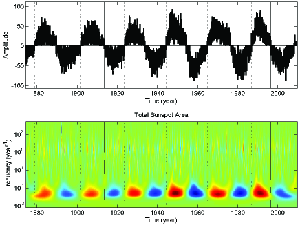
Figure 1.— Daily sunspot area time series: (a) The sunspot area time series in a Bracewell representation. This time series is proportional to the magnetic field (see text). (b) Wavelet transform of the daily sunspot area time series. Daily sunspot area data from 1874 to the present were compiled by NASA solar physics division. The vertical continuous and dotted lines define the dates of minimum of solar activity. The continuous lines are the beginning of a full magnetic cycle. The red and blue contour scales correspond to positive and negative variations of the magnetic field, respectively. The slight excess of intensity located at the right of each contour is a direct consequence of the difference between the rising and falling part of each demi-cycle. This legend applies to all the subsequent figures, unless stated otherwise.

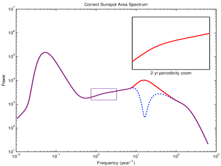
Figure 2.— Power spectral density of the sunspot area time series discussed in Figure 1. It is possible to identify two local maxima of intensity, occurring at two well-defined frequencies: one frequency with the value $f_{1}\sim 0.054\;{\rm year}^{-1}$, the well-known sunspot cycle with a period of $18.43$ yr, and a second frequency with the value $f_{2}\sim 16.11\;{\rm year}^{-1}$. This corresponds to a period of the order of $22.67\;{\rm day}$. The blue dotted line corresponds to the power spectral density of the sunspot area where the periodic source of $22.67\;{\rm day}$ was subtracted (see text).

The RGO has recorded sunspot areas using observational data from different observatories starting in 1874 until 1976. Following their work, the US Air Force (USAF) started compiling data from its own Solar Optical Observing Network, and more recently this work has been continued with the help of the US National Oceanic and Atmospheric Administration (NOAA), with much of the same information being organized and compiled until the present date. A complete reformatted data set has been made publicly available by the NASA/MSFC Solar Physics Division (Hathaway et al. 2002; Hathaway & Wilson 2004). The available records are the daily sunspot area data measurement made between 1874 May 1 and 2009 June 30. The sunspot areas were measured in units of millionths of a hemisphere. The three time series analyzed in this work have each a total of 49,370 data points each. The daily data time series correspond to a global sunspot area, the northern hemisphere sunspot area, and southern hemisphere sunspot area. In this analysis, we have assumed that the magnetic field reverse occurs in the solar minimum. We adopt the date of solar minimum activity, , the ones published in the publicly available data archives from US NOAA. For convenience, in this work we choose the most recent minimum to be 2008 January.

The procedure for the estimation of the magnitude of magnetic field $B(t)$ using sunspot areas is quite similar to the one used for sunspot numbers. It is worth noting that the correlation between the sunspot number and sunspot area is of $99\%$; therefore, there is no significant difference between these two proxies to estimate the intensity of the magnetic field (Hathaway & Wilson 2004). Since the magnetic field displays a period of approximately 22 yr with a polarity inversion every 11 yr, we will use the Bracewell number (Bracewell 1953) to explicitly take this feature into account. This quantity is defined as the square root of the sunspot area with a sign change at the beginning of each sunspot period. Therefore, each solar magnetic cycle will have one sunspot period with negative values and another with positive values. $B(t)$ can be computed as $B(t)=\beta_{A}\sqrt{A(t)}$, where $A(t)$ is the daily sunspot area measured. The parameter $\beta_{A}$ is a coefficient that converts the sunspot area proxy into the magnitude of the magnetic field. The studies of stability of tubes of magnetic flux suggest that the magnitude of the magnetic field inside the tachocline is between 1 and 10 T (Magara 2001; Lopes & Passos 2009). A comparative representation of the intensity of the magnetic field at the surface and the sunspot area allows us to estimate the conversion factor $\beta_{A}$ (Ringnes & Jensen 1960; Solanki 2003; Passos & Lopes 2008a). In this work we are interested in the variation of the mean magnetic field rather than its absolute value; therefore, without loss of generality, we choose $\beta_{B}$ to be equal to 1. In Figure 1 we present the wavelet transform of the global sunspot area. The power density spectrum is shown in Figure 2. It is possible to identify the long-term periodic solar magnetic field with a period 18.43 yr, among other features. A detailed analysis of Figure 2 also shows that in the frequency interval from $0.5\;{\rm year}^{-1}$ until $10\;{\rm year}^{-1}$, there are also other periodicities, like the biennial and Rieger periodicities. However, as the amplitudes of such periodicities are much less intense than the ones previously mentioned, these are not clearly visible on the spectrum, although a tiny sinusoidal feature is visible in the mentioned region. A discussion of the known periodic phenomena observed on the sunspot data series, with periods varying from several months to several years, can be found in Krivova & Solanki (2002).

To check the validity of the density power spectrum shown in Figure 2, we have computed this using another type of wavelet. Interestingly, the general form of the density power spectrum was also found using the Morlet/Gabor wavelet. Equally, for this wavelet the leading periodicities have the same proportionality relation between their amplitudes, a property consistent with the density power spectrum of the Mexican hat wavelet.

In the following section, we propose a theoretical model to interpret the obtained density spectrum.

5. Model of the stochastic nature of sunspot areas

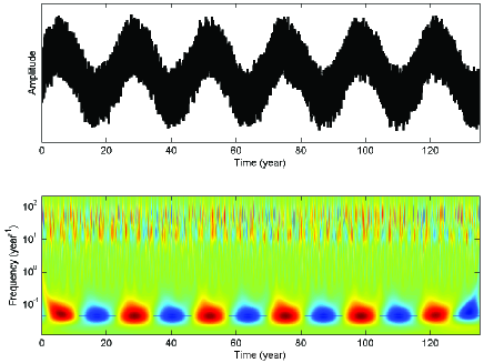
Figure 3.— Daily artificial data of the solar magnetic field $B(t)$. It is accepted that $B(t)$ has two components (see text for details): $B_{o}(t)$, a long-term scale variation (Van der Pol-Duffing oscillator solution), and $B_{c}(t)$, a short-term scale variation (random uniform noise and wave-like perturbation). (a) Six solar magnetic cycles time series of a noise cyclical-like curve. (b) Contour plot of ${\cal W}(\tau,f)$ for the noise cyclical- like curve in (a).

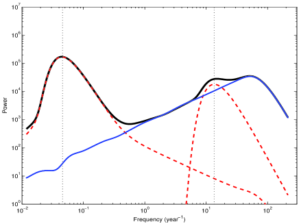
Figure 4.— Power spectral density of the noise cyclical-like curve discussed in Figure 1. The vertical lines indicate the location of $f_{o}=\omega_{o}/2\pi$ (left line) and $f_{p}=\omega_{p}/2\pi$ (right line). This corresponds to the values 21.87 yr ($f_{o}\sim 0.04572\;{\rm yr}^{-1}$) and 27 days ($f_{p}\sim 13.52\;{\rm yr}^{-1}$). The black curve corresponds to the full solution given by equation (2). The blue curve corresponds to the random stochastic source (see text). The dashed red curves correspond to the two single periodic sources with frequencies $f_{o}$ and $f_{p}$.

The daily temporal evolution of the $B(t)$ on the Sun’s surface can be interpreted as the final result of several physical mechanisms acting simultaneously on the continuous regeneration of the magnetic field. These magnetic field variations can be assumed to be constituted by two terms: one related to the long-term evolution of the solar magnetic cycle, as predicted by standard dynamo models, and a short-term component related to the excitation provided by the Sun’s surface granulation and short-term periodic flows. The turbulent flows preceding the formation of granules are not taken fully into account on the current solar dynamo models. Therefore, the observed magnetic field on the Sun’s surface, $B(t)$, will be the result of the superposition of these two distinct physical processes:

$$B(t)=B_{o}(t)+B_{c}(t),$$ (3)

where $B_{o}(t)$ and $B_{c}(t)$ are the long-term and the short-term components of evolution of the observed surface magnetic field, respectively. The component $B_{o}(t)$ is the long-term component of the magnetic field that is produced by the solar dynamo typically during a 22 yr period, and $B_{c}(t)$ is the short-term component of the magnetic field associated to the solar granulation and other short-term flows.

The evolution of the averaged magnetic field is described by a set of MHD equations in a simplified form, known as the axisymmetric dynamo model (Charbonneau 2010). It has been shown that $B_{o}(t)$ corresponds to the temporal part of the toroidal component of the averaged magnetic field (Mininni et al. 2001; Passos & Lopes 2008b). This axisymmetric formulation of the solar dynamo takes into account the contribution of the differential rotation and the meridional circulation flow. $B_{o}(t)$, which emerges at the solar surface, is the solution of a Van der Pol-Duffing oscillator(Lopes & Passos 2009),

$$\frac{d^{2}B_{o}}{dt}+\omega_{o}^{2}B_{o}+\mu\left(3\xi B_{o}^{2}-1\right)\frac{dB_{o}}{dt}-\lambda B_{o}^{3}=0,$$ (4)

where the coefficients $\omega_{o}$, $\mu$, $\xi$, and $\lambda$ are averages of the solar background used in the solar dynamo model. These quantities can be estimated from the observational data(Passos & Lopes 2008a, b). Following our previous work and in agreement with what is published in the literature, we adopt the following set of averaged values for our numerical simulations(Lopes & Passos 2009): $\omega_{o}=0.2873$, $\mu=0.1556$, $\xi=0.0221$, and $\lambda=1.5\times 10^{-4}$. In the numerical simulation $B_{o}(t)$ takes values between -100 and +100 in arbitrary units. The value of $\omega_{o}=2\pi f_{o}=0.2873$ corresponds to a magnetic cycle of a 22 yr period (i.e., a linear frequency $0.0457{\rm yr}^{-1}$). This long-term periodicity is responsible for the strongest periodic source in the density power spectrum of the sunspot area data (see Figure 2).

The short-term component, $B_{c}(t)$, emulates the stochastic excitation provided by small-scale flows, possibly like the solar granulation, including additional periodic flows (not included on the solar dynamo model), very likely related with the local hydrodynamics. The turbulent flows of the convection zone produce a complex pattern of structure observed on the Sun’s surface. These motions seem to be arranging in hierarchy of surface outflows, which are the manifestations of the convective fluid motions below the photosphere. Usually these structures are characterized as patterns of granulations, meso-granulations and super-granulations. These well-defined granulation structures have typical scales of $1$, $10$ and $15-35$ Mm and averaged lifetimes of the $0.2$, $5$ and $24$ h, respectively. The daily variability observed in sunspot areas is very likely connected with the complex processes related with local flows and the chaotic motion of the short-scale magnetic fields associated with these granules. This random magnetic behavior is very likely responsible for the stochastic nature of sunspot area data (see Figure 2). Therefore, we choose $B_{c}(t)$ to be a stochastic source, ${\cal A}_{r}U(t)$, where ${\cal A}_{r}$ is the amplitude of a stochastic excitation source and $U(t)$ is a uniform distribution that takes values between -1 and 1.

Another source term that is identified in the sunspot area data is a periodic source, the second strongest peak, located at a higher frequency (see Figure 2). There is the possibility that some of the periodic flows produced inside the star could present such a type of signature in the power spectrum. Unfortunately, other well-known processes could produce a similar structure. One of our concerns relates to the possibility that such a periodic source is related to the synodic rotation, , or Carrington rotation, assumed to be of the order of 27 days. Equally, Sturrock & Bai (1992) have identified a sunspot feature with a period of 26 days.

One of our concerns in the analysis of observational density power spectrum is to identify the origin of the 22.67 day periodicity. Therefore, we choose to study the contribution of such a term to the power spectrum. Nevertheless, regardless of the origin of this periodic source on the data, either being caused by the Carrington rotation or the 26 day periodicity  Sturrock & Bai (1992), or possibly produced by some other mechanism inside the star, we will study how the density power spectrum is modified by the presence of such a periodic source. Accordingly, we choose our theoretical periodic phenomena as a fiducial period of 27 days. It follows that the second term of $B_{c}(t)$ is a periodic function with amplitude ${\cal A}_{p}$ and cyclic frequency $\omega_{p}$, hence, ${\cal A}_{p}\sin{(\omega_{p}t)}$. Hence,

$$B_{c}(t)={\cal A}_{r}U(t)+{\cal A}_{p}\sin{(\omega_{p}t)}.$$ (5)

There are other periodicities in the observational density spectrum. However, as these quantities have an amplitude much smaller than the one previously mentioned and the 22 yr solar cycle, they are not considered in this preliminary study.

Figure 3(a) shows the $B(t)$ times series obtained for a simulation with the following fiducial values: ${\cal A}_{r}=100$ and ${\cal A}_{p}=30$ in arbitrary units. The period of this source term is of 27 days, i.e., $\omega_{p}=85$.

The two-dimensional wavelet transform ${\cal W}(\tau,f)$ of the artificial data time series $B(t)$ is shown in Figure 3b. The oscillation pattern around $f\sim 10^{-1}\;{\rm year}$ is the distinct signature of the solar dynamo, i. e., $f_{o}=\omega_{o}/2\pi$. A careful analysis of Figure 3b shows the second periodic signal near $10^{2}\;{\rm year}^{-1}$, i.e., $f_{p}=\omega_{p}/2\pi$.

In Figure 4, we shown the power spectrum of the artificial time series $B(t)$ computed previously (see Figure 3). The maximum of intensity for ${\cal W}(\tau,f)$ and $P(f)$ occurs for values of $B(t)$, that have a cyclic behavior, namely, the two cyclic frequencies: $\omega_{o}$ and $\omega_{p}$. The random behavior of the time series, which we attribute to the stochastic nature of the sunspot areas, is shown in this power spectrum as a continuum, rather than the usual random noise observed in the Fourier spectrum. The presence of a stochastic source term ${\cal A}_{r}U(t)$ increases significantly the power of the spectrum at high frequencies. More significantly, the amplitude power of the second cyclic source, ${\cal A}_{p}\sin{(\omega_{p}t)}$ increases with the magnitude of the stochastic source, but it is still possible to identify the location of the maximum for this source term (compare the two curves in the power spectrum). The three source terms of the artificial time series are clearly identified in the power spectrum (see Figure 3).

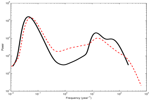
Figure 5.— Wavelet transform of the daily sunspot area time series. Comparison between the spectra of the total sunspot area observed data and the sunspot proposed model. The black curve is computed for the theoretical model with two periodic functions, the periods of 21.87 year and 27 days. The dashed red line corresponds to the sunspot data, where local maximums occur for the periods $18.43\;{\rm yr}$ and $22.67\;{\rm days}$.

6. Discussion

The daily time series displays the inherent noisiness of the solar cycle, very likely related to the turbulent flows of the Sun’s surface. The data series changes widely daily. The Sun rotates with a period of 25 days (at the equator), during which the solar activity can change significantly, which corresponds to a synodic rotation period of 26.24 days, although the Carrington rotation is assumed to be of the order of 27 days. Earth observers can only measure sunspots from the observed hemisphere. To compensate this fact, the usual procedure is to use some kind of temporal filter to smooth the data, typically a 13-month running mean. This procedure strongly reduces the stochastic noise at high frequencies. Unfortunately, this procedure also removes the contribution of perturbations to the sunspot cycle, with high frequencies. By using the wavelet procedure previously introduced, we have analyzed the time series over all the entire range of frequencies allowed. Using the proposed technique, there is no need for mean averages, once the full time series can be completely reproduced (in the mathematical sense) as a sum of basic time series at different scales (in our case, frequencies). Each scale is somehow an average of the observational time series at that scale. More importantly, the small scales are maintained on the series. In fact, the study of small scale processes in the Sun can be done by this method, once we can assume that the physical processes occurring at a small-scale, which are measured in the observed hemisphere, also occur in other parts of the Sun. The weakness of such a procedure is that. in principle, a periodicity related to the Carrington rotation should appear, if not cancelled out by some average behavior. We believe that the total daily areas of the observed Sun’s globe or each of its hemispheres, on average, are not affected by the Carrington rotation period, once this contribution in average cancels out.

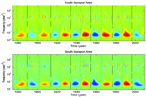
Figure 6.— Wavelet transform of the daily sunspot area time series of the northern and southern hemisphere. In both hemispheres we find the same typical behavior, namely, the existence of an excess of energy near a frequency of the order of $10^{2}\;{\rm year^{-1}}$. For both hemispheres, it is possible to identify a small excess of intensity for lower frequencies.

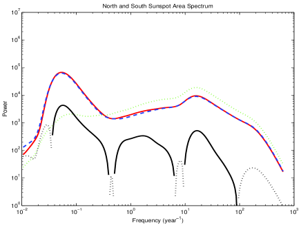
Figure 7.— Power spectral density of the sunspot area time series of the northern and southern hemispheres as discussed in Figure 6. The continuous red curve corresponds to the power spectral density of the northern hemisphere and the dashed blue curve to power spectral density of the southern hemisphere. The continuous-dotted black curve shows the spectral regions where the northern hemisphere is more active than the southern hemisphere (continuous) or the reverse (dotted line). The dotted green line corresponds to the power spectral density computed from wavelet intensity differences between the two hemispheres. The first peak ($f_{1}$) shows a strong correlation between hemispheres, whereas the second peak ($f_{2}$) shows no correlation at all between the two hemispheres.

6.1. The global sunspot area

The plot of the magnetic field computed from the global sunspot area is shown in Figure 1, and the power spectrum is shown in Figure 2. We distinguish three distinct components related to the solar magnetic field: one spectral peak produced by an excess of power is located near $f_{1}\sim 0.054\;{\rm year}^{1}$, a second spectral peak is located near $f_{2}\sim 16.11\;{\rm year^{-1}}$, and a third component is the increase of power toward the high frequencies, which we associated with the daily turbulent excitation of sunspots.

The forms of these components are similar to the ones discussed in the artificial data time series (see Figures 3 and 4). In Figure 5 we compare the theoretical model computed (discussed in the previous section) with the observed power spectrum. The first striking result is the similarity between the two curves.

The strongest excess of power occurs for the frequency $f_{1}\sim 0.054\;{\rm yr}^{-1}$, or 18.42-year period. Although the source is cyclic, it presents quite substantial intensity variations from cycle to cycle. The contour plot of ${\cal W}(\tau,f)$ is asymmetric, presenting an excess of intensity on the right side, similar to the theoretical model previously discussed. The second excess of power of the time series is located at a frequency of $16.11\;{\rm year^{-1}}$ which corresponds to an apparent period of 22.67 days. It is worth mentioning that such a secondary peak on the power density spectrum has an intensity value only 15% smaller than the main peak associated with the 22 yr solar magnetic cycle. It seems to be a quite strong source. In Figure 2 we show the shown the case where this last periodic term is removed and the overall spectrum maintains the same structure.

We have made other analyses of these time series, namely, we have computed the power spectrum from the original sunspot area data time series, without the introduction of the Bracewell numbers, and we have found the same excess of power in the same locations of the power spectrum. Once again, this is observed in all the three time series, observed Sun’s disk, northern hemisphere, and southern hemisphere. These results confirm our initial hypothesis that there is an oscillation component of 22.67 days on the sunspot time series.

However, establishing the exact physical origin of such periodic source is more difficult. It could be related to the Carrington rotation, the 26 day periodicity found by Sturrock & Bai (1992), or it could have originated in the interior of the Sun. Nevertheless, the 22.67 day period is quite different from these other two periodicities. To investigate the origin of such a secondary source, we have made a spectral analysis of each of the solar magnetic cycles. We found that the secondary source peaks in each of the solar magnetic cycles continues to exist, but the period takes values between 21.5 and 24 days. These values occur between different solar magnetic cycles, but also between different hemispheres, even if values near 22.67 days occur with more frequency. This is the stronger indicator that suggests that the origin of such a secondary source is related to physical processes inside the Sun. Actually, there are several internal flows that operate in similar timescales. The internal rotation and additional averaged flows could be at the origin of the formation of observed sunspot patterns (Wolff 1995; Gizon et al. 2003b, a; Howe et al. 2006). The available data do not allow us to test further the hypothesis that this power access at high frequency have originated by the Carrington rotation. Finally, it is possible to identify an almost linear increase of power between frequencies $0.5\;{\rm yr^{-1}}$ and $5\;{\rm yr^{-1}}$ . This very likely is related to turbulent noise of granulation. This stochastic noise is present all over the spectrum, but it is more noticeable in the mentioned frequency interval (see Figure 2). In Figure 5 the similarity of behaviors between the theoretical model and observation is very clear, although there is scope for improvement.

6.2. The North and South sunspot area time series

The comparative analyses of the power spectrum for both hemispheres (see Figures 6 and 7) show very similar results. There is an indication of an asymmetric behavior between the northern and the southern hemisphere. For very low frequencies ($f\leq 310^{-2}\;{\rm yr}^{-1}$), the southern hemisphere seems to present an excess of energy when compared with the northern hemisphere (see Figure 7), as has been reported in previous works(Hathaway & Wilson 2004; Donner & Thiel 2007). Several authors have found evidence of this asymmetry for different proxies at distinct timescales (e.g., Valdés-Galicia et al. 1996; Valdés-Galicia & Velasco 2008; Li et al. 2009; Chowdhury et al. 2013). However, for larger frequencies ($f\geq 310^{-2}\;{\rm yr}^{-1}$) the situation is quite the reverse: the northern hemisphere seems to present an excess of energy in relation to the southern hemisphere. In this spectral interval, we found three strong excitation sources, which present quite different characteristics. There is a systematic excess of power for the northern hemisphere when compared with the southern hemisphere, namely, near the two studied periodic sources, as well as in the intermediate region where the biennial and Rieger periodicities are known to be located. This is also the region of the spectrum where the turbulent processes of the convection zone seem to make the most important contribution for the dynamics of sunspots.

The source related with the 18.42 yr period associated with the long-term solar magnetic cycle is strongly correlated between the two hemispheres, although the source located at a period of 22.67 days is not correlated (see Figure 7). This is clearly illustrated by computing the power spectral density of the difference between the two hemispheres, where for the low frequency the effects cancel out, and for the high frequency they add up, i.e., the 18.42 yr period physical process is strongly correlated, but the 22.67 day period seems to be equally independent of each hemisphere. This suggests that the 22.67 day periodicity has a phenomena strongly asymmetric between the two hemispheres. Moreover, as per Figure 7, the physical process is more pronounced in the northern hemisphere.

6.3. Comparison with Lomb-Scargle spectral analysis

We complement the wavelet study of the total sunspot area with a Lomb-Scargle (LS) spectral analysis. This technique was developed for interrupted data sets in astrophysics (Lomb 1976; Scargle 1982) and is often used to do spectral studies in different sciences. Actually, the total daily area of sunspots is an uneven time series because of the days when there were no observations (represented in the data sets as -1). LS spectra provide the significant frequencies (in a statistical sense) and their respective amplitudes, enabling a proper evaluation of the dominant periods that influence the data. The program used in the present study is an LS implementation (Press et al. 1992).

The parameters used are hifac = 1 (which defines the frequency limit as hifac times the average Nyquist frequency) and ofac = 4 (oversampling factor). Moreover, to verify the statistical significance of the 22.67 day period found above, we calculated the LS spectrum for half-year range from 1875 until 2013 (this means 276 LS spectra). From them we select the significant periods in the range of 20–30 days; some half-years do not have periods in this range, the majority have one, others have two significant periods, and only one has three. In Figure 8, the upper panel shows the LS periodogram for the first half of 1890, where the 22.67 day period is really clear. The lower panel represents the values of the significant periods found in a histogram. It is important to mention that in a half-year it is possible to have six to eight complete cycles with periods in the range of 20-30 days, enough to be detected if present. Two peaks dominate the histogram: one for periods between 22 nd 23 days with 41 occurrences, the other for periods between 26 and 27 days having 43 counts. This is significant because the first peak corresponds to the 22.67 day periodicity. The second peak corresponds to either the Carrington rotation of the 25.8 days periodicity found by (Sturrock & Bai 1992), although the second interpretation seems to be more reliable. The clear identification of such periodicity clearly shows that the first periodicity is distinct from the second one.

To clarify the dependency of the significant periods on the evolution of the sunspot area, we calculate the mean value of the sunspot area for every half-year similarly to what he have done for the LS periodograms. After that, we plot the distribution of the significant periods in the 20–30 day range as a function of the half-year mean sunspot area using an efficient 2D histogram, Figure 9. The dominance of the periods in the range of 22–23 days and 26–27 days is clear; this is consistent with the 1D histogram (see Figure 8). Naturally, there are fewer counts for higher sunspot areas; this is because the occurrence of sunspot areas is progressively decreases as the areas increase, and not because they do not generate periodicities in the range of interest. Moreover, the occurrence of periods in these two ranges seems not to be dependent on the sunspot area. Even though no direct relation exists between the 22 and 23 day periodicities and the solar cycle strength, there is some indication of a possible connection. To illustrate this point, we represent the power of the significant periods in the range of 22–23 days along with the sunspot area from 1874 until 2013. Figure 10 shows that power clusters around two distinct levels, one around 28 and another around 80. It is clear that the power of $\sim$80 became more frequent after 1930, and this could be tentatively attributed to the onset of the modern maximum from 1950 up to 2000.

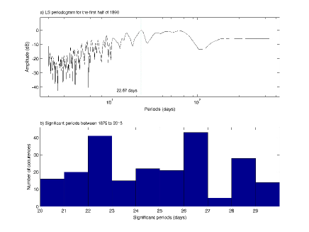
Figure 8.— Upper panel: representative LS periodogram for the first half of 1890. Lower panel: histogram of the significant frequencies in the 20–30 days range. The histogram shows two periodicities located at 22.67 and 26.6 days (see main text).

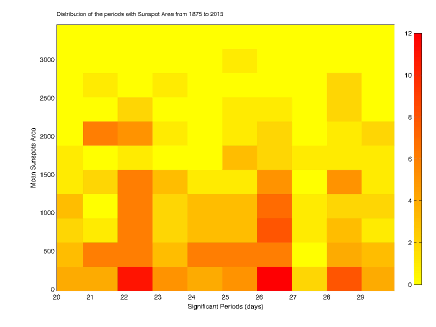
Figure 9.— Periodicity relations with the sunspot areas: 2D histogram distribution of periods in the 20–30 day range as a function of the half-year mean sunspot areas.

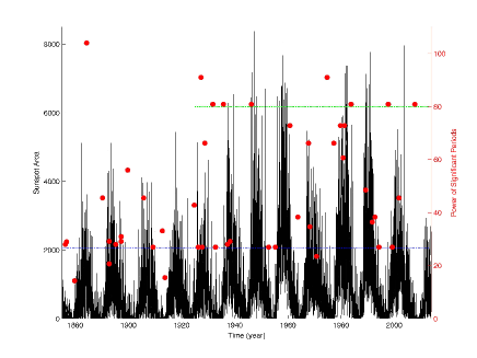
Figure 10.— Horizontal lines define the two typical power scales: one around 28 (marked as a blue dotted line) and another around 80 (marked as a green dotted line).

7. Conclusion

In this work, we made a spectral analysis of the daily sunspot areas, to identify the different mechanisms underlying the evolution of the magnetic field, or to be more exact regarding the dynamics of the surface’s magnetic field. Our study of the sunspot area time series, revealed clear signatures pointing to the possibility that the global behavior of the solar magnetic cycle is affected by different physical processes.

The leading result of this work is found in Figure 5, where we compare the power spectral density of the theoretical model with the equivalent spectrum computed from daily time series of sunspot areas. In both spectra it is possible to identify three well-defined structures: two major periodic sources located at 18 yr and 23 days and a spectral continuum in the power spectral density, clearly visible between these two leading periodicities. In between these periodicities, the intensity of the spectral continuum increases as the frequency decreases. Moreover, the spectral line widths of the peaks corresponding to the 18 yr and 23 days periodic phenomena somehow measure the variability of the periods of such phenomena during the duration of the time series.

The 18 yr periodicity is the well-known self-regulated mechanism of the dynamo that converts kinetic energy into magnetic energy and is responsible for the 22 yr solar magnetic activity, which we estimate to be of the order of 18.42 yr. The second term seems to be intrinsically of stochastic nature, possibly associated with the turbulent processes of the convective region and granulation. Finally, this method of analysis also reveals another contributor to the evolution of the magnetic field: a cycle source with a period of 22.67 days.

An important result of this study is the identification of the spectral continuum in the sunspot area time series, mostly visible as a linear continuum between the 18 yr and 23 day periodic sources. This continuum is a signature of the contribution of granulation and turbulent convection for the variability of the sunspot areas. It is worth recording that the magnetic field on the solar surface displays a systematic pattern of activity that is mapped by sunspot numbers and areas. These sunspots are produced by localized concentration of magnetic fields with intensities of the order of a kilogauss. As the sunspots inhibit the convection in the Sun, they change significantly the global behavior of turbulence and magnetism in the solar convection zone. In particular, as the intensity of the magnetic field within a nearly formed sunspot decreases with time, the impact of granulation on the sunspot area becomes more relevant. Accordingly, by measuring the random behavior of sunspot areas over time, we are obtaining information about the impact of granulation on the evolution of the magnetic field.

Finally, we have been able to reproduce most of the results found in the observational data by using a simple solar oscillator model. We have found that an oscillator model with a periodic source of 27 days (which could be either be the Carrington rotation or the 26 days periodicity Sturrock & Bai (1992)) presents a very similar structure to the one found in the observed power density spectrum. Nevertheless, the value determined from observational data, i.e. 22.67 days, is quite different from these two periodicities. Moreover, we have made an independent LS spectral analysis of the sunspot data and have confirmed that the 22.67 day periodicity is distinct from the two others previously mentioned. Nevertheless, we found that this periodicity is located near other periodicities. There is the strong possibility that such specific periodic structure is produced by some unknown internal process inside the convection zone. The analysis of this source term in each of the hemispheres indicates that term has a very identical nature in both hemispheres, i.e., there is no correlation between the two hemispheres. This is quite different from the 18.42 yr periodic term, which has strong correlation between the hemispheres. The asymmetry between hemispheres is stronger for the higher frequencies, especially near the two periodic sources.

References

- Benevolenskaya (1998) Benevolenskaya, E. E. 1998, ApJ, 509, L49
- Berdyugina & Usoskin (2004) Berdyugina, S. B., & Usoskin, I. G. 2004, in IAU Symposium ”Stars as Suns : Activity, Evolution and Planets”, ed. A. K. Dupree & A. O. Benz, IAU Symposium, Vol. 219, 128
- Bracewell (1953) Bracewell, R. N. 1953, Nature, 171, 649
- Charbonneau (2005) Charbonneau, P. 2005, Living Reviews in Solar Physics, 2, 2
- Charbonneau (2010) —. 2010, Living Reviews in Solar Physics, 7, 3
- Chowdhury et al. (2013) Chowdhury, P., Choudhary, D. P., & Gosain, S. 2013, ApJ, 768, 188
- Corbard & Thompson (2002) Corbard, T., & Thompson, M. J. 2002, Sol. Phys., 205, 211
- Dikpati & Charbonneau (1999) Dikpati, M., & Charbonneau, P. 1999, ApJ, 518, 508
- Dikpati & Gilman (2006) Dikpati, M., & Gilman, P. A. 2006, ApJ, 649, 498
- Donner & Thiel (2007) Donner, R., & Thiel, M. 2007, A&A, 475, L33
- Duvall (1980) Duvall, Jr., T. L. 1980, Sol. Phys., 66, 213
- Fröhlich & Lean (2004) Fröhlich, C., & Lean, J. 2004, A&A Rev., 12, 273
- Gizon et al. (2003a) Gizon, L., Duvall, T. L., & Schou, J. 2003a, Nature, 421, 764
- Gizon et al. (2003b) —. 2003b, Nature, 421, 43
- Gough & McIntyre (1998) Gough, D. O., & McIntyre, M. E. 1998, Nature, 394, 755
- Guerrero et al. (2009) Guerrero, G., Dikpati, M., & de Gouveia Dal Pino, E. M. 2009, ApJ, 701, 725
- Hathaway (2010) Hathaway, D. H. 2010, Living Reviews in Solar Physics, 7, 1
- Hathaway et al. (2010) Hathaway, D. H., Williams, P. E., Dela Rosa, K., & Cuntz, M. 2010, ApJ, 725, 1082
- Hathaway & Wilson (2004) Hathaway, D. H., & Wilson, R. M. 2004, Sol. Phys., 224, 5
- Hathaway et al. (2002) Hathaway, D. H., Wilson, R. M., & Reichmann, E. J. 2002, Sol. Phys., 211, 357
- Howard & Labonte (1980) Howard, R., & Labonte, B. J. 1980, ApJ, 239, L33
- Howe (2009) Howe, R. 2009, Living Reviews in Solar Physics, 6, 1
- Howe et al. (2005) Howe, R., Christensen-Dalsgaard, J., Hill, F., et al. 2005, ApJ, 634, 1405
- Howe et al. (2006) Howe, R., Komm, R., Hill, F., et al. 2006, Sol. Phys., 235, 1
- Jiang et al. (2007) Jiang, J., Chatterjee, P., & Choudhuri, A. R. 2007, MNRAS, 381, 1527
- Krivodubskij (2010) Krivodubskij, V. 2010, in COSPAR Meeting, Held 18-15 July 2010, in Bremen, Germany, p.2 COSPAR Meeting, Vol. 38, 8th COSPAR Scientific Assembly, 1770
- Krivova & Solanki (2002) Krivova, N. A., & Solanki, S. K. 2002, A&A, 394, 701
- Li et al. (2009) Li, K. J., Gao, P. X., & Zhan, L. S. 2009, Sol. Phys., 255, 289
- Lomb (1976) Lomb, N. 1976, Astrophysics and Space Science, 39, 447
- Lopes & Passos (2009) Lopes, I., & Passos, D. 2009, MNRAS, 397, 320
- Lopes et al. (2014) Lopes, I., Passos, D., Nagy, M., & Petrovay, K. 2014, Space Science Volume 186, Issue 1-4, pp. 535-559
- Lou et al. (2003) Lou, Y.-Q., Wang, Y.-M., Fan, Z., Wang, S., & Wang, J. X. 2003, MNRAS, 345, 809
- Magara (2001) Magara, T. 2001, ApJ, 549, 608
- Mallat (1997) Mallat, S. 1997, A Wavelet Tour of Signal Processing (London: AP Professional)
- Miesch & Toomre (2009) Miesch, M. S., & Toomre, J. 2009, Annual Review of Fluid Mechanics, 41, 317
- Mininni et al. (2001) Mininni, P. D., Gomez, D. O., & Mindlin, G. B. 2001, Sol. Phys., 201, 203
- Moffatt (1978) Moffatt, H. K. 1978, Magnetic field generation in electrically conducting fluids,Cambridge University Press, 1978. 353 p.
- Muñoz-Jaramillo et al. (2009) Muñoz-Jaramillo, A., Nandy, D., & Martens, P. C. H. 2009, ApJ, 698, 461
- Parker (1955) Parker, E. N. 1955, ApJ, 122, 293
- Passos & Lopes (2008a) Passos, D., & Lopes, I. 2008a, ApJ, 686, 1420
- Passos & Lopes (2008b) —. 2008b, Sol. Phys., 250, 403
- Petrovay (2010) Petrovay, K. 2010, Living Reviews in Solar Physics, 7, 6
- Petrovay & Christensen (2010) Petrovay, K., & Christensen, U. R. 2010, Space Sci. Rev., 155, 371
- Pipin & Kosovichev (2014) Pipin, V. V., & Kosovichev, A. G. 2014, ApJ, 785, 49
- Press et al. (1992) Press, W. H., Teukolsky, S. A., Vetterling, W. T., & Flannery, B. P. 1992, Numerical recipes in C. The art of scientific computing
- Rempel & Cheung (2014) Rempel, M., & Cheung, M. C. M. 2014, ApJ, 785, 90
- Rieger et al. (1984) Rieger, E., Kanbach, G., Reppin, C., et al. 1984, Nature, 312, 623
- Ringnes & Jensen (1960) Ringnes, T. S., & Jensen, E. 1960, Astrophysica Norvegica, 7, 99
- Scargle (1982) Scargle, J. 1982, ApJ, 263, 835
- Schou et al. (2002) Schou, J., Howe, R., Basu, S., et al. 2002, ApJ, 567, 1234
- Shibahashi (2007) Shibahashi, H. 2007, Astronomische Nachrichten, 328, 264
- Simoniello et al. (2013) Simoniello, R., Jain, K., Tripathy, S. C., et al. 2013, ApJ, 765, 100
- Solanki (2003) Solanki, S. K. 2003, A&A Rev., 11, 153
- Solanki et al. (2013) Solanki, S. K., Krivova, N. A., & Haigh, J. D. 2013, ARA&A, 51, 311
- Sturrock & Bai (1992) Sturrock, P. A., & Bai, T. 1992, ApJ, 397, 337
- Tobias (1997) Tobias, S. M. 1997, A&A, 322, 1007
- Valdés-Galicia et al. (1996) Valdés-Galicia, J. F., Pérez-Enríquez, R., & Otaola, J. A. 1996, Sol. Phys., 167, 409
- Valdés-Galicia & Velasco (2008) Valdés-Galicia, J. F., & Velasco, V. M. 2008, Advances in Space Research, 41, 297
- Vorontsov et al. (2002) Vorontsov, S. V., Christensen-Dalsgaard, J., Schou, J., Strakhov, V. N., & Thompson, M. J. 2002, Science, 296, 101
- Wolff (1995) Wolff, C. 1995, ApJ, 443, 423
- Zaqarashvili et al. (2010) Zaqarashvili, T. V., Carbonell, M., Oliver, R., & Ballester, J. L. 2010, ApJ, 709, 749
- Zhao et al. (2013) Zhao, J., Bogart, R. S., Kosovichev, A. G., Duvall, Jr., T. L., & Hartlep, T. 2013, ApJ, 774, L29
- Zhao & Kosovichev (2004) Zhao, J., & Kosovichev, A. G. 2004, ApJ, 603, 776