Fundamental limits of remote estimation of autoregressive Markov processes under communication constraints

Abstract

The fundamental limits of remote estimation of autoregressive Markov processes under communication constraints are presented. The remote estimation system consists of a sensor and an estimator. The sensor observes a discrete-time autoregressive Markov process driven by a symmetric and unimodal innovations process. At each time, the sensor either transmits the current state of the Markov process or does not transmit at all. The estimator estimates the Markov process based on the transmitted observations. In such a system, there is a trade-off between communication cost and estimation accuracy. Two fundamental limits of this trade-off are characterized for infinite horizon discounted cost and average cost setups. First, when each transmission is costly, we characterize the minimum achievable cost of communication plus estimation error. Second, when there is a constraint on the average number of transmissions, we characterize the minimum achievable estimation error. Transmission and estimation strategies that achieve these fundamental limits are also identified.

I Introduction

I-A Motivation and literature overview

In many applications such as networked control systems, sensor and surveillance networks, and transportation networks, etc., data must be transmitted sequentially from one node to another under a strict delay deadline. In many of such real-time communication systems, the transmitter is a battery powered device that transmits over a wireless packet-switched network; the cost of switching on the radio and transmitting a packet is significantly more important than the size of the data packet. Therefore, the transmitter does not transmit all the time; but when it does transmit, the transmitted packet is as big as needed to communicate the current source realization. In this paper, we characterize fundamental trade-offs between the estimation error (or distortion) and the cost or average number of transmissions in such systems.

In particular, we consider a sensor that observes a first-order autoregressive Markov process. At each time instant, based on the current state of the process and the history of its past decisions, the sensor determines whether or not to transmit the current state. If the sensor does not transmit, the receiver must estimate the state using the previously transmitted values. A per-step distortion function measures the estimation error. We investigate two fundamental trade-offs in this setup: (i) when there is a cost associated with each communication, what is the minimum expected estimation error plus communication cost; and (ii) when there is a constraint on the average number of transmissions, what is the minimum estimation error. For both these cases, we characterize the transmission and estimation strategies that achieve the optimal trade-off.

Two approaches have been used in the literature to investigate real-time or zero-delay communication. The first approach considers coding of individual sequences [1, 2, 3, 4]; the second approach considers coding of Markov sources [5, 6, 7, 8, 9, 10]. The model presented above fits with the latter approach. In particular, it may be viewed as real-time transmission, which is noiseless but expensive. In most of the results in the literature, the focus has been on identifying sufficient statistics (or information states) at the transmitter and the receiver; for some of the models, a dynamic programming decomposition has also been derived. However, very little is known about the solution of these dynamic programs.

The communication system described above is much simpler than the general real-time communication setup due to the following feature: whenever the transmitter transmits, it sends the current state to the receiver. These transmitted events reset the estimation error to zero. We exploit these special features to identify an analytic solution to the dynamic program corresponding to the above communication system.

A static (one shot) remote estimation problem was first considered in [11] in the context of information gathering in organizations. The problem of optimal off line choice of measurement times was considered in [12], whereas the problem of optimal online choice of measurement times was considered in [13]. The closely related problem of event-based sampling (also called Lebesgue sampling) was considered in [14]. In addition, several variations of the remote estimation problem have been considered in the literature. The most closely related models are [15, 16, 17, 18, 1, 20], which are summarized below. Other related work includes censoring sensors [21, 22] (where a sensor takes a measurement and decides whether to transmit it or not; in the context of sequential hypothesis testing), estimation with measurement cost [23, 24, 25] (where the receiver decides when the sensor should transmit), sensor sleep scheduling [26, 27, 28, 29] (where the sensor is allowed to sleep for a pre-specified amount of time); and event-based communication [30, 32, 31] (where the sensor transmits when a certain event takes place). We contrast our model with [18, 1, 20] below.

In [15], optimal remote estimation of i.i.d. Gaussian processes is investigated under a constraint on the total number of transmissions. The optimal estimation strategy is derived when the transmitter is restricted to be of threshold-type.

In [16], the optimal remote estimation of a continuous-time autoregressive Markov process driven by Brownian motion is considered under a constraint on the number of transmissions. The optimal transmission strategy is derived under an assumption on the structure of the optimal estimation strategy. It is shown that the optimal transmission strategy is of a threshold-type, where the thresholds are determined by solving a sequence of nested optimal stopping problems.

In [17] optimal remote estimation of Gauss-Markov processes is investigated when there is a cost associated with each transmission. The optimal transmission strategy is derived when the estimation strategy is restricted to be Kalman-like.

In [18, 1, 20], optimal remote estimation of autoregressive Markov processes is investigated when there is a cost associated with each transmission. It is assumed that the autoregressive process is driven by a symmetric and unimodal noise process but no assumption is imposed on the structure of the transmitter or the receiver. Using different solution approaches ( [18, 1] use majorization theory while [20] uses person-by-person optimality), it is shown that the optimal transmission strategy is threshold-based and the optimal estimation strategy is Kalman-like (the precise form of these strategies is stated in Theorem 8). Thus, the optimal transmission and estimation strategies are easy to implement.

An immediate question is how to identify the optimal transmission and estimation strategies for a given communication cost. It is shown in [18, 1, 20] that the optimal estimation strategy does not depend on the communication cost while the optimal transmission strategy can be computed by solving an appropriate dynamic program. However, the dynamic programs presented in [18, 1, 20] do not exploit the threshold structure of the optimal strategy.

In this paper, we provide an alternative approach to identify the optimal transmission strategies. We consider infinite horizon remote estimation problem and show that there is no loss of optimality in restricting attention to transmission strategies that use a time homogeneous threshold. To determine the optimal threshold, we first provide computable expressions for the performance of a generic threshold-based transmission strategy and then use these expressions to identify the best threshold-based strategy. Thus, we show that the structure of optimal strategies derived in [18, 1, 20] is also useful to compute the optimal strategy.

I-B Contributions

We investigate remote estimation for two models of Markov processes—discrete state autoregressive Markov processes (Model A) and continuous state autoregressive Markov processes (Model B); both driven by symmetric and unimodal innovations process—under two infinite horizon setups: the discounted setup with discount factor $\beta\in(0,1)$ and the long term average setup, which we denote by $\beta=1$ for uniformity of notation. For both models, we consider two fundamental trade-offs:

1. Costly communication: When each transmissions costs $\lambda$ units, what is the minimum achievable cost of communication plus estimation error, which we denote by $C^{*}_{\beta}(\lambda)$.

2. Constrained communication: When the average number of transmissions are constrained by $\alpha\in(0,1)$, what is the minimum achievable estimation error, which we denote by $D^{*}_{\beta}(\alpha)$ and refer to as the distortion-transmission trade-off.

We completely characterize both trade-offs. In particular,

• In Model A, $C^{*}_{\beta}(\lambda)$ is continuous, increasing, piecewise-linear, and concave in $\lambda$ while $D^{*}_{\beta}(\alpha)$ is continuous, decreasing, piecewise-linear, and convex in $\alpha$. We derive explicit expressions (in terms of simple matrix products) for the corner points of both these curves.

• In Model B, $C^{*}_{\beta}(\lambda)$ is continuous, increasing, and concave in $\lambda$ while $D^{*}_{\beta}(\alpha)$ is continuous, decreasing, and convex in $\alpha$. We derive an algorithmic procedure to compute these curves by using solutions of Fredholm integral equations of the second kind. When the innovations process is Gaussian, we characterize how these curves scale as a function of the variance $\sigma^{2}$.

We also explicitly identify transmission and estimation strategies that achieve any point on these trade-off curves. For all cases, we show that: (i) there is no loss of optimality in restricting attention to time-homogeneous strategies; (ii) the optimal estimation strategy is Kalman-like; (iii) the optimal transmission strategy is a randomized threshold-based strategy for Model A and is a deterministic threshold-based strategy for Model B.

In addition,

• In Model A, the optimal threshold as a function of $\lambda$ or $\alpha$ can be computed using a look-up table.

• In Model B, the optimal threshold as function of $\lambda$ or $\alpha$ can be computed using the solutions of Fredholm integral equations of the second kind.

I-C Notation

We use the following notation. $\mathds{Z}$, $\mathds{Z}_{\geq 0}$ and $\mathds{Z}_{>0}$ denote the set of integers, the set of non-negative integers and the set of strictly positive integers, respectively. Similarly, $\mathds{R}$, $\mathds{R}_{\geq 0}$ and $\mathds{R}_{>0}$ denote the set of reals, the set of non-negative reals and the set of strictly positive reals, respectively. Upper-case letters (e.g., $X$, $Y$) denote random variables; corresponding lower-case letters (e.g. $x$, $y$) denote their realizations. $X_{1:t}$ is a short hand notation for the vector $(X_{1},\dots,X_{t})$. Given a matrix $A$, $A_{ij}$ denotes its $(i,j)$-th element, $A_{i}$ denotes its $i$-th row, $A^{\intercal}$ denotes its transpose. We index the matrices by sets of the form $\{-k,\dots,k\}$; so the indices take both positive and negative values. For $k\in\mathds{Z}_{>0}$, $I_{k}$ denotes the identity matrix of dimension $k\times k$, and $\mathbf{1}_{k}$ denotes $k\times 1$ vector of ones.

$\langle v,w\rangle$ denotes the inner product between vectors $v$ and $w$, $\mathds{P}(\cdot)$ denotes the probability of an event, $\mathds{E}[\cdot]$ denotes the expectation of a random variable, and $\mathds{1}\{\cdot\}$ denotes the indicator function of a statement. We follow the convention of calling a sequence $\{a_{k}\}_{k=0}^{\infty}$ increasing when $a_{1}\leq a_{2}\leq\cdots$. If all the inequalities are strict, then we call the sequence strictly increasing.

II Model and problem formulation

II-A Model

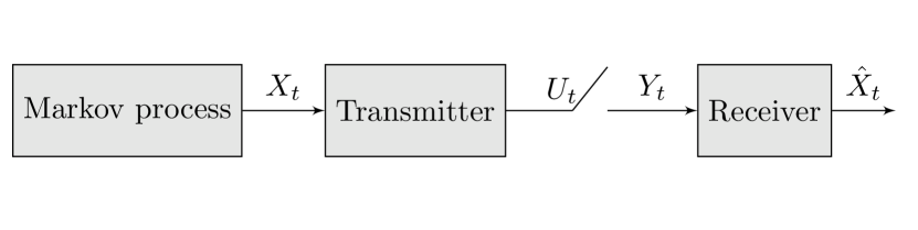
Figure 1: Block diagram of a remote estimation system.

Consider the following two models of a discrete-time Markov process $\{X_{t}\}_{t=0}^{\infty}$ with the initial state $X_{0}=0$ and for $t\geq 0$,

$$X_{t+1}=aX_{t}+W_{t},$$ (1)

where $\{W_{t}\}_{t=0}^{\infty}$ is an i.i.d. innovations process. We consider two specific models:

• Model A: $a,X_{t},W_{t}\in\mathds{Z}$ and $W_{t}$ is distributed according to a unimodal and symmetric pmf (probability mass function) $p$, i.e., for all $e\in\mathds{Z}_{\geq 0}$, $p_{e}=p_{-e}$ and $p_{e}\geq p_{e+1}$. To avoid trivial cases, we assume $p_{0}$ is strictly less than 1.

• Model B: $a,X_{t},W_{t}\in\mathds{R}$ and $W_{t}$ is distributed according to a unimodal, differentiable and symmetric pdf (probability density function) $\phi$, i.e., for all $e\in\mathds{R}_{\geq 0}$, $\phi(e)=\phi(-e)$ and for any $\delta\in\mathds{R}_{>0}$, $\phi(e)\geq\phi(e+\delta)$.

For uniformity of notation, define $\mathds{X}$ to be equal to $\mathds{Z}$ for Model A and equal to $\mathds{R}$ for Model B. $\mathds{X}_{\geq 0}$ and $\mathds{X}_{>0}$ are defined similarly.

A sensor sequentially observes the process and at each time, chooses whether or not to transmit the current state. This decision is denoted by $U_{t}\in\{0,1\}$, where $U_{t}=0$ denotes no transmission and $U_{1}=1$ denotes transmission. The decision to transmit is made using a transmission strategy $f=\{f_{t}\}_{t=0}^{\infty}$, where

$$U_{t}=f_{t}(X_{0:t},U_{0:t-1}).$$ (2)

We use the short-hand notation $X_{0:t}$ to denote the sequence $(X_{0},\dots,X_{t})$. Similar interpretations hold for $U_{0:t-1}$.

The transmitted symbol, which is denoted by $Y_{t}$, is given by

$$Y_{t}=\begin{cases}X_{t},&\text{if $U_{t}=1$};\\ \mathfrak{E},&\text{if $U_{t}=0$},\end{cases}$$

where $Y_{t}=\mathfrak{E}$ denotes no transmission.

The receiver sequentially observes $\{Y_{t}\}_{t=0}^{\infty}$ and generates an estimate $\{\hat{X}_{t}\}_{t=0}^{\infty}$, $\hat{X}\in\mathds{X}$, using an estimation strategy $g=\{g_{t}\}_{t=0}^{\infty}$, i.e.,

$$\hat{X}_{t}=g_{t}(Y_{0:t}).$$ (3)

The fidelity of the estimation is measured by a per-step distortion $d(X_{t}-\hat{X}_{t})$.

For both models, we assume the following:

• $d(0)=0$ and for $e\neq 0$, $d(e)>0$;

• $d(\cdot)$ is even, i.e., for all $e$, $d(e)=d(-e)$;

• $d(\cdot)$ is increasing, i.e., for $e_{1}>e_{2}>0$, $d(e_{1})\geq d(e_{2})$;

• For Model B, we assume that $d(\cdot)$ is differentiable.

We also characterize our results to the following special case of Model B:

• Gauss-Markov model: the density $\phi$ is zero-mean Gaussian with variance $\sigma^{2}$ and the distortion is quadratic, i.e.,

  $$\phi(e)=\frac{1}{\sqrt{2\pi}\sigma}\exp{\big{(}-e^{2}/(2\sigma^{2})\big{)}}\quad\text{and}\quad d(e)=e^{2}.$$

II-B Performance measures

Given a transmission and estimation strategy $(f,g)$ and a discount factor $\beta\in(0,1]$, we define the expected distortion and the expected number of transmissions as follows. For $\beta\in(0,1)$, the expected discounted distortion is given by

$$D_{\beta}(f,g)\coloneqq(1-\beta)\mathds{E}^{(f,g)}\Big{[}\sum_{t=0}^{\infty}\beta^{t}d(X_{t}-\hat{X}_{t})\Bigm{|}X_{0}=0\Big{]}$$ (4)

and for $\beta=1$, the expected long-term average distortion is given by

$$D_{1}(f,g)\coloneqq\limsup_{T\to\infty}\frac{1}{T}\mathds{E}^{(f,g)}\Big{[}\sum_{t=0}^{T-1}d(X_{t}-\hat{X}_{t})\Bigm{|}X_{0}=0\Big{]}.$$ (5)

Similarly, for $\beta\in(0,1)$, the expected discounted number of transmissions is given by

$$N_{\beta}(f,g)\coloneqq(1-\beta)\mathds{E}^{(f,g)}\Big{[}\sum_{t=0}^{\infty}\beta^{t}U_{t}\Bigm{|}X_{0}=0\Big{]}$$ (6)

and for $\beta=1$, the expected long-term average number of transmissions is given by

$$N_{1}(f,g)\coloneqq\limsup_{T\to\infty}\frac{1}{T}\mathds{E}^{(f,g)}\Big{[}\sum_{t=0}^{T-1}U_{t}\Bigm{|}X_{0}=0\Big{]}.$$ (7)

Remark 1.

We use a normalizing factor of $(1-\beta)$ to have a unified scaling for both discounted and long-term average setups. In particular, we will show that for any strategy $(f,g)$

$$C_{1}(f,g;\lambda)=\lim_{\beta\uparrow 1}C_{\beta}(f,g;\lambda),\quad\text{and}\quad D_{1}(f,g)=\lim_{\beta\uparrow 1}D_{\beta}(f,g).$$

Similar notation is used in [33].

II-C Problem formulations

We are interested in the following two optimization problems.

Problem 1 (Costly communication).

In the model of Section II-A, given a discount factor $\beta\in(0,1]$ and a communication cost $\lambda\in\mathds{R}_{>0}$, find a transmission and estimation strategy $(f^{*},g^{*})$ such that

$$C^{*}_{\beta}(\lambda)\coloneqq C_{\beta}(f^{*},g^{*};\lambda)=\inf_{(f,g)}C_{\beta}(f,g;\lambda),$$ (8)

where

$$C_{\beta}(f,g;\lambda)\coloneqq D_{\beta}(f,g)+\lambda N_{\beta}(f,g)$$

is the total communication cost and the infimum in (8) is taken over all history-dependent strategies.

Problem 2 (Constrained communication).

In the model of Section II-A, given a discount factor $\beta\in(0,1]$ and a constraint $\alpha\in(0,1)$, find a transmission and estimation strategy $(f^{*},g^{*})$ such that

$$D^{*}_{\beta}(\alpha)\coloneqq D_{\beta}(f^{*},g^{*})=\inf_{(f,g):N_{\beta}(f,g)\leq\alpha}D_{\beta}(f,g),$$ (9)

where the infimum is taken over all history-dependent strategies.

Remark 2.

It can be shown for $|a|\geq 1$ that $\lim_{\alpha\rightarrow 0}D^{*}_{1}(\alpha)=\infty$ and $\lim_{\alpha\rightarrow 1}D^{*}_{\beta}(\alpha)=0$.

The function $D_{\beta}^{*}(\alpha)$, $\beta\in(0,1]$, represents the minimum expected distortion that can be achieved when the expected number of transmissions are less than or equal to $\alpha$. It is analogous to the distortion-rate function in Information Theory; for that reason, we call it the distortion-transmission function.

III The main results

III-A Structure of optimal strategies

To completely characterize the functions $C^{*}_{\beta}(\lambda)$ and $D^{*}_{\beta}(\alpha)$, we first establish the structure of optimal transmitter and receiver.

Theorem 1 (Structural results).

Consider Problem 1 for $\beta\in(0,1]$. Then, for both Models A and B, we have the following.

1. Structure of optimal estimation strategy: The optimal estimation strategy $\hat{X}_{0}=0$ and for $t>0$ is as follows:

   $$\hat{X}_{t} =\begin{cases}Y_{t},&\mbox{if $Y_{t}\neq\mathfrak{E}$}\\ a\hat{X}_{t-1},&\mbox{if $Y_{t}=\mathfrak{E}$},\end{cases}$$

   or equivalently,

   $$\hat{X}_{t} =\begin{cases}X_{t},&\mbox{if $U_{t}=1$}\\ a\hat{X}_{t-1},&\mbox{if $U_{t}\neq 1$}.\end{cases}$$

   We denote this strategy by $g^{*}$.

2. Structure of optimal transmission strategy: Define $E_{t}\coloneqq X_{t}-a\hat{X}_{t-1}$, which we call the error process. Then there exists a time-invariant threshold $k$ such that the transmission strategy

   $$U_{t}=f^{(k)}(E_{t}) \coloneqq\begin{cases}1,&\mbox{if $|E_{t}|\geq k$}\\ 0,&\mbox{if $|E_{t}|<k$}\end{cases}$$ (10)

   is optimal.

The proof of the theorem is given in Section V.

Similar structural results were established for the finite horizon setup in [18, 1, 20], which we use to establish Theorem 1. See Section V for details. The transmission strategy of the form (10) are also called event-driven transmission or delta sampling.

Remark 3.

Each transmission resets the state of the error process to $w\in\mathds{X}$ with probability $p_{w}$ in Model A and with probability density $\phi(w)$ in Model B. In between the transmission, the error process evolves in a Markovian manner. Thus $\{E_{t}\}_{t=0}^{\infty}$ is a regenerative process.

III-B Performance of generic threshold-based strategies

Let $\mathcal{F}$ denote the class of all time-homogeneous threshold-based strategies of the form (10). For $\beta\in(0,1]$ and $e\in\mathds{X}$, define the following for a system that starts in state $e$ and follows strategy $f^{(k)}$:

• $L^{(k)}_{\beta}(e)$: the expected distortion until the first transmission;

• $M^{(k)}_{\beta}(e)$: the expected time until the first transmission;

• $D^{(k)}_{\beta}(e)$: the expected distortion;

• $N^{(k)}_{\beta}(e)$: the expected number of transmissions;

• $C^{(k)}_{\beta}(e;\lambda)$: the expected total cost, i.e.,

  $$C^{(k)}_{\beta}(e;\lambda)=D^{(k)}_{\beta}(e)+\lambda N^{(k)}_{\beta}(e),\quad\lambda\geq 0.$$

Note that $D^{(k)}_{\beta}(0)=D_{\beta}(f^{(k)},g^{*})$, $N^{(k)}_{\beta}(0)=N_{\beta}(f^{(k)},g^{*})$ and $C^{(k)}_{\beta}(0;\lambda)=C_{\beta}(f^{(k)},g^{*};\lambda)$.

Define $S^{(k)}$ as follows:

$$S^{(k)}\coloneqq\begin{cases}\{-(k-1),\cdots,k-1\},&\mbox{for Model A};\\ (-k,k),&\mbox{for Model B}.\end{cases}$$

Under strategy $f^{(k)}$, the transmitter does not transmit if $E_{t}\in S^{(k)}$. For that reason, we call $S^{(k)}$ the silent set. Define linear operator $\mathcal{B}^{(k)}$ as follows:

• Model A: For any $v^{(k)}:S^{(k)}\to\mathds{R}$, define operator $\mathcal{B}^{(k)}$ as

  $$[\mathcal{B}^{(k)}v](e)\coloneqq\sum_{n\in S^{(k)}}p_{n-ae}v(n),\quad\forall e\in S^{(k)}.$$

• Model B: For any $v^{(k)}:S^{(k)}\to\mathds{R}$, define operator $\mathcal{B}^{(k)}$ as

  $$[\mathcal{B}^{(k)}v](e)\coloneqq\int_{S^{(k)}}\phi(n-ae)v(n)dn,\quad\forall e\in S^{(k)}.$$

Recall from Remark 3 that the state $E_{t}$ evolves in a Markovian manner until the first transmission. We may equivalently consider the Markov process until it is absorbed in $(-\infty,-k]\cup[k,\infty)$. Thus, from balance equation for Markov processes, we have for all $e\in S^{(k)}$,

$$L^{(k)}_{\beta}(e) =d(e)+\beta[\mathcal{B}^{(k)}L^{(k)}_{\beta}](e),$$ (11)

$$M^{(k)}_{\beta}(e) =1+\beta[\mathcal{B}^{(k)}M^{(k)}_{\beta}](e).$$ (12)

Lemma 1.

For any $\beta\in(0,1]$, equations (11) and (12) have unique and bounded solutions $L^{(k)}_{\beta}$ and $M^{(k)}_{\beta}$ that are

1. strictly increasing in $k$,

2. continuous and differentiable in $k$ for Model B,

3. $\displaystyle\lim_{\beta\uparrow 1}L^{(k)}_{\beta}(e)=L^{(k)}_{1}(e)$, $\displaystyle\lim_{\beta\uparrow 1}M^{(k)}_{\beta}(e)=M^{(k)}_{1}(e)$, for all $e$.

The proof of the lemma is given in Appendix A.

Theorem 2 (Renewal relationships).

For any $\beta\in(0,1]$, the performance of strategy $f^{(k)}$ in both Models A and B is given as follows:

1. $D_{\beta}(f^{(0)},g^{*})=0$, $N_{\beta}(f^{(0)},g^{*})=1$, and $C_{\beta}(f^{(0)},g^{*};\lambda)=\lambda$.

2. For $k\in\mathds{X}_{>0}$,

   $$D_{\beta}(f^{(k)},g^{*}) =\frac{L^{(k)}_{\beta}(0)}{M^{(k)}_{\beta}(0)},$$

   $$N_{\beta}(f^{(k)},g^{*}) =\frac{1}{M^{(k)}_{\beta}(0)}-(1-\beta),$$

   and

   $$C_{\beta}(f^{(k)},g^{*};\lambda) =\frac{L^{(k)}_{\beta}(0)+\lambda}{M^{(k)}_{\beta}(0)}-\lambda(1-\beta).$$

The proof of the Theorem is given in Section VI.

Remark 4.

There is a $-1/(1-\beta)$ term in the expression of $N^{(k)}_{\beta}(0)$ because for $k>0$, $U_{0}=0$. Had we defined $U_{0}=1$, then we would have obtained the usual renewal relationship of $N^{(k)}_{\beta}(0)=1/M^{(k)}_{\beta}(0)$.

Thus, to compute $D_{\beta}(f^{(k)},g^{*})$ and $N_{\beta}(f^{(k)},g^{*})$, one needs to compute only $L^{(k)}_{\beta}(0)$ and $M^{(k)}_{\beta}(0)$. Computation of the latter expressions is given in the next section.

Proposition 1.

For both Models A and B,

1. $C^{(k)}_{\beta}(0;\lambda)$ is submodular in $(k,\lambda)$, i.e., for $l>k$, $C^{(l)}_{\beta}(0;\lambda)-C^{(k)}_{\beta}(0;\lambda)$ is decreasing in $\lambda$.

2. Let $k^{*}_{\beta}(\lambda)=\arg\inf_{k\geq 0}C^{(k)}_{\beta}(0;\lambda)$ be the optimal $k$ for a fixed $\lambda$. Then $k^{*}_{\beta}(\lambda)$ is increasing in $\lambda$.

The proof of the proposition is in Appendix B.

III-C Computation of $L^{(k)}_{\beta}$ and $M^{(k)}_{\beta}$

III-C1 Model A

For Model A, the values of $L^{(k)}_{\beta}$ and $M^{(k)}_{\beta}$ can be computed by observing that the operator $\mathcal{B}^{(k)}$ is equivalent to a matrix multiplication. In particular, define the matrix $P^{(k)}$ as

$$P^{(k)}_{ij}\coloneqq p_{i-j},\quad\forall i,j\in S^{(k)}.$$

Then,

$$[\mathcal{B}^{(k)}v](e)=\sum_{n\in S^{(k)}}p_{n-ae}v(n)=\sum_{n\in S^{(k)}}P^{(k)}_{n,ae}v(n)=[P^{(k)}v]_{ae}.$$ (13)

With a slight abuse of notation, we are using $v$ both as a function and a vector. Define the matrix $Q^{(k)}$ and the vector $d^{(k)}$ as follows:

$$Q^{(k)}_{\beta}\coloneqq[I_{2k-1}-\beta P^{(k)}]^{-1},\quad d^{(k)}\coloneqq[d(-k+1),\dots,d(k-1)]^{\intercal}.$$

Then, (11), (12) and (13) imply the following:

Proposition 2.

In Model A, for any $\beta\in(0,1]$,

$$L^{(k)}_{\beta} =[I_{2k-1}-\beta P^{(k)}]^{-1}d^{(k)}$$ (14)

$$M^{(k)}_{\beta} =[I_{2k-1}-\beta P^{(k)}]^{-1}\mathbf{1}_{2k-1}.$$ (15)

See Section III-F for an example of these calculations.

III-C2 Model B

For Model B, for any $\beta\in(0,1]$, (11) and (12) are Fredholm integral equations of second kind [34]. The solution can be computed by identifying the inverse operator

$$\mathcal{Q}^{(k)}_{\beta}=[I-\beta\mathcal{B}^{(k)}]^{-1},$$

which is given by

$$[\mathcal{Q}^{(k)}_{\beta}v](e)=\int_{-k}^{k}R^{(k)}_{\beta}(e,w;a)v(w)dw,$$ (16)

where for any given $a$, $R^{(k)}_{\beta}(\cdot,\cdot;a)$ is the resolvent of $\phi$ and can be computed using the Liouville-Neumann series. See [34] for details. Since $\phi$ is smooth, (11) and (12) can also be solved by discretizing the integral equation using quadrature methods. A Matlab implementation of this approach is available in [35].

III-D Main results for Model A

III-D1 Results for costly communication

(a)

(b)

Figure 2: In Model A, (a) the optimal costly communication cost $C^{*}_{\beta}(\lambda)$; (b) the distortion-transmission function $D^{*}_{\beta}(\alpha)$.

Theorem 3.

For $\beta\in(0,1]$, let $\mathds{K}$ denote $\{k\in\mathds{Z}_{\geq 0}:D^{(k+1)}_{\beta}(0)>D^{(k)}_{\beta}(0)\}$. For $k_{n}\in\mathds{K}$, define:

$$\lambda^{(k_{n})}_{\beta}\coloneqq\frac{D^{(k_{n+1})}_{\beta}(0)-D^{(k_{n})}_{\beta}(0)}{N^{(k_{n})}_{\beta}(0)-N^{(k_{n+1})}_{\beta}(0)}.$$ (17)

Then, we have the following.

1. For any $k_{n}\in\mathds{K}$ and any $\lambda\in(\lambda^{(k_{n-1})}_{\beta},\lambda^{(k_{n})}_{\beta}]$, the strategy $f^{(k_{n})}$ is optimal for Problem 1 with communication cost $\lambda$.

2. The optimal performance $C^{*}_{\beta}(\lambda)$ is continuous, concave, increasing and piecewise linear in $\lambda$. The corner points of $C^{*}_{\beta}(\lambda)$ are given by $\{(\lambda^{(k_{n})}_{\beta},D^{(k_{n})}_{\beta}(0)+\lambda^{(k_{n})}_{\beta}N^{(k_{n})}_{\beta}(0))\}_{k_{n}\in\mathds{K}}$ (see Fig 2(a)(a)).

The proof of the theorem is given in Section VII.

III-D2 Results for constrained communication

To describe the solution of Problem 2, we first define Bernoulli randomized strategy and Bernoulli randomized simple strategy [36].

Definition 1.

Suppose we are given two (non-randomized) time-homogeneous strategies $f_{1}$ and $f_{2}$ and a randomization parameter $\theta\in(0,1)$. The Bernoulli randomized strategy $(f_{1},f_{2},\theta)$ is a strategy that randomizes between $f_{1}$ and $f_{2}$ at each stage; choosing $f_{1}$ with probability $\theta$ and $f_{2}$ with probability $(1-\theta)$. Such a strategy is called a Bernoulli randomized simple strategy if $f_{1}$ and $f_{2}$ differ on exactly one state, i.e., there exists a state $e_{0}$ such that

$$f_{1}(e)=f_{2}(e),\quad\forall e\neq e_{0}.$$

Theorem 4.

For any $\beta\in(0,1]$ and $\alpha\in(0,1)$, define

$$k^{*}_{\beta}(\alpha) =\sup\{k\in\mathds{Z}_{\geq 0}:N_{\beta}(f^{(k)},g^{*})\geq\alpha\}$$

$$=\sup\Big{\{}k\in\mathds{Z}_{\geq 0}:M^{(k)}_{\beta}\leq\frac{1}{1+\alpha-\beta}\Big{\}}$$ (18)

and

$$\theta^{*}_{\beta}(\alpha) =\frac{\alpha-N_{\beta}(f^{(k^{*}_{\beta}(\alpha)+1)},g^{*})}{N_{\beta}(f^{(k^{*}_{\beta}(\alpha))},g^{*})-N_{\beta}(f^{(k^{*}_{\beta}(\alpha)+1)},g^{*})}$$

$$=\frac{M^{(k^{*}+1)}_{\beta}-\frac{1}{1+\alpha-\beta}}{M^{(k^{*}+1)}_{\beta}-M^{(k^{*})}_{\beta}}.$$ (19)

For ease of notation, we use $k^{*}=k^{*}_{\beta}(\alpha)$ and $\theta^{*}=\theta^{*}_{\beta}(\alpha)$.

Let $f^{*}$ be the Bernoulli randomized simple strategy $(f^{(k^{*})},f^{(k^{*}+1)},\theta^{*})$, i.e.,

$$f^{*}(e)=\begin{cases}0,&\text{if $|e|<k^{*}$};\\ 0,&\text{w.p. $1-\theta^{*}$, if $|e|=k^{*}$};\\ 1,&\text{w.p. $\theta^{*}$, if $|e|=k^{*}$};\\ 1,&\text{if $|e|>k^{*}$}.\end{cases}$$ (20)

Then

1. $(f^{*},g^{*})$ is optimal for the constrained Problem 2 with constraint $\alpha$.

2. Let $\alpha^{(k)}=N_{\beta}(f^{(k)},g^{*})$. Then, for $\alpha\in(\alpha^{(k+1)},\alpha^{(k)})$, $k^{*}=k$ and $\theta^{*}=(\alpha-\alpha^{(k+1)})/(\alpha^{(k)}-\alpha^{(k+1)})$, and the distortion-transmission function is given by

   $$D^{*}_{\beta}(\alpha)=\theta^{*}D_{\beta}^{(k)}+(1-\theta^{*})D_{\beta}^{(k+1)}.$$ (21)

   Moreover, the distortion-transmission function is is continuous, convex, decreasing and piecewise linear in $\alpha$. Thus, the corner points of $D^{*}_{\beta}(\alpha)$ are given by $\{(N^{(k)}_{\beta}(0),D^{(k)}_{\beta}(0))\}_{k=1}^{\infty}$ (see Fig 2(a)(b)).

The proof of the theorem is given in Section VII.

Corollary 1.

In Model A, for any $\beta\in(0,1]$,

$$D_{\beta}(f^{(1)},g^{*})=0,\quad\text{and}\quad N_{\beta}(f^{(1)},g^{*})=\beta(1-p_{0})\coloneqq\alpha_{c}.$$

III-E Main results for Model B

III-E1 Results for costly communication

Let $\partial_{k}D^{(k)}_{\beta}$, $\partial_{k}N^{(k)}_{\beta}$ and $\partial_{k}C^{(k)}_{\beta}$ denote the derivative of $D^{(k)}_{\beta}$, $N^{(k)}_{\beta}$ and $C^{(k)}_{\beta}$ with respect to $k$ (in Lemma 6 we show that $D^{(k)}_{\beta}$, $N^{(k)}_{\beta}$ and $C^{(k)}_{\beta}$ are differentiable in $k$).

Theorem 5.

For $\beta\in(0,1]$, we have the following.

1. If the pair $(\lambda,k)$ satisfies the following

   $$\lambda=-\frac{\partial_{k}D^{(k)}_{\beta}(0)}{\partial_{k}N^{(k)}_{\beta}(0)},$$ (22)

   then, the strategy $(f^{(k)},g^{*})$ is optimal for Problem 1 with communication cost $\lambda$. Furthermore, for any $k>0$, there exists a $\lambda\geq 0$ that satisfies (22).

2. The optimal performance $C^{*}_{\beta}(\lambda)$ is continuous, concave and increasing function of $\lambda$.

The proof of the theorem is given in Section VIII. Algorithm 1 shows how to compute $C^{*}_{\beta}(\lambda)$.

input : $\lambda\in\mathds{R}_{>0}$, $\beta\in(0,1]$, $\varepsilon\in\mathds{R}_{>0}$

output : $C^{(k^{\circ})}_{\beta}(\lambda)$, where $|k^{\circ}-k^{*}_{\beta}(\lambda)|<\varepsilon$

Let $\lambda^{*}_{\beta}(k)$ denote the left-hand side of (22)

Pick $\underline{k}$ and $\bar{k}$ such that $\lambda^{*}_{\beta}(\underline{k})<\lambda<\lambda^{*}_{\beta}(\bar{k})$

$k^{\circ}=(\underline{k}+\bar{k})/2$

while $|\lambda^{*}_{\beta}(k^{\circ})-\lambda|>\varepsilon$ do

       if $\lambda^{*}(k^{\circ})<\lambda$ then

            $\underline{k}=k^{\circ}$

       else

            $\bar{k}=k^{\circ}$

      $k^{\circ}=(\underline{k}+\bar{k})/2$

      

return $D^{(k^{\circ})}_{\beta}(0)+\lambda N^{(k^{\circ})}_{\beta}(0)$

Algorithm 1 Computation of $C^{*}_{\beta}(\lambda)$

III-E2 Results for constrained communication

Theorem 6.

For any $\beta\in(0,1]$ and $\alpha\in(0,1)$, let $k^{*}_{\beta}(\alpha)\in\mathds{R}_{\geq 0}$ be such that

$$N_{\beta}^{(k^{*}_{\beta}(\alpha))}(0)=\alpha.$$ (23)

Such a $k^{*}_{\beta}(\alpha)$ always exists and we have the following:

1. The strategy $(f^{(k^{*}_{\beta}(\alpha))},g^{*})$ is optimal for Problem 2 with constraint $\alpha$.

2. The distortion-transmission function $D^{*}_{\beta}(\alpha)$ is continuous, convex and decreasing in $\alpha$ and is given by

   $$D^{*}_{\beta}(\alpha)=D_{\beta}^{(k^{*}_{\beta}(\alpha))}(0).$$ (24)

The proof of the theorem is given in Section VIII. Algorithm 2 shows how to compute $D^{*}_{\beta}(\alpha)$.

input : $\alpha\in(0,1)$, $\beta\in(0,1]$, $\varepsilon\in\mathds{R}_{>0}$

output : $D^{(k^{\circ})}_{\beta}(\alpha)$, where $|N^{(k^{\circ})}_{\beta}(0)-\alpha|<\varepsilon$

Pick $\underline{k}$ and $\bar{k}$ such that $N^{(\underline{k})}_{\beta}(0)<\alpha<N^{(\bar{k})}_{\beta}(0)$

$k^{\circ}=(\underline{k}+\bar{k})/2$

while $|N^{(k^{\circ})}_{\beta}(0)-\alpha|>\varepsilon$ do

       if $N^{(k^{\circ})}_{\beta}(0)<\alpha$ then

            $\underline{k}=k^{\circ}$

       else

             $\bar{k}=k^{\circ}$

      $k^{\circ}=(\underline{k}+\bar{k})/2$

      

return $D^{(k^{\circ})}_{\beta}(\alpha)$

Algorithm 2 Computation of $D^{*}_{\beta}(\alpha)$

III-E3 Special case of Model B–Gauss-Markov model

In general, the optimal thresholds, and the functions $C^{*}_{\beta}(\lambda)$ and $D^{*}_{\beta}(\alpha)$ depend on the noise distribution $\phi(\cdot)$. For the Gauss-Markov model, the dependence on the variance $\sigma^{2}$ of the noise may be quantified exactly.

For ease of notation, we drop the dependence on $\beta$ from the notation, and instead, show the dependence on $\sigma$. Thus, $C^{*}_{\sigma}(\lambda)$ denotes the optimal value for the costly communication case when the noise variance is $\sigma^{2}$. Similar notation holds for other terms.

Theorem 7.

For the Gauss-Markov model for Problem 1, $k^{*}_{\sigma}(\lambda)=k^{*}_{1}(\lambda/a^{2}\sigma^{2})$ and $C^{*}_{\sigma}(\lambda)=\sigma^{2}C^{*}_{1}(\lambda/\sigma^{2})$. For Problem 2, $k^{*}_{\sigma}(\alpha)=\sigma k^{*}_{1}(\alpha)$ and $D^{*}_{\sigma}(\alpha)=\sigma^{2}D^{*}_{1}(\alpha)$.

The proof of the theorem is given in Section VIII.

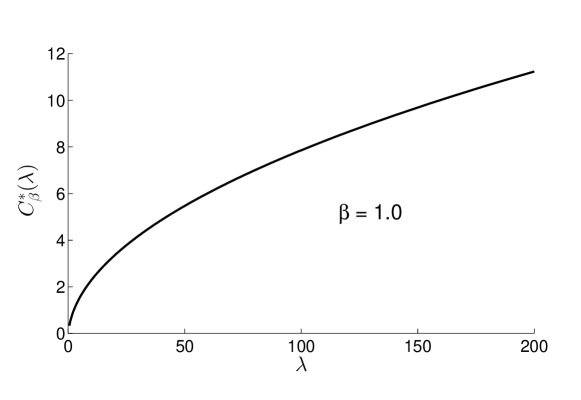
(a)

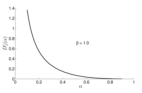
(b)

Figure 3: Gauss-Markov model ($\sigma^{2}=1$ and $a=1$): (a) optimal costly communication cost $C^{*}_{1}(\alpha)$; (b) distortion-transmission function $D^{*}_{1}(\alpha)$.

An implication of the above theorem is that we only need to numerically compute $C^{*}_{1}(\lambda)$ and $D^{*}_{1}(\alpha)$, which are shown in Fig. 3. The optimal total communication cost and the distortion-transmission function for any other value $\sigma^{2}$ can be obtained by simply scaling $C^{*}_{1}(\lambda)$ and $D^{*}_{1}(\alpha)$ respectively.

III-F An example for Model A: symmetric birth-death Markov chain

An example of a Markov process and a distortion function that satisfy Model A is the following:

TABLE I: Values of $D^{(k)}_{\beta}$, $N^{(k)}_{\beta}$ and $\lambda^{(k)}_{\beta}$ for different values of $k$ and $\beta$ for the Markov chain of Example 1 with $p=0.3$. Note that $D^{(0)}_{\beta}(0)=D^{(1)}_{\beta}(0)$; therefore $\mathds{K}$ defined in Theorem 3 equals $\mathds{Z}_{>0}$.

(a) For $\beta=0.9$

$k$	$D^{(k)}_{\beta}(0)$	$N^{(k)}_{\beta}(0)$	$\lambda^{(k)}_{\beta}$
0	0	1	–
1	0	0.5400	1.0989
2	0.4576	0.1236	4.1021
3	0.7695	0.0475	9.2839
4	1.0066	0.0220	16.2509
5	1.1844	0.0111	24.4478
6	1.3130	0.0058	33.4121
7	1.4029	0.0031	42.8289
8	1.4638	0.0017	52.5042
9	1.5040	0.0009	62.3245
10	1.5298	0.0005	72.2255

(b) For $\beta=0.95$

$k$	$D^{(k)}_{\beta}(0)$	$N^{(k)}_{\beta}(0)$	$\lambda^{(k)}_{\beta}$
0	0	1	–
1	0	0.5700	1.1050
2	0.4790	0.1365	4.3657
3	0.8282	0.0565	10.6058
4	1.1218	0.0288	19.9550
5	1.3715	0.0163	32.0869
6	1.5811	0.0098	46.4727
7	1.7536	0.0061	62.5651
8	1.8927	0.0039	79.8921
9	2.0028	0.0025	98.0854
10	2.0884	0.0016	116.8739

(c) For $\beta=1.0$

$k$	$D^{(k)}_{\beta}(0)$	$N^{(k)}_{\beta}(0)$	$\lambda^{(k)}_{\beta}$
0	0	1	–
1	0	0.6000	1.1111
2	0.5000	0.1500	4.6667
3	0.8889	0.0667	12.3810
4	1.2500	0.0375	25.9259
5	1.6000	0.0240	46.9697
6	1.9444	0.0167	77.1795
7	2.2857	0.0122	118.2222
8	2.6250	0.0094	171.7647
9	2.9630	0.0074	239.4737
10	3.0000	0.0060	323.0159

Example 1.

Consider a Markov chain of the form (1) where the pmf of $W_{t}$ is given by

$$p_{n}=\begin{cases}p,&\text{if $|n|=1$}\\ 1-2p,&\text{if $n=0$}\\ 0,&\text{otherwise},\end{cases}$$

where $p\in(0,\frac{1}{3})$. The distortion function is taken as $d(e)=|e|$.

This Markov process corresponds to a symmetric, birth-death Markov chain defined over $\mathds{Z}$ as shown in Fig. 4, with the transition probability matrix is given by

$$P_{ij}=\begin{cases}p,&\text{if $|i-j|=1$};\\ 1-2p,&\text{if $i=j$};\\ 0,&\text{otherwise}.\end{cases}$$

Figure 4: A birth-death Markov chain

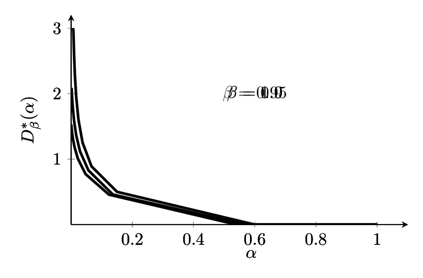
(a) $D^{*}_{\beta}(\alpha)$ vs $\alpha$ for $\beta=0.9$

(b) $D^{*}_{\beta}(\alpha)$ vs $\alpha$ for $\beta=0.95$

(c) $D^{*}_{\beta}(\alpha)$ vs $\alpha$ for $\beta=1.0$

Figure 5: Plots of $D^{*}_{\beta}(\alpha)$ vs $\alpha$ for different $\beta$ for the birth-death Markov chain of Example 1 with $p=0.3$.

III-F1 Performance of a generic threshold-based strategy

Lemma 2.

1. For $\beta\in(0,1)$,

   $$D^{(k)}_{\beta}(0) =\frac{\sinh(km_{\beta})-k\sinh(m_{\beta})}{2\sinh^{2}(km_{\beta}/2)\sinh(m_{\beta})};$$

   $$N^{(k)}_{\beta}(0) =\frac{2\beta p\sinh^{2}(m_{\beta}/2)\cosh(km_{\beta})}{\sinh^{2}(km_{\beta}/2)}-(1-\beta).$$

2. For $\beta=1$,

   $$D^{(k)}_{1}=\frac{k^{2}-1}{3k};\quad N^{(k)}_{1}=\frac{2p}{k^{2}};$$

and

$$\lambda^{(k)}_{1}=\frac{k(k+1)(k^{2}+k+1)}{6p(2k+1)}.$$

The proof is given in Section IX.

III-F2 Optimal strategy for costly communication

Using the above expressions for $D^{(k)}_{\beta}(0)$ and $N^{(k)}_{\beta}(0)$, we can identify $\mathds{K}$ and for each $k_{n}\in\mathds{K}$, compute $\lambda^{(k_{n})}_{\beta}$ according to (17). These values are tabulated in Table I for different values of $\beta$ (all for $p=0.3$). Using Table I, we can compute the corner points $(\lambda^{(k_{n})}_{\beta},D^{(k_{n})}_{\beta}(0)+\lambda^{(k_{n})}_{\beta}N^{(k_{n})}_{\beta}(0))$ of $C^{*}_{\beta}(\lambda)$. Joining these points by straight lines gives $C^{*}_{\beta}(\lambda)$, as shown in Fig. 6. The optimal strategy for a given $\lambda$ can be computed from Table I.

Figure 6: Plot of $C^{*}_{\beta}(\lambda)$ vs $\lambda$ for the Markov chain of Example 1 with $p=0.3$.

For example, for $\lambda=20$, $\beta=0.9$, we can find from Table I(a) that $\lambda\in(\lambda^{(4)}_{\beta},\lambda^{(5)}_{\beta}]$. Hence, $k^{*}_{\beta}=5$ (i.e., the strategy $f^{(5)}$ is optimal) and the optimal total communication cost is

$$C^{*}_{0.9}(20)=D^{(5)}_{0.9}(0)+20N^{(5)}_{0.9}(0)=1.1844+20\times 0.0111=1.4064.$$

III-F3 Optimal strategy for constrained communication

Using the values in Table I, we can also compute the corner points $(N^{(k)}_{\beta}(0),D^{(k)}_{\beta}(0))$ of $D^{*}_{\beta}(\alpha)$. Joining these points by straight lines gives $D^{*}_{\beta}(\alpha)$ (see Fig. 5). The optimal strategy for a given $\alpha$ can be computed from Table I. For example, at $\alpha=0.1$ and $\beta=0.9$, $k^{*}_{\beta}(\alpha)$ is the largest value of $k$ such that $N^{(k)}_{\beta}(0)\geq\alpha$. Thus, from Table I(a), we get that $k^{*}=2$. Then, by (23),

$$\theta^{*}=\frac{\alpha-N^{(3)}_{\beta}}{N^{(2)}_{\beta}-N^{(3)}_{\beta}}=0.6899.$$

Let $f^{*}=(f^{(2)},f^{(3)},\theta^{*})$. Then the Bernoulli randomized simple strategy $(f^{*},g^{*})$ is optimal for Problem 2 for $\beta\in(0,1)$. Furthermore, by (21), $D^{*}_{\beta}(\alpha)=0.5543$.

IV Salient features and discussion

IV-A Comparison with periodic and randomized strategies

In our model, we assume that the transmission decision depends on the state of the Markov process. In some of the remote estimation literature, it is assumed that the transmission schedule does not depend on the state of the Markov process. Two such commonly used strategies are:

1. Periodic transmission strategy with period $T$:

   $$U_{t}=f_{p}(t\text{ mod }T),$$

   where $\sum_{t=0}^{T-1}f_{p}(t)=1/\alpha$.

2. Random transmission strategy:

   $$U_{t}=\begin{cases}1,&\mbox{w.p. $\alpha$}\\ 0,&\mbox{w.p. $1-\alpha$}.\end{cases}$$

Below, we compare the performance of the threshold-based strategy with these two strategies for the for the long-term average setup for Problem 2 for Model B with $a=1$.

IV-A1 Performance of the periodic strategy

In general, the performance of a periodic transmission strategy depends on the choice of transmission function $f_{p}$. For ease of calculation we consider the values of $(\alpha,T)$ for which $f_{p}$ is unique.

1. $\alpha=1/T$, $T\in\mathds{Z}_{>0}$, i.e., the transmitter remains silent for $(T-1)$ steps and then transmits once. The expected distortion in this case is

   $$D_{\text{per}}(\alpha) =\frac{1}{T}\mathds{E}\Big{[}\sum_{t=0}^{T-1}E^{2}_{t}\Big{]}$$

   $$\stackrel{{\scriptstyle(a)}}{{=}}\frac{1}{T}\mathds{E}\Big{[}\sum_{t=0}^{T-1}t\sigma^{2}\Big{]}=\frac{1}{T}\frac{(T-1)T}{2}\sigma^{2}=\frac{\sigma^{2}}{2}\big{(}\frac{1}{\alpha}-1\big{)},$$

   where $(a)$ uses $E_{t}=W_{0}+W_{1}+W_{2}+\cdots+W_{t-1}$.

2. $\alpha=(T-1)/T$, $T\in\mathds{Z}_{>0}$, i.e., the transmitter remains silent for 1 step and then transmits for $(T-1)$ steps. The expected distortion in this case is

   $$D_{\text{per}}(\alpha)=\frac{1}{T}\mathds{E}[E^{2}_{1}]=\frac{\sigma^{2}}{T}=\sigma^{2}(1-\alpha).$$

IV-A2 Performance generic stationary transmission strategy

Next, we derive an expression of $D_{\beta}(f,g^{*})$ for arbitrary stationary transmission strategy $f$ (that does not use the value of the state $E_{t}$ to determine when to transmit; so the receiver is the same as in Theorem 1) for the long-term average setup for Model B when $a=1$.

Proposition 3.

For $\beta=1$ and $a=1$ in Model B, let $f$ be an arbitrary stationary transmission strategy. Let $\tau$ denote the stopping time of the first transmission under $f$. Then

$$D_{1}(f,g^{*})=\frac{\sigma^{2}}{2}\Big{[}\frac{\mathds{E}(\tau^{2})}{\mathds{E}(\tau)}-1\Big{]}.$$

Proof:

For any $t<\tau$, $E_{t}=W_{0}^{2}+\dots+W_{t-1}^{2}$. Therefore, $\mathds{E}[E^{2}_{t}]=t\sigma^{2}$ and define $\hat{L}(t)=\sum_{s=1}^{t-1}\mathds{E}[E_{s}^{2}]=\frac{1}{2}t(t-1)\sigma^{2}$. Now, $L_{1}(0)=\mathds{E}[\hat{L}(\tau)]=(\sigma^{2}/2)[\mathds{E}(\tau^{2})-\mathds{E}(\tau)]$ and $M_{1}(0)=\mathds{E}(\tau)$. By using the same argument as in the proof of Theorem 2, we get $D_{1}(f,g^{*})=L_{1}(0)/M_{1}(0)$, which implies the result.

IV-A3 Performance of randomized transmission strategy

For the randomized strategy defined above, $\tau$ is a $\text{Geom}_{1}(\alpha)$ random variable. Therefore, $\mathds{E}(\tau^{2})=2/\alpha^{2}-1/\alpha$ and $\mathds{E}(\tau)=1/\alpha$. Hence, following Proposition 3, we have

$$D_{\text{rand}}(\alpha)=\sigma^{2}\big{[}\frac{1}{\alpha}-1\big{]}.$$

Fig. 7 shows that threshold-based startegy performs considerably well compared to the periodic transmission strategy and the randomized transmission strategy.

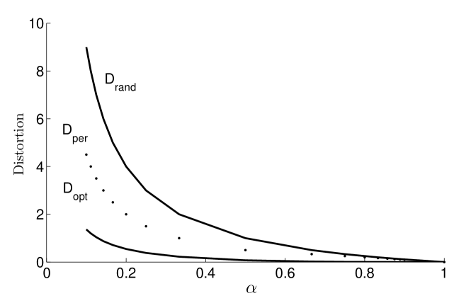
Figure 7: Comparison of the performances of the threshold-based startegy (denoted by $D_{\text{opt}}$) with periodic and randomized transmission strategies (denoted by $D_{\text{per}}$ and $D_{\text{rand}}$, respectively) for a Gauss-Markov process with $a=1$ and $\sigma^{2}=1$.

IV-B Discussion on deterministic implementation

The optimal strategy shown in Theorem 4 chooses a randomized action in states $\{-k^{*},k^{*}\}$. It is also possible to identify deterministic (non-randomized) but time-varying strategies that achieve the same performance. We describe two such strategies for the long-term average setup.

IV-B1 Steering strategies

Let $a^{0}_{t}$ (respectively, $a^{1}_{t}$) denote the number of times the action $u_{t}=0$ (respectively, the action $u_{t}=1$) has been chosen in states $\{-k^{*},k^{*}\}$ in the past, i.e.

$$a^{i}_{t}=\sum_{s=0}^{t-1}\mathds{1}\{|E_{s}|=k^{*},\,u_{s}=i\},\quad i\in\{0,1\}.$$

Thus, the empirical frequency of choosing action $u_{t}=i$, $i\in\{0,1\}$, in states $\{-k^{*},k^{*}\}$ is $a^{i}_{t}/(a^{0}_{t}+a^{1}_{t})$. A steering strategy compares these empirical frequencies with the desired randomization probabilities $\theta^{0}=1-\theta^{*}$ and $\theta^{1}=\theta^{*}$ and chooses an action that steers the empirical frequency closer to the desired randomization probability. More formally, at states $\{-k^{*},k^{*}\}$, the steering transmission strategy chooses the action

$$\arg\min_{i}\Big{\{}\theta^{i}-\frac{a^{i}_{t}+1}{a^{0}_{t}+a^{1}_{t}+1}\Big{\}}$$

in states $\{-k^{*},k^{*}\}$ and chooses deterministic actions according to $f^{*}$ (given in (20)) in states except $\{-k^{*},k^{*}\}$. Note that the above strategy is deterministic (non-randomized) but depends on the history of visits to states $\{-k^{*},k^{*}\}$. Such strategies were proposed in [37], where it was shown that the steering strategy descibed above achieves the same performance as the randomized startegy $f^{*}$ and hence is optimal for Problem 2 for $\beta=1$. Variations of such steering strategies have been proposed in [38, 39], where the adaptation was done by comparing the sample path average cost with the expected value (rather than by comparing empirical frequencies).

IV-B2 Time-sharing strategies

Define a cycle to be the period of time between consecutive visits of process $\{E_{t}\}_{t=0}^{\infty}$ to state zero. A time-sharing strategy is defined by a series $\{(a_{m},b_{m})\}_{m=0}^{\infty}$ and uses startegy $f^{(k^{*})}$ for the first $a_{0}$ cycles, uses startegy $f^{(k^{*}+1)}$ for the next $b_{0}$ cycles, and continues to alternate between using startegy $f^{(k^{*})}$ for $a_{m}$ cycles and strategy $f^{(k^{*}+1)}$ for $b_{m}$ cycles. In particular, if $(a_{m},b_{m})=(a,b)$ for all $m$, then the time-sharing strategy is a periodic strategy that uses $f^{(k^{*})}$ $a$ cycles and $f^{(k^{*}+1)}$ for $b$ cycles.

The performance of such time-sharing strategies was evaluated in [40], where it was shown that if the cycle-lengths of the time-sharing strategy are chosen such that,

$$\lim_{M\to\infty}\frac{\sum_{m=0}^{M}a_{m}}{\sum_{m=0}^{M}(a_{m}+b_{m})} =\frac{\theta^{*}N^{(k^{*})}_{1}}{\theta^{*}N^{(k^{*})}_{1}+(1-\theta^{*})N^{(k^{*}+1)}_{1}}$$

$$=\frac{\theta^{*}N^{(k^{*})}_{1}}{\alpha},$$

then the time-sharing strategy $\{(a_{m},b_{m})\}_{m=0}^{\infty}$ achieves the same performance as the randomized strategy $f^{*}$ and hence, is optimal for Problem 2 for $\beta=1$.

V Proof of the structural result: Theorem 1

V-A Finite horizon setup

A finite horizon version of Problem 1 has been investigated in [1] (for Model A) and in [18, 20] (for Model B), where the structure of the optimal transmission and estimation strategy was established.

Theorem 8.

[18, 1, 20] For both Models A and B, for a finite horizon version of Problem 1, we have the following.

1. Structure of optimal estimation strategy: the estimation strategy defined in Theorem 1 is optimal.

2. Structure of optimal transmission strategy: define $E_{t}$ as in Theorem 1. Then there exist threholds $\{k_{t}\}_{t=1}^{T}$ such that the transmission strategy

   $$U_{t}\coloneqq f_{t}(E_{t})=\begin{cases}1,&\text{if $|E_{t}|\geq k_{t}$};\\ 0,&\text{if $|E_{t}|<k_{t}$}\end{cases}$$ (25)

   is optimal.

The above structural results were obtained in [1, Theorems 2 and 3] for Model A and in [18, Theorem 1] and [20, Lemmas 1, 3 and 4] of Model B.

Remark 5.

The results in [1] were derived under the assumption that $\{W_{t}\}$ has finite support. These results can be generalized for $\{W_{t}\}$ having countable support using ideas from [3]. For that reason, we state Theorem 8 without any restriction on the support of $\{W_{t}\}$. See the supplementary document for the generalization of [1, Theorems 2 and 3] to $\{W_{t}\}$ with countable support.

V-B Infinite horizon setup

In a general real-time communication system, the optimal estimation strategy depends on the choice of the transmission strategy and vice-versa. Theorem 8 shows that when the noise process and the distortion function satisfy appropriate symmetry assumptions, the optimal estimation strategy can be specified in closed form. Consequently, we can fix the estimation strategy to be of the above form and consider the optimization problem of identifying the best transmission strategy. This optimization problem has a single decision maker—the transmitter—and we use techniques from centralized stochastic control to solve it. Since the optimal estimation strategy is time-homogeneous, one expects the optimal transmission strategy (i.e., the choice of the optimal thresholds $\{k_{t}\}_{t=0}^{\infty}$) to be time-homogeneous as well. The technical difficulty in establishing such a result is that the state space is not compact and the distortion function may be unbounded.

To prove Theorem 1, we proceed as follows:

1. We show that the result of the theorem is true for $\beta\in(0,1)$ and the optimal strategy is given by an appropriate dynamic program.

2. We show that for the discounted setup, the value function of the dynamic program is even and increasing on $\mathds{X}$.

3. For $\beta=1$, we use the vanishing discount approach to show that the optimal strategy for the long-term average cost setup may be determined as a limit to the optimal strategy for the discounted cost setup is the discount factor $\beta\uparrow 1$.

V-B1 The discounted setup

Lemma 3.

In Model A. an optimal transmission strategy is given by the unique and bounded solution of the following dynamic program: for all $e\in\mathds{Z}$,

$$V_{\beta}(e;\lambda) =\min\Big{[}(1-\beta)\lambda+\beta\sum_{w\in\mathds{Z}}p_{w}V_{\beta}(w;\lambda),$$

$$\quad(1-\beta)d(e)+\beta\sum_{w\in\mathds{Z}}p_{w}V_{\beta}(ae+w;\lambda)\Big{]}.$$ (26)

Proof:

When $d(\cdot)$ is bounded, the per-step cost $c(e,u)\coloneqq(1-\beta)[\lambda u+d(e)(1-u)]$, $u\in\{0,1\}$, for a given $\lambda$ is also bounded and hence according to [42, Proposition 4.7.1, Theorem 4.6.3], there exists the unique and bounded solution $V_{\beta}(e;\lambda)$ of the dynamic program (26).

When $d(\cdot)$ is unbounded, then for any communication cost $\lambda$, we first define $e_{0}\in\mathds{Z}_{\geq 0}<\infty$ as:

$$e_{0}\coloneqq\min\Big{\{}e\,:\,d(e)\geq\frac{\lambda}{1-\beta}\Big{\}}.$$

Now, for any state $e$, $|e|>e_{0}$, the per-step cost $(1-\beta)d(e)$ of not transmitting is greater then the cost of transmitting at each step in the future, which is given by $(1-\beta)\sum_{t=0}^{\infty}\beta^{t}\lambda=\lambda$. Thus, the optimal action is to transmit, i.e., $f^{*}(e)=1$. Hence, the dynamic program can be written as

$$V_{\beta}(e;\lambda)=\min\{V^{0}_{\beta}(e;\lambda),V^{1}_{\beta}(e;\lambda)\},$$

where

$$V^{0}_{\beta}(e;\lambda) =(1-\beta)d(e)+\beta\sum_{w\in\mathds{Z}}p_{w}V_{\beta}(ae+w;\lambda),$$

$$V^{1}_{\beta}(e;\lambda) =(1-\beta)\lambda+\beta\sum_{w\in\mathds{Z}}p_{w}V_{\beta}(w;\lambda).$$

Let $\mathcal{E}^{*}\coloneqq\{e\,:\,|e|\geq e_{0}\}$. Then, for all $e\in\mathcal{E}^{*}$, $V_{\beta}(e;\lambda)$ is constant. Thus, (26) is equivalent to a finite-state Markov decision process with state space $\{-e_{0}+1,\cdots,e_{0}-1\}\cup e^{*}$ (where $e^{*}$ is a generic state for all states in the set $\mathcal{E}^{*}$). Since the state space is now finite, the dynamic program (26) has a unique and bounded time-homogeneous solution by the argument given for bounded $d(\cdot)$.

Lemma 4.

In Model B, an optimal transmission strategy is given by the unique and bounded solution of the following dynamic program: for all $e\in\mathds{R}$,

$$V_{\beta}(e;\lambda)=\min\Big{[}(1-\beta)\lambda+\beta\int_{\mathds{R}}\phi(w)V_{\beta}(w;\lambda)dw,\\ \qquad(1-\beta)d(e)+\beta\int_{\mathds{R}}\phi(w)V_{\beta}(ae+w;\lambda)dw\Big{]}.$$ (27)

Proof:

When $d(\cdot)$ is bounded, the per-step cost $c(e,u)$, as defined in part (a), for a given $\lambda$ is also bounded. Let $K=(1-\beta)\sup_{e\in\mathds{R}}\{d(e)\}$. Then, the strategy ‘always transmit’ satisfies [43, Assumption 4.2.2] with $V_{\beta}(e;\lambda)\leq K/(1-\beta)$. Also, $\lambda$, $d(\cdot)$ and $\phi(\cdot)$ satisfy [43, Assumption 4.2.1]. Hence, the above dynamic program has a unique and bounded solution due to [43, Theorem 4.2.3].

When $d(\cdot)$ is unbounded, define $e_{0}$ and $e^{*}$ as in the proof of Lemma 3. By an argument similar to that in the proof of Lemma 3, we can restrict the state space of (27) to $[-e_{0},e_{0}]\cup e^{*}$. Hence, the state space is compact and on this state space $d(\cdot)$ is bounded. Thus, the dynamic program (27) has a unique and bounded solution by the argument given for bounded $d(\cdot)$.

Proof:

The structure of the optimal strategies follows from Theorem 8. The optimal thresholds are time invariant because the corresponding dynamic programs (26) and (27) have a unique fixed point.

V-B2 Properties of the value function

Proposition 4.

For any $a\in\mathds{X}_{>0}$, consider the two Markov processes $\{X^{(+)}_{t}\}_{t=0}^{\infty}$ and $\{X^{(-)}_{t}\}_{t=0}^{\infty}$ such that $X^{(+)}_{0}=X^{(-)}_{0}=0$ and

$$X^{(+)}_{t+1}=aX^{(+)}_{t}+W_{t}\quad\text{and}\quad X^{(-)}_{t+1}=-aX^{(-)}_{t}+W_{t}.$$

Let $V^{(+)}_{\beta}$ and $V^{(-)}_{\beta}$ be the value functions corresponding to $\{X^{(+)}_{t}\}_{t=0}^{\infty}$ and $\{X^{(+)}_{t}\}_{t=0}^{\infty}$. Then

$$V^{(+)}_{\beta}(e)=V^{(-)}_{\beta}(e),\quad\forall e.$$

Therefore, if $k$ is an optimal threshold for $\{X^{(+)}_{t}\}_{t=0}^{\infty}$ then $k$ is also optimal for $\{X^{(-)}_{t}\}_{t=0}^{\infty}$.

See Appendix C for the proof.

Remark 6.

As a consequence of the above proposition, we can restrict attention to $a>0$ while proving the properties of the value function $V_{\beta}(\cdot)$.

Proposition 5.

For any $\lambda>0$ and $\beta\in(0,1)$, the value functions $V_{\beta}(\cdot;\lambda)$ given by (26) and (27) are even and increasing on $\mathds{X}_{\geq 0}$.

See Appendix C for the proof.

V-B3 The long-term average setup

Proposition 6.

For any $\lambda\geq 0$, the value function $V_{\beta}(\cdot;\lambda)$ for Models A and B, as given by (26) and (27) respectively, satisfy the following SEN conditions of [42, 43]:

1. There exists a reference state $e_{0}\in\mathds{X}$ and a non-negative scalar $M_{\lambda}$ such that $V_{\beta}(e_{0},\lambda)<M_{\lambda}$ for all $\beta\in(0,1)$.

2. Define $h_{\beta}(e;\lambda)=(1-\beta)^{-1}[V_{\beta}(e;\lambda)-V_{\beta}(e_{0};\lambda)]$. There exists a function $K_{\lambda}:\mathds{Z}\to\mathds{R}$ such that $h_{\beta}(e;\lambda)\leq K_{\lambda}(e)$ for all $e\in\mathds{X}$ and $\beta\in(0,1)$.

3. There exists a non-negative (finite) constant $L_{\lambda}$ such that $-L_{\lambda}\leq h_{\beta}(e;\lambda)$ for all $e\in\mathds{X}$ and $\beta\in(0,1)$.

Therefore, if $f_{\beta}$ denotes an optimal strategy for $\beta\in(0,1)$, and $f_{1}$ is any limit point of $\{f_{\beta}\}$, then $f_{1}$ is optimal for $\beta=1$.

Proof:

Let $V^{(0)}_{\beta}(e,\lambda)$ denote the value function of the ‘always transmit’ strategy. Since $V_{\beta}(e,\lambda)\leq V^{(0)}_{\beta}(e,\lambda)$ and $V^{(0)}_{\beta}(e,\lambda)=\lambda$, (S1) is satisfied with $M_{\lambda}=\lambda$.

We show (S2) for Model B, but a similar argument works for Model A as well. Since not transmitting is optimal at state 0, we have

$$V_{\beta}(0,\lambda)=\beta\int_{-\infty}^{\infty}\phi(w)V_{\beta}(w,\lambda)dw.$$

Let $V^{(1)}_{\beta}(e,\lambda)$ denote the value function of the strategy that transmits at time 0 and follows the optimal strategy from then on. Then

$$V^{(1)}_{\beta}(e,\lambda) =(1-\beta)\lambda+\beta\int_{-\infty}^{\infty}\phi(w)V_{\beta}(w,\lambda)dw$$

$$=(1-\beta)\lambda+\beta V_{\beta}(0,\lambda)$$ (28)

Since $V_{\beta}(e,\lambda)\leq V^{(1)}_{\beta}(e,\lambda)$ and $V_{\beta}(0,\lambda)\geq 0$, from (28) we get that $(1-\beta)^{-1}[V_{\beta}(e,\lambda)-V_{\beta}(0,\lambda)]\leq\lambda$. Hence (S2) is satisfied with $K_{\lambda}(e)=\lambda$.

By Proposition 5, $V_{\beta}(e,\lambda)\geq V_{\beta}(0,\lambda)$, hence (S3) is satisfied with $L_{\lambda}=0$.

Proof:

Since the value function $V_{\beta}(\cdot,\lambda)$ satisfies the SEN conditions for reference state $e_{0}=0$, the optimaity of the threshold strategy for long-term average setup follows from [42, Theorem 7.2.3] for Model A and [43, Theorem 5.4.3] for Model B, respectively.

VI Proof of Theorem 2

VI-A Preliminary results

Define operator $\mathcal{B}$ as follows:

• Model A: For any $v:\mathds{Z}\to\mathds{R}$, define operator $\mathcal{B}$ as

  $$[\mathcal{B}v](e)\coloneqq\sum_{w=-\infty}^{\infty}p_{w}v(ae+w),\quad\forall e\in\mathds{Z}.$$

  Or, equivalently,

  $$[\mathcal{B}v](e)\coloneqq\sum_{n=-\infty}^{\infty}p_{n-ae}v(n),\quad\forall e\in\mathds{Z}.$$

• Model B: For any bounded $v:\mathds{R}\to\mathds{R}$, define operator $\mathcal{B}$ as

  $$[\mathcal{B}v](e)\coloneqq\int_{\mathds{R}}\phi(w)v(ae+w)dw,\quad\forall e\in\mathds{R}.$$

  Or, equivalently,

  $$[\mathcal{B}v](e)\coloneqq\int_{\mathds{R}}\phi(n-ae)v(n)dn,\quad\forall e\in\mathds{R}.$$

As discussed in Remark 3, the error process $\{E_{t}\}_{t=0}^{\infty}$ is a controlled Markov process. Therefore, the functions $D^{(k)}_{\beta}$ and $N^{(k)}_{\beta}$ may be thought as value functions when strategy $f^{(k)}$ is used. Thus, they satisfy the following fixed point equations: for $\beta\in(0,1)$,

$$D^{(k)}_{\beta}(e) =\begin{cases}\beta[\mathcal{B}D^{(k)}_{\beta}](0),&\mbox{if $|e|\geq k$}\\ (1-\beta)d(e)+\beta[\mathcal{B}D^{(k)}_{\beta}](e),&\mbox{if $|e|<k$},\end{cases}$$ (29)

$$N^{(k)}_{\beta}(e) =\begin{cases}(1-\beta)+\beta[\mathcal{B}N^{(k)}_{\beta}](0),&\mbox{if $|e|\geq k$}\\ \beta[\mathcal{B}N^{(k)}_{\beta}](e),&\mbox{if $|e|<k$}.\end{cases}$$ (30)

Lemma 5.

For $\beta\in(0,1]$, (29) and (30) have unique and bounded solutions $D^{(k)}_{\beta}(e)$ and $N^{(k)}_{\beta}(e)$ that

1. are even and increasing (on $\mathds{X}_{\geq 0}$) in $e$ for all $k$,

2. satisfy the SEN conditions (see Proposition 6) and therefore

   $$D^{(k)}_{1}(e)=\lim_{\beta\uparrow 1}D^{(k)}_{\beta}(e)\quad\text{and}\quad N^{(k)}_{1}(e)=\lim_{\beta\uparrow 1}N^{(k)}_{\beta}(e).$$

3. $D^{(k)}_{\beta}(e)$ is increasing in $k$ for all $e$ and $N^{(k)}_{\beta}(e)$ is strictly decreasing in $k$ for all $e$.

The proofs of 1) and 2) follow from the arguments similar to those of Section V and are therefore omitted. The proof of 3) is given in Appendix D.

VI-B Proof of Theorem 2

We prove the result for the discounted cost setup, $\beta\in(0,1)$. The result extends to the long-term average cost setup, $\beta=1$, by using the vanishing discount approach similar to the argument given in Section V.

We first consider the case $k=0$. In this case, the recursive definition of $D^{(k)}_{\beta}$ and $N^{(k)}_{\beta}$, given by (29) and (30), simplify to the following:

$$D^{(0)}_{\beta}(e)=\beta[\mathcal{B}D^{(0)}_{\beta}](0);$$

and

$$N^{(0)}_{\beta}(e)=(1-\beta)+\beta[\mathcal{B}N^{(0)}_{\beta}](0).$$

It can be easily verified that $D^{(0)}_{\beta}(e)=0$ and $N^{(0)}_{\beta}(e)=1$, $e\in\mathds{X}$, satisfy the above equations. Also, $C^{(0)}_{\beta}(e;\lambda)=C_{\beta}(f^{(0)},g^{*};\lambda)=\lambda$. This proves the first part of the proposition.

For $k>0$, let $\tau^{(k)}$ denote the stopping time when the Markov process in both Model A and B starting at state $0$ at time $t=0$ leaves the set $S^{(k)}$. Note that $\tau^{(0)}=1$ and $\tau^{(\infty)}=\infty$.

Then,

$$L^{(k)}_{\beta}(0) =\mathds{E}\Big{[}\sum_{t=0}^{\tau^{(k)}-1}\beta^{t}d(E_{t})\,\Bigm{|}\,E_{0}=0\Big{]}$$ (31)

$$M^{(k)}_{\beta}(0) =\mathds{E}\Big{[}\sum_{t=0}^{\tau^{(k)}-1}\beta^{t}\,\Bigm{|}\,E_{0}=0\Big{]}=\frac{1-\mathds{E}[\beta^{\tau^{(k)}}\,|\,E_{0}=0]}{1-\beta}$$ (32)

$$D^{(k)}_{\beta}(0) =\mathds{E}\Big{[}(1-\beta)\sum_{t=0}^{\tau^{(k)}-1}\beta^{t}d(E_{t})+\beta^{\tau^{(k)}}D^{(k)}_{\beta}(0)\,\Bigm{|}\,E_{0}=0\Big{]}$$ (33)

$$N^{(k)}_{\beta}(0) =\mathds{E}\Big{[}\beta^{\tau^{(k)}}\big{(}(1-\beta)+N^{(k)}_{\beta}(0)\big{)}\,\Bigm{|}\,E_{0}=0\Big{]}.$$ (34)

Substituting (31) and (32) in (33) we get

$$D^{(k)}_{\beta}(0)=(1-\beta)L^{(k)}_{\beta}(0)+[1-(1-\beta)M^{(k)}_{\beta}(0)]D^{(k)}_{\beta}(0).$$

Rearranging, we get that

$$D^{(k)}_{\beta}(0)=\frac{L^{(k)}_{\beta}(0)}{M^{(k)}_{\beta}(0)}.$$

Similarly, substituting (31) and (32) in (34) we get

$$N^{(k)}_{\beta}(0)=[1-(1-\beta)M^{(k)}_{\beta}(0)][(1-\beta)+N^{(k)}_{\beta}(0)].$$

Rearranging, we get that

$$N^{(k)}_{\beta}(0)=\frac{1}{M^{(k)}_{\beta}(0)}-(1-\beta).$$

The expression for $C^{(k)}_{\beta}(0;\lambda)$ follows from the definition.

VII Proofs of results for Model A

VII-A Proof of Theorem 3

Figure 8: Plot of $k^{*}_{\beta}(\lambda)$ for Model A.

By Proposition 1, $k^{*}_{\beta}(\lambda)=\arg\inf_{k\geq 0}C^{(k)}_{\beta}(0;\lambda)$ is increasing in $\lambda$. Let $\mathds{K}$ denote the set of all possible values of $k^{*}_{\beta}(\lambda)$. Since $k$ is integer-valued, the plot of $k^{*}_{\beta}$ vs $\lambda$ must be a staircase function as shown in Fig. 8. In particular, there exists an increasing sequence $\{\lambda^{(k_{n})}_{\beta}\}_{k_{n}\in\mathds{K}}$ such that for $\lambda\in(\lambda^{(k_{n-1})}_{\beta},\lambda^{(k_{n})}_{\beta}]$, $k^{*}_{\beta}(\lambda)=k_{n}$. We will show that for any $k_{n}$,

$$C^{(k_{n})}_{\beta}(0;\lambda^{(k_{n})}_{\beta})=C^{(k_{n+1})}_{\beta}(0;\lambda^{(k_{n})}_{\beta}).$$ (35)

Simplifying (35), we get that $\lambda^{(k_{n})}_{\beta}$ is given by (17).

Proof of (35)

For any $\lambda\in(\lambda^{(k_{n-1})}_{\beta},\lambda^{(k_{n})}_{\beta}]$, $C^{(k_{n})}_{\beta}(0;\lambda)\leq C^{(k_{n+1})}_{\beta}(0;\lambda)$. In particular, for $\lambda=\lambda^{(k_{n})}_{\beta}$,

$$C^{(k_{n})}_{\beta}(0;\lambda^{(k_{n})}_{\beta})\leq C^{(k_{n+1})}_{\beta}(0;\lambda^{(k_{n})}_{\beta}).$$ (36)

Similarly, for any $\lambda\in(\lambda^{(k_{n})}_{\beta},\lambda^{(k_{n+1})}_{\beta}]$, $C^{(k_{n+1})}_{\beta}(0;\lambda)\leq C^{(k_{n})}_{\beta}(0;\lambda)$. Since both terms are continuous in $\lambda$, taking limit as $\lambda\downarrow\lambda^{(k_{n})}_{\beta}$, we get

$$C^{(k_{n+1})}_{\beta}(0;\lambda^{(k_{n})}_{\beta})\leq C^{(k_{n})}_{\beta}(0;\lambda^{(k_{n})}_{\beta}).$$ (37)

Eq. (35) follows from combining (36) and (37).

VII-A1 Proof of Part 1)

By definition of $\lambda^{(k_{n})}_{\beta}$, the strategy $f^{(k_{n})}$ is optimal for $\lambda\in(\lambda^{(k_{n-1})}_{\beta},\lambda^{(k_{n})}_{\beta}]$.

VII-A2 Proof of Part 2)

Recall $C^{*}_{\beta}(\lambda)=\inf_{k\geq 0}C^{(k)}_{\beta}(0;\lambda)$. By definition, for $\lambda\geq 0$, $C^{(k)}_{\beta}(0;\lambda)$, is increasing and affine in $\lambda$. Therefore, its pointwise minimum (over $k$) is increasing and concave in $\lambda$.

As shown in part 1), for $\lambda\in(\lambda^{(k_{n})}_{\beta},\lambda^{(k_{n+1})}_{\beta}]$, $C^{*}_{\beta}(\lambda)=C^{(k_{n+1})}_{\beta}(0;\lambda)$, which is linear (and continuous) in $\lambda$; hence, $C^{*}_{\beta}(\lambda)$ is piecewise linear. Finally, by (35), $C^{(k_{n})}_{\beta}(0;\lambda^{(k_{n})})=C^{(k_{n+1})}_{\beta}(0;\lambda^{(k_{n})})$. Therefore, at the corner points, $\lim_{\lambda\uparrow\lambda^{(k_{n+1})}_{\beta}}C^{*}_{\beta}(\lambda)=\lim_{\lambda\downarrow\lambda^{(k_{n+1})}_{\beta}}C^{*}_{\beta}(\lambda)$. Hence, $C^{*}_{\beta}(\lambda)$ is continuous in $\lambda$.

VII-B Proof of Theorem 4

Note that by definition, $\theta^{*}\in[0,1]$ and

$$\theta^{*}N_{\beta}(f^{(k^{*})},g^{*})+(1-\theta^{*})N_{\beta}(f^{(k^{*}+1)},g^{*})=\alpha.$$ (38)

VII-B1 Proof of Part 1)

The optimality of $(f^{*},g^{*})$ relies on the following characterization of the optimal strategy stated in [44, Proposition 1.2]. The characterization was stated for the long-term average setup but a similar result can be shown for the discounted case as well, for example, by using the approach of [45]. Also, see [46, Theorem 8.4.1] for a similar sufficient condition for general constrained optimization problem.

A (possibly randomized) strategy $(f^{\circ},g^{\circ})$ is optimal for a constrained optimization problem with $\beta\in(0,1]$ if the following conditions hold:

1. $N_{\beta}(f^{\circ},g^{\circ})=\alpha$,

2. There exists a $\lambda^{\circ}\geq 0$ such that $(f^{\circ},g^{\circ})$ is optimal for $C_{\beta}(f,g;\lambda^{\circ})$.

We will show that the strategies $(f^{*},g^{*})$ satisfy (C1) and (C2) with $\lambda^{\circ}=\lambda^{(k^{*})}_{\beta}$.

$(f^{*},g^{*})$ satisfy (C1) due to (38). For $\lambda=\lambda^{(k^{*})}_{\beta}$, both $f^{(k^{*})}$ and $f^{(k^{*}+1)}$ are optimal for $C_{\beta}(f,g;\lambda)$. Hence, any strategy randomizing between them, in particular $f^{*}$, is also optimal for $C_{\beta}(f,g;\lambda)$. Hence $(f^{*},g^{*})$ satisfies (C2). Therefore, by [44, Proposition 1.2], $(f^{*},g^{*})$ is optimal for Problem 2.

VII-B2 Proof of Part 2)

The expression of $k^{*}$ and $\theta^{*}$ follow directly from (18) and (19). The form of $D^{*}_{\beta}(\alpha)$ given in (21) follows immediately from the fact that $(f^{*},g^{*})$ is a Bernoulli randomized simple strategy.

$D^{*}_{\beta}(\alpha)$ is the solution to a constrained optimization problem with the constraint set $\{(f,g)\,:\,N_{\beta}(f,g)\leq\alpha\}$. Therefore, it is decreasing and convex in the constraint $\alpha$. The optimality of $(f^{*},g^{*})$ implies (21). Piecewise linearity of $D^{*}_{\beta}(\alpha)$ follows from (21). Finally, by definition of $\alpha^{(k)}$ and $\theta$, $\lim_{a\uparrow\alpha^{(k)}}D^{*}_{\beta}(\alpha)=D^{(k)}_{\beta}(0)=\lim_{a\downarrow\alpha^{(k)}}D^{*}_{\beta}(\alpha)$. Hence, $D^{*}_{\beta}(\alpha)$ is continuous in $\alpha$.

VIII Proofs of results for Model B

Lemma 6.

In Model B, for $\beta\in(0,1]$,

1. $D^{(k)}_{\beta}$ and $N^{(k)}_{\beta}$ are continuous in $k$,

2. $N^{(k)}_{\beta}$ is strictly decreasing in $k$,

3. $D^{(k)}_{\beta}$, $N^{(k)}_{\beta}$ and $C^{(k)}_{\beta}$ are differentiable in $k$.

Proof:

The proof follows from Lemma 1 and Theorem 2.

VIII-A Proof of Theorem 5

VIII-A1 Proof of Part 1)

The choice of $\lambda$ implies that $\partial_{k}C^{(k)}_{\beta}(0;\lambda)=0$. Hence strategy $(f^{(k)},g^{*})$ is optimal for the given $\lambda$.

Note that, (22) can also be written as $\lambda=\big{(}(M^{(k)}_{\beta}(0))^{2}\partial_{k}D^{(k)}_{\beta}(0)\big{)}/\partial_{k}M^{(k)}_{\beta}(0)$. By Lemma 1, $\partial_{k}{M}^{(k)}_{\beta}(0)>0$ and by Lemma 5, $\partial_{k}D^{(k)}_{\beta}(0)\geq 0$. Hence, for any $k>0$, $\lambda$ given by (22) is positive. This completes the first part of the proof.

VIII-A2 Proof of Part 2)

The monotonicity and concavity of $C^{*}_{\beta}(\lambda)$ follows from the same argument as in Model A.

Note that $k^{*}_{\beta}(\lambda)=\arg\inf_{k\geq 0}C^{(k)}_{\beta}(0;\lambda)$ can take a value $\infty$ (which corresponds to the strategy ‘never communicate’). Thus, the domain of $k$ is $\mathds{X}_{\geq 0}\cup\{\infty\}$, which is a compact set. Now, $C^{*}_{\beta}(\lambda)=\min_{k\in[0,\infty]}C^{(k)}_{\beta}(0;\lambda)$, where $C^{(k)}_{\beta}(0;\lambda)$ is continuous in both $\lambda$ and $k$. Since, $C^{*}_{\beta}(\lambda)$ is pointwise minimum of bounded continuous functions, where the minimization is over a compact set, it is continuous.

VIII-B Proof of Theorem 6

VIII-B1 Proof of Part 1)

Recall conditions (C1), (C2), given in Section VII-B, for a strategy to be optimal for a constrained optimization problem. We will show that for a given $\alpha$, there exists a $k^{*}_{\beta}(\alpha)\in\mathds{R}_{\geq 0}$ such that $(f^{(k^{*}_{\beta}(\alpha))},g^{*})$ satisfy conditions (C1) and (C2).

By Lemma 6, $N^{(k)}_{\beta}(0)$ is continuous and strictly decreasing in $k$. It is easy to see that $\lim_{k\to 0}N^{(k)}_{\beta}(0)=1$ and $\lim_{k\to\infty}N^{(k)}_{\beta}(0)=0$. Hence, for a given $\alpha\in(0,1)$, there exists a $k^{*}_{\beta}(\alpha)$ such that $N_{\beta}^{(k^{*}_{\beta}(\alpha))}(0)=N_{\beta}(f^{(k^{*}_{\beta}(\alpha))},g^{*})=\alpha$. Thus, $(f^{(k^{*}_{\beta}(\alpha))},g^{*})$ satisfies (C1).

Now, for $k^{*}_{\beta}(\alpha)$, we can find a $\lambda$ satisfying (22) and hence we have by Theorem 5 that strategy $(f^{(k^{*}_{\beta}(\alpha))},g^{*})$ is optimal for $C_{\beta}(f,g;\lambda)$, and therefore satisfies (C2); and is consequently optimal for Problem 2.

VIII-B2 Proof of Part 2)

By Lemma 6, $\tilde{N}(k)\coloneqq N^{(k)}_{\beta}(0)$ is strictly decreasing and continuous in $k$. Therefore, $\tilde{N}^{-1}$ exists and is continuous. Now,

$$D^{*}_{\beta}(\alpha)=\min_{\{k\,:\,k\leq\tilde{N}^{-1}(\alpha)\}}D^{(k)}_{\beta}(0),$$

where, by Lemma 6, $D^{(k)}_{\beta}(0)$ is continuous in $k$. Thus, by Berge’s maximum theorem, $D^{*}_{\beta}(\alpha)$ is continuous in $\alpha$.

VIII-C Proof of Theorem 7

To prove the theorem, we first need to prove the following lemma.

Lemma 7.

For Gauss-Markov model (a special case of Model B), let $L^{(k)}_{\sigma}$ and $M^{(k)}_{\sigma}$ be the solutions of (11) and (12) respectively, when the variance of $W_{t}$ is $\sigma^{2}$. Then

$$L^{(k)}_{\sigma}(e) =\sigma^{2}L^{(k/\sigma)}_{1}\Big{(}\frac{e}{\sigma}\Big{)},\quad M^{(k)}_{\sigma}(e)=M^{(k/\sigma)}_{1}\Big{(}\frac{e}{\sigma}\Big{)},$$ (39)

$$D^{(k)}_{\sigma}(e) =\sigma^{2}D^{(k/\sigma)}_{1}\Big{(}\frac{e}{\sigma}\Big{)},\quad N^{(k)}_{\sigma}(e)=N^{(k/\sigma)}_{1}\Big{(}\frac{e}{\sigma}\Big{)}.$$ (40)

Proof:

Define $\hat{L}^{(k)}_{\sigma}(e)\coloneqq\sigma^{2}L^{(k/\sigma)}_{1}\Big{(}\frac{e}{\sigma}\Big{)}$. Now consider,

$$[\mathcal{B}^{(k)}_{\sigma}\hat{L}^{(k)}_{\sigma}](e) =\int_{-k}^{k}\phi(n-ae)\hat{L}^{(k)}_{\sigma}(n)dn,\quad\forall e\in\mathds{R}$$

$$\stackrel{{\scriptstyle(a)}}{{=}}\sigma^{2}\int_{-k/\sigma}^{k/\sigma}\phi(z-ae/\sigma)L^{(k/\sigma)}_{1}(z)dz$$

$$=\sigma^{2}[\mathcal{B}^{(k/\sigma)}_{1}L^{(k/\sigma)}_{1}](e/\sigma),$$

where $(a)$ uses a change of variables $n=\sigma z$. Therefore,

$$\Big{[}\hat{L}^{(k)}_{\sigma}-\beta\mathcal{B}^{(k)}_{\sigma}\hat{L}^{(k)}_{\sigma}\Big{]}(e) =\sigma^{2}\Big{[}L^{(k/\sigma)}_{1}-\beta\mathcal{B}^{(k/\sigma)}_{1}L^{(k/\sigma)}_{1}\Big{]}\Big{(}\frac{e}{\sigma}\Big{)}$$

$$=\sigma^{2}\frac{e^{2}}{\sigma^{2}}=e^{2}.$$

But, by Lemma 1, the above equation has a unique solution ${L}^{(k)}_{\sigma}$. Therefore $L^{(k)}_{\sigma}=\hat{L}^{(k)}_{\sigma}$.

A similar argument may be used to prove the scaling of $M^{(k)}_{\sigma}$. The scaling of $D^{(k)}_{\sigma}$ and $N^{(k)}_{\sigma}$ follow from Theorem 2.

Proof of Theorem 7

The theorem follows from Lemma 7, Theorem 2 and elementary algebra.

IX Proofs of results for Example 1

Lemma 8.

Define for $\beta\in(0,1]$

$$K_{\beta}=-2-\frac{(1-\beta)}{\beta p}\quad\text{and}\quad m_{\beta}=\cosh^{-1}(-K_{\beta}/2)$$

Then,

$$[Q^{(k)}_{\beta}]_{ij}=\frac{1}{\beta p}\frac{[A^{(k)}_{\beta}]_{ij}}{b^{(k)}_{\beta}},\quad i,j\in S^{(k)},$$

where, for $\beta\in(0,1)$,

$$[A^{(k)}_{\beta}]_{ij} =\cosh((2k-|i-j|)m_{\beta})-\cosh((i+j)m_{\beta}),$$

$$b^{(k)}_{\beta} =\sinh(m_{\beta})\sinh(2km_{\beta});$$

and for $\beta=1$,

$$[A^{(k)}_{1}]_{ij} =(k-\max\{i,j\})(k+\min\{i,j\}),$$

$$b^{(k)}_{1} =2k.$$

In particular, the elements $[Q^{(k)}_{\beta}]_{0j}$ are given as follows. For $\beta\in(0,1)$,

$$[Q^{(k)}_{\beta}]_{0j}=\frac{1}{\beta p}\frac{\cosh((2k-|j|)m_{\beta})-\cosh(jm_{\beta})}{2\sinh(m_{\beta})\sinh(2km_{\beta})},$$ (41)

and for $\beta=1$,

$$[Q^{(k)}_{1}]_{0j}=\frac{k-|j|}{2p}.$$ (42)

Proof:

The matrix $I_{2k-1}-\beta P^{(k)}$ is a symmetric tridiagonal matrix given by

$$I_{2k-1}-\beta P^{(k)}=-\beta p\begin{bmatrix}K_{\beta}&1&0&\cdots&\cdots&0\\ 1&K_{\beta}&1&0&\cdots&0\\ 0&1&K_{\beta}&1&\cdots&0\\ \vdots&\ddots&\ddots&\ddots&\ddots&\vdots\\ 0&\cdots&0&1&K_{\beta}&1\\ 0&0&\cdots&0&1&K_{\beta}\end{bmatrix}.$$

$Q^{(k)}_{\beta}$ is the inverse of the above matrix. The inverse of the tridiagonal matrix in the above form with $K_{\beta}\leq-2$ are computed in closed form in [47]. The result of the lemma follows from these results.

IX-A Proof of Lemma 2

By substituting the expression for $Q^{(k)}_{\beta}$ from Lemma 8 in the expressions for $L^{(k)}_{\beta}$ and $M^{(k)}_{\beta}$ from Proposition 2, we get that

1. For $\beta\in(0,1)$,

   $$L^{(k)}_{\beta}(0) =\frac{\sinh(km_{\beta})-k\sinh(m_{\beta})}{4\beta p\sinh^{2}(m_{\beta}/2)\sinh(m_{\beta})\cosh(km_{\beta})},$$

   $$M^{(k)}_{\beta}(0) =\frac{\sinh^{2}(km_{\beta}/2)}{2\beta p\sinh^{2}(m_{\beta}/2)\cosh(km_{\beta})}.$$

2. For $\beta=1$,

   $$L^{(k)}_{1}(0)=k(k^{2}-1)/(6p),\quad M^{(k)}_{1}(0)=k^{2}/(2p).$$

The results of the lemma follow using the above expressions and Theorem 2. The expression for $\lambda^{(k)}_{1}$ is obtained by plugging the expressions of $D^{(k+1)}_{1}$, $D^{(k)}_{1}$, $N^{(k+1)}_{1}$, and $N^{(k)}_{1}$ in (17).

X Conclusion

We characterize two fundamental limits of remote estimation of autoregressive Markov processes under communication constraints. First, when each transmission is costly, we characterize the minimum achievable cost of communication plus estimation error. Second, when there is a constraint on the average number of transmissions, we characterize the minimum achievable estimation error.

We also identify transmission and estimation strategies that achieve these fundamental limits. The structure of these optimal strategies had been previously identified by using dynamic programming for decentralized stochastic control systems. In particular, the optimal transmission strategy is to transmit when the estimation error process exceeds a threshold and the optimal estimation strategy is to select the transmitted state as the estimate, whenever there is a transmission. We use ideas based on renewal theory to identify the performance of a generic strategy that has such a structure. For the case of costly communication, we identify the value of communication cost for which a particular threshold-based strategy is optimal; for the case of constrained communication, we identify (possibly randomized) threshold-based strategies that achieve the communication constraint.

These results are derived under idealized assumptions on the communication channel: communication is noiseless and without any constraint on the transmission rate or the transmission bandwidth. Under these assumptions, the error process resets after each transmission (see Remark 3). This reset property is critical to derive the structure of optimal transmission and estimation strategies (Theorems 1 and 8). In the absence of such a structural result, the solution methodology developed in this paper does not work and the optimal transmission and estimation strategies have to be identified by numerically solving the (decentralized) dynamic programs described in [6, 8].

Having said that, the transmission and estimation strategies described in Theorems 1 and 8 may be used as heuristic sub-optimal strategies when the communication channel does not satisfy the idealized assumptions described above. In that case, it may be possible to use the solution methodology developed in this paper to obtain performance bounds on such strategies.

A similar remark holds for multi-dimensional autoregressive processes. It is reasonable to expect (although we are not aware of a proof of this statement) that for multi-dimensional autoregressive processes, the optimal estimation strategy will be similar to that described in Theorems 1 and 8 while the optimal transmission strategy will be to transmit when the error process lies outside a (multi-dimensional) ellipsoid. The performance of such strategies can be evaluated using the solution methodology developed in this paper. The renewal relationships derived in Theorem 2 also hold for multi-dimensional autoregressive processes. The only difference is that $L^{(k)}_{\beta}(0)$ and $M^{(k)}_{\beta}(0)$ are computed by solving multi-dimensional Fredholm integral equations of the second kind. The optimal transmission strategies can then be computed by solving multi-dimensional versions of (22) (for costly communication) and (23) (for constrained communication). However, it is not immediately clear whether these equations will have a unique solution. Further investigation is required to obtain algorithms that identify the optimal transmission ellipsoid.

Finally, the solution methodology developed in this paper to identify optimal thresholds is also of independent interest. In various applications of Markov decision processes threshold strategies are optimal. The approach developed in this paper is directly applicable to such models.

Appendix A Proof of Lemma 1

Let $\|\cdot\|_{\infty}$ denote the sup-norm, i.e., for any $v:S^{(k)}\to\mathds{R}$,

$$\|v\|_{\infty}=\sup_{e\in S^{(k)}}|v(e)|.$$

To prove the lemma, let us first prove the following:

Lemma 9.

For $\beta\in(0,1)$, for both Models A and B, the operator $\beta\mathcal{B}^{(k)}$ is a contraction, i.e., for any $v:S^{(k)}\to\mathds{R}$,

$$\|\beta\mathcal{B}^{(k)}v\|_{\infty}\leq\beta\|v\|_{\infty}.$$

Thus, for any bounded $h:S^{(k)}\to\mathds{R}$, the equation

$$v=h+\beta\mathcal{B}^{(k)}v$$ (43)

has a unique bounded solution $v$. In addition, if $h$ is continuous, then $v$ is continuous.

Proof:

We state the proof for Model B. The proof for Model A is similar. By the definition of sup-norm, we have that for any bounded $v$

$$\|\beta\mathcal{B}^{(k)}v\|_{\infty} =\beta\sup_{e\in(-k,k)}\int_{-k}^{k}\phi(w-ae)v(w)dw$$

$$\leq\beta\sup_{e\in(-k,k)}\|v\|_{\infty}\int_{-k}^{k}\phi(w-ae)dw$$

$$\leq\beta\|v\|_{\infty},\quad(\textrm{since $\phi$ is a pdf}).$$

Hence, $\beta\mathcal{B}^{(k)}$ is a contraction.

Now, consider the operator $\mathcal{B}^{\prime}$ given as: $\mathcal{B}^{\prime}v=h+\beta\mathcal{B}^{(k)}v$. Then we have,

$$\|\mathcal{B}^{\prime}(v_{1}-v_{2})\|_{\infty}=\beta\|\mathcal{B}^{(k)}(v_{1}-v_{2})\|_{\infty}\leq\beta\|v_{1}-v_{2}\|_{\infty}.$$

Since $\beta\in(0,1)$ and the space of bounded real-valued functions is complete, by Banach fixed point theorem, $\mathcal{B}^{\prime}$ has a unique fixed point.

If $h$ is continuous, we can define $\mathcal{B}^{(k)}$ and $\mathcal{B}^{\prime}$ as operators on the space of continuous and bounded real-valued function (which is complete). Hence, the continuity of the fixed point follows also from Banach fixed point theorem.

Proof of Lemma 1

The solutions of equations (11) and (12) exist due to Lemma 9.

1. Consider $k$, $l\in\mathds{X}_{\geq 0}$ such that $k<l$. A sample path starting from $e\in S^{(k)}$ must escape $S^{(k)}$ before it escapes $S^{(l)}$. Thus $L^{(l)}_{\beta}(e)\geq L^{(k)}_{\beta}(e)$. In addition, the above inequality is strict because $W_{t}$ has a unimodal distribution. Similar argument holds for $M^{(k)}_{\beta}$.

2. The continuity and differentiability can be proved from elementary algebra. See the supplementary material for details.

3. The limit holds since $L^{(k)}_{\beta}(e)$ and $M^{(k)}_{\beta}(e)$ are continuous functions of $\beta$.

Appendix B Proof of Proposition 1

1. $C^{(l)}_{\beta}(0;\lambda)-C^{(k)}_{\beta}(0;\lambda)=(D^{(l)}_{\beta}(0)-D^{(k)}_{\beta}(0))-\lambda(N^{(k)}_{\beta}(0)-N^{(l)}_{\beta}(0))$. By Lemma 1 and Theorem 2, $N^{(k)}_{\beta}(0)-N^{(l)}_{\beta}(0)$ is positive, hence $C^{(l)}_{\beta}(0;\lambda)-C^{(k)}_{\beta}(0;\lambda)$ is decreasing in $\lambda$. Hence $C^{(k)}_{\beta}(0;\lambda)$ is submodular.

2. Note that $k^{*}_{\beta}(\lambda)=\arg\inf_{k\geq 0}C^{(k)}_{\beta}(0;\lambda)$ can take a value $\infty$ (which corresponds to the strategy ‘never communicate’). Thus, the domain of $k$ is $\mathds{X}_{\geq 0}\cup\{\infty\}$, which is compact. Hence, by [48, Theorem 2.8.2], $k^{*}_{\beta}$ is increasing in $\lambda$.

Appendix C Proofs of Propositions 4 and 5

We prove the results for Model A when the horizon $T$ is finite. The results then follow by taking limits as $T\rightarrow\infty$. The proofs for Model B are almost identical.

The value function for the finite horizon setup for $\beta\in(0,1]$is given by $V_{\beta,T+1}=0$ and for $t=T,\cdots,1$

$$V_{\beta,t}(e;\lambda) =\min\Big{\{}(1-\beta)\lambda+\beta\sum_{n=-\infty}^{\infty}p_{n}V_{\beta,t+1}(n;\lambda),$$

$$\qquad(1-\beta)d(e)+\beta\sum_{n=-\infty}^{\infty}p_{n-ae}V_{\beta,t+1}(n;\lambda)\Big{\}}.$$ (44)

The value functions $V^{(+)}_{t}$ and $V^{(-)}_{t}$ are defined similarly.

For ease of notation, we drop $\beta$ and $\lambda$ in the rest of the discussion in this Appendix.

Lemma 10.

The value functions $V_{t}(\cdot)$, $V^{(+)}_{t}(\cdot)$ and $V^{(-)}_{t}(\cdot)$ are even.

Proof:

For all $a\in\mathds{X}$, the per-step costs $d(e)$ and $\lambda$ are even and the transition probabilities $P_{en}(0)=p_{n-ae}$ and $P_{en}(1)=p_{n}$ satisfy $P_{en}(u)=P_{(-e)(-n)}(u)$ for $u\in\{0,1\}$. Therefore, $V_{t}(e)$ is even [49, Theorem 1]. A similar argument holds for $V^{(+)}_{t}(e)$ and $V^{(-)}_{t}(e)$.

Lemma 11.

For the finite horizon setup, $V^{(+)}_{t}(e)=V^{(-)}_{t}(e)$.

Proof:

We prove the result by backward induction. The result is trivially true for $T+1$ as $V^{(+)}_{T+1}(e)=V^{(-)}_{T+1}(e)=0$, which forms the basis of the induction. Assume $V^{(+)}_{t+1}(e)=V^{(-)}_{t+1}(e)$ for all $e\in\mathds{X}$. Define

$$\hat{V}^{(+)}_{t}(e)=\smashoperator[]{\sum_{n=-\infty}^{\infty}}p_{n-ae}V^{(+)}_{t+1}(n),\quad\hat{V}^{(-)}_{t}(e)=\smashoperator[]{\sum_{n=-\infty}^{\infty}}p_{n+ae}V^{(-)}_{t+1}(n).$$

Then

$$\hat{V}^{(+)}_{t}(e) =\sum_{n=-\infty}^{\infty}p_{n-ae}V^{(+)}_{t+1}(n)=\sum_{-n=-\infty}^{\infty}p_{-n-ae}V^{(+)}_{t+1}(-n)$$

$$\stackrel{{\scriptstyle(a)}}{{=}}\smashoperator[]{\sum_{n=-\infty}^{\infty}}p_{n+ae}V^{(+)}_{t+1}(n)\stackrel{{\scriptstyle(b)}}{{=}}\smashoperator[]{\sum_{n=-\infty}^{\infty}}p_{n+ae}V^{(-)}_{t+1}(n)=\hat{V}^{(-)}_{t}(e),$$

where $(a)$ uses $p$ and $V^{(+)}_{t+1}$ are even and $(b)$ uses the induction hypothesis. Substituting this back in the definition of $V^{(+)}_{t}(e)$ and $V^{(-)}_{t}(e)$, we get that $V^{(+)}_{t}(e)=V^{(-)}_{t}(e)$. Therefore, the result is true by induction.

Lemma 12.

For $m,e\in\mathds{X}_{\geq 0}$, define

$$Q(m|e,0)=\sum_{n:|n|\geq m}p_{n-ae}\quad\text{and}\quad Q(m|e,1)=\sum_{n:|n|\geq m}p_{n}.$$

Then, for all $e,m\in\mathds{X}_{\geq 0}$ and $a>0$, $Q(m|e,0)$ and $Q(m|e,1)$ are increasing in $e$.

We will prove this Lemma later.

Definition 2.

A function $f\colon\mathds{X}\to\mathds{R}$ is called even and increasing on $\mathds{X}_{\geq 0}$ if for all $x\in\mathds{X}_{\geq 0}$, $f(x)=f(-x)$ and $f(x)\leq f(x+1)$.

Lemma 13.

The value function $V_{t}(e)$ is even and increasing on $\mathds{X}_{\geq 0}$.

Proof:

We have already shown that $V_{t}(e)$ is even. For $a>0$, the properties described in the proof of Lemma 10 and the statement Lemma 12 imply that $V_{t}(e)$ is even and increasing [49, Theorem 1]. Now, Lemma 11 implies that $V_{t}(e)$ is also even and increasing for $a<0$.

Proof:

The result follows from Lemmas 11 and 13 by taking the limit $T\rightarrow\infty$, since equality is preserved under limits.

Proof:

$Q(m|e,1)$ is independent of $e$. Define $R(m|e)=\sum_{n:|n|\leq m}p_{n-e}$. Then, $Q(m|e,0)=1-R(m|ae)$. To show $Q(m|e,0)$ is increasing in $e$, it suffices to show that $R(m|ae)\geq R(m|ae+1)$ (which implies that $R(m|ae)\geq R(m|ae+a)$).

Now consider

$$R(m|ae)-R(m|ae+1)=p_{m-ae}-p_{-m-ae-1}=p_{m-ae}-p_{m+ae+1}.$$

If $m\geq ae$, then $0\leq m-ae<m+ae+1$, hence, $p_{m-ae}\geq p_{m+ae+1}$. If $m<ae$, then $0<ae-m<m+ae+1$, hence $p_{m-ae}=p_{ae-m}\geq p_{m+ae+1}$. Thus, in both cases, $R(m|ae)\geq R(m|ae+1)$.

Appendix D Proof of Part 3) of Lemma 5

By Lemma 1, $M^{(k)}_{\beta}(e)$ is strictly increasing in $k$; therefore, by Theorem 2, $N^{(k)}_{\beta}(e)$ is strictly decreasing in $k$.

We prove the monotonicity of $D^{(k)}_{\beta}$ in $k$ for Model A for $\beta\in(0,1)$. The result for $\beta=1$ follows by taking limit $\beta\uparrow 1$. The result for Model B is similar. Based on Lemma 11, we restrict attention to $a>0$.

For any $\beta\in(0,1)$ and $k\in\mathds{Z}_{\geq 0}$, define the operator $\mathcal{T}^{(k)}:(\mathds{Z}\rightarrow\mathds{R})\rightarrow(\mathds{Z}\rightarrow\mathds{R})$ as follows. For any $D:\mathds{Z}\rightarrow\mathds{R}$,

$$[\mathcal{T}^{(k)}D](e)=\begin{cases}\beta[\mathcal{B}D](0),&\text{if $|e|\geq k$}\\ (1-\beta)d(e)+\beta[\mathcal{B}D](e)&\text{if $|e|<k$}.\end{cases}$$ (45)

This operator is the Bellman operator for evaluating strategy $f^{(k)}$. Hence, it is a contraction and $D^{(k)}$ is the unique fixed point of $\mathcal{T}^{(k)}$.

Define $D^{(k,0)}_{\beta}=D^{(k)}_{\beta}$, and for $m\in\mathds{Z}_{>0}$, $D^{(k,m)}_{\beta}=\mathcal{T}^{(k+1)}D^{(k,m-1)}_{\beta}$.

From Lemma 12 and [49, Lemma 2], we get that for any $e\in\mathds{Z}_{\geq 0}$,

$$\sum_{n=-\infty}^{\infty}p_{n-ae}D^{(k)}_{\beta}(n)\geq\sum_{n=-\infty}^{\infty}p_{n}D^{(k)}_{\beta}(n),$$

or equivalently, $[\mathcal{B}D^{(k)}_{\beta}](e)\geq[\mathcal{B}D^{(k)}_{\beta}](0)$.

For $|e|=k$, $D^{(k,1)}_{\beta}(e)=(1-\beta)d(e)+\beta[\mathcal{B}D^{(k)}_{\beta}](e)$ and $D^{(k)}_{\beta}(e)=\beta[\mathcal{B}D^{(k)}_{\beta}](0)$; hence, $D^{(k,1)}_{\beta}(e)>D^{(k)}_{\beta}(e)$. For $|e|\neq k$, $D^{(k,1)}_{\beta}(e)=D^{(k)}_{\beta}(e)$ because both terms have the same expression. Hence, for all $e\in\mathds{Z}$,

$$D^{(k,1)}_{\beta}(e)\geq D^{(k)}_{\beta}(e),\quad\text{or}\quad D^{(k,1)}_{\beta}\geq D^{(k)}_{\beta}.$$

If we apply the operator $\mathcal{T}^{(k+1)}$ to both sides, the monotonicity of $\mathcal{T}^{(k+1)}$ implies that $D^{(k,2)}_{\beta}\geq D^{(k,1)}_{\beta}\geq D^{(k)}_{\beta}$. Proceeding this way, we get that for any $m>0$,

$$D^{(k+m)}_{\beta}\geq D^{(k)}_{\beta}.$$ (46)

Note that $\lim_{m\to\infty}D^{(k+m)}_{\beta}=D^{(k+1)}_{\beta}$, because $D^{(k+1)}_{\beta}$ is the unique fixed point of the operator $\mathcal{T}^{(k+1)}$. Thus, taking limit $m\to\infty$ in (46), we get that $D^{(k+1)}_{\beta}\geq D^{(k)}_{\beta}$.

Jhelum Chakravorty is a doctoral student of Electrical and Computer Engineering at McGill University, Montreal, Canada. She received the B.E. degree in Electrical Engineering from Jadavpur University, India in 2007 and M.Tech degree in Systems and Control Engineering from Indian Institute of Technology, Bombay in 2010. Prior to the doctoral study, she worked as a research assistant at Indian Institute of Technology, Bombay during 2007–2008, and as a research associate at Indian Institute of Science during 2010–2011. Her current area of research is decentralized stochastic control, information theory and real-time communication.

Aditya Mahajan (S’06–M’09–SM-14) is Associate Professor of Electrical and Computer Engineering at McGill University, Montreal, Canada. He is member of the McGill Center of Intelligent Machines (CIM), member of Groupe d’études et de recherche en analyse des décisions (GERAD), senior member of the IEEE, member of SIAM, and member of Professional Engineers Ontario (PEO). He currently serves as an Associate Editor of the IEEE Control Systems Society Conference Editorial Board. He received B.Tech degree in Electrical Engineering from the Indian Institute of Technology, Kanpur, India in 2003 and MS and PhD degrees in Electrical Engineering and Computer Science from the University of Michigan, Ann Arbor, USA in 2006 and 2008. From 2008 to 2010, he was postdoctoral researcher in the department of Electrical Engineering at Yale University, New Haven, CT, USA. Since 2010, he is with the department of Electrical and Computer Engineering at McGill University, Montreal, Canada. His principal research interests include decentralized stochastic control, team theory, multi-armed bandits, real-time communication, information theory, and discrete event systems.

Supplementary material for “Fundamental limits of remote estimation of autoregressive Markov processes under communication constraints”

Jhelum Chakravorty and Aditya Mahajan

Appendix E Proof of the structural results

The results of [1] relied on the notion of ASU (almost symmetric and unimodal) distributions introduced in [2].

Definition 3 (Almost symmetric and unimodal distribution).

A probability distribution $\mu$ on $\mathds{Z}$ is almost symmetric and unimodal (ASU) about a point $a\in\mathds{Z}$ if for every $n\in\mathds{Z}_{\geq 0}$,

$$\mu_{a+n}\geq\mu_{a-n}\geq\mu_{a+n+1}.$$

A probability distribution that is ASU around $0$ and even (i.e., $\mu_{n}=\mu_{-n}$) is called ASU and even. Note that the definition of ASU and even is equivalent to even and decreasing on $\mathds{Z}_{\geq 0}$.

Definition 4 (ASU Rearrangement).

The ASU rearrangement of a probability distribution $\mu$, denoted by $\mu^{+}$, is a permutation of $\mu$ such that for every $n\in\mathds{Z}_{\geq 0}$,

$$\mu^{+}_{n}\geq\mu^{+}_{-n}\geq\mu^{+}_{n+1}.$$

We now introduce the notion of majorization for distributions supported over $\mathds{Z}$, as defined in [3].

Definition 5 (Majorization).

Let $\mu$ and $\nu$ be two probability distributions defined over $\mathds{Z}$. Then $\mu$ is said to majorize $\nu$, which is denoted by $\mu\succeq_{m}\nu$, if for all $n\in\mathds{Z}_{\geq 0}$,

$$\sum_{i=-n}^{n}\mu^{+}_{i} \geq\sum_{i=-n}^{n}\nu^{+}_{i},$$

$$\sum_{i=-n}^{n+1}\mu^{+}_{i} \geq\sum_{i=-n}^{n+1}\nu^{+}_{i}.$$

The structure of optimal estimator in Theorem 8 were proved in two steps in [1]. The first step relied on the following two results.

Lemma 14.

Let $\mu$ and $\nu$ be probability distributions with finite support defined over $\mathds{Z}$. If $\mu$ is ASU and even and $\nu$ is ASU about $a$, then the convolution $\mu\ast\nu$ is ASU about $a$.

Lemma 15.

Let $\mu$, $\nu$, and $\xi$ be probability distributions with finite support defined over $\mathds{Z}$. If $\mu$ is ASU and even, $\nu$ is ASU, and $\xi$ is arbitrary, then $\nu\succeq_{m}\xi$ implies that $\mu\ast\nu\succeq_{m}\mu\ast\xi$.

These results were originally proved in [2] and were stated as Lemmas 5 and 6 in [1].

The second step (in the proof of structure of optimal estimator in Theorem 8) in [1] relied on the following result.

Lemma 16.

Let $\mu$ be a probability distribution with finite support defined over $\mathds{Z}$ and $f\colon\mathds{Z}\to\mathds{R}_{\geq 0}$. Then,

$$\smashoperator[]{\sum_{n=-\infty}^{\infty}}f(n)\mu_{n}\leq\smashoperator[]{\sum_{n=-\infty}^{\infty}}f^{+}(n)\mu^{+}_{n}.$$

We generalize the results of Lemmas 14, 15, and 16 to distributions over $\mathds{Z}$ with possibly countable support. With these generalizations, we can follow the same two-step approach of [1] to prove the structure of optimal estimator as given in Theorem 8.

The structure of optimal transmitter in Theorem 8 in [1] only relied on the structure of optimal estimator. The exact same proof works in our model as well.

E-A Generalization of Lemma 14 to distributions supported over $\mathds{Z}$

The proof argument is similar to that presented in [2, Lemma 6.2]. We first prove the results for $a=0$. Assume that $\nu$ is ASU and even. For any $n\in\mathds{Z}_{\geq 0}$, let $r^{(n)}$ denote the rectangular function from $-n$ to $n$, i.e.,

$$r^{(n)}(e)=\begin{cases}1,&\text{if $|e|\leq n$},\\ 0,&\text{otherwise}.\end{cases}$$

Note that any ASU and even distribution $\mu$ may be written as a sum of rectangular functions as follows:

$$\mu=\sum_{n=0}^{\infty}(\mu_{n}-\mu_{n+1})r^{(n)}.$$

It should be noted that $\mu_{n}-\mu_{n+1}\geq 0$ because $\mu$ is ASU and even. $\nu$ may also be written in a similar form.

The convolution of any two rectangular functions $r^{(n)}$ and $r^{(m)}$ is ASU and even. Therefore, by the distributive property of convolution, the convolution of $\mu$ and $\nu$ is also ASU and even.

The proof for the general $a\in\mathds{Z}$ follows from the following facts:

1. Shifting a distribution is equivalent to convolution with a shifted delta function.

2. Convolution is commutative and associative.

E-B Generalization of Lemma 15 to distributions supported over $\mathds{Z}$

We follow the proof idea of [3, Theorem II.1]. For any probability distribution $\mu$, we can find distinct indices $i_{j}$, $|j|\leq n$ such that $\mu(i_{j})$, $|j|\leq n$, are the $2n+1$ largest values of $\mu$. Define

$$\mu_{n}(i_{j})=\mu(i_{j}),$$

for $|j|\leq n$ and $0$ otherwise. Clearly, $\mu_{n}\uparrow\mu$ and if $\mu$ is ASU and even, so is $\mu_{n}$.

Now consider the distributions $\mu$, $\nu$, and $\xi$ from Lemma 15 but without the restriction that they have finite support. For every $n\in\mathds{Z}_{\geq 0}$, define $\mu_{n}$, $\nu_{n}$, and $\xi_{n}$ as above. Note that all distributions have finite support and $\mu_{n}$ is ASU and even and $\nu_{n}$ is ASU. Furthermore, since the definition of majorization remain unaffected by truncation described above, $\nu_{n}\succeq_{m}\xi_{n}$. Therefore, by Lemma 15,

$$\mu_{n}\ast\nu_{n}\succeq_{m}\mu_{n}\ast\xi_{n}.$$

By taking limit over $n$ and using the monotone convergence theorem, we get

$$\mu\ast\nu\succeq_{m}\mu\ast\xi.$$

E-C Generalization of Lemma 16 to distributions supported over $\mathds{Z}$

This is an immediate consequence of [3, Theorem II.1].

Appendix F Proof of (b) of Lemma 1

Note that for any bounded $v$, $\|\mathcal{B}^{(k)}v\|_{\infty}$ is bounded and increasing in $k$. We show that $L^{(k)}_{\beta}(e)$ is continuous and differentiable in $k$. Similar argument holds for $M^{(k)}_{\beta}(e)$.

We show the differentiability in $k$. Continuity follows from the fact that differentiable functions are continuous. Note that $L^{(k)}_{\beta}(e)$ and $M^{(k)}_{\beta}(e)$ are even functions of $e$. Now, for any $\varepsilon>0$ we have

$$L^{(k+\varepsilon)}_{\beta}(e)-L^{(k)}_{\beta}(e)$$

$$=\beta\int_{-k}^{k}\phi(w-ae)[L^{(k+\varepsilon)}_{\beta}(w)-L^{(k)}_{\beta}(w)]dw$$

$$\hskip 20.00003pt+2\beta\int_{k}^{k+\varepsilon}\phi(w-ae)L^{(k+\varepsilon)}_{\beta}(w)dw$$

$$=\beta\int_{-k}^{k}\phi(w-ae)[L^{(k+\varepsilon)}_{\beta}(w)-L^{(k)}_{\beta}(w)]dw$$

$$\hskip 20.00003pt+2\beta\phi(k-ae)L^{(k+\varepsilon)}_{\beta}(k+\varepsilon)\varepsilon+O(\varepsilon^{2})$$

Let $R^{(k)}_{\beta}(e,w;a)$ be the resolvent of $\phi$, as given in (16). Then,

$$L^{(k+\varepsilon)}_{\beta}(e)-L^{(k)}_{\beta}(e) =2\beta\int_{-k}^{k}R^{(k)}_{\beta}(e,w;a)\phi(k-ae)L^{(k+\varepsilon)}_{\beta}(w)\varepsilon dw$$

$$\hskip 40.00006pt+O(\varepsilon^{2})$$

This implies that

$$\Bigm{|}\frac{L^{(k+\varepsilon)}_{\beta}(e)-L^{(k)}_{\beta}(e)}{\varepsilon}\Bigm{|} \leq 2\|\phi\|_{\infty}\|L^{(k)}_{\beta}\|_{\infty}\Bigm{|}\int_{-k}^{k}\beta R^{(k)}_{\beta}(e,w;a)dw\Bigm{|}$$

$$\hskip 30.00005pt+O(\varepsilon).$$

Since $\beta\mathcal{B}^{(k)}$ is a contraction, the value of the integral in the first term on the right hand side of the above inequality is less than 1 and the result follows from the definition of differtiability.

References

• [1] T. Linder and G. Lugosi, “A zero-delay sequential scheme for lossy coding of individual sequences,” IEEE Trans. Inf. Theory, vol. 47, no. 6, pp. 2533–2538, 2001.
• [2] T. Weissman and N. Merhav, “On limited-delay lossy coding and filtering of individual sequences,” IEEE Trans. Inf. Theory, vol. 48, no. 3, pp. 721–733, 2002.
• [3] A. György, T. Linder, and G. Lugosi, “Efficient adaptive algorithms and minimax bounds for zero-delay lossy source coding,” IEEE Trans. Signal Process., vol. 52, no. 8, pp. 2337–2347, 2004.
• [4] S. Matloub and T. Weissman, “Universal zero-delay joint source-channel coding,” IEEE Trans. Inf. Theory, vol. 52, no. 12, pp. 5240–5250, Dec. 2006.
• [5] H. S. Witsenhausen, “On the structure of real-time source coders,” Bell System Technical Journal, vol. 58, no. 6, pp. 1437–1451, July-August 1979.
• [6] J. C. Walrand and P. Varaiya, “Optimal causal coding-decoding problems,” IEEE Trans. Inf. Theory, vol. 29, no. 6, pp. 814–820, Nov. 1983.
• [7] D. Teneketzis, “On the structure of optimal real-time encoders and decoders in noisy communication,” IEEE Trans. Inf. Theory, pp. 4017–4035, Sep. 2006.
• [8] A. Mahajan and D. Teneketzis, “Optimal design of sequential real-time communication systems,” IEEE Trans. Inf. Theory, vol. 55, no. 11, pp. 5317–5338, Nov. 2009.
• [9] Y. Kaspi and N. Merhav, “Structure theorems for real-time variable rate coding with and without side information,” IEEE Trans. Inf. Theory, vol. 58, no. 12, pp. 7135–7153, 2012.
• [10] H. Asnani and T. Weissman, “Real-time coding with limited lookahead,” IEEE Trans. Inf. Theory, vol. 59, no. 6, pp. 3582–3606, 2013.
• [11] J. Marschak, “Towards an economic theory of organization and information,” Decision processes, vol. 3, no. 1, pp. 187–220, 1954.
• [12] H. Kushner, “On the optimum timing of observations for linear control systems with unknown initial state,” IEEE Transactions on Automatic Control, vol. 9, no. 2, pp. 144–150, Apr 1964.
• [13] E. Skafidas and A. Nerode, “Optimal measurement scheduling in linear quadratic Gaussian control problems,” in Control Applications, Proc. IEEE Int. Conf., vol. 2, Sep 1998, pp. 1225–1229.
• [14] K. J. Åström and B. M. Bernhardsson, “Comparison of Riemann and Lebesgue sampling for first order stochastic systems,” in Decision and Control, Proc. IEEE Conf., Dec 2002, pp. 2011–2016.
• [15] O. C. Imer and T. Basar, “Optimal estimation with limited measurements,” Joint 44the IEEE Conference on Decision and Control and European Control Conference, vol. 29, pp. 1029 – 1034, 2005.
• [16] M. Rabi, G. V. Moustakides, and J. S. Baras, “Adaptive sampling for linear state estimation,” SIAM Journal on Control and Optimization, vol. 50, no. 2, pp. 672–702, 2012.
• [17] Y. Xu and J. P. Hespanha, “Optimal communication logics in networked control systems,” in Proc. IEEE Conf. on Decision and Control, 2004, pp. 3527–3532.
• [18] G. M. Lipsa and N. Martins, “Remote state estimation with communication costs for first-order LTI systems,” IEEE Trans. Autom. Control, vol. 56, no. 9, pp. 2013–2025, Sep. 2011.
• [19] A. Nayyar, T. Basar, D. Teneketzis, and V. Veeravalli, “Optimal strategies for communication and remote estimation with an energy harvesting sensor,” IEEE Trans. Autom. Control, vol. 58, no. 9, pp. 2246–2260, 2013.
• [20] A. Molin and S. Hirche, “An iterative algorithm for optimal event-triggered estimation,” in 4th IFAC Conference on Analysis and Design of Hybrid Systems (ADHS’12), 2012, pp. 64–69.
• [21] C. Rago, P. Willett, and Y. Bar-Shalom, “Censoring sensors: A low-communication rate scheme for distributed detection,” IEEE Trans. Aerosp. Electron. Syst., vol. 32, no. 2, pp. 554–568, April 1996.
• [22] S. Appadwedula, V. V. Veeravalli, and D. L. Jones, “Decentralized detection with censoring sensors,” IEEE Transactions on Signal Processing, vol. 56, no. 4, pp. 1362–1373, April 2008.
• [23] M. Athans, “On the determination of optimal costly measurement strategies for linear stochastic systems,” Automatica, vol. 8, no. 4, pp. 397–412, 1972.
• [24] J. Geromel, “Global optimization of measurement startegies for linear stochastic systems,” Automatica, vol. 25, no. 2, pp. 293–300, 1989.
• [25] W. Wu, A. Araposthathis, and V. V. Veeravalli, “Optimal sensor querying: General Markovian and LQG models with controlled observations,” IEEE Transactions on Automatic Control, vol. 53, no. 6, pp. 1392–1405, 2008.
• [26] D. Shuman and M. Liu, “Optimal sleep scheduling for a wireless sensor network node,” in Proceedings of the Asilomar Conference on Signals, Systems, and Computers, October 2006, pp. 1337–1341.
• [27] M. Sarkar and R. L. Cruz, “Analysis of power managemnet for energy and delay trade-off in a WLAN,” in Proceedings of the Conference on Information Sciences and Systems,, March 2004.
• [28] ——, “An adaptive sleep algorithm for efficient power management in WLANs,” in Proceedings of the Vehicular Technology Conference, May 2005.
• [29] A. Federgruen and K. C. So, “Optimality ofthreshold policies in single- server queueing systems with server vacations,” Adv. Appl. Prob., vol. 23, no. 2, pp. 388–405, 1991.
• [30] K. J. Åström, Analysis and Design of Nonlinear Control Systems.   Berlin, Heidelberg: Springer, 2008, ch. Event based control.
• [31] D. Shi, L. Shi and T. Chen, Event-Based State Estimation: A Stochastic Perspective.   Springer, 2016.
• [32] X. Meng and T. Chen, “Optimal sampling and performance comparison of periodic and event based impulse control,” IEEE Trans. Autom. Control, vol. 57, no. 12, pp. 3252–3259, 2012.
• [33] E. Altman, Constrained Markov decision processes, ser. Stochastic Modeling.   Chapman and Hall/CRC, 1998.
• [34] A. D. Polyanin and A. V. Manzhirov, Handbook of integral equations, 2nd ed.   Chapman and Hall/CRC Press, 2008.
• [35] K. Atkinson and L. F. Shampine, “Solving Fredholm integral equations of the second kind in Matlab,” ACM Trans. Math. Software, 2008.
• [36] L. I. Sennott, “Constrained discounted Markov decision chains,” Probability in the Engineering and Informational Sciences, vol. 6, no. 4, pp. 463–475, Oct 1991.
• [37] E. Feinberg, “Optimality of deterministic policies for certain stochastic control problems with multiple criteria and constraints,” in Mathematical Control Theory and Finance, A. Sarychev, A. Shiryaev, M. Guerra, and M. Grossinho, Eds.   Springer Berlin Heidelberg, 2008, pp. 137–148.
• [38] A. Shwartz and A. M. Makowski, “An optimal adaptive scheme for two competing queues with constraints,” in Analysis and optimization of systems.   Springer Berlin Heidelberg, 1986, pp. 515–532.
• [39] D.-J. Ma, A. M. Makowski, and A. Shwartz, “Stochastic approximations for finite-state Markov chains,” Stochastic Processes and Their Applications, vol. 35, no. 1, pp. 27–45, 1990.
• [40] E. Altman and A. Shwartz, “Time-sharing policies for controlled Markov chains,” Operations Research, vol. 41, no. 6, pp. 1116–1124, 1993.
• [41] L. Wang, J. Woo, and M. Madiman, “A lower bound on Rényi entropy of convolutions in the integers,” in Proc. IEEE Int. Symp. on Information Theory, Jul. 2014, pp. 2829–2833.
• [42] L. I. Sennott, Stochastic dynamic programming and the control of queueing systems.   New York, NY, USA: Wiley, 1999.
• [43] O. H. Lerma and J. B. Lasserre, Discrete-time Markov control processes: basic optimality criteria.   Springer, 1996.
• [44] L. I. Sennott, “Computing average optimal constrained policies in stochastic dynamic programming,” Probability in the Engineering and Informational Sciences, vol. 15, pp. 103–133, 2001.
• [45] V. Borkar, “A convex analytic approach to Markov decision processes,” Probability Theory and Related Fields, vol. 78, no. 4, pp. 583–602, 1988.
• [46] D. Luenberger, Optimization by Vector Space Methods, ser. Professional Series.   Wiley, 1968.
• [47] G. Hu and R. O’Connell, “Analytical inversion of symmetric tridiagonal matrices,” Journal of Physics A: Mathematical and General, vol. 29, no. 7, p. 1511, 1996.
• [48] D. M. Topkis, Supermodularity and complementarity, ser. Frontiers of economic research.   Princeton, NJ, USA: Princeton University Press, 1998.
• [49] J. Chakrovarty and A. Mahajan, “Sufficient conditions for value function and optimal strategy to be even and monotone,” submitted to Indian Control Conference (ICC), 2017.

References

• [1] A. Nayyar, T. Basar, D. Teneketzis, and V. Veeravalli, “Optimal strategies for communication and remote estimation with an energy harvesting sensor,” IEEE Trans. Autom. Control, vol. 58, no. 9, pp. 2246–2260, 2013.
• [2] B. Hajek, K. Mitzel, and S. Yang, “Paging and Registration in Cellular Networks: Jointly Optimal Policies and an Iterative Algorithm,” IEEE Journal on Information Theory, vol. 64, pp. 608–622, 2008.
• [3] L. Wang, J. Woo, and M. Madiman, “A lower bound on Rényi entropy of convolutions in the integers,” in Proc. IEEE Int. Symp. on Information Theory, Jul. 2014, pp. 2829–2833.