Dynamics of Order Positions and Related Queues in a Limit Order Book

Abstract

Order positions are key variables in algorithmic trading. This paper studies the limiting behavior of order positions and related queues in a limit order book. In addition to the fluid and diffusion limits for the processes, fluctuations of order positions and related queues around their fluid limits are analyzed. As a corollary, explicit analytical expressions for various quantities of interests in a limit order book are derived.

1 Introduction

In modern financial markets, automatic and electronic order-driven trading platforms have largely replaced the traditional floor-based trading; orders arrive at the exchange and wait in the Limit Order Book (LOB) to be executed. There are two types of buy/sell orders for market participants to post, namely, market orders and limit orders. A limit order is an order to trade a certain amount of security (stocks, futures, etc.) at a given specified price. Limit orders are collected and posted in the LOB, which contains the quantities and the price at each price level for all limit buy and sell orders. A market order is an order to buy/sell a certain amount of the equity at the best available price in the LOB; it is then matched with the best available price and a trade occurs immediately and the LOB is updated accordingly. A limit order stays in the LOB until it is executed against a market order or until it is canceled; cancellation is allowed at any time without penalty.

The availability of both market orders and limit orders presents market participants opportunities to manage and balance risk and profit. As a result, one of the most rapidly growing research areas in financial mathematics has been centered around modeling LOB dynamics and/or minimizing the inventory/execution risk with consideration of the microstructure of LOB. A few examples include [3, 4, 6, 7, 17, 18, 22, 21, 26, 27, 28, 38, 41, 42, 45, 47, 50].

At the core of these various optimization problems is the trade-off between the inventory risk from unexecuted limit orders and the cost from market orders. While it is straightforward to calculate the costs and fees of market orders, it is much harder to assess the inventory risk from limit orders. Critical to the analysis is the dynamics of an order position in an LOB. Because of the price-time priority (i.e., best-priced order first and first-in-first-out) in most exchanges in accordance with regulatory guidelines, a better order position means less waiting time and a higher probability of the order being executed. In practice, reducing low latency in trading and obtaining good order positions is one of the driving forces behind the technological race among high-frequency trading firms. Recent empirical studies by Moallemi and Yuan [44] show that values of order positions (if appropriately defined) have the same order of magnitude of a half spread. Indeed, analyzing order positions is one of the key components for studying algorithmic trading strategies. Knowing both the order position and the related queue lengths not only provides valuable insights into the trading direction for the “immediate” future but also provides additional risk assessment for the order — if it were good to be in the front of any queue, then it would be even better to be in the front of a long queue. Therefore, it is important to understand and analyze the dynamics of order positions together with their related queues. This is the focus of our work.

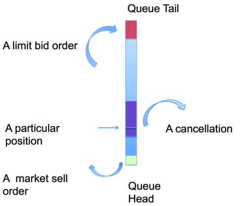
Figure 1: Orders happened in the best bid queue.

Our contributions.

The dynamics of an order position in a queue will be affected by both the market orders and the cancellations, and the dynamics of its relative position in a queue will be affected by the limit orders as well (see Figure 1). Without loss of generality, we will focus on an order position in the best bid queue along with the best bid and ask queues. Order positions in other queues will be similar and simpler because of the absence of market orders.

First, we derive the fluid limit for the order positions and related best bid and ask queues; in a sense, this is a first order approximation to the processes. We show (Theorem 11 and Theorem 31) that the rate of the order position approaching zero is proportional to the mean of order arrival intensities and to the summation of the average size of market orders and the “modified” average size of cancellation orders in the queue; this modification depends on different assumptions on order cancellations. We also derive the (average) time it takes for the order position to be executed. The derivation is via two steps. The first step is to establish the functional strong law of large numbers for the related bid/ask queues; this is straightforward. The second step is intuitive but requires a delicate analysis involving passing the convergence relation of stochastic processes in their corresponding càdlàg space with the Skorokhod topology to their integral equations.

Next, we proceed to the second order approximation for order positions and related queues. The first step is to establish appropriate forms of the diffusion limit for the bid and ask queues. We establish a multi-variate functional central limit theorem (FCLT) using ideas from random fields. Under appropriate technical conditions, we show (Theorem 14) that the queues are two-dimensional Brownian motion with mean and covariance structure explicitly given in terms of the statistics of order sizes and order arrival intensities. The second step is to combine the FCLTs and the fluid limit results to show (Theorem 15) that fluctuations of the order positions are Gaussian processes with “mean-reversion”. The mean-reverting level is essentially the fluid limit of order position relative to the queue length modified by the order book net flow, which is defined as the limit order minus the market order and the cancellation. The speed of the mean-reversion is proportional to the order arrival intensity and the rate of cancellations.

Our results are built on fairly general technical assumptions (stationarity and ergodicity) on order arrival processes and order sizes. For instance, order arrival processes (Section 4) can be Poisson processes or Hawkes processes, both of which have been extensively used in LOB modelings; see for instance, Abergel and Jedidi [2] and Huang, Lehalle, and Rosenbaum [33].

Practically speaking, studying order positions gives more direct estimates for the “value” of order positions, which is useful in algorithmic trading. Indeed, based on the fluid limit, we derive (Section 4) explicit analytical comparisons between the average time an order is executed and the average time any related queue is depleted. This is an important piece of information especially when combined with an estimate on the probability of a price increase. The latter is a core quantity for the LOB and has been studied in Avellaneda and Stoikov [6] and Cont and de Larrard [20, 19] for special cases. In addition, we derive from the fluctuation analysis explicit expressions for the first hitting times of the queue depletion, for the expected order execution time, and for the fluctuations of order execution time and first hitting times. Furthermore, by the large deviations theory, we derive the tail probability that the queues deviate from their fluid limits.

Related work.

The main idea behind our analysis is to draw connections between LOBs and multi-class priority queues, as LOBs with cancellations are reminiscent of reneging queues; see for instance Ward and Glynn [51, 52]. In the mathematical finance literature, there have been a number of papers on modeling LOB dynamics in a queuing framework and establishing appropriate diffusion and fluid limits for queue lengths or the order book prices. This line of work can be traced back to Kruk [39], who established diffusion and fluid limits for prices in an auction setting and showed that the best bid and ask queues converge to reflected two-dimensional Brownian motion in the first quadrant. Similar results were later obtained by Cont and de Larrard [19] for the best bid and best ask queues under heavy traffic conditions, where they also established the diffusion limit for the price dynamics under the same “reduced form” approach with stationary conditions on the queue lengths [20]. Abergel and Jedidi [1] modeled the volume of the order book by a continuous-time Markov chain with independent Poisson order flow processes and showed that mid price has a diffusion limit and that the order book is ergodic. Horst and Paulsen [32] studied the fluid limit for the whole limit order books including both prices and volumes, under a very general mathematical setting. Their analysis was further extended in Horst and Kreher [31], where the order dynamics could depend on the state of the LOB. Under different time and space scalings, Blanchet and Chen [9] derived a pure jump limit for the price-per-trade process and a jump diffusion limit for the price-spread process.

One of our results, Theorem 14, is mostly related to yet different from the diffusion limit in  [19]. This is a result of a different scaling approach. In order for us to analyze the dynamics of the order positions, we need to differentiate limit orders from market and cancellation orders, whereas in [19] order processes are aggregated from limit, market, and cancellations orders. Because of this aggregation, they could use the main idea from “heavy-traffic-limit” in classical queuing theory and assume that the mean order flow is dominated by the variance. While this assumption [19, Assumption 3.2] is critical to their analysis, it does not hold in our setting where each individual order type is considered. On the other hand, if we were to impose this assumption, then our result will be reduced to theirs because the second term in Eqn. (3.7) would simply vanish.

To the best of our knowledge, the dynamics of order positions and its relation to the queue lengths, which is the focus of our work, has not been studied before. Indeed, classical queuing tends to focus more on the stability of the entire system, rather than analyzing individual requests. Most of the existing modeling approaches in algorithmic trading have ignored order positions, with very limited efforts on the probability of it being executed. For instance, such a probability is either assumed to be a constant as in Cont and de Larrard [19, 20] and Guo, de Larrard and Ruan [29], or is computed numerically from modeling the whole LOB as a Markov chain as in Hult and Kiessling [34], or is analyzed with a homogeneous Poisson process for order arrivals and with constant order sizes as in Cont, Stoikov, and Talreja [22].

2 Fluid limits of order positions and related queues

2.1 Notation

Without loss of generality, consider the best bid and ask queues. Then there are six types of orders: best bid orders ($\mathsf{bb}$), market orders at the best bid ($\mathsf{mbb}$), cancellation at the best bid ($\mathsf{cbb}$), best ask ($\mathsf{ba}$), market orders at the best ask ($\mathsf{mba}$), and cancellation at the best ask ($\mathsf{cba}$). Denote the order arrival process by $\mathbf{N}=(N(t),t\geq 0)$ with the inter-arrival times $\{D_{i}\}_{i\geq 1}$. Here

$$N(t) = \max\left\{m:\sum_{i=1}^{m}D_{i}\leq t\right\}.$$

For simplicity, assume that there are no simultaneous arrivals of different types of orders. Consider order arrivals of any of these six types as a point process, and define a sequence of six-dimensional random vectors $\{\overrightarrow{V}_{i}\}_{i\geq 1}$, where for the $i$th order

$$\overrightarrow{V}_{i}=(V_{i}^{\mathsf{bb}},V_{i}^{\mathsf{mbb}},V_{i}^{\mathsf{cbb}},V_{i}^{\mathsf{ba}},V_{i}^{\mathsf{mba}},V_{i}^{\mathsf{cba}}):=(V_{i}^{1},V_{i}^{2},\ldots,V_{i}^{6}),$$

represents the sizes of the six types of orders; by the assumption, exactly one entry of $\overrightarrow{V}_{i}$ is positive. For instance, $\overrightarrow{V}_{5}=(0,0,0,4,0,0)$ means the fifth order is of size $4$ and of type $\mathsf{ba}$, i.e., a limit order at the best ask. In this paper, we only consider càdlàg processes.

For ease of references in the main text, we will use the following notation.

• $D[0,T]$ is the space of one-dimensional càdlàg functions on $[0,T]$, while $D^{K}[0,T]$ is the space of $K$-dimensional càdlàg functions on $[0,T]$. Consequently, the convergence in this space is, unless otherwise specified, in the sense of the weak convergence in $D^{K}[0,T]$ equipped with $J_{1}$ topology;

• $L_{\infty}[0,T]$ is the space of functions $f:[0,T]\rightarrow\mathbb{R}^{K}$, equipped with the topology of uniform convergence;

• $\mathcal{AC}_{0}[0,T]$ is the space of functions $f:[0,T]\rightarrow\mathbb{R}^{K}$ that are absolutely continuous and $f(0)=0$;

• $\mathcal{AC}_{0}^{+}[0,T]$ is the space of non-decreasing functions $f:[0,T]\rightarrow\mathbb{R}^{K}$ that are absolutely continuous and $f(0)=0$.

Similarly, we define $D[0,\infty)$, $D^{K}[0,\infty)$, $L_{\infty}[0,\infty)$, $\mathcal{AC}_{0}[0,\infty)$, $\mathcal{AC}_{0}^{+}[0,\infty)$ for $T=\infty.$

2.2 Technical assumptions and preliminaries

In order to study the fluid limit for the order position and related queues, we will first need to impose some technical assumptions.

Assumption 1.

$\{D_{i}\}_{i\geq 1}$ is a stationary array of positive random variables with

$$\frac{D_{1}+D_{2}+\cdots+D_{i}}{i}\rightarrow\frac{1}{\lambda},\qquad\text{in probability}$$

as $i\to\infty$, where $\lambda$ is a positive constant.

Assumption 2.

$\{\overrightarrow{V}_{i}\}_{i\geq 1}$ is a stationary array of square-integrable random vectors with

$$\frac{\overrightarrow{V}_{1}+\overrightarrow{V}_{2}+\cdots+\overrightarrow{V}_{i}}{i}\rightarrow\overrightarrow{\bar{V}},\qquad\text{in probability}$$

as $i\to\infty$, where $\overrightarrow{\bar{V}}=(\bar{V}^{1},\bar{V}^{2},\ldots,\bar{V}^{6})$ is a constant vector.

Assumption 3.

$\{D_{i}\}_{i\geq 1}$ is independent of $\{\overrightarrow{V}_{i}\}_{i\geq 1}$ .

Now, we define a new process $\overrightarrow{\mathbf{C}}_{n}$ as follows,

$$\overrightarrow{C}_{n}(t)=\frac{1}{n}\sum_{i=1}^{N(nt)}\overrightarrow{V}_{i}.$$ (2.1)

We call such a process $\overrightarrow{\mathbf{C}}_{n}$ the scaled net order flow process.

Theorem 4.

Given Assumptions 1 and 2, for any $T>0$,

$$\overrightarrow{\mathbf{C}}_{n}\Rightarrow\lambda\overrightarrow{\bar{V}}\mathbf{e},\qquad\text{in $(D^{6}[0,T],J_{1})$ \ \ as $n\rightarrow\infty$},$$

where $\mathbf{e}$ is the identity function.

Proof.

First, we define the scaled processes $\mathbf{S}^{D}_{n}$ and $\overrightarrow{\mathbf{S}}^{V}_{n}$ by

$$S^{D}_{n}(t) =\frac{1}{n}\sum_{i=1}^{\lfloor nt\rfloor}D_{i},$$

$$\overrightarrow{S}^{V}_{n}(t) =\frac{1}{n}\sum_{i=1}^{\lfloor nt\rfloor}\overrightarrow{V}_{i}.$$

Then by Assumption 1 and according to Glynn and Whitt [25, Theorem 5], the strong Law of Large Numbers (SLLN) also follows, i.e.,

$$\lim\limits_{i\to\infty}\frac{D_{1}+D_{2}+\cdots+D_{i}}{i}=\frac{1}{\lambda},\qquad\text{a.s.}$$

Then by the equivalence of SLLN and FSLLN [25, Theorem 4], it is clear that for any $T>0$,

$$\mathbf{S}_{n}^{D}=\frac{1}{n}\sum_{i=1}^{\lfloor n\cdot\rfloor}D_{i}\Rightarrow\frac{\mathbf{e}}{\lambda},\qquad\text{a.s. in $(D[0,T],J_{1})$ as $n\rightarrow\infty$}.$$

Moreover, since $\overrightarrow{V}_{1}$ is square-integrable, it follows that $\mathbb{E}[V^{j}_{1}]<\infty$ for $1\leq j\leq 6$. Note that $\{V^{j}_{i}\}_{i\geq 1}$ is stationary and applying Birkhoff’s Ergodic Theorem [11, Theorem 6.28] leads to

$$\frac{1}{n}\sum_{i=1}^{n}V^{j}_{i}\rightarrow\mathbb{E}[V_{1}^{j}\mid\mathcal{I}^{j}],\qquad\text{a.s. as $n\rightarrow\infty$,}$$

where $\mathcal{I}^{j}$ is the invariant $\sigma$-algebra of $\{V_{i}^{j}\}_{i\geq 1}$. Given the WLLN for $\{V_{i}^{j}\}_{i\geq 1}$, it follows that

$$\mathbb{E}[V_{1}^{j}\mid\mathcal{I}^{j}]=\bar{V}^{j},$$

and

$$\frac{1}{n}\sum_{i=1}^{n}V^{j}_{i}\rightarrow\bar{V}^{j},\qquad\text{a.s. as $n\rightarrow\infty$.}$$

Therefore, again by [25, Theorem 4],

$$\overrightarrow{\mathbf{S}}_{n}^{V,j}=\frac{1}{n}\sum_{i=1}^{\lfloor n\cdot\rfloor}V_{i}^{j}\Rightarrow\bar{V}^{j}\mathbf{e},\qquad\text{a.s. in $(D[0,T],J_{1})$ as $n\rightarrow\infty$}$$

Since the limit processes for $\{\mathbf{S}_{n}^{D}\}_{n\geq 1}$ and $\{\mathbf{S}_{n}^{V,j}\}_{n\geq 1}$, $1\leq j\leq 6$, are deterministic, then according to [53, Theorem 11.4.5],

$$(\overrightarrow{\mathbf{S}}_{n}^{V},\mathbf{S}_{n}^{D})\Rightarrow\left(\overrightarrow{\bar{V}}\mathbf{e},\frac{\mathbf{e}}{\lambda}\right),\qquad\text{a.s. in $(D^{7}[0,T],J_{1})$ as $n\rightarrow\infty$}.$$

Finally, from [53, Theorem 9.3.4],

$$\overrightarrow{\mathbf{C}}_{n}\Rightarrow\lambda\overrightarrow{\bar{V}}\mathbf{e},\enspace\mbox{in }(D^{6}[0,T],J_{1})\mbox{ as }n\rightarrow\infty.\qquad\hfill\qed$$

Next we proceed to study the order position in the best bid and related queues of the best bid and the best ask. We further assume

Assumption 5.

Cancellations are uniformly distributed on every queue.

We will see that this assumption on cancellation is not critical, except for affecting the exact form of the fluid limit for the order position. (See Theorem 31 without this assumption in Section 5.)

Now define the scaled queue lengths with $\mathbf{Q}_{n}^{b}$ for the best bid queue and $\mathbf{Q}_{n}^{a}$ for the best ask queue, and the scaled order position $\mathbf{Z}_{n}$ by

$$\left\{\begin{aligned} Q_{n}^{b}(t)&=Q_{n}^{b}(0)+C^{1}_{n}(t)-C^{2}_{n}(t)-C^{3}_{n}(t),\\ Q_{n}^{a}(t)&=Q_{n}^{a}(0)+C^{4}_{n}(t)-C^{5}_{n}(t)-C^{6}_{n}(t),\\ dZ_{n}(t)&=-dC^{2}_{n}(t)-\frac{Z_{n}(t-)}{Q_{n}^{b}(t-)}dC^{3}_{n}(t).\end{aligned}\right.$$ (2.2)

The above equations are straightforward: bid/ask queue lengths increase with limit orders and decrease with market orders and cancellations according to their corresponding order flow processes; an order position will decrease and move towards zero with arrivals of cancellations and market orders; new limit orders arrivals will not change this particular order position; however, the arrival of limit orders may change the speed of the order position approaching zero following Assumption 5, hence the factor of $\frac{Z_{n}(t-)}{Q_{n}^{b}(t-)}$.

Strictly speaking, Eqn. (2.2) only describes the dynamics of the triple $(Q_{n}^{b}(t),Q_{n}^{a}(t),Z_{n}(t))$ before any of them hits zero: $\mathbf{Z}_{n}$ hitting zero means that the order placed has been executed, while $\mathbf{Q}_{n}^{a}$ hitting zero means that the best ask queues is depleted. Since our primary interest is in the order position, with little risk we may truncate the processes to avoid unnecessary technical difficulties on the boundary. That is, define

$$\tau_{n}=\min\{\tau_{n}^{z},\tau_{n}^{a},\tau_{n}^{b}\},$$ (2.3)

with

$$\tau_{n}^{b}=\inf\{t\geq 0:Q_{n}^{b}(t)\leq 0\},\qquad\tau_{n}^{a}=\inf\{t\geq 0:Q_{n}^{a}(t)\leq 0\},\qquad\tau_{n}^{z}=\inf\{t\geq 0:Z_{n}(t)\leq 0\}.$$

Now, define the truncated processes

$$\tilde{Q}_{n}^{b}(t)=Q_{n}^{b}(t\wedge\tau_{n}),\qquad\tilde{Q}_{n}^{a}(t)=Q_{n}^{a}(t\wedge\tau_{n}),\qquad\tilde{Z}_{n}(t)=Z_{n}(t\wedge\tau_{n}).$$ (2.4)

Still, it is not immediately clear that these truncated processes would be well defined either since we do not know a priori if the term $-\frac{Z_{n}(t-)}{Q_{n}^{b}(t-)}$ is bounded when $\mathbf{Q}_{n}^{b}$ hits zero. This, however, turns out not to be an issue.

Lemma 6.

Eqn. (2.4) is well defined, with $Z_{n}(t)\leq Q_{n}^{b}(t)$ for any time $t\leq\min(\tau_{n}^{z},\tau_{n}^{a})$. In particular, $\tau_{n}^{z}\leq\tau_{n}^{b}$.

Proof.

Note that $\overrightarrow{\mathbf{C}}_{n}$ is a positive jumping process. Therefore, when $\delta Z_{n}(t)=0$, we have $\delta C^{1}_{n}(t)>0$ and $\delta Q_{n}^{b}(t)>0$; when $\delta C^{2}_{n}(t)>0$, we have $\delta Q_{n}^{b}(t)=\delta Z_{n}(t)$; and when $\delta C^{3}_{n}(t)>0$, we have $\frac{\delta Q_{n}^{b}(t)}{Q_{n}^{b}(t-)}=\frac{\delta Z_{n}(t)}{Z_{n}(t-)}$. Hence, when $0<Z_{n}(t-)\leq Q_{n}^{b}(t-)$, we have $Z_{n}(t)\leq Q_{n}^{b}(t)$. Moreover, the number of order arrivals for any given time horizon is finite with probability 1. ∎

This lemma, though simple, turns out to play an important role to ensure that fluid limits of order positions and related queues are well defined after rescaling. That is, we can extend the definition of $\tilde{\mathbf{Q}}_{n}^{b}$, $\tilde{\mathbf{Q}}_{n}^{a}$, and $\tilde{\mathbf{Z}}_{n}$ for any time $t\geq 0$.

For simplicity, for the rest of the paper we will use $\mathbf{Q}_{n}^{b}$, $\mathbf{Q}_{n}^{a}$, and $\mathbf{Z}_{n}$ instead of $\tilde{\mathbf{Q}}_{n}^{b}$, $\tilde{\mathbf{Q}}_{n}^{a}$, and $\tilde{\mathbf{Z}}_{n}$, defined on $t\geq 0$. The dynamics of the truncated processes could be described in the following matrix form.

$$d\left(\begin{aligned} &{Q}_{n}^{b}(t)\\ &{Q}_{n}^{a}(t)\\ &{Z}_{n}(t)\end{aligned}\right) =\left(\begin{array}[]{cccccc}1&-1&-1&0&0&0\\ 0&0&0&1&-1&-1\\ 0&-1&-\frac{{Z}_{n}(t-)}{{Q}_{n}^{b}(t-)}&0&0&0\end{array}\right)\mathbb{I}_{{Q}_{n}^{a}(t-)>0,Q_{n}^{b}(t-)>0,{Z}_{n}(t-)>0}\cdot d\overrightarrow{C}_{n}(t).$$ (2.8)

The modified processes coincide with the original processes before hitting zero, which implies $\mathbb{I}_{t\leq\tau_{n}}=\mathbb{I}_{{Q}_{n}^{a}(t-)>0,Q_{n}^{b}(t-)>0,{Z}_{n}(t-)>0}$.

In order to establish the fluid limit for the joint process ($\mathbf{Q}_{n}^{b}$, $\mathbf{Q}_{n}^{a}$ and $\mathbf{Z}_{n}$), we see that it is fairly standard to establish the limit process for $(\mathbf{Q}_{n}^{b},\mathbf{Q}_{n}^{a})$ from classical probability theory where various forms of functional strong law of large numbers exist. However, checking Eqn. (2.8) for $Z_{n}(t)$, we see that in order to pass from the fluid limit for $\mathbf{Q}_{n}^{b}$ to that for $\mathbf{Z}_{n}(t)$, we effectively need to pass the convergence relation between some càdlàg processes $(\mathbf{X}_{n},\mathbf{Y}_{n})$ to $(\mathbf{X},\mathbf{Y})$ in the Skorokhod topology to the convergence relation between $\int X_{n}dY_{n}$ to $\int XdY$. That is, consider a sequence of stochastic processes $\{\mathbf{X}_{n}\}_{n\geq 1}$ defined by a sequence of SDEs

$$X_{n}(t)=U_{n}(t)+\int_{0}^{t}F_{n}(X_{n},s-)dY_{n}(s),$$ (2.9)

where $\{\mathbf{U}_{n}\}_{n\geq 1}$, $\{\mathbf{Y}_{n}\}_{n\geq 1}$ are two sequences of stochastic processes and $\{F_{n}\}_{n\geq 1}$ is a sequence of functionals. Now, suppose that $\{\mathbf{U}_{n},\mathbf{Y}_{n},F_{n}\}_{n\geq 1}$ converges to $\{\mathbf{U},\mathbf{Y},F\}$ in some way. Then, would the sequence of the solutions to Eqn. (2.9) converge to the solution to

$$X(t)=U(t)+\int_{0}^{t}F(X,s-)dY(s)?$$

It turns out that such a convergence relation is delicate and can easily fail, as shown by the following simple example.

Example 7.  Let $\{X_{i}\}_{i\geq 1}$ be a sequence of identically distributed random variables taking values in $\{-1,1\}$ such that

$$\mathbb{P}(X_{1}=1)=\mathbb{P}(X_{1}=-1)=\frac{1}{2},\quad\mathbb{P}(X_{i+1}=1\mid X_{i}=1)=\mathbb{P}(X_{i+1}=-1\mid X_{i}=-1)=\frac{3}{4}\mbox{ for }i>1.$$

Define $S_{n}(t)=\frac{1}{\sqrt{n}}\sum_{i=1}^{\lfloor nt\rfloor}X_{i}$. Note that $\{X_{i}\}_{i\geq 1}$ is a strictly stationary sequence, with mean zero and is a Markov Chain with finite state space $\{-1,1\}$. Since each entry of the transition probability matrix is strictly between $0$ and $1$, the sequence $\{X_{i}\}_{i\geq 1}$ is $\psi$-mixing, see e.g., [46]. Note that $\psi$-mixing implies $\phi$-mixing, see e.g., [10]. By stationarity,

$$\lim_{n\rightarrow\infty}\frac{1}{n}\mathbb{E}\left[\left(\sum_{i=1}^{n}X_{i}\right)^{2}\right]=\sigma^{2}=\mathbb{E}[X_{1}^{2}]+2\sum_{i=1}^{\infty}\mathbb{E}[X_{1}X_{i+1}].$$

We can compute by induction that for any $i\geq 1$,

$$\mathbb{E}[X_{1}X_{i+1}]=\frac{3}{4}\mathbb{E}[X_{1}X_{i}]+\frac{1}{4}\mathbb{E}[X_{1}(-X_{i})]=\frac{1}{2}\mathbb{E}[X_{1}X_{i}]=\frac{1}{2^{i}}.$$

Therefore, we have $\sigma^{2}=1+2\sum_{i=1}^{\infty}\frac{1}{2^{i}}=3.$ For strictly stationary centered $\phi$-mixing sequence with $\mathbb{E}\left[\left(\sum_{i=1}^{n}X_{i}\right)^{2}\right]\rightarrow\infty$ as $n\rightarrow\infty$ and $\mathbb{E}[|X_{1}|^{2+\delta}]<\infty$ for some $\delta>0$, the invariance principle holds, see e.g., [35], i.e., $\mathbf{S}_{n}$ converges to $\sigma\mathbf{B}$. Hence $\mathbf{S}_{n}$ converges to $\sqrt{3}\mathbf{B}$. Now define a sequence of SDE’s $dY_{n}(t)=Y_{n}(t)dS_{n}(t)$ with $Y_{n}(0)=1.$ Clearly, since $X_{i}\in\{\pm 1\}$ and $|X_{i}|\leq 1$, for sufficiently large $n$,

$$Y_{n}(t)=\prod_{i=1}^{\lfloor nt\rfloor}\left(1+\frac{X_{i}}{\sqrt{n}}\right)=e^{\sum_{i=1}^{\lfloor nt\rfloor}\log(1+\frac{X_{i}}{\sqrt{n}})}=e^{\frac{1}{\sqrt{n}}\sum_{i=1}^{\lfloor nt\rfloor}X_{i}-\frac{1}{2n}\lfloor nt\rfloor+\epsilon_{n}},$$

where $|\epsilon_{n}|\leq\frac{C}{\sqrt{n}}$, where $C>0$ is a constant. Hence, $\mathbf{Y}_{n}$ converges to the limiting process described by $\exp\{\sqrt{3}B(t)-\frac{t}{2}\}$, as $n\to\infty$. However, the solution to $dY(t)=Y(t)d(\sqrt{3}B(t))$ with $Y(0)=1$ is given by $Y(t)=\exp\{\sqrt{3}B(t)-\frac{3t}{2}\}$. $\clubsuit$

Nevertheless, under proper conditions as specified in Assumptions 1, 2, 5, one can establish the desired convergence relation. Such assumptions prove to be sufficient using a result of Kurtz and Protter [40, Theorem 5.4]. For sake of completeness, we present this result next, along with the technical conditions required for the convergence.

2.3 Detour: Convergence of stochastic processes by Kurtz and Protter [40]

Define $h_{\delta}(r):[0,\infty)\to[0,\infty)$ by $h_{\delta}(r)=(1-\delta/r)^{+}$. Define $J_{\delta}:D^{m}[0,\infty)\to D^{m}[0,\infty)$ by

$$J_{\delta}(x)(t)=\sum_{s\leq t}h_{\delta}(|x(s)-x(s-)|)(x(s)-x(s-)).$$

Let ${Y_{n}}$ be a sequence of stochastic processes adapted to ${\mathcal{F}_{t}}$. Define $Y_{n}^{\delta}=Y_{n}-J_{\delta}(Y_{n})$. Let $Y_{n}^{\delta}=M_{n}^{\delta}+A_{n}^{\delta}$ be a decomposition of $Y_{n}^{\delta}$ into an ${\mathcal{F}_{t}}$-local martingale and a process with finite variation.

Condition 8.

For each $\alpha>0$, there exist stopping times ${\tau_{n}^{\alpha}}$ such that $P\{\tau_{n}^{\alpha}\leq 1\}\leq 1/\alpha$ and $\sup_{n}\mathbb{E}[[M_{n}^{\delta}]_{t\leq\tau_{n}^{\alpha}}+T(A_{n}^{\delta})_{t\leq\tau_{n}^{\alpha}}]<\infty$, where $[M_{n}^{\delta}]_{t\leq\tau_{n}^{\alpha}}$ denotes the total quadratic variation of $M_{n}^{\delta}$ up to time $\tau_{n}^{\alpha}$, and $T(A_{n}^{\delta})_{t\leq\tau_{n}^{\alpha}}$ denotes the total variation of $A_{n}^{\delta}$ up to time $\tau_{n}^{\alpha}$.

Let $T_{1}[0,\infty)$ denote the collection of non-decreasing mappings $\lambda$ of $[0,\infty)$ to $[0,\infty)$ (in particular, $\lambda(0)=0$) such that $\lambda(h+t)-\lambda(t)\leq h$ for all $t,h\geq 0$. Let $\mathbb{M}^{km}$ be the space of real-valued $k\times m$ matrices, and $D_{\mathbb{M}^{km}}[0,\infty)$ be the space of càdlàg functions from $[0,\infty)$ to $\mathbb{M}^{km}$. Assume that there exist mappings $G_{n},G:D^{k}[0,\infty)\times T_{1}[0,\infty)\to D_{\mathbb{M}^{km}}[0,\infty)$ such that $F_{n}\circ\lambda=G_{n}(x\circ\lambda,\lambda)$ and $F(x)\circ\lambda=G(x\circ\lambda,\lambda)$ for $(x,\lambda)\in D^{k}[0,\infty)\times T_{1}[0,\infty)$.

Condition 9.

(i) For each compact subset $\mathcal{H}\subset D^{k}[0,\infty)$ and $t>0$, $\sup_{(x,\lambda)\in\mathcal{H}}\sup_{s\leq t}|G_{n}(x,\lambda,s)-G(x,\lambda,s)|\to 0$;

(ii) For $\{(x_{n},\lambda^{n})\}\in D^{k}[0,\infty)\times T_{1}[0,\infty)$, $\sup_{s\leq t}|x_{n}(s)-x(s)|\to 0$ and $\sup_{s\leq t}|\lambda^{n}(s)-\lambda(s)|\to 0$ for each $t>0$ implies $\sup_{s\leq t}|G(x_{n},\lambda^{n},s)-G(x,\lambda,s)|\to 0$.

Theorem 10.

Suppose that $(\mathbf{U}_{n},\mathbf{X}_{n},\mathbf{Y}_{n})$ satisfies

$$X_{n}(t)=U_{n}(t)+\int_{0}^{t}F_{n}(X_{n},s-)dY_{n}(s),$$

$(\mathbf{U}_{n},\mathbf{Y}_{n})\Rightarrow(\mathbf{U},\mathbf{Y})$ in the Skorokhod topology, and that $\{\mathbf{Y}_{n}\}$ satisfies Condition 8 for some $0<\delta\leq\infty$. Assume that $\{F_{n}\}$ and $F$ have representations in terms of $\{G_{n}\}$ and $G$ satisfying Condition 9. If there exists a global solution $X$ of

$$dX(t)=U(t)+\int_{0}^{t}F(X,s-)dY(s),$$

and the local uniqueness holds, then

$$(\mathbf{U}_{n},\mathbf{X}_{n},\mathbf{Y}_{n})\Rightarrow(\mathbf{U},\mathbf{X},\mathbf{Y}).$$

2.4 Fluid limit for order positions and related queues

We are now ready to establish our first result.

Theorem 11.

Given Assumptions 1, 2, 3, and 5, suppose there exist constants $q^{b}$, $q^{a}$, and $z$ such that

$$(Q_{n}^{b}(0),Q_{n}^{a}(0),Z_{n}(0))\Rightarrow(q^{b},q^{a},z).$$

Then, for any $T>0$, Eqn. (2.8)

$$({\mathbf{Q}}_{n}^{b},{\mathbf{Q}}_{n}^{a},{\mathbf{Z}}_{n})\Rightarrow({\mathbf{Q}}^{b},{\mathbf{Q}}^{a},{\mathbf{Z}})\qquad\text{in}\quad(D^{3}[0,T],J_{1}),$$

where $({\mathbf{Q}}^{b},{\mathbf{Q}}^{a},{\mathbf{Z}})$ is given by

$${Q}^{b}(t)=q^{b}-\lambda v^{b}(t\wedge\tau),$$ (2.10)

$${Q}^{a}(t)=q^{a}-\lambda v^{a}(t\wedge\tau),$$ (2.11)

and for $t<\tau$,

$$\frac{d{Z}(t)}{dt}=-\lambda\left(\bar{V}^{2}+\bar{V}^{3}\frac{{Z}(t-)}{{Q}^{b}(t-)}\right),\qquad{Z}(0)=z.$$ (2.12)

Here $\tau=\min\{\tau^{a},\tau^{b},\tau^{z}\}$ with

$$\tau^{a}=\frac{q^{a}}{\lambda v^{a}},\qquad\qquad\tau^{b}=\frac{q^{b}}{\lambda v^{b}},$$ (2.13)

and

$$\tau^{z}=\left\{\begin{aligned} &\left(\frac{(1+c)z}{a}+b\right)^{c/(c+1)}b^{1/(c+1)}c^{-1}-b/c\qquad&\qquad c\notin\{-1,0\},\\ &b(1-e^{-\frac{z}{ab}})\qquad&\qquad c=-1,\\ &b\log\left(\frac{z}{ab}+1\right)&\qquad c=0.\end{aligned}\right.$$ (2.14)

Moreover, if $v^{b}>0$, $v^{a}>0$, and $q^{a}/v^{a}>q^{b}/v^{b},$ then $\tau_{n}^{z}\rightarrow\tau^{z}$ a.s. as $n\rightarrow\infty$, where

$$a=\lambda\bar{V}^{2},\quad b=q^{b}/(\lambda\bar{V}^{3}),\quad c=-\frac{v^{b}}{\bar{V}^{3}},$$ (2.15)

$$v^{b}=-\bar{V}^{1}+\bar{V}^{2}+\bar{V}^{3},\ \ v^{a}=-\bar{V}^{4}+\bar{V}^{5}+\bar{V}^{6}.$$ (2.16)

Proof.

Note that Eqns. (2.10), (2.11), (2.12) satisfy the following SDE’s

$$d\left(\begin{aligned} &{Q}^{b}(t)\\ &{Q}^{a}(t)\\ &{Z}(t)\end{aligned}\right)= \left(\begin{array}[]{cccccc}1&-1&-1&0&0&0\\ 0&0&0&1&-1&-1\\ 0&-1&-\frac{{Z}(t-)}{{Q}^{b}(t-)}&0&0&0\end{array}\right)\mathbb{I}_{{Q}^{a}(t-)>0,{Q}^{b}(t-)>0,{Z}(t-)>0}\lambda\overrightarrow{\bar{V}}dt;$$ (2.20)

$$({Q}^{b}(0),{Q}^{a}(0),{Z}(0))= (q^{b},q^{a},z).$$

Therefore, we first show the convergence to Eqn. (2.20). Now, set $Y_{n}=\overrightarrow{\mathbf{C}}_{n}$, $X_{n}=({\mathbf{Q}}_{n}^{b},{\mathbf{Q}}^{a}_{n},{\mathbf{Z}}_{n})$, and

$$F_{n}(x,s-)=F(x,s-)=\left(\begin{aligned} 1&\quad-1&-1&\quad 0&\quad 0&\quad 0&\\ 0&\qquad 0&0&\quad 1&\quad-1&\quad-1&\\ 0&\quad-1&\quad-\frac{x^{3}(s-)}{x^{1}(s-)}&\quad 0&\quad 0&\quad 0&\end{aligned}\right)\mathbb{I}_{x(s-)>0}.$$

In order to apply Theorem 10, we need to decompose $Y_{n}$. Now take $\delta=\infty$, define the filtrations $\mathcal{F}^{n}_{t}:=\sigma(\{N(s)\}_{0\leq s\leq nt},\{\overrightarrow{V}_{i}\}_{1\leq i\leq N(nt)})$ and $\mathcal{G}_{i}:=\sigma(\{\overrightarrow{V}_{k}\}_{1\leq k\leq i})$,

$$M_{n}(t)=\frac{1}{n}\sum_{i=1}^{N(nt)}\overrightarrow{V}_{i}-\mathbb{E}[\overrightarrow{V}_{i}\mid\mathcal{G}_{i-1}],$$

and

$$A_{n}(t)=Y_{n}(t)-M_{n}(t).$$

We will show that $M_{n}$ is a martingale with respect to $\mathcal{F}^{n}_{t}$ and $\{Y_{n}\}_{n\geq 1}$ satisfies Condition 8 in Theorem 10.

For $s\in[0,t)$, it is easy to see that Assumption 3 implies that $\mathbb{E}[\overrightarrow{V}_{i}\mid\mathcal{F}^{n}_{\frac{1}{n}\sum_{k=1}^{i-1}D_{k}}]=\mathbb{E}[\overrightarrow{V}_{i}\mid\mathcal{G}_{i-1}]$. Thus

$$\mathbb{E}\left[\mathbb{E}\left[\overrightarrow{V}_{i}\mid\mathcal{G}_{i-1}\right]\big{|}\mathcal{F}^{n}_{s}\cap(N(ns)<i)\right]$$

$$=\mathbb{E}\left[\mathbb{E}\left[\overrightarrow{V}_{i}\mid\mathcal{F}^{n}_{\frac{1}{n}\sum_{k=1}^{i-1}D_{k}}\right]\Big{|}\mathcal{F}^{n}_{s}\cap(N(ns)<i)\right]$$

$$=\mathbb{E}\left[\overrightarrow{V}_{i}\big{|}\mathcal{F}^{n}_{s}\cap(N(ns)<i)\right].$$

Meanwhile, $\mathcal{F}^{n}_{\frac{1}{n}\sum_{k=1}^{i}D_{k}}\cap(N(ns)\geq i)\subseteq\mathcal{F}^{n}_{s}\cap(N(ns)\geq i)$. Thus

$$\mathbb{E}\left[\mathbb{E}\left[\overrightarrow{V}_{i}\mid\mathcal{G}_{i-1}\right]\Big{|}\mathcal{F}^{n}_{s}\cap(N(ns)\geq i)\right]$$

$$=\mathbb{E}\left[\mathbb{E}\left[\overrightarrow{V}_{i}\mid\mathcal{F}^{n}_{\frac{1}{n}\sum_{k=1}^{i}D_{k}}\right]\Big{|}\mathcal{F}^{n}_{s}\cap(N(ns)\geq i)\right]$$

$$=\mathbb{E}\left[\overrightarrow{V}_{i}\big{|}\mathcal{F}^{n}_{\frac{1}{n}\sum_{k=1}^{i}D_{k}}\cap(N(ns)\geq i)\right]$$

$$=\mathbb{E}\left[\overrightarrow{V}_{i}\mid\mathcal{G}_{i-1}\cap(N(ns)\geq i)\right].$$

Moreover, $\mathbb{E}\left[\overrightarrow{V}_{i}\big{|}\mathcal{F}^{n}_{s}\cap(N(ns)\geq i)\right]=\overrightarrow{V}_{i}$ since $\overrightarrow{V}_{i}$ is measurable with respect to $\mathcal{F}^{n}_{s}\cap(N(ns)\geq i)$. Therefore,

$$\mathbb{E}\left[M_{n}(t)\big{|}\mathcal{F}^{n}_{s}\right] =\mathbb{E}\left[\sum_{i=1}^{N(nt)}\frac{\overrightarrow{V}_{i}-\mathbb{E}[\overrightarrow{V}_{i}\mid\mathcal{G}_{i-1}]}{n}\bigg{|}\mathcal{F}^{n}_{s}\right]$$

$$=\frac{1}{n}\sum_{i=1}^{N(ns)}\left(\mathbb{E}\left[\overrightarrow{V}_{i}\mid\mathcal{F}^{n}_{s}\cap(N(ns)\geq i)\right]-\mathbb{E}\left[\mathbb{E}[\overrightarrow{V}_{i}\mid\mathcal{G}_{i-1}\cap(N(ns)\geq i)]\Big{|}\mathcal{F}^{n}_{s}\right]\right)$$

$$\quad+\frac{1}{n}\mathbb{E}\left[\sum_{i=N(ns)+1}^{N(nt)}\overrightarrow{V}_{i}-\mathbb{E}[\overrightarrow{V}_{i}\mid\mathcal{G}_{i-1}]\bigg{|}\mathcal{F}^{n}_{s}\cap(N(ns)<i)\right]$$

$$=\frac{1}{n}\sum_{i=1}^{N(ns)}\left(\overrightarrow{V}_{i}-\mathbb{E}[\overrightarrow{V}_{i}\mid\mathcal{G}_{i-1}\cap(N(ns)\geq i)]\right)$$

$$\quad+\frac{1}{n}\lambda n(t-s)\Big{(}\mathbb{E}[\overrightarrow{V}_{i}\big{|}\mathcal{F}^{n}_{s}\cap(N(ns)<i)]-\mathbb{E}\left[\mathbb{E}[\overrightarrow{V}_{i}\mid\mathcal{G}_{i-1}]\Big{|}\mathcal{F}^{n}_{s}\cap(N(ns)<i)\right]\Big{)}$$

$$=\frac{1}{n}\sum_{i=1}^{N(ns)}\left(\overrightarrow{V}_{i}-\mathbb{E}[\overrightarrow{V}_{i}\mid\mathcal{G}_{i-1}\cap(N(ns)\geq i)]\right)=M_{t}(s).$$

And $\mathbb{E}|M_{n}(t)|<\infty$ follows directly from Assumption 2. Hence it follows that $M_{n}(t)$ is a martingale. The quadratic variance of $M_{n}(t)$ is as follows:

$$\mathbb{E}\big{[}[M_{n}]_{t}\big{]} =\frac{nt}{n^{2}}\sum_{j=1}^{6}\mathbb{E}\left[\lambda\left(V^{j}_{i}-\mathbb{E}\left[V^{j}_{i}\big{|}\mathcal{G}_{i-1}\right]\right)^{2}\right]$$

$$=\frac{t}{n}\sum_{j=1}^{6}\lambda\mathbb{E}\left[\left(V^{j}_{i}\right)^{2}-2V^{j}_{i}\mathbb{E}\left[V^{j}_{i}\big{|}\mathcal{G}_{i-1}\right]+\left(\mathbb{E}\left[V^{j}_{i}\big{|}\mathcal{G}_{i-1}\right]\right)^{2}\right]$$

$$=\frac{t}{n}\sum_{j=1}^{6}\lambda\left(\mathbb{E}\left(V^{j}_{i}\right)^{2}-\mathbb{E}\left(\mathbb{E}\left[V^{j}_{i}\big{|}\mathcal{G}_{i-1}\right]\right)^{2}\right)\leq\frac{t}{n}\sum_{j=1}^{6}\lambda\mathbb{E}\left(V^{j}_{i}\right)^{2},$$

since

$$\mathbb{E}\left[V^{j}_{i}\mathbb{E}\left[V^{j}_{i}\big{|}\mathcal{G}_{i-1}\right]\right] =\mathbb{E}\left[\mathbb{E}\left[V^{j}_{i}\mathbb{E}\left[V^{j}_{i}\big{|}\mathcal{G}_{i-1}\right]\right]\Big{|}\mathcal{G}_{i-1}\right]=\mathbb{E}\left(\mathbb{E}\left[V^{j}_{i}\big{|}\mathcal{G}_{i-1}\right]\right)^{2}.$$

Thus $\mathbb{E}\left[[M_{n}]_{t}\right]$ is bounded uniformly in $n$ since $\overrightarrow{V}_{i}$ is square-integrable. Let $[T(A_{n})]_{t}$ denote the total variation of $A_{n}$ up to time $t$. Then $\mathbb{E}\left[[T(A_{n})]_{t}\right]$ is also uniformly bounded in $n$, as

$$\mathbb{E}\left[[T(A_{n})]_{t}\right] =t\sum_{j=1}^{6}\lambda\mathbb{E}\left|\mathbb{E}\left[V^{j}_{i}\big{|}\mathcal{G}_{i-1}\right]\right|\enspace\leq\enspace t\sum_{j=1}^{6}\lambda\mathbb{E}\left[\mathbb{E}\left[|V^{j}_{i}|\big{|}\mathcal{G}_{i-1}\right]\right]$$ (2.21)

$$=t\sum_{j=1}^{6}\lambda\mathbb{E}|V_{1}^{j}|\enspace<\enspace\infty,$$ (2.22)

where the inequality in Eqn. (2.21) uses the Jensen’s inequality for conditional expectations and Eqn. (2.22) follows from the square-integrability assumption. Thus, $Y_{n}$ satisfies Condition 8 with $\tau_{n}^{\alpha}=\alpha+1$. Moreover, taking $G_{n}(x\circ\mathbf{e},\mathbf{e})=F_{n}(x)=F(x)$, it is easy to see that Condition 9 is satisfied according to [40].

Now ${Q}^{a}(t)=0$ when $t=\tau^{a}$ as given in Eqn. (2.13); $\tau^{a}>0$ if $\bar{V}^{4}-\bar{V}^{5}-\bar{V}^{6}<0$; otherwise ${Q}^{a}(t)$ never hits zero in which case define $\tau^{a}=\infty$. The case for $\tau^{b}$ is similar.

It remains to find the unique solution for the limit Eqn. (2.20). The equation for $Z(t)$ when ${Z}(t-)>0$ is a first-order linear ODE with the solution

$${Z}(t)=\left\{\begin{aligned} &-\frac{a}{1+c}(b+c(t\wedge\tau))+\left(z+\frac{ab}{1+c}\right)\left(\frac{b}{b+c(t\wedge\tau)}\right)^{1/c}\qquad&\qquad c\notin\{-1,0\},\\ &(a\log(b-(t\wedge\tau))+z/b-a\log b)\cdot(b-(t\wedge\tau))\qquad&\qquad c=-1,\\ &(z+ab)e^{-t/b}-ab&\qquad c=0.\end{aligned}\right.$$ (2.23)

From the solution, we can solve $\tau^{z}$ explicitly as given in Eqn. (2.14). Note that the expression for ${Z}(t)$ may not be monotonic and there might be multiple roots when $c\neq 0$. Nevertheless, it is easy to check that the solution given in Eqn. (2.14) is the smallest positive root. For instance, when $c\notin\{-1,0\}$, there are two roots $-b/c$ and $\left(\frac{(1+c)z}{a}+b\right)^{c/(c+1)}b^{1/(c+1)}c^{-1}-b/c$ and when $c=-1$, there are two roots $b$ and $b(1-e^{-\frac{z}{ab}})$. More computations confirm that indeed the smallest positive roots are $\tau^{z}=\left(\frac{(1+c)z}{a}+b\right)^{c/(c+1)}b^{1/(c+1)}c^{-1}-b/c$ for $c\notin\{-1,0\}$ and $\tau^{z}=b(1-e^{-\frac{z}{ab}})$ for $c=-1$. Moreover, $\tau^{z}<\tau^{b}$ from these calculations. Therefore $\tau=\min\{\tau^{a},\tau^{z}\}$ is well defined and finite. ∎

The following figure illustrates the fluid limits of $(Q^{b}(t),Q^{a}(t),Z(t))$ with $Q^{b}(0)=Q^{a}(0)=Z(0)=100$, $\lambda=1$, $\bar{V}^{1}=\bar{V}^{4}=1$, $\bar{V}^{2}=0.6,\bar{V}^{3}=0.8,\bar{V}^{5}=0.7,\bar{V}^{6}=0.8$.

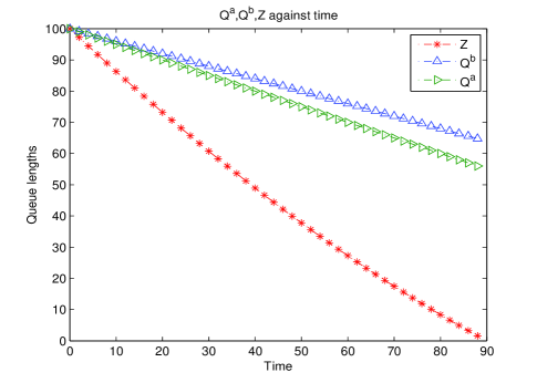
Figure 2: Illustration of the fluid limit$(Q^{b}(t),Q^{a}(t),Z(t))$.

3 Fluctuation analysis

The fluid limits in the previous section are essentially functional strong law of large numbers, and may well be regarded as the “first order” approximation for order positions and related queues. In this section, we will proceed to obtain a “second order” approximation for these processes. We will first derive appropriate diffusion limits for the queues, and then analyze how these processes “fluctuate” around their corresponding fluid limits. In addition, we will also apply the large deviation principles to compute the probability of the rare events that these processes deviate from their fluid limits.

3.1 Diffusion limits for the best bid and best ask queues

We will adopt the same notation for the order arrival processes as in the previous section. However, we will need stronger assumptions for the diffusion limit analysis.

There is rich literature on multivariate Central Limit Theorems (CLTs) under some mixing conditions, e.g., Tone [48]. However, these are not functional CLTs (FCLTs) with mixing conditions. In the literature of limit theorems for associated random fields, FCLTs are derived under some weak dependence conditions with explicit formulas for asymptotic covariance of the limit process. Here, to establish FCLTs for $\{\overrightarrow{V}_{i}\}_{i\geq 1}$, we will follow as in  [16]. Readers can find more details in the framework of Bulinski and Shashkin [15, Chapter 5, Theorem 1.5].

Assumption 12.

$\{N(i,i+1]\}_{i\in\mathbb{Z}}$ is a stationary and ergodic sequence, with $\lambda:=\mathbb{E}[N(0,1]]<\infty$, and

$$\sum_{n=1}^{\infty}\|\mathbb{E}[N(0,1]-\lambda\mid\mathcal{F}^{-\infty}_{-n}]\|_{2}<\infty,$$ (3.1)

where $\|Y\|_{2}=(\mathbb{E}[Y^{2}])^{1/2}$ and $\mathcal{F}^{-\infty}_{-n}:=\sigma(N(i,i+1],i\leq-n)$.

Assumption 13.

Let $n\in\mathbb{N}$ and $\mathcal{M}(n)$ denote the class of real-valued bounded coordinate-wise non-decreasing Borel functions on $\mathbb{R}^{n}$. Let $|I|$ denote the cardinality of $I$ when $I$ is a set, and $||\cdot||$ denote the $L^{\infty}$-norm. Let $\{\overrightarrow{V}_{i}\}_{i\geq 1}$ be a stationary sequence of $\mathbb{R}^{6}$-valued random vectors and for any finite set $I\subset\mathbb{N}$, $J\subset\mathbb{N}$, and any $f,g\in\mathcal{M}(6|I|)$, one has

$$\text{Cov}(f(\overrightarrow{V}_{I}),g(\overrightarrow{V}_{J}))\geq 0.$$

Moreover, for $1\leq j\leq 6$,

$$v_{j}^{2}=\mbox{Var}(V_{1}^{j})+2\sum_{i=2}^{\infty}\mbox{Cov}(V_{1}^{j},V_{i}^{j})<\infty.$$

Remark.

Note that an i.i.d. sequence $\{\overrightarrow{V}_{i}\}_{i\geq 1}$ clearly satisfies the above assumption if $\overrightarrow{V}_{1}$ is square-integrable. It is not difficult to see that Assumption 12 implies Assumption 1, and Assumption 13 implies Assumption 2. In particular, Theorem 11 holds under Assumptions 12 and 13.

With these assumptions, we can define the centered and scaled net order flow $\overrightarrow{\mathbf{\Psi}}_{n}=(\overrightarrow{\Psi}_{n}(t),t\geq 0)$ by

$$\overrightarrow{\Psi}_{n}(t)=\frac{1}{\sqrt{n}}\left(\sum_{i=1}^{N(nt)}\overrightarrow{V}_{i}-\lambda\overrightarrow{\bar{V}}nt\right).$$ (3.2)

Here,

$$\overrightarrow{\bar{V}}=(\bar{V}^{j},1\leq j\leq 6)=(\mathbb{E}[V^{j}_{i}],1\leq j\leq 6),$$

is the mean vector of order sizes.

Next, define $\mathbf{R}_{n}^{b}$ and $\mathbf{R}_{n}^{a}$, the time rescaled queue length for the best bid and best ask respectively, by

$$dR_{n}^{b}(t)=d(\Psi^{1}_{n}(t)+\lambda\bar{V}^{1}t)-d(\Psi^{2}_{n}(t)+\lambda\bar{V}^{2}t)-d(\Psi^{3}_{n}(t)+\lambda\bar{V}^{3}t),$$

$$dR_{n}^{b}(t)=d(\Psi^{4}_{n}(t)+\lambda\bar{V}^{4}t)-d(\Psi^{5}_{n}(t)+\lambda\bar{V}^{5}t)-d(\Psi^{6}_{n}(t)+\lambda\bar{V}^{6}t).$$

The definition of the above equations is intuitive just as their fluid limit counterparts. The only modification here is that the drift terms is added back to the dynamics of the queue lengths because $\overrightarrow{\mathbf{\Psi}}$ has been re-centered. The equations can also be written in a more compact matrix form,

$$d\left(\begin{aligned} &R_{n}^{b}(t)\\ &R_{n}^{a}(t)\end{aligned}\right)=A\cdot d\left(\overrightarrow{\Psi}_{n}(t)+\lambda\overrightarrow{\bar{V}}t\right),$$ (3.3)

with the linear transformation matrix

$$A=\left(\begin{array}[]{cccccc}1&-1&-1&0&0&0\\ 0&0&0&1&-1&-1\end{array}\right).$$ (3.4)

However, Eqn. (3.3) may not be well defined, unless $R_{n}^{b}(t)>0$ and $R_{n}^{a}(t)>0$. As in the fluid limit analysis, one may truncate the process at the time when one of the queues vanishes. That is, define

$$\iota_{n}^{a}=\inf\{t:R_{n}^{a}(t)\leq 0\},\qquad\iota_{n}^{b}=\inf\{t:R_{n}^{b}(t)\leq 0\},\qquad\iota_{n}=\inf\{\iota_{n}^{a},\iota_{n}^{b}\},$$ (3.5)

and define the truncated process $({\mathbf{R}}_{n}^{b},{\mathbf{R}}_{n}^{a})$ by

$$d\left(\begin{aligned} &{R}_{n}^{b}(t)\\ &{R}_{n}^{a}(t)\end{aligned}\right) =A\mathbb{I}_{t\leq\iota_{n}}\cdot d\left(\overrightarrow{\Psi}_{n}(t)+\lambda\overrightarrow{\bar{V}}t\right)\qquad\text{with}\qquad\left(\begin{aligned} &{R}_{n}^{b}(0)\\ &{R}_{n}^{a}(0)\end{aligned}\right) =\left(\begin{aligned} &R_{n}^{b}(0)\\ &R_{n}^{a}(0)\end{aligned}\right).$$ (3.6)

Now, we will show

Theorem 14.

Given Assumptions 3, 12, and 13, for any $T>0$,

• We have

  $$\overrightarrow{\mathbf{\Psi}}_{n}\Rightarrow\overrightarrow{\mathbf{\Psi}}\stackrel{{\scriptstyle d.}}{{=}}\Sigma\overrightarrow{\mathbf{W}}\circ\lambda\mathbf{e}-\overrightarrow{\bar{V}}v_{d}\mathbf{W}_{1}\circ\lambda\mathbf{e}\qquad\text{in}\quad(D^{6}[0,T],J_{1}).$$ (3.7)

  Here $\mathbf{W}_{1}$ is a standard scalar Brownian motion, $v_{d}$ is given by Eqn. (3.11), $\overrightarrow{\mathbf{W}}$ is a standard six-dimensional Brownian motion independent of $\mathbf{W}_{1}$, $\circ$ denotes the composition of functions, and $\Sigma$ is given by $\Sigma\Sigma^{T}=(a_{jk})$ with

  $$a_{jk} =\left\{\begin{aligned} v_{j}^{2}\qquad&\text{for}\qquad j=k,\\ \rho_{j,k}v_{j}v_{k}\qquad&\text{for}\qquad j\neq k,\end{aligned}\right.$$ (3.8)

  and

  $$\begin{split}v_{j}^{2}&=\mbox{Var}(V_{1}^{j})+2\sum_{i=2}^{\infty}\mbox{Cov}(V_{1}^{j},V_{i}^{j}),\\ \rho_{j,k}&=\frac{1}{v_{j}v_{k}}\left(\mbox{Cov}(V_{1}^{j},V_{1}^{k})+\sum_{i=2}^{\infty}\left(\mbox{Cov}(V_{1}^{j},V_{i}^{k})+\mbox{Cov}(V_{1}^{k},V_{i}^{j})\right)\right).\end{split}$$ (3.9)

  That is, $\overrightarrow{\mathbf{\Psi}}=(\mathbf{\Psi}^{j},1\leq j\leq 6)$ is a six-dimensional Brownian motion with zero drift and variance-covariance matrix $(\lambda\Sigma^{T}\Sigma+\lambda v_{d}^{2}\overrightarrow{\bar{V}}\cdot\overrightarrow{\bar{V}}^{T})$.

• If $(R_{n}^{b}(0),R_{n}^{a}(0))\Rightarrow(q^{b},q^{a}),$ then for any $T>0$,

  $$\left(\begin{aligned} &{\mathbf{R}}_{n}^{b}\\ &{\mathbf{R}}_{n}^{a}\end{aligned}\right)\Rightarrow\left(\begin{aligned} &{\mathbf{R}}^{b}\\ &{\mathbf{R}}^{a}\end{aligned}\right)\qquad\text{in}\quad(D^{2}[0,T],J_{1}).$$

Here, the diffusion limit process $({\mathbf{R}}^{b},{\mathbf{R}^{a}})^{T}$ up to the first hitting time of the boundary is a two-dimensional Brownian motion with drift $\overrightarrow{\mu}$ and the variance-covariance matrix as

$$\overrightarrow{\mu}:=(\mu_{1},\mu_{2})^{T}=\lambda A\cdot\overrightarrow{\bar{V}}\qquad\text{and}\qquad\sigma\sigma^{T}:=A\cdot(\lambda\Sigma^{T}\Sigma+\lambda v_{d}^{2}\overrightarrow{\bar{V}}\cdot\overrightarrow{\bar{V}}^{T})\cdot A^{T}.$$ (3.10)

Proof.

First, define $\mathbf{N}_{n}$ by

$$N_{n}(t)=\frac{N(nt)-n\lambda t}{\sqrt{n}}.$$

Now recall the FCLT from [8, Page 197]. For a stationary, ergodic, and mean-zero sequence $(X_{n})_{n\in\mathbb{Z}}$, that satisfies $\sum_{n\geq 1}\|\mathbb{E}[X_{0}\mid\mathcal{F}^{-\infty}_{-n}]\|_{2}<\infty$, we have $\frac{1}{\sqrt{n}}\sum_{i=1}^{\lfloor n\cdot\rfloor}X_{i}\Rightarrow W_{1}(\cdot)$ on $(D[0,T],J_{1})$ with $v_{d}^{2}=\mathbb{E}[X_{0}^{2}]+2\sum_{n=1}^{\infty}\mathbb{E}[X_{0}X_{n}]<\infty$, where $\mathbf{W}_{1}$ is a standard one-dimensional Brownian motion. Since the sequence $\{N(i,i+1]\}_{i\in\mathbb{Z}}$ satisfies Assumption 12,

$$\frac{N_{\lfloor n\cdot\rfloor}-\lambda\lfloor n\cdot\rfloor}{\sqrt{n}}\Rightarrow v_{d}W_{1}(\cdot),$$

in $(D[0,T],J_{1})$ as $n\rightarrow\infty$, where

$$v_{d}^{2}=\mathbb{E}[(N(0,1]-\lambda)^{2}]+2\sum_{j=1}^{\infty}\mathbb{E}[(N(0,1]-\lambda)(N(j,j+1]-\lambda)]<\infty.$$ (3.11)

Next, for any $\epsilon>0$ and $n$ sufficiently large,

$$\mathbb{P}\left(\sup_{0\leq s\leq T}\left|\frac{N_{\lfloor ns\rfloor}-\lambda\lfloor ns\rfloor}{\sqrt{n}}-\frac{N_{ns}-\lambda ns}{\sqrt{n}}\right|>\epsilon\right)$$

$$\leq\mathbb{P}\left(\max_{0\leq k\leq\lfloor nT\rfloor,k\in\mathbb{Z}}N[k,k+1]>\epsilon\sqrt{n}-\lambda\right)$$

$$\leq(\lfloor nT\rfloor+1)\mathbb{P}(N[0,1]>\epsilon\sqrt{n}-\lambda)$$

$$\leq\frac{\lfloor nT\rfloor+1}{(\epsilon\sqrt{n}-\lambda)^{2}}\int_{N[0,1]>\epsilon\sqrt{n}-\lambda}N[0,1]^{2}d\mathbb{P}\rightarrow 0,$$

as $n\rightarrow\infty$. Hence, $\mathbf{N}_{n}\Rightarrow v_{d}\mathbf{W}_{1}$ in $(D[0,T],J_{1})$ as $n\rightarrow\infty$.

Moreover, thanks to  [16, Theorem 2], Assumption 13 implies

$$\overrightarrow{\mathbf{\Phi}}_{n}^{V}\Rightarrow\Sigma\overrightarrow{\mathbf{W}}\qquad\text{in}\qquad(D^{6}[0,T],J_{1}),$$

where $\overrightarrow{\mathbf{W}}$ is a standard six-dimensional Brownian motion and $\Sigma$ is a $6\times 6$ matrix representing the covariance scale of the limit process. Furthermore, the expression of $\Sigma$ by Eqn. (3.8) and Eqn. (3.9) can be explicitly computed following  [16, Theorem 2].

Now, by Assumption 3, the joint convergence is guaranteed by [53, Theorem 11.4.4], i.e.,

$$(\mathbf{N}_{n},\overrightarrow{\mathbf{\Phi}}_{n}^{V})\Rightarrow(v_{d}\mathbf{W}_{1},\Sigma\overrightarrow{\mathbf{W}})\qquad\text{in}\quad(D^{7}[0,T],J_{1}).$$

Moreover, by [53, Corollary 13.3.2], we see

$$\overrightarrow{\mathbf{\Psi}}_{n}\Rightarrow\overrightarrow{\mathbf{\Psi}}\stackrel{{\scriptstyle d.}}{{=}}\Sigma\overrightarrow{\mathbf{W}}\circ\lambda\mathbf{e}-\overrightarrow{\bar{V}}v_{d}\mathbf{W}_{1}\circ\lambda\mathbf{e}\qquad\text{in}\quad(D^{6}[0,T],J_{1}).$$

To establish the second part of the theorem, it is clear that the limiting process would satisfy

$$d\left(\begin{aligned} &{R}^{b}(t)\\ &{R}^{a}(t)\end{aligned}\right) =A\mathbb{I}_{t\leq\iota}\cdot d\left(\overrightarrow{\Psi}(t)+\lambda\overrightarrow{\bar{V}}t\right),$$ (3.12)

$$({R}^{b}(0), {R}^{a}(0))=(q^{b},q^{a}),$$

with

$$\iota^{a}=\inf\{t:R^{a}(t)\leq 0\},\qquad\iota^{b}=\inf\{t:R^{b}(t)\leq 0\},\qquad\iota=\min\{\iota^{a},\iota^{b}\}.$$ (3.13)

We now show that

$$(\mathbf{R}_{n}^{b},\mathbf{R}_{n}^{a})\Rightarrow(\mathbf{R}^{b},\mathbf{R}^{a})\qquad\text{in}\quad(D^{2}[0,T],J_{1}).$$ (3.14)

According to the Cramér-Wold device, it is equivalent to showing that for any $(\alpha,\beta)\in\mathbb{R}^{2}$,

$$\alpha\mathbf{R}_{n}^{b}+\beta\mathbf{R}_{n}^{a}\Rightarrow\alpha\mathbf{R}^{b}+\beta\mathbf{R}^{a}\qquad\text{in}\quad(D^{2}[0,T],J_{1}).$$ (3.15)

Since $\overrightarrow{\mathbf{\Psi}}_{n}\Rightarrow\overrightarrow{\mathbf{\Psi}}$ in $(D^{2}[0,T],J_{1})$, by the Cramér-Wold device again,

$$(\alpha,\beta)\cdot A\cdot\overrightarrow{\mathbf{\Psi}}_{n}\Rightarrow(\alpha,\beta)\cdot A\cdot\overrightarrow{\mathbf{\Psi}}\quad\mbox{in}\ \ (D^{2}[0,T],J_{1}).$$

By definition, it is easy to see that

$$\alpha R_{n}^{b}(t)+\beta R_{n}^{a}(t)=(\alpha,\beta)\cdot A\cdot\left(\overrightarrow{\Psi}_{n}(t\wedge\iota_{n})+\overrightarrow{\bar{V}}(t\wedge\iota_{n})\right)+\alpha q^{b}+\beta q^{a}.$$

Since the truncation function is continuous, by the continuous-mapping theorem, it asserts that Eqn. (3.15) holds and the desired convergence follows.

Moreover, because $\overrightarrow{\bar{V}}\mathbf{e}$ is deterministic and $\alpha q^{b}+\beta q^{a}$ is a constant, we have the convergence in Eqn. (3.15), as well as the convergence in Eqn. (3.14). Note that $\iota_{n},n\geq 1$ and $\iota$ are first passage times, by [53, Theorem 13.6.5],

$$(\iota_{n},R_{n}^{b}(\iota_{n}-),R_{n}^{a}(\iota_{n}-))\Rightarrow(\iota,R^{b}(\iota-),R^{a}(\iota-)).\qed$$

Remark.

Theorem 14 holds without Assumption 3, as long as $(\mathbf{\Phi}_{n}^{D},\overrightarrow{\mathbf{\Phi}}_{n}^{V})$ is guaranteed to converge jointly.

3.2 Fluctuation analysis of queues and order positions

Based on the diffusion and fluid limit analysis for the order position and related queues, one may consider fluctuations of order positions and related queues around their perspective fluid limits.

Theorem 15.

Given Assumptions 3, 5, 12, and 13, we have

$$\sqrt{n}\left(\begin{array}[]{c}\mathbf{Q}^{b}_{n}-\mathbf{Q}^{b}\\ \mathbf{Q}^{a}_{n}-\mathbf{Q}^{a}\\ \mathbf{Z}_{n}-\mathbf{Z}\end{array}\right)\Rightarrow\left(\begin{array}[]{c}\mathbf{\Psi}^{1}-\mathbf{\Psi}^{2}-\mathbf{\Psi}^{3}\\ \mathbf{\Psi}^{4}-\mathbf{\Psi}^{5}-\mathbf{\Psi}^{6}\\ \mathbf{Y}\end{array}\right),\qquad\text{in $(D^{3}[0,\tau),J_{1})$}$$

as $n\rightarrow\infty$. Here $(\mathbf{Q}^{b}_{n},\mathbf{Q}^{a}_{n},\mathbf{Z}_{n})$, $(\mathbf{Q}^{b},\mathbf{Q}^{a},\mathbf{Z})$ are given in Eqn. (2.2) and Theorem 11, $(\mathbf{\Psi}^{j},1\leq j\leq 6)$ is given in Eqn. (3.7), and $\mathbf{Y}$ satisfies

$$dY(t)=\Big{(}\frac{Z(t)(\Psi^{1}(t)-\Psi^{2}(t)-\Psi^{3}(t))}{Q^{b}(t)}-Y(t)\Big{)}\frac{\lambda\bar{V}^{3}}{Q^{b}(t)}dt-d\Psi^{2}(t)-\frac{Z(t)}{Q^{b}(t)}d\Psi^{3}(t),$$ (3.16)

with $Y(0)=0$.

Proof.

Given Assumptions 3, 5, 12, and 13, we have from Theorem 14,

$$\overrightarrow{\mathbf{\Psi}}_{n}=\frac{1}{\sqrt{n}}\left(\sum_{i=1}^{N(n\cdot)}\overrightarrow{V}_{i}-\lambda n\overrightarrow{\bar{V}}\mathbf{e}\right)\Rightarrow\overrightarrow{\mathbf{\Psi}},\qquad\text{in}\quad(D^{6}[0,\tau),J_{1}).$$

Hence, we have the following convergence in $(D[0,\tau),J_{1})$,

$$\sqrt{n}(\mathbf{Q}_{n}^{b}-\mathbf{Q}^{b})\Rightarrow\mathbf{\Psi}^{1}-\mathbf{\Psi}^{2}-\mathbf{\Psi}^{3},$$

$$\sqrt{n}(\mathbf{Q}_{n}^{a}-\mathbf{Q}^{a})\Rightarrow\mathbf{\Psi}^{4}-\mathbf{\Psi}^{5}-\mathbf{\Psi}^{6}.$$

Since Theorem 11 holds under Assumptions 12 and 13, we now use the dynamics of $Z_{n}(t)$ in Eqn. (2.8) and $Z(t)$ in Theorem 11 and get

$$d(Z_{n}(t)-Z(t)) =-d(C_{n}^{2}(t)-C^{2}(t))-\frac{Z_{n}(t-)}{Q_{n}^{b}(t-)}dC_{n}^{3}(t)+\frac{Z(t-)}{Q^{b}(t-)}dC^{3}(t)$$

$$=-d(C_{n}^{2}(t)-C^{2}(t))-\frac{Z_{n}(t-)}{Q_{n}^{b}(t-)}d(C_{n}^{3}(t)-C^{3}(t))+\left[\frac{Z(t-)}{Q^{b}(t-)}-\frac{Z_{n}(t-)}{Q_{n}^{b}(t-)}\right]dC^{3}(t).$$

We can rewrite this as

$$d(Z_{n}(t)-Z(t))+\left(\frac{Z_{n}(t-)-Z(t-)}{Q^{b}(t-)}\right)dC^{3}(t)=dX_{n}(t),$$

$$X_{n}(t)=-(C_{n}^{2}(t)-C^{2}(t))-\int_{0}^{t}\frac{Z_{n}(s-)}{Q_{n}^{b}(s-)}d(C_{n}^{3}(s)-C^{3}(s))+\int_{0}^{t}\frac{Z_{n}(s-)(Q_{n}^{b}(s-)-Q^{b}(s-))}{Q^{b}(s-)Q_{n}^{b}(s-)}dC^{3}(s).$$

Now,

$$\sqrt{n}\mathbf{X}_{n}\Rightarrow-\mathbf{\Psi}^{2}-\int_{0}^{\cdot}\frac{Z(s-)}{Q^{b}(s-)}d\Psi^{3}(s)+\int_{0}^{\cdot}\frac{Z(s-)(\Psi^{1}(s-)-\Psi^{2}(s-)-\Psi^{3}(s-))}{(Q^{b}(s-))^{2}}\lambda\bar{V}^{3}ds$$

As the limit processes $\overrightarrow{\mathbf{\Psi}}$ and $\mathbf{Q}^{b}$, $\mathbf{Q}^{a}$ are continuous, this could be changed into

$$\sqrt{n}\mathbf{X}_{n}\Rightarrow-\mathbf{\Psi}^{2}-\int_{0}^{\cdot}\frac{Z(s)}{Q^{b}(s)}d\Psi^{3}(s)+\int_{0}^{\cdot}\frac{Z(s)(\Psi^{1}(s)-\Psi^{2}(s)-\Psi^{3}(s))}{(Q^{b}(s))^{2}}\lambda\bar{V}^{3}ds.$$

Hence,

$$\sqrt{n}(\mathbf{Z}_{n}-\mathbf{Z})\Rightarrow\mathbf{Y},$$

where $\mathbf{Y}$ satisfies Eqn. (3.16). ∎

3.3 Large deviations

In addition to the fluctuation analysis in the previous section, one can further study the probability of the rare events that the scaled process $({Q}_{n}^{b}(t),{Q}_{n}^{a}(t))$ deviates away from its fluid limit. Informally, we are interested in the probability $\mathbb{P}(({Q}_{n}^{b}(t),{Q}_{n}^{a}(t))\simeq(f^{b}(t),f^{a}(t)),0\leq t\leq T)$ as $n\rightarrow\infty$, where $(f^{b}(t),f^{a}(t))$ is a given pair of functions that can be different from the fluid limit $({Q}^{b}(t),{Q}^{a}(t))$.

Recall that a sequence $(P_{n})_{n\in\mathbb{N}}$ of probability measures on a topological space $\mathbb{X}$ satisfies the large deviation principle with rate function $\mathcal{I}:\mathbb{X}\rightarrow\mathbb{R}$ if $\mathcal{I}$ is non-negative, lower semi-continuous and for any measurable set $A$, we have

$$-\inf_{x\in A^{o}}\mathcal{I}(x)\leq\liminf_{n\rightarrow\infty}\frac{1}{n}\log P_{n}(A)\leq\limsup_{n\rightarrow\infty}\frac{1}{n}\log P_{n}(A)\leq-\inf_{x\in\overline{A}}\mathcal{I}(x).$$

The rate function is said to be good if the level set $\{x\mid I(x)\leq\alpha\}$ is compact for any $\alpha\geq 0$. Here, $A^{o}$ is the interior of $A$ and $\overline{A}$ is its closure. Finally, the contraction principle in large deviation says that if $P_{n}$ satisfies a large deviation principle on $X$ with rate function $\mathcal{I}(x)$ and $F:X\rightarrow Y$ is a continuous map, then the probability measures $Q_{n}:=P_{n}F^{-1}$ satisfies a large deviation principle on $Y$ with rate function $I(y)=\inf_{x\mid F(x)=y}\mathcal{I}(x)$. Interested readers are referred to the standard references by Dembo and Zeitouni [24] and Varadhan [49] for the general theory of large deviations and its applications.

Recall that under Assumptions 1, 2 and 3, we had a FLLN result for $(Q_{n}^{b}(t),Q_{n}^{a}(t))$ and under Assumptions 12, 13, and 3, we had a FCLT result for $(Q_{n}^{b}(t),Q_{n}^{a}(t))$. It is natural to replace Assumptions 1, 2 by some stronger assumptions to obtain a large deviations result for $(Q_{n}^{b}(t),Q_{n}^{a}(t))$. We will see that by assuming that $(\overrightarrow{V}_{i})_{i\in\mathbb{N}}$ and $(N(i)-N(i-1))_{i\in\mathbb{N}}$ satisfy the following Assumptions 16 and 17 in addition to Assumption 3, by a large deviation result of Bryc and Dembo [14], we will have the large deviations for $(Q_{n}^{b}(t),Q_{n}^{a}(t))$.

Assumption 16.

Let $(X_{i})_{i\in\mathbb{N}}$ be a sequence of stationary $\mathbb{R}^{K}$-valued random vectors with the $\sigma$-algebra $\mathcal{F}_{m}^{\ell}$ defined as $\sigma(X_{i},m\leq i\leq\ell)$. For every $C<\infty$, there is a nondecreasing sequence $\ell(n)\in\mathbb{N}$ with $\sum_{n=1}^{\infty}\frac{\ell(n)}{n(n+1)}<\infty$ such that

$$\sup\left\{\mathbb{P}(A)\mathbb{P}(B)-e^{\ell(n)}\mathbb{P}(A\cap B)\mid A\in\mathcal{F}^{k_{1}}_{0},B\in\mathcal{F}^{k_{1}+k_{2}+\ell(n)}_{k_{1}+\ell(n)},k_{1},k_{2}\in\mathbb{N}\right\}\leq e^{-Cn},$$

$$\sup\left\{\mathbb{P}(A\cap B)-e^{\ell(n)}\mathbb{P}(A)\mathbb{P}(B)\mid A\in\mathcal{F}^{k_{1}}_{0},B\in\mathcal{F}^{k_{1}+k_{2}+\ell(n)}_{k_{1}+\ell(n)},k_{1},k_{2}\in\mathbb{N}\right\}\leq e^{-Cn}.$$

Assumption 16 holds under the hypermixing condition in [24, Section 6.4], under the $\psi$-mixing condition of Bryc [13, (1.10),(1.12)], and under the hyperexponential $\alpha$-mixing rate for stationary processes of Bryc and Dembo [14, Proposition 2]. Therefore, if $(\overrightarrow{V}_{i})_{i\in\mathbb{N}}$ and $(N(i)-N(i-1))_{i\in\mathbb{N}}$ satisfy Assumption 16, then Assumptions 1 and 2 are satisfied. It is also clear that Assumption 16 holds if $X_{i}$’s are $m$-dependent.

In order to have the large deviations result, we also need to assume that $(\overrightarrow{V}_{i})_{i\in\mathbb{N}}$ and $(N(i)-N(i-1))_{i\in\mathbb{N}}$ satisfy the following condition:

Assumption 17.

For all $0\leq\gamma,R<\infty$,

$$g_{R}(\gamma):=\sup_{k,m\in\mathbb{N},k\in[0,Rm]}\frac{1}{m}\log\mathbb{E}\left[e^{\gamma\|\sum_{i=k+1}^{k+m}X_{i}\|}\right]<\infty,$$

and $A:=\sup_{\gamma}\limsup_{R\rightarrow\infty}R^{-1}g_{R}(\gamma)<\infty$.

Note Assumption 17 is trivially satisfied if $X_{i}$’s are bounded. If $X_{i}$’s are i.i.d. random variables, Assumption 17 reduces to the finiteness of the moment generating function of $X_{i}$, which is a standard assumption for Mogulskii’s theorem ([24, Theorem 5.1.2]). Therefore, Assumption 17 is a natural assumption for large deviations.

Under Assumption 16 and Assumption 17, Dembo and Zajic [23] proved a sample path large deviation principle for $\mathbb{P}(\frac{1}{n}\sum_{i=1}^{\lfloor\cdot n\rfloor}X_{i}\in\cdot)$ (For ease of reference, we list it in Appendix A as Theorem 38). From this, we can show the following.

Lemma 18.

Let both $(\overrightarrow{V}_{i})_{i\in\mathbb{N}}$ and $(N(i)-N(i-1))_{i\in\mathbb{N}}$ satisfy Assumption 16 and Assumption 17 and let Assumption 3 hold. Then, for any $T>0$, $\mathbb{P}(C_{n}(t)\in\cdot)$ satisfies a large deviation principle on $L_{\infty}[0,T]$ with the good rate function

$$\mathcal{I}(f)=\inf_{\begin{subarray}{c}h\in\mathcal{AC}_{0}^{+}[0,T],g\in\mathcal{AC}_{0}[0,\infty)\\ g(h(t))=f(t),0\leq t\leq T\end{subarray}}[I_{V}(g)+I_{N}(h)],$$ (3.17)

with the convention that $\inf_{\emptyset}=\infty$ and

$$I_{V}(g)=\int_{0}^{\infty}\Lambda_{V}(g^{\prime}(x))dx,$$

if $g\in\mathcal{AC}_{0}^{+}[0,\infty)$ and $I_{V}(g)=\infty$ otherwise, where

$$\Lambda_{V}(x):=\sup_{\theta\in\mathbb{R}^{6}}\left\{\theta\cdot x-\Gamma_{V}(\theta)\right\},\quad\Gamma_{V}(\theta):=\lim_{n\rightarrow\infty}\frac{1}{n}\log\mathbb{E}\left[e^{\sum_{i=1}^{n}\theta\cdot\overrightarrow{V}_{i}}\right],$$ (3.18)

and

$$I_{N}(h)=\int_{0}^{T}\Lambda_{N}(h^{\prime}(x))dx,$$

if $h\in\mathcal{AC}_{0}^{+}[0,T]$ and $I_{N}(h)=\infty$ otherwise, where

$$\Lambda_{N}(x):=\sup_{\theta\in\mathbb{R}^{6}}\left\{\theta\cdot x-\Gamma_{N}(\theta)\right\},\quad\Gamma_{N}(\theta):=\lim_{n\rightarrow\infty}\frac{1}{n}\log\mathbb{E}\left[e^{\theta N_{n}}\right].$$ (3.19)

Proof.

Under Assumption 16 and Assumption 17, by Theorem 38 in Appendix A, $\mathbb{P}(\frac{1}{n}\sum_{i=1}^{\lfloor\cdot n\rfloor}\overrightarrow{V}_{i}\in\cdot)$ satisfies a large deviation principle on $L_{\infty}[0,M]$ with the good rate function

$$I_{V}(f)=\int_{0}^{M}\Lambda_{V}(f^{\prime}(x))dx,$$

if $f\in\mathcal{AC}_{0}^{+}[0,M]$ and $I_{V}(f)=\infty$ otherwise, where $\Lambda_{V}(x)$ and $\Gamma_{V}(\theta)$ are given by Eqn. (3.18) and $\mathbb{P}(\frac{1}{n}N(n\cdot)\in\cdot)$ satisfies a large deviation principle on $L_{\infty}[0,T]$ with the good rate function

$$I_{N}(f)=\int_{0}^{T}\Lambda_{N}(f^{\prime}(x))dx,$$

if $f\in\mathcal{AC}_{0}^{+}[0,T]$ and $I_{N}(f)=\infty$ otherwise, where $\Lambda_{N}(x)$ and $\Gamma_{N}(\theta)$ are given by Eqn. (3.19). Since $(\overrightarrow{V}_{i})_{i\in\mathbb{N}}$ and $N_{t}$ are independent, $\mathbb{P}(\frac{1}{n}\sum_{i=1}^{\lfloor\cdot n\rfloor}\overrightarrow{V}_{i}\in\cdot,\frac{1}{n}N(n\cdot)\in\cdot)$ satisfies a large deviation principle on $L_{\infty}[0,M]\times L_{\infty}[0,T]$ with the good rate function $I_{V}(\cdot)+I_{N}(\cdot)$.

We claim that the following superexponential estimate holds:

$$\limsup_{M\rightarrow\infty}\limsup_{n\rightarrow\infty}\frac{1}{n}\log\mathbb{P}\left(N(n)\geq nM\right)=-\infty.$$ (3.20)

Indeed, for any $\gamma>0$, by Chebychev’s inequality,

$$\mathbb{P}\left(N(n)\geq nM\right)\leq e^{-\gamma n}\mathbb{E}\left[e^{\gamma N(n)}\right].$$

Therefore,

$$\limsup_{n\rightarrow\infty}\frac{1}{n}\log\mathbb{P}\left(N(n)\geq nM\right)\leq-\gamma+\limsup_{n\rightarrow\infty}\frac{1}{n}\log\mathbb{E}\left[e^{\gamma N(n)}\right].$$ (3.21)

From Assumption 17, $\sup_{\gamma>0}\limsup_{n\rightarrow\infty}\frac{1}{n}\log\mathbb{E}\left[e^{\gamma N(n)}\right]<\infty$. Hence, by letting $\gamma\rightarrow\infty$ in Eqn. (3.21), we have Eqn. (3.20).

For any closed set $C\in L_{\infty}[0,T]$,

$$\limsup_{n\rightarrow\infty}\frac{1}{n}\log\mathbb{P}\left(\frac{1}{n}\sum_{i=1}^{N(n\cdot)}\overrightarrow{V}_{i}\in C\right)$$

$$=\limsup_{M\rightarrow\infty}\limsup_{n\rightarrow\infty}\frac{1}{n}\log\mathbb{P}\left(\frac{1}{n}\sum_{i=1}^{N(n\cdot)}\overrightarrow{V}_{i}\in C,\frac{1}{n}N(nT)\leq M\right)$$ (3.22)

$$=-\inf_{M\in\mathbb{N}}\inf_{\begin{subarray}{c}f\in C\\ h\in\mathcal{AC}_{0}^{+}[0,T],g\in\mathcal{AC}_{0}[0,M]\\ g(h(t))=f(t),0\leq t\leq T\\ h(T)\leq M\end{subarray}}[I_{V}(g)+I_{N}(h)]$$ (3.23)

$$=-\inf_{f\in C}\inf_{\begin{subarray}{c}h\in\mathcal{AC}_{0}^{+}[0,T],g\in\mathcal{AC}_{0}[0,\infty)\\ g(h(t))=f(t),0\leq t\leq T\end{subarray}}[I_{V}(g)+I_{N}(h)],$$

where Eqn. (3.22) follows from Eqn. (3.20) and Eqn. (3.23) follows from the contraction principle. The contraction principle applies here since for $h(t)=\frac{1}{n}N(nt)$ and $g(t)=\frac{1}{n}\sum_{i=1}^{\lfloor nt\rfloor}\overrightarrow{V}_{i}$ we have $\frac{1}{n}\sum_{i=1}^{N(nt)}\overrightarrow{V}_{i}=g(h(t))$ and moreover, the map $(g,h)\mapsto g\circ h$ is continuous since for any two functions $F_{n},G_{n}\rightarrow F,G$ in uniform topology and that are absolutely continuous, we have $\sup_{t}|F_{n}(G_{n}(t))-F(G(t))|\leq\sup_{t}|F_{n}(G_{n}(t))-F(G_{n}(t))|+\sup_{t}|F(G_{n}(t))-F(G(t))|\rightarrow 0$ as $n\rightarrow\infty$.

For any open set $G\in L_{\infty}[0,T]$,

$$\liminf_{n\rightarrow\infty}\frac{1}{n}\log\mathbb{P}\left(\frac{1}{n}\sum_{i=1}^{N(n\cdot)}\overrightarrow{V}_{i}^{j}\in G\right)$$

$$\geq\liminf_{n\rightarrow\infty}\frac{1}{n}\log\mathbb{P}\left(\frac{1}{n}\sum_{i=1}^{N(n\cdot)}\overrightarrow{V}_{i}\in G,\frac{1}{n}N(nT)\leq M\right)$$

$$=-\inf_{\begin{subarray}{c}f\in G\\ h\in\mathcal{AC}_{0}^{+}[0,T],g\in\mathcal{AC}_{0}[0,M]\\ g(h(t))=f(t),0\leq t\leq T\\ h(T)\leq M\end{subarray}}[I_{V}(g)+I_{N}(h)].$$

Since it holds for any $M\in\mathbb{N}$, the lower bound is proved. ∎

Moreover, by the contraction principle,

Theorem 19.

Under the same assumptions as in Lemma 18, $\mathbb{P}(({Q}_{n}^{b}(t),{Q}_{n}^{a}(t))\in\cdot)$ satisfies a large deviation principle on $L^{\infty}[0,\infty)$ with the rate function

$$I(f^{b},f^{a})=\inf_{\phi\in\mathcal{G}_{f}}\mathcal{I}(\phi),$$

where $\mathcal{I}(\cdot)$ is defined in Lemma 18, $\mathcal{G}_{f}$ is the set consists of absolutely continuous functions $\phi(t)$ starting at $0$ that satisfy

$$d(f^{b}(t),f^{a}(t))^{T}=\left(\begin{array}[]{cccccc}1&-1&-1&0&0&0\\ 0&0&0&1&-1&-1\end{array}\right)d\phi(t),$$

with the initial condition $(f^{b}(0),f^{a}(0))=(q^{b},q^{a})$. Otherwise $I(f)=\infty$.

Proof.

Since $\mathbb{P}(\overrightarrow{\mathbf{C}}_{n}(t)\in\cdot)$ satisfies a large deviation principle on $L^{\infty}[0,\infty)$ with the rate function $\mathcal{I}(\phi)$, it follows that $\mathbb{P}((Q_{n}^{b}(t),Q_{n}^{a}(t))\in\cdot)$ satisfies a large deviation principle on $L^{\infty}[0,\infty)$ with the rate function

$$I(f):=I(f^{b},f^{a})=\inf_{\phi\in\mathcal{G}_{f}}\mathcal{I}(\phi),$$

where $\mathcal{G}_{f}$ is the set of absolutely continuous functions $\phi(t)=(\phi^{j}(t),1\leq j\leq 6)$ starting at $0$ that satisfy

$$d\left(\begin{aligned} &f^{b}(t)\\ &f^{a}(t)\end{aligned}\right)=\left(\begin{array}[]{cccccc}1&-1&-1&0&0&0\\ 0&0&0&1&-1&-1\end{array}\right)d\phi(t),$$

with the initial condition $(f^{b}(0),f^{a}(0))=(q^{b},q^{a})$. It is clear that

$$f^{b}(t)=q^{b}+\phi^{1}(t)-\phi^{2}(t)-\phi^{3}(t),$$

$$f^{a}(t)=q^{a}+\phi^{4}(t)-\phi^{5}(t)-\phi^{6}(t),$$

and the mapping $\phi\mapsto(f^{b},f^{a})$ is continuous, since it is easy to check that if

$$\phi_{n}(t):=(\phi^{1}_{n}(t),\ldots,\phi^{6}_{n}(t))\rightarrow\phi(t)=(\phi^{1}(t),\ldots,\phi^{6}(t))$$

in the $L^{\infty}$ norm, then $(f_{n}^{b}(t),f_{n}^{a}(t))\rightarrow(f^{b}(t),f^{a}(t))$ in the $L^{\infty}$ norm. Since the mapping $\phi\mapsto(f^{b},f^{a})$ is continuous, the large deviation principle follows from the contraction principle. ∎

Let us now consider a special case of Theorem 19:

Corollary 20.

Assume that $N(t)$ is a standard Poisson process with intensity $\lambda$ independent of the i.i.d. random vectors $\overrightarrow{V}_{i}$ in $\mathbb{R}^{6}$ such that $\mathbb{E}[e^{\theta\cdot\overrightarrow{V}_{1}}]<\infty$ for any $\theta\in\mathbb{R}^{6}$. Then, the rate function $I(f)$ in Eqn. (3.17) in Lemma 18 has an alternative expression

$$\mathcal{I}(f)=\int_{0}^{\infty}\Lambda(f^{\prime}(t))dt,$$ (3.24)

for any $f\in\mathcal{AC}_{0}[0,\infty)$, the space of absolutely continuous functions starting at $0$ and $I(\phi)=+\infty$ otherwise, where

$$\Lambda(x):=\sup_{\theta\in\mathbb{R}^{6}}\left\{\theta\cdot x-\lambda(\mathbb{E}[e^{\theta\cdot\overrightarrow{V}_{1}}]-1)\right\}.$$

Proof.

First, notice that when $N_{t}$ is a standard Poisson process with intensity $\lambda$, independent of i.i.d. random vectors $\overrightarrow{V}_{i}$ then, $N(i)-N(i-1)$ is a sequence of i.i.d. Poisson random variables with parameter $\lambda$ and therefore both $(\overrightarrow{V}_{i})_{i\in\mathbb{N}}$ and $(N(i)-N(i-1))_{i\in\mathbb{N}}$ satisfy Assumption 16 and Assumption 3 is also satisfied. Under the assumption, $\mathbb{E}[e^{\theta\cdot\overrightarrow{V}_{1}}]<\infty$ for any $\theta\in\mathbb{R}^{6}$ and moreover, $\mathbb{E}[e^{\theta(N(i)-N(i-1))}]=e^{\lambda(e^{\theta}-1)}<\infty$ for any $\theta\in\mathbb{R}$. Therefore, both $(\overrightarrow{V}_{i})_{i\in\mathbb{N}}$ and $(N(i)-N(i-1))_{i\in\mathbb{N}}$ satisfy Assumption 17.

By Lemma 18,

$$I_{V}(g)+I_{N}(h)=\int_{0}^{T}\Lambda_{V}(g^{\prime}(t))dt+\int_{0}^{\infty}\Lambda_{N}(h^{\prime}(t))dt,$$

where

$$\Lambda_{V}(x)=\sup_{\theta\in\mathbb{R}^{6}}\left\{\theta\cdot x-\log\mathbb{E}\left[e^{\theta\cdot\overrightarrow{V}_{1}}\right]\right\},$$

and

$$\Lambda_{N}(x)=x\log\left(\frac{x}{\lambda}\right)-x+\lambda.$$

Since $f(t)=g(h(t))$, we have $f^{\prime}(t)=g^{\prime}(h(t))h^{\prime}(t)$ and

$$\int_{0}^{\infty}\Lambda_{V}(g^{\prime}(t))dt=\int_{0}^{T}\Lambda_{V}(g^{\prime}(h(t))h^{\prime}(t)dt=\int_{0}^{T}\Lambda_{V}\left(\frac{f^{\prime}(t)}{h^{\prime}(t)}\right)h^{\prime}(t)dt.$$

Therefore,

$$\inf_{\begin{subarray}{c}h\in\mathcal{AC}_{0}^{+}[0,T],g\in\mathcal{AC}_{0}[0,\infty)\\ g(h(t))=f(t),0\leq t\leq T\end{subarray}}(I_{V}(g)+I_{N}(h))$$

$$=\inf_{h\in\mathcal{AC}_{0}^{+}[0,T]}\int_{0}^{T}\left(\Lambda_{V}\left(\frac{f^{\prime}(t)}{h^{\prime}(t)}\right)h^{\prime}(t)+h^{\prime}(t)\log\left(\frac{h^{\prime}(t)}{\lambda}\right)-h^{\prime}(t)+\lambda\right)dt.$$

Now,

$$\inf_{y}\left\{\Lambda_{V}\left(\frac{x}{y}\right)y+y\log\left(\frac{y}{\lambda}\right)-y+\lambda\right\}$$

$$=\inf_{y}\sup_{\theta}\left\{\theta\cdot x-y\log\mathbb{E}[e^{\theta\cdot\overrightarrow{V}_{1}}]+y\log\left(\frac{y}{\lambda}\right)-y+\lambda\right\}$$

$$=\sup_{\theta}\inf_{y}\left\{\theta\cdot x-y\log\mathbb{E}[e^{\theta\cdot\overrightarrow{V}_{1}}]+y\log\left(\frac{y}{\lambda}\right)-y+\lambda\right\}$$

$$=\sup_{\theta}\left\{\theta\cdot x-\lambda(\mathbb{E}[e^{\theta\cdot\overrightarrow{V}_{1}}]-1)\right\}.$$

Therefore, Eqn. (3.17) reduces to Eqn. (3.24). ∎

4 Applications to LOB

4.1 Examples

Having established the fluid limit and the fluctuations of the queue lengths and order positions, we will give some examples of the order arrival process $N(t)$ that satisfy the assumptions in our analysis.

Example 21. [Poisson process] Let $N(t)$ be a Poisson process with intensity $\lambda$. Clearly assumptions 1 and 12 are satisfied. $\clubsuit$

Example 22. [Hawkes process] Let $N(t)$ be a Hawkes process [12], i.e., a simple point process with intensity

$$\lambda(t):=\lambda\left(\int_{-\infty}^{t}h(t-s)N(ds)\right),$$ (4.1)

at time $t$, where we assume that $\lambda:\mathbb{R}_{\geq 0}\rightarrow\mathbb{R}^{+}$ is an increasing function, $\alpha$-Lipschitz, where $\alpha\|h\|_{L^{1}}<1$ and $h:\mathbb{R}_{\geq 0}\rightarrow\mathbb{R}^{+}$ is a decreasing function and $\int_{0}^{\infty}h(t)tdt<\infty$. Under these assumptions, there exists a stationary and ergodic Hawkes process satisfying the dynamics Eqn. (4.1) (see e.g., Brémaud and Massoulié [12]). By the Ergodic theorem,

$$\frac{N(t)}{t}\rightarrow\lambda:=\mathbb{E}[N(0,1]],$$

a.s. as $t\rightarrow\infty$. Therefore, Assumption 1 is satisfied. It was proved in Zhu [55], that $\{N(i,i+1]\}_{i\in\mathbb{Z}}$ satisfies Assumption 12 and hence $\frac{N_{n\cdot}-\lambda n\cdot}{\sqrt{n}}\Rightarrow v_{d}W_{1}(\cdot)$, on $(D[0,T],J_{1})$ as $n\rightarrow\infty$.

In the special case $\lambda(z)=\nu+z$, Eqn. (4.1) becomes

$$\lambda(t)=\nu+\int_{-\infty}^{t}h(t-s)N(ds),$$

which is the original self-exciting point process proposed by Hawkes [30], where $\nu>0$ and $\|h\|_{L^{1}}<1$. In this case,

$$\lambda=\frac{\nu}{1-\|h\|_{L^{1}}},\qquad v_{d}^{2}=\frac{\nu}{(1-\|h\|_{L^{1}})^{3}}.$$

$\clubsuit$

Example 23. [Cox process with shot noise intensity] Let $N(t)$ be a Cox process with shot noise intensity (see for example [5]). That is, $N(t)$ is a simple point process with intensity at time $t$ given by

$$\lambda(t)=\nu+\int_{-\infty}^{t}g(t-s)\bar{N}(ds),$$

where $\bar{N}$ is a Poisson process with intensity $\rho$, $g:\mathbb{R}_{\geq 0}\rightarrow\mathbb{R}^{+}$ is decreasing, $\|g\|_{L^{1}}<\infty$, and $\int_{0}^{\infty}tg(t)dt<\infty$. $N(t)$ is stationary and ergodic and

$$\frac{N(t)}{t}\rightarrow\lambda:=\nu+\rho\|g\|_{L^{1}}\mbox{ a.s.},$$

as $t\rightarrow\infty$. Therefore, Assumption 1 is satisfied. Moreover one can check that condition Eqn. (3.1) in Assumption 12 is satisfied. Indeed, by stationarity,

$$\|\mathbb{E}[N(0,1]-\lambda|\mathcal{F}^{-\infty}_{-n}]\|_{2}=\|\mathbb{E}[N(n-1,n]-\lambda|\mathcal{F}^{-\infty}_{0}]\|_{2}.$$

We have

$$\mathbb{E}[N(n-1,n]-\lambda\mid\mathcal{F}^{-\infty}_{0}]=\mathbb{E}\left[\int_{n-1}^{n}\lambda(t)dt-\lambda\bigg{|}\mathcal{F}^{-\infty}_{0}\right],$$

where

$$\lambda(t)=\nu+\int_{-\infty}^{0}g(t-s)\bar{N}(ds)+\int_{0}^{t}g(t-s)\bar{N}(ds),$$

therefore,

$$\mathbb{E}[N(n-1,n]-\lambda\mid\mathcal{F}^{-\infty}_{0}]=\int_{n-1}^{n}\int_{-\infty}^{0}g(t-s)\bar{N}(ds)dt+\rho\int_{n-1}^{n}\int_{0}^{t}g(t-s)dsdt-\rho\|g\|_{L^{1}}.$$

By Minkowski’s inequality,

$$\|\mathbb{E}[N(n-1,n]-\lambda\mid\mathcal{F}^{-\infty}_{0}]\|_{2}\leq\bigg{\|}\int_{n-1}^{n}\int_{-\infty}^{0}g(t-s)\bar{N}(ds)dt\bigg{\|}_{2}+\bigg{\|}\rho\int_{n-1}^{n}\int_{0}^{t}g(t-s)dsdt-\rho\|g\|_{L^{1}}\bigg{\|}_{2}.$$

Note that

$$\bigg{\|}\rho\int_{n-1}^{n}\int_{0}^{t}g(t-s)dsdt-\rho\|g\|_{L^{1}}\bigg{\|}_{2}=\rho\int_{n-1}^{n}\int_{t}^{\infty}g(s)dsdt,$$

therefore,

$$\sum_{n=1}^{\infty}\bigg{\|}\rho\int_{n-1}^{n}\int_{0}^{t}g(t-s)dsdt-\rho\|g\|_{L^{1}}\bigg{\|}_{2}=\int_{0}^{\infty}\int_{t}^{\infty}g(s)dsdt=\int_{0}^{\infty}tg(t)dt.$$

Furthermore,

$$\sum_{n=1}^{\infty}\bigg{\|}\int_{n-1}^{n}\int_{-\infty}^{0}g(t-s)\bar{N}(ds)dt\bigg{\|}_{2} \leq\sum_{n=1}^{\infty}\bigg{\|}\int_{-\infty}^{0}g(n-1-s)\bar{N}(ds)\bigg{\|}_{2}$$

$$=\sum_{n=1}^{\infty}\sqrt{\int_{-\infty}^{0}g^{2}(n-1-s)\rho ds+\rho^{2}\left(\int_{-\infty}^{0}g(n-1-s)ds\right)^{2}}$$

$$\leq\sum_{n=1}^{\infty}\sqrt{\int_{-\infty}^{0}g^{2}(n-1-s)\rho ds}+\sum_{n=1}^{\infty}\rho\int_{-\infty}^{0}g(n-1-s)ds$$

$$\leq\sqrt{\rho}\sum_{n=1}^{\infty}\sqrt{g(n-1)}\sqrt{\int_{-\infty}^{0}g(n-1-s)ds}+\rho\int_{0}^{\infty}tg(t)dt$$

$$\leq\frac{\sqrt{\rho}}{4}\left[\sum_{n=1}^{\infty}g(n-1)+\sum_{n=1}^{\infty}\int_{-\infty}^{0}g(n-1-s)ds\right]+\rho\int_{0}^{\infty}tg(t)dt$$

$$\leq\frac{\sqrt{\rho}}{4}\left[g(0)+\|g\|_{L^{1}}+\int_{0}^{\infty}tg(t)dt\right]+\rho\int_{0}^{\infty}tg(t)dt<\infty.$$

Hence Assumption 12 is satisfied. $\frac{N_{n\cdot}-\lambda n\cdot}{\sqrt{n}}\Rightarrow v_{d}W_{1}(\cdot)$ in $(D[0,T],J_{1})$ as $n\rightarrow\infty$, where

$$v_{d}^{2}=\nu+\rho\|g\|_{L^{1}}+\rho\|g^{2}\|_{L^{1}}.$$

$\clubsuit$

4.2 Probability of price increase and hitting times

Given the diffusion limit to the queue lengths for the best bid and ask, we can also compute the distribution of the first hitting time $\iota$ (defined in Eqn. (3.13)) and the probability of price increase/decrease. Our results generalize those in [20] which correspond to the special case of zero drift.

Given Theorem 14, let us first parameterize $\sigma$ by

$$\sigma=\left(\begin{array}[]{cc}\sigma_{1}\sqrt{1-\rho^{2}}&\sigma_{1}\rho\\ 0&\sigma_{2}\end{array}\right),$$

and assume that $-1<\rho<1$. Next, denote $I_{\nu}$ the modified Bessel function of the first kind of order $\nu$ and $\nu_{n}:=n\pi/\alpha$, and define

$$\alpha:=\begin{cases}\pi+\tan^{-1}\left(-\frac{\sqrt{1-\rho^{2}}}{\rho}\right)&\qquad\rho>0,\\ \frac{\pi}{2}&\qquad\rho=0,\\ \tan^{-1}\left(-\frac{\sqrt{1-\rho^{2}}}{\rho}\right)&\qquad\rho<0,\end{cases}$$

$$r_{0}:=\sqrt{\frac{(q^{b}/\sigma_{1})^{2}+(q^{a}/\sigma_{2})^{2}-2\rho(q^{b}/\sigma_{1})(q^{a}/\sigma_{2})}{1-\rho^{2}}},$$

$$\theta_{0}:=\begin{cases}\pi+\tan^{-1}\left(\frac{q^{a}/\sigma_{2}\sqrt{1-\rho^{2}}}{q^{b}/\sigma_{1}-\rho q^{a}/\sigma_{2}}\right)&\qquad q^{b}/\sigma_{1}<\rho q^{a}/\sigma_{2},\\ \frac{\pi}{2}&\qquad q^{b}/\sigma_{1}=\rho q^{a}/\sigma_{2},\\ \tan^{-1}\left(\frac{q^{a}/\sigma_{2}\sqrt{1-\rho^{2}}}{q^{b}/\sigma_{1}-\rho q^{a}/\sigma_{2}}\right)&\qquad q^{b}/\sigma_{1}>\rho q^{a}/\sigma_{2}.\end{cases}$$

Then according to Zhou [54], we have

Corollary 24.

Given Theorem 14 and the initial state $(q^{b},q^{a})$, the distribution of the first hitting time $\iota$

$$\mathbb{P}_{\overrightarrow{\mu}}(\iota>t)=\frac{2}{\alpha t}e^{l_{1}q^{b}+l_{2}q^{a}+l_{3}t}\sum\limits_{n=1}^{\infty}\sin\left(\frac{n\pi\theta_{0}}{\alpha}\right)e^{-\frac{r_{0}^{2}}{2t}}\int_{0}^{\alpha}\sin\left(\frac{n\pi\theta}{\alpha}\right)g_{n}(\theta)d\theta,$$

where

$$g_{n}(\theta) :=\int_{0}^{\infty}re^{-\frac{r^{2}}{2t}}e^{l_{4}r\sin(\theta-\alpha)-l_{5}r\cos(\theta-\alpha)}I_{\frac{n\pi}{\alpha}}\left(\frac{rr_{0}}{t}\right)dr,$$

$$l_{1} :=\frac{-\mu_{1}\sigma_{2}+\rho\mu_{2}\sigma_{1}}{(1-\rho^{2})\sigma_{1}^{2}\sigma_{2}},\enspace l_{2}:=\frac{\rho\mu_{1}\sigma_{2}-\mu_{2}\sigma_{1}}{(1-\rho^{2})\sigma_{2}^{2}\sigma_{1}},\enspace l_{3}:=\frac{l_{1}^{2}\sigma_{1}^{2}}{2}+\rho l_{1}l_{2}\sigma_{1}\sigma_{2}+\frac{l_{2}^{2}\sigma_{2}^{2}}{2}+l_{1}\mu_{1}+l_{2}\mu_{2},$$

$$l_{4} :=l_{1}\sigma_{1}+\rho l_{2}\sigma_{2},\enspace l_{5}:=l_{2}\sigma_{2}\sqrt{1-\rho^{2}}.$$

Note that when $\overrightarrow{\mu}>0$, it is possible to have $\mathbb{P}_{\overrightarrow{\mu}}(\iota=\infty)>0$, meaning the measure $\mathbb{P}_{\overrightarrow{\mu}}$ might be a sub-probability measure, depending on the value of $\overrightarrow{\mu}$. In this case, $\mathbb{P}_{\overrightarrow{\mu}}(\iota>t)$ actually includes $\mathbb{P}_{\overrightarrow{\mu}}(\iota=\infty)$.

Moreover, based on the results in Iyengar [36] and Metzler [43],

Corollary 25.

Given Theorem 14 and the initial state $(q^{b},q^{a})$, the probability of price decrease is given by

$$\mathbb{P}_{\overrightarrow{\mu}}(\iota^{b}<\iota^{a})=\int_{0}^{\infty}\int_{0}^{\infty}\exp(\kappa^{b}(r\cos\alpha-z^{b})+\kappa^{a}(r\sin\alpha-z^{a})-|\overrightarrow{\kappa}|^{2}t/2){g}(t,r)drdt,$$

where

$${g}(t,r)=\frac{\pi}{\alpha^{2}tr}e^{-(r^{2}+r_{0}^{2})/2t}\sum\limits_{n=1}^{\infty}n\sin\left(\frac{n\pi(\alpha-\theta_{0})}{\alpha}\right)I_{n\pi/\alpha}\left(\frac{rr_{0}}{t}\right),$$

and $\overrightarrow{\kappa}=(\kappa^{b},\kappa^{a})^{T}=\sigma^{-1}(\mu_{1},\mu_{2})^{T}$ and $(z^{b},z^{a})=\sigma^{-1}(q^{b},q^{a})^{T}$. That is,

$$\left(\begin{array}[]{c}\kappa^{b}\\ \kappa^{a}\end{array}\right)=\left(\begin{array}[]{c}\sigma_{2}\mu_{1}\\ -\sigma_{1}\rho\mu_{1}+\sigma_{1}\sqrt{1-\rho^{2}}\mu_{2}\end{array}\right),\qquad\left(\begin{array}[]{c}z^{b}\\ z^{a}\end{array}\right)=\left(\begin{array}[]{c}\sigma_{2}q^{b}\\ -\sigma_{1}\rho q^{b}+\sigma_{1}\sqrt{1-\rho^{2}}q^{a}\end{array}\right).$$

Similarly, when $\overrightarrow{\mu}>0$, with positive probability, we might have $\iota^{b}=\infty$ and $\iota^{a}=\infty$. Therefore $\mathbb{P}_{\overrightarrow{\mu}}(\iota^{b}<\iota^{a})$ we compute here implicitly refers to $\mathbb{P}_{\overrightarrow{\mu}}(\iota^{b}<\iota^{a},\iota^{b}<\infty)$ in that case.

Note that both expressions for $\iota$ and the probability of price decrease are semi-analytic. However, in the special case of $\overrightarrow{\mu}=\overrightarrow{0}$, i.e., when $\bar{V}_{1}=\bar{V}_{2}+\bar{V}_{3}$ and $\bar{V}_{4}=\bar{V}_{5}+\bar{V}_{6}$, they become analytic.

Corollary 26.

Given Theorem 14 and the initial state $(q^{b},q^{a})$, if $\overrightarrow{\mu}=\overrightarrow{0}$, then

$$\mathbb{P}(\iota>t)=\frac{2r_{0}}{\sqrt{2\pi t}}e^{-r_{0}^{2}/4t}\sum_{n:\text{ odd}}\frac{1}{n}\sin\frac{n\pi\theta_{0}}{\alpha}\left(I_{(\nu_{n}-1)/2}(r_{0}^{2}/4t)+I_{(\nu_{n}+1)/2}(r_{0}^{2}/4t)\right).$$

Corollary 27.

Given Theorem 14 and the initial state $(q^{b},q^{a})$, if $\overrightarrow{\mu}=\overrightarrow{0}$, then the probability that the price decreases is $\frac{\theta_{0}}{\alpha}.$

Proof.

$$\mathbb{P}(\iota^{b}<\iota^{a}) =\int_{0}^{\infty}\frac{(r/r_{0})^{(\pi/\alpha)-1}\sin(\pi\theta_{0}/\alpha)}{\sin^{2}(\pi\theta_{0}/\alpha)+((r/r_{0})^{\pi/\alpha}+\cos(\pi\theta_{0}/\alpha))^{2}}\frac{dr}{\alpha r_{0}}$$

$$=\int_{0}^{\infty}\frac{\sin(\pi\theta_{0}/\alpha)}{\sin^{2}(\pi\theta_{0}/\alpha)+((r/r_{0})^{\pi/\alpha}+\cos(\pi\theta_{0}/\alpha))^{2}}\frac{d(r/r_{0})^{\pi/\alpha}}{\pi}$$

$$=\int_{0}^{\infty}\frac{\sin(\pi\theta_{0}/\alpha)}{\sin^{2}(\pi\theta_{0}/\alpha)+(x+\cos(\pi\theta_{0}/\alpha))^{2}}\frac{dx}{\pi}=\frac{\theta_{0}}{\alpha}.\qed$$

4.3 Fluctuations of execution and hitting times

In addition, we can study the fluctuations of the execution time $\tau_{n}^{z}$.

Proposition 28.

Given Theorem 15, for any $x$ (say, $x<0$),

$$\lim_{n\rightarrow\infty}\mathbb{P}(\sqrt{n}(\tau_{n}^{z}-\tau^{z})\geq x)=\mathbb{P}(Y(\tau^{z})>ax)=1-\Phi\left(\frac{ax}{\sigma_{Y}(\tau^{z})}\right),$$

where $\Phi(x):=\int_{-\infty}^{x}\frac{e^{-y^{2}/2}}{\sqrt{2\pi}}dy$ is the cumulative probability distribution function of a standard Gaussian random variable, with $\sigma_{Y}$ the variance of the Gaussian process $Y(t)$.

Proof.

For any $x<0$,

$$\mathbb{P}(\sqrt{n}(\tau_{n}^{z}-\tau^{z})\geq x)$$

$$=\mathbb{P}\left(Z_{n}\left(\tau^{z}+\frac{x}{\sqrt{n}}\right)>0\right)$$

$$=\mathbb{P}\left(\sqrt{n}\left(Z_{n}\left(\tau^{z}+\frac{x}{\sqrt{n}}\right)-Z\left(\tau^{z}+\frac{x}{\sqrt{n}}\right)\right)>-\sqrt{n}Z\left(\tau^{z}+\frac{x}{\sqrt{n}}\right)\right).$$

Note that

$$\lim_{n\rightarrow\infty}\sqrt{n}Z\left(\tau^{z}+\frac{x}{\sqrt{n}}\right)=xZ^{\prime}(\tau^{z}),$$

and for any $t>0$, $c\neq-1$, Eqn. (2.23) and Eqn. (2.14) lead to

$$Z^{\prime}(\tau^{z})=-\frac{ac}{1+c}-\left(z+\frac{ab}{1+c}\right)b^{\frac{1}{c}}\left(\left(\frac{(1+c)z}{a}+b\right)^{\frac{c}{c+1}}b^{\frac{1}{c+1}}\right)^{-\frac{1+c}{c}}=-a.$$

Similarly, when $c=-1$, we have $Z(t)=(a\log(b-t)+\frac{z}{b}-a\log b)(b-t)$. Thus $Z^{\prime}(t)=-a-\left(a\log(b-t)+\frac{z}{b}-a\log b\right)$, and $Z^{\prime}(\tau^{z})=-a-\left(a\log(be^{-\frac{z}{ab}})+\frac{z}{b}-a\log b\right)=-a$. Finally, recall that $\sqrt{n}(Z_{n}(t)-Z(t))\rightarrow Y(t)$ on $(D[0,\tau^{z}),J_{1})$ as $n\rightarrow\infty$, hence the first equation.

The second equation follows from $Y(t)$ being a Gaussian process with zero mean and variance $\sigma_{Y}^{2}$, the latter of which can be computed explicitly, albeit in a messy form as in Appendix B. ∎

Proposition 29.

Given Theorem 14, with $v^{b},v^{a}>0$, for any $x$ (say $x<0$),

(i)

$$\lim_{n\rightarrow\infty}\mathbb{P}(\sqrt{n}(\tau_{n}^{b}-\tau^{b})\geq x)=1-\Phi\left(\sqrt{\frac{q^{b}\lambda v^{b}}{\psi_{11}+\psi_{22}+\psi_{33}-2\psi_{12}-2\psi_{13}+2\psi_{23}}}x\right),$$ (4.2)

where $\Phi(x):=\frac{1}{\sqrt{2\pi}}\int_{-\infty}^{x}e^{-y^{2}/2}dy$ is the cumulative probability distribution function of a standard Gaussian random variable, and

$$\psi_{ij}:=\sum_{k=1}^{6}\Sigma_{ik}\Sigma_{jk}\lambda+\bar{V}^{i}\bar{V}^{j}v_{d}^{2}\lambda^{3},\qquad 1\leq i,j\leq 6.$$ (4.3)

(ii)

$$\lim_{n\rightarrow\infty}\mathbb{P}(\sqrt{n}(\tau_{n}^{a}-\tau^{a})\geq x)=1-\Phi\left(\sqrt{\frac{q^{a}\lambda v^{a}}{\psi_{44}+\psi_{55}+\psi_{66}-2\psi_{45}-2\psi_{46}+2\psi_{56}}}x\right).$$ (4.4)

Proof.

Similar to the proof of the fluctuation of the execution time $\tau_{n}^{z}$, we can show that, for any $x<0$,

$$\lim_{n\rightarrow\infty}\mathbb{P}(\sqrt{n}(\tau_{n}^{z}-\tau^{z})\geq x)=\mathbb{P}((\mathbf{\Psi}^{1}-\mathbf{\Psi}^{2}-\mathbf{\Psi}^{3})(\tau^{b})>-(Q^{b})^{\prime}(\tau^{b})x),$$

From the expression of $Q^{b},\tau^{b}$ in Eqns. (2.10), (2.13), and (3.7), it is clear that $(Q^{b})^{\prime}(\tau^{b})=-q^{b}$ and the mean of $(\mathbf{\Psi}^{1}-\mathbf{\Psi}^{2}-\mathbf{\Psi}^{3})(t)$ is zero and the variance is

$$(\psi_{11}+\psi_{22}+\psi_{33}-2\psi_{12}-2\psi_{13}+2\psi_{23})t.$$

Therefore,

$$\lim_{n\rightarrow\infty}\mathbb{P}(\sqrt{n}(\tau_{n}^{b}-\tau^{b})\geq x)=1-\Phi\left(\sqrt{\frac{q^{b}\lambda v^{b}}{\psi_{11}+\psi_{22}+\psi_{33}-2\psi_{12}-2\psi_{13}+2\psi_{23}}}x\right).$$

Similarly, we can show that Eqn. (4.4) holds. ∎

Finally, we have the large deviations for the tails of the hitting time. Indeed, given Assumptions 1, 2 and 3, we have the fluid limit in Theorem 11, we see that $\tau_{n}\rightarrow\tau:=\tau^{b}\wedge\tau^{a}$. More generally, by replacing Assumptions 1 and 2 by the stronger Assumption 16, we can use the large deviations result to study the tail probabilities of the hitting time $\tau_{n}$ as $n$ goes to $\infty$. Note that for any $t>\tau$,

$$\mathbb{P}(\tau_{n}\geq t)=\mathbb{P}\left(Q_{n}^{b}(s)>0,Q_{n}^{a}(s)>0,0\leq s<t\right)=\mathbb{P}\left({Q}_{n}^{b}(s)>0,{Q}_{n}^{a}(s)>0,0\leq s<t\right).$$

And for any $t<\tau$,

$$\mathbb{P}(\tau_{n}\leq t) =\mathbb{P}\left(Q_{n}^{b}(s)\leq 0\text{ or }Q_{n}^{a}(s)\leq 0,\text{for some }0\leq s\leq t\right),$$

$$=\mathbb{P}\left({Q}_{n}^{b}(s)\leq 0\text{ or }{Q}_{n}^{a}(s)\leq 0,\text{for some }0\leq s\leq t\right).$$

Now recall the large deviation principle for $\mathbb{P}({Q}_{n}^{b}(\cdot)\in\cdot,{Q}_{n}^{a}(\cdot)\in\cdot)$, i.e., Theorem 19, and recall that $f^{b}(t)=q^{b}+\phi^{1}(t)-\phi^{2}(t)-\phi^{3}(t),f^{a}(t)=q^{a}+\phi^{4}(t)-\phi^{5}(t)-\phi^{6}(t).$ Therefore, we have the following,

Corollary 30.

Given Theorem 19, for any $t>\tau$,

$$\lim_{n\rightarrow\infty}\frac{1}{n}\log\mathbb{P}(\tau_{n}\geq t)=-\inf_{\begin{subarray}{c}q^{b}+\phi^{1}(s)-\phi^{2}(s)-\phi^{3}(s)\geq 0,\\ q^{a}+\phi^{4}(s)-\phi^{5}(s)-\phi^{6}(s)\geq 0,\\ \text{for any }0\leq s\leq t\\ \phi\in\mathcal{AC}_{0}[0,\infty)\end{subarray}}\mathcal{I}(\phi).$$

Similarly, for any $t<\tau$,

$$\lim_{n\rightarrow\infty}\frac{1}{n}\log\mathbb{P}(\tau_{n}\leq t)=-\inf_{\begin{subarray}{c}q^{b}+\phi^{1}(s)-\phi^{2}(s)-\phi^{3}(s)\leq 0\text{ for some $0\leq s\leq t$}\\ \text{or }q^{a}+\phi^{4}(s)-\phi^{5}(s)-\phi^{6}(s)\leq 0\text{ for some $0\leq s\leq t$}\\ \phi\in\mathcal{AC}_{0}[0,\infty)\end{subarray}}\mathcal{I}(\phi).$$

5 Extensions and discussions

5.1 General assumptions for cancellation

In the previous section, we have derived the fluid limit and fluctuations for the order positions under the simple assumption that cancellation is uniform on the queue. This assumption can be easily relaxed and the analysis can be modified fairly easily.

For instance, one may assume (more realistically) that the closer the order to the queue head, the less likely it is cancelled. More generally, one may replace the term $\frac{{Z}_{n}(t-)}{{Q}_{n}^{b}(t-)}$ in Eqn. (2.2) with $\Upsilon\left(\frac{{Z}_{n}(t-)}{{Q}_{n}^{b}(t-)}\right)$ where $\Upsilon$ is a Lipschitz-continuous increasing function from $[0,1]$ to $[0,1]$ with $\Upsilon(0)=0$ and $\Upsilon(1)=1$. Now, the dynamics of the scaled processes are described as

$$d\left(\begin{aligned} &{Q}_{n}^{b}(t)\\ &{Q}_{n}^{a}(t)\\ &{Z}_{n}(t)\end{aligned}\right) =\left(\begin{array}[]{cccccc}1&-1&-1&0&0&0\\ 0&0&0&1&-1&-1\\ 0&-1&-\Upsilon\left(\frac{{Z}_{n}(t-)}{{Q}_{n}^{b}(t-)}\right)&0&0&0\end{array}\right)\mathbb{I}_{{Q}_{n}^{a}(t-)>0,{Q}_{n}^{b}(t-)>0,{Z}_{n}(t-)>0}\cdot d\overrightarrow{C}_{n}(t).$$ (5.4)

Then the limit processes would follow

$$d\left(\begin{aligned} &{Q}^{b}(t)\\ &{Q}^{a}(t)\\ &{Z}(t)\end{aligned}\right) =\left(\begin{array}[]{cccccc}1&-1&-1&0&0&0\\ 0&0&0&1&-1&-1\\ 0&-1&-\Upsilon\left(\frac{{Z}(t-)}{{Q}^{b}(t-)}\right)&0&0&0\end{array}\right)\mathbb{I}_{{Q}^{a}(t-)>0,{Q}^{b}(t-)>0,{Z}(t-)>0}\cdot d\overrightarrow{C}(t)$$ (5.8)

Theorem 31.

Given Assumptions 1, 2, and 3, and the scaled processes $(\mathbf{Q}_{n}^{b},\mathbf{Q}_{n}^{a},\mathbf{Z}_{n})$ defined by   Eqn. (5.4). If there exist constants $q^{b}$, $q^{a}$, and $z$ such that

$$(Q_{n}^{b}(0),Q_{n}^{a}(0),Z_{n}(0))\Rightarrow(q^{b},q^{a},z),$$

then for any $T>0$, Eqn. (2.8)

$$({\mathbf{Q}}_{n}^{b},{\mathbf{Q}}_{n}^{a},{\mathbf{Z}}_{n})\Rightarrow({\mathbf{Q}}^{b},{\mathbf{Q}}^{a},{\mathbf{Z}})\qquad\text{in}\quad(D^{3}[0,T],J_{1}),$$

where $(\mathbf{Q}^{b},\mathbf{Q}^{a},\mathbf{Z})$ is defined by Eqn. (5.8) and

$$(Q^{b}(0),Q^{a}(0),Z(0))=(q^{b},q^{a},z).$$ (5.9)

Proof.

First, let us extend the definition of $\Upsilon$ from $[0,1]$ to $\mathbb{R}$ by

$$\Upsilon(x)=\Upsilon(x)\mathbb{I}_{0\leq x\leq 1}+\mathbb{I}_{1<x}.$$

Then $\Upsilon$ is (still) Lipschitz-continuous and increasing on $\mathbb{R}$. That is, there exists $K>0$, such that for any $z_{1},z_{2}\in\mathbb{R}$, $\left|\Upsilon(z_{1})-\Upsilon(z_{2})\right|\leq K|z_{1}-z_{2}|$. Next, define $\tau=\min\{\tau^{b},\tau^{a},\tau^{z}\}$ with $\tau^{b}=\inf\{t\mid Q^{b}(t)\leq 0\}$, $\tau^{a}=\inf\{t\mid Q^{a}(t)\leq 0\}$, and $\tau^{z}=\inf\{t\mid Z(t)\leq 0\}$. Similar to the argument for Lemma 6, $\Upsilon\in[0,1]$ and $z,q^{b}>0$ imply that $Z_{n}(t)\leq Q_{n}^{b}(t)$ and $Z(t)\leq Q^{b}(t)$ for any time before hitting zero. Thus $\tau^{z}\leq\tau^{b}$. Now the remaining part of the proof is similar to that of Theorem 11 except for the global existence and local uniqueness of the solution to Eqn. (5.8), with

$$\frac{d{Z}(t)}{dt}=-\lambda\left(\bar{V}^{2}+\bar{V}^{3}\Upsilon\left(\frac{{Z}(t-)}{{Q}^{b}(t-)}\right)\right)\mathbb{I}_{t\leq\tau}.$$ (5.10)

Denote the right hand side of Eqn. (5.10) by $\vartheta(Z,t)$, and define $\vartheta(Z,q^{b}/(\lambda v^{b}))=1$. Let $\{T_{i}\}_{i\geq 1}$ be an increasing positive sequence with $\lim_{i\to\infty}T_{i}=\tau$. Then for any $z_{1},z_{2}\geq 0$ and $0\leq t\leq T_{i}$,

$$\left|\vartheta(z_{1},t)-\vartheta(z_{2},t)\right| =\lambda\bar{V}^{3}\left|\Upsilon\left(\frac{z_{1}}{q^{b}-\lambda v^{b}t}\right)-\Upsilon\left(\frac{z_{2}}{q^{b}-\lambda v^{b}t}\right)\right|$$

$$\leq\lambda\bar{V}^{3}K\left|\frac{z_{1}}{q^{b}-\lambda v^{b}t}-\frac{z_{2}}{q^{b}-\lambda v^{b}t}\right|$$

$$\leq\frac{\lambda\bar{V}^{3}K}{q^{b}-\lambda v^{b}T_{i}}|z_{1}-z_{2}|.$$

Therefore $\vartheta(Z,t)$ is Lipschitz-continuous in $Z$ and continuous in $t$ for any $t<T_{i}$ and $Z>0$. By the Picard’s existence theorem, there exists a unique solution to Eqn. (5.10) with the initial condition $Z(0)=z$ on $[0,T_{i}]$. Now letting $i\to\infty$, the unique solution exists in $[0,\tau)$. Moreover, by the boundedness of $\vartheta(Z,\tau)$ and the continuity of $Z(t)$ at $\tau$, the unique solution also exists at $t=\tau$. For $t>\tau$, $\vartheta(Z,0)=0$ and $Z(t)=Z(\tau)$. Hence there exists a unique solution $Z(t)$ for $t\geq 0$. Note that $\tau^{a}=\infty$ (resp. $\tau^{b}=\infty$) when $v^{a}<0$ (resp. $v^{b}<0$). However, since the right hand side of Eqn. (5.10) is less than or equal to $-\lambda\bar{V}^{2}$, it follows that $Z(t)$ is decreasing in $t$ and hits $0$ in finite time. Therefore $\tau$ is well defined. ∎

5.2 Linear dependence between the order arrival and the trading volume

One may also replace Assumptions 1 and 2 by the assumption that order arrival rate is linearly correlated with trading volumes. The fluid limit can be analyzed in a similar way with few modifications.

Assumption 32.

$N(nt)$ is a simple point process with an intensity $n\lambda+\alpha n{Q}^{a}_{n}\left(t-\right)+\beta n{Q}^{b}_{n}\left(t-\right)$ at time $t$, where $\alpha,\beta$ are positive constants.

Assumption 33.

For any $1\leq j\leq 6$, $\{V_{i}^{j}\}_{i\geq 1}$ is a sequence of stationary, ergodic, and uniformly bounded sequence. Moreover, for any $i\geq 2$ and $\mathcal{G}_{i}=\sigma(\{\overrightarrow{V}_{k}\}_{1\leq k\leq i})$,

$$\mathbb{E}[\overrightarrow{V}_{i}\mid\mathcal{G}_{i-1}]=\overrightarrow{\bar{V}}.$$

Theorem 34.

Given Assumptions 5, 32, and 33, then Theorem 11 holds except that the limit processes will be replaced by

$${Q}^{b}(t)=-\frac{\alpha q^{a}v^{b}-\alpha q^{b}v^{a}+\lambda v^{b}}{v^{a}\alpha+v^{b}\beta}+\frac{v^{b}(\beta q^{b}+\alpha q^{a}+\lambda)}{\beta v^{b}+\alpha v^{a}}e^{-(v^{b}\beta+v^{a}\alpha)t\wedge\tau},$$ (5.11)

$${Q}^{a}(t)=-\frac{\beta q^{b}v^{a}-\beta q^{a}v^{b}+\lambda v^{a}}{v^{a}\alpha+v^{b}\beta}+\frac{v^{a}(\beta q^{b}+\alpha q^{a}+\lambda)}{\beta v^{b}+\alpha v^{a}}e^{-(v^{b}\beta+v^{a}\alpha)t\wedge\tau},$$ (5.12)

and

$${Z}(t) =ze^{-\int_{0}^{t\wedge\tau}\bar{V}_{3}\left[\frac{\lambda}{{Q}^{b}(s)}+\beta+\frac{\alpha{Q}^{a}(s)}{{Q}^{b}(s)}\right]ds}$$ (5.13)

$$\qquad\qquad-\int_{0}^{t\wedge\tau}\bar{V}_{2}[\lambda+\beta{Q}^{b}(s)+\alpha{Q}^{a}(s)]e^{-\int_{s}^{t\wedge\tau}\bar{V}_{3}\left[\frac{\lambda}{{Q}^{b}(u)}+\beta+\frac{\alpha{Q}^{a}(u)}{{Q}^{b}(u)}\right]du}ds.$$

Proof.

Recall that before $t\leq\tau$, with Assumption 32,

$$d\left(\begin{aligned} &{Q}_{n}^{b}(t)\\ &{Q}_{n}^{a}(t)\\ &{Z}_{n}(t)\end{aligned}\right) =\left(\begin{array}[]{cccccc}1&-1&-1&0&0&0\\ 0&0&0&1&-1&-1\\ 0&-1&-\frac{Z_{n}(t-)}{{Q}_{n}^{b}(t-)}&0&0&0\end{array}\right)\mathbb{I}_{{Q}^{a}_{n}(t-)>0,{Z}_{n}(t-)>0}\cdot d\overrightarrow{C}_{n}(t),$$

where

$$\overrightarrow{C}_{n}(t)=\frac{1}{n}\sum_{i=1}^{N(nt)}\overrightarrow{V}_{i}=M_{n}(t)+\int_{0}^{t}(\lambda+\beta{Q}_{n}^{b}(s-)+\alpha{Q}_{n}^{a}(s-))ds\overrightarrow{\bar{V}}.$$

Here

$$\overrightarrow{M}_{n}(t) =\frac{1}{n}\sum_{i=1}^{N(nt)}[\overrightarrow{V}_{i}-\overrightarrow{\bar{V}}]+\frac{1}{n}\overrightarrow{\bar{V}}\left[N(nt)-n\int_{0}^{t}(\lambda+\beta{Q}_{n}^{b}(s-)+\alpha{Q}_{n}^{a}(s-))ds\right]$$

is a martingale. Similar to the arguments before, we can show that $(\mathbf{{Q}}_{n}^{b},\mathbf{{Q}}^{a}_{n},\mathbf{{Z}}_{n})\Rightarrow(\mathbf{{Q}}^{b},\mathbf{{Q}}^{a},\mathbf{Z})$, where $(\mathbf{{Q}}^{b},\mathbf{{Q}}^{a},\mathbf{{Z}})$ satisfies the ODE:

$$d\left(\begin{aligned} &{Q}^{b}(t)\\ &{Q}^{a}(t)\\ &{Z}(t)\end{aligned}\right)=\left(\begin{array}[]{cccccc}1&-1&-1&0&0&0\\ 0&0&0&1&-1&-1\\ 0&-1&-\frac{Z_{n}(t-)}{{Q}_{n}^{b}(t-)}&0&0&0\end{array}\right)\mathbb{I}_{{Q}^{a}(t-)>0,{Z}(t-)>0}\cdot(\lambda+\beta{Q}^{b}(t-)+\alpha{Q}^{a}(t-))\overrightarrow{\bar{V}}dt,$$

with the initial condition $({Q}^{b}(0),{Q}^{a}(0),{Z}(0))=(q^{b},q^{a},z)$. The equations for ${Q}^{b}(t)$ and ${Q}^{a}(t)$ can be written down more explicitly as

$$d{Q}^{b}(t)=(\lambda+\beta{Q}^{b}(t-)+\alpha{Q}^{a}(t-))(\bar{V}_{1}-\bar{V}_{2}-\bar{V}_{3})dt,$$

$$d{Q}^{a}(t)=(\lambda+\beta{Q}^{b}(t-)+\alpha{Q}^{a}(t-))(\bar{V}_{4}-\bar{V}_{5}-\bar{V}_{6})dt,$$

which can be further simplified as

$$d\left(\begin{array}[]{c}{Q}^{b}(t)\\ {Q}^{a}(t)\end{array}\right)=\left(\begin{array}[]{cc}-v^{b}\beta&-v^{b}\alpha\\ -v^{a}\beta&-v^{a}\alpha\end{array}\right)\left(\begin{array}[]{c}{Q}^{b}(t)\\ {Q}^{a}(t)\end{array}\right)-\left(\begin{array}[]{c}\lambda v^{b}\\ \lambda v^{a}\end{array}\right).$$

Hence, for $t\leq\tau$, we get

$$\left(\begin{array}[]{c}{Q}^{b}(t)\\ {Q}^{a}(t)\end{array}\right)=c_{1}\left(\begin{array}[]{c}\alpha\\ -\beta\end{array}\right)+c_{2}e^{-(v^{b}\beta+v^{a}\alpha)t}\left(\begin{array}[]{c}v^{b}\\ v^{a}\end{array}\right)-\left(\begin{array}[]{c}\frac{\lambda}{\beta}\\ 0\end{array}\right),$$

where $c_{1}$, $c_{2}$ are constants that can be determined from the initial condition,

$$c_{1}=-\frac{q^{a}v^{b}-\frac{\lambda v^{a}}{\beta}-q^{b}v^{a}}{v^{a}\alpha+v^{b}\beta},\qquad c_{2}=\frac{\beta q^{b}+\alpha q^{a}+\lambda}{\beta v^{b}+\alpha v^{a}}.$$

Hence Eqns (5.11) and (5.12) follow.

Finally, ${Z}(t)$ satisfies the first-order ODE

$$d{Z}(t)+{Z}(t)\bar{V}_{3}\left(\frac{\lambda}{{Q}^{b}(t)}+\beta+\frac{\alpha{Q}^{a}(t)}{{Q}^{b}(t)}\right)dt=-\bar{V}_{2}(\lambda+\beta{Q}^{b}(t)+\alpha{Q}^{a}(t))dt,$$

whose solution is given by Eqn. (5.13). ∎

Corollary 35.

Given Assumptions 5, 32, and 33, assume further that $v^{b}\beta+v^{a}\alpha>0$ and $-\frac{\lambda v^{b}}{\alpha}<q^{a}v^{b}-q^{b}v^{a}<\frac{\lambda v^{a}}{\beta}.$ Then ${Q}^{b}(t)$ and ${Q}^{a}(t)$ will hit zero at some finite times $\tau^{b}$ and $\tau^{a}$ respectively. Moreover,

$$\tau^{b}=-\frac{1}{v^{b}\beta+v^{a}\alpha}\log\left(\frac{v^{b}\lambda+q^{a}v^{b}\alpha-q^{b}v^{a}\alpha}{v^{b}\beta q^{b}+v^{b}\alpha q^{a}+\lambda v^{b}}\right),$$

$$\tau^{a}=-\frac{1}{v^{b}\beta+v^{a}\alpha}\log\left(\frac{-q^{a}v^{b}\beta+q^{b}v^{a}\beta+\lambda v^{a}}{\beta q^{b}v^{a}+\alpha q^{a}v^{a}+\lambda v^{a}}\right),$$

and $\tau^{z}$ is determined via the equation

$$z=\int_{0}^{\tau^{z}}\bar{V}_{2}(\lambda+\beta{Q}^{b}(s)+\alpha{Q}^{a}(s))e^{\int_{0}^{s}\bar{V}_{3}\left(\frac{\lambda}{{Q}^{b}(u)}+\beta+\frac{\alpha{Q}^{a}(u)}{{Q}^{b}(u)}\right)du}ds.$$

5.3 Various forms of diffusion limits

There is more than one possible alternative set of assumptions under which appropriate forms of diffusion limits may be derived. For instance, one may impose a weaker condition than Assumption 12 for $\{D_{i}\}_{i\geq 1}$.

Assumption 36.

For any time $t$,

$$\lim_{n\to\infty}\frac{N(nt)}{n}=\lambda t,\quad\text{a.s.}$$

Moreover, there exists $K>0$, such that $\mathbb{E}[N(t)]\leq Kt$, for any $t$.

This assumption holds, for example, if the point process $N(t)$ is stationary and ergodic with finite mean. To compensate for the weakened Assumption 36, one may need a stronger condition on $\{\overrightarrow{V}_{i}\}_{i\geq 1}$, for instance, Assumption 33.

Note that under this alternative set of assumptions, the resulting limit process will in fact be simpler than Theorem 14. This is because Assumption 33 implies that $V_{i}^{j}$ is actually uncorrelated to $V_{i^{\prime}}^{j}$ for any $i\neq i^{\prime}$ and $1\leq j\leq 6$. Hence the covariance of $V_{1}^{j}$ and $V_{i}^{j}$, $i\geq 2$ in the limit process may vanish. We illustrate this in some detail below.

Making Assumptions 33 and 36, define a modified version of the scaled net order flow process $\overrightarrow{\mathbf{\Psi}}^{*}_{n}$ by

$$\overrightarrow{\Psi}^{*}_{n}(t)=\frac{1}{\sqrt{n}}\sum_{i=1}^{N(nt)}\big{(}\overrightarrow{V}_{i}-\overrightarrow{\bar{V}}\big{)},$$ (5.14)

while the scaled processes $R_{n}^{b}(t)$, $R_{n}^{a}(t)$ still follows Eqn. (3.3), the first hitting time the same as in Eqn. (3.5), and the corresponding limit processes in Eqn. (3.13) and Eqn. (3.12). Then we have the following.

Theorem 37.

Given Assumptions 3, 33, and 36, for any $T>0$,

(i) $\overrightarrow{\mathbf{\Psi}}^{*}_{n}\Rightarrow\overrightarrow{\mathbf{\Psi}}^{*}$ where $\overrightarrow{\mathbf{\Psi}}^{*}=(\sigma_{j}W_{j},1\leq j\leq 6)$, where $(W_{j},1\leq j\leq 6)$ is a standard six-dimensional Brownian motion and $\sigma_{j}^{2}=\lambda\mbox{Var}(V_{1}^{j})$.

(ii) $(\mathbf{{R}}_{n}^{b},\mathbf{{R}}_{n}^{a})\Rightarrow(\mathbf{{R}}^{b},\mathbf{{R}}^{a})\qquad\text{in}\quad(D^{2}[0,T],J_{1}).$

Proof.

Under Assumption 33, it is clear that

$$\overrightarrow{\Psi}^{*}_{n}(t)=\frac{1}{\sqrt{n}}\sum_{i=1}^{N(nt)}\big{(}\overrightarrow{V}_{i}-\mathbb{E}[\overrightarrow{V}_{i}\mid\mathcal{G}_{i-1}]\big{)}$$

is a martingale. Now define for $j=1,2,\ldots,6$,

$$M^{j}_{nt}:=\sum_{i=1}^{N(nt)}\left(V^{j}_{i}-\mathbb{E}[V^{j}_{i}\mid\mathcal{G}_{i-1}]\right)=\sum_{i=1}^{N(nt)}(V^{j}_{i}-\bar{V}^{j}).$$

First, the jump size of $M^{j}_{nt}$ is uniformly bounded since $N(nt)$ is a simple point process and by Assumption 33, $V^{j}_{i}$’s are uniformly bounded. Next, the quadratic variation of $M^{j}_{nt}$ is given by

$$[M^{j}]_{nt}=\sum_{i=1}^{N^{j}(nt)}(V^{j}_{i}-\bar{V}^{j})^{2}.$$

By Assumptions 33 and 36 and the Ergodic theorem, as $t\rightarrow\infty$,

$$\frac{[M^{j}]_{t}}{t}\rightarrow\lambda\mbox{Var}[V^{j}],\quad\mbox{a.s}.$$

Moreover, since $M^{j}$ and $M^{k}$ have no common jumps for $j\neq k$,

$$[M^{j},M^{k}]_{t}\equiv 0.$$

Therefore, applying the FCLT for martingales [37, Theorem VIII-3.11], for any $T>0$, we have

$$\overrightarrow{\mathbf{\Psi}}^{*}_{n}\Rightarrow\overrightarrow{\mathbf{\Psi}}^{*},\qquad\text{in $(D^{6}[0,T],J_{1})$},$$

To see the second part of the claim, first note that by Assumption 36,

$$\frac{1}{n}\sum_{i=1}^{N(n\cdot)}\overrightarrow{\bar{V}}\Rightarrow\lambda\overrightarrow{\bar{V}}\mathbf{e},\qquad\text{in $(D[0,T],J_{1})$}\quad\mbox{a.s.}$$

as $n\rightarrow\infty$. The remaining of the proof is to check the conditions for Theorem 10 as in the proof of Theorem 11. The quadratic variance of $M_{nt}:=(M^{j}_{nt})_{1\leq j\leq 6}$ is given by

$$\mathbb{E}\left[\left[\frac{1}{\sqrt{n}}M\right]_{nt}\right]=\frac{1}{n}\sum_{1\leq j\leq 6}\mathbb{E}[N(nt)]\mathbb{E}\left[\left(V_{i}^{j}-\mathbb{E}\left[V_{i}^{j}\mid\mathcal{F}_{T_{i}^{j}-}\right]\right)^{2}\right]\leq Kt\sum_{1\leq j\leq 6}\mathbb{E}\left[\left(V_{1}^{j}\right)^{2}\right],$$

which is uniformly bounded in $n$. The total variation of $A_{n}:=\frac{1}{n}\sum_{i=1}^{N(nt)}\overrightarrow{\bar{V}}$ satisfies

$$\mathbb{E}[[T(A_{n})]_{t}]\leq\sum_{1\leq j\leq 6}\mathbb{E}\left[\frac{1}{n}\sum_{i=1}^{N(nt)}|\bar{V}^{j}|\right]\leq\sum_{1\leq j\leq 6}Kt\mathbb{E}[|\bar{V}^{j}|],$$

which is uniformly bounded in $n$. The proof is complete. ∎

Appendix A Some large deviations results

According to [23, Theorem 2], we have

Theorem 38.

Let $(X_{i})_{i\in\mathbb{N}}$ be a sequence of stationary $\mathbb{R}^{K}$-valued random vectors satisfying Assumption 16 and Assumption 17. Then, the empirical mean process $S_{n}(t):=\frac{1}{n}\sum_{i=1}^{\lfloor nt\rfloor}X_{i}$, $0\leq t\leq T$, satisfies a large deviations principle on $D[0,T]$ equipped with the topology of uniform convergence with the convex good rate function

$$I(\phi):=\int_{0}^{T}\Lambda(\phi^{\prime}(t))dt,$$ (A.1)

for any $\phi\in\mathcal{AC}_{0}[0,\infty)$, the space of absolutely continuous functions starting at $0$ and $\mathcal{I}(\phi)=+\infty$ otherwise, where

$$\Lambda(x):=\sup_{\theta\in\mathbb{R}^{K}}\{\theta\cdot x-\Gamma(\theta)\},$$ (A.2)

with $\Gamma(\theta):=\lim_{n\rightarrow\infty}\frac{1}{n}\log\mathbb{E}[e^{\sum_{i=1}^{n}\theta\cdot X_{i}}]$.

Remark.

Note that the original statement in [23, Theorem 2] applies to Banach space-valued $(X_{i})_{i\in\mathbb{N}}$. For the purpose in our paper, we only need to consider $\mathbb{R}^{K}$-valued $(X_{i})_{i\in\mathbb{N}}$.

Appendix B $Y(t)$ process

Proposition 39.

$Y(t)$ defined in Eqn (3.16) is a Gaussian process for $t<\tau^{z}$, with mean $0$ and variance $\sigma_{Y}^{2}(t)$. In particular, when $c<0$ and $c\neq-1$,

$$\sigma_{Y}^{2}(t) :=\frac{(b+ct)^{\frac{2}{c}+1}-b^{\frac{2}{c}+1}}{(2+c)(b+ct)^{\frac{2}{c}}}\sum_{j=1}^{6}\left(\lambda\left(\Sigma_{2j}-\frac{\Sigma_{3j}a}{(1+c)\lambda\bar{V}^{3}}\right)^{2}+\frac{\lambda^{3}v_{d}^{2}}{6}\left(\frac{c}{1+c}\bar{V}^{2}\right)^{2}\right)$$

$$\qquad+\frac{b^{\frac{1}{c}}}{\lambda\bar{V}^{3}}\frac{(b+ct)^{\frac{1}{c}}-b^{\frac{1}{c}}}{(b+ct)^{\frac{2}{c}}}\left(z+\frac{ab}{1+c}\right)\sum_{j=1}^{6}2\left(\lambda\left(\Sigma_{2j}-\frac{\Sigma_{3j}a}{(1+c)\lambda\bar{V}^{3}}\right)\Sigma_{3j}+\frac{\lambda^{3}v_{d}^{2}}{6}\frac{c}{1+c}\bar{V}^{2}\bar{V}^{3}\right)$$

$$\qquad\qquad+\frac{t}{(b+ct)^{\frac{2}{c}+1}}\frac{b^{\frac{2}{c}-1}}{\lambda^{2}(\bar{V}^{3})^{2}}\sum_{j=1}^{6}\left(\lambda(\Sigma_{3j})^{2}+\frac{\lambda^{3}v_{d}^{2}}{6}(\bar{V}^{3})^{2}\right)\left(z+\frac{ab}{1+c}\right)^{2}$$

$$-\frac{2a}{(b+ct)^{\frac{2}{c}}(1+c)\lambda\bar{V}^{3}}\cdot\bigg{(}\hat{\alpha}\frac{(b+ct)^{\frac{2}{c}+1}-b^{\frac{2}{c}+1}}{2+c}+(\hat{\beta}-\hat{\gamma}c)((b+ct)^{\frac{1}{c}}-b^{\frac{1}{c}})$$

$$\qquad+\hat{\gamma}\left((b+ct)^{\frac{1}{c}}\log(b+ct)-b^{\frac{1}{c}}\log(b)\right)+\frac{\hat{\delta}}{2}((b+ct)^{\frac{2}{c}}-b^{\frac{2}{c}})+\frac{\hat{\eta}}{1-c}((b+ct)^{\frac{1}{c}-1}-b^{\frac{1}{c}-1})\bigg{)}$$

$$+\frac{2}{(b+ct)^{\frac{2}{c}}}\left(z+\frac{ab}{1+c}\right)\frac{b^{\frac{1}{c}}}{\lambda\bar{V}^{3}}\cdot\bigg{(}\hat{\alpha}((b+ct)^{\frac{1}{c}}-b^{\frac{1}{c}})+(\hat{\beta}+\hat{\gamma})\frac{t}{b(b+ct)}$$

$$\qquad+\frac{\hat{\gamma}}{c}\left(\frac{\log b}{b}-\frac{\log(b+ct)}{b+ct}\right)+\frac{\hat{\delta}}{1-c}((b+ct)^{\frac{1}{c}-1}-b^{\frac{1}{c}-1})+\frac{\hat{\eta}}{2c}(b^{-2}-(b+ct)^{-2})\bigg{)}.$$

Here

$$\hat{\alpha}=\frac{\alpha}{c+1},\qquad\hat{\beta}=-\frac{b^{\frac{1}{c}+1}}{1+c}-\gamma b^{\frac{1}{c}}+\frac{\delta}{bc}-\frac{\beta\log b}{c},\hat{\gamma}=\frac{\beta}{c},\qquad\hat{\delta}=\gamma,\qquad\hat{\eta}=-\frac{\delta}{c},$$ (B.1)

with

$$\alpha:=-(\psi_{12}-\psi_{22}-\psi_{32})+(\psi_{13}-\psi_{23}-\psi_{33})\frac{a}{(1+c)\lambda\bar{V}^{3}}-\frac{a\varphi}{c(1+c)\lambda\bar{V}^{3}},$$

$$\beta:=-(\psi_{13}-\psi_{23}-\psi_{33})\left(z+\frac{ab}{1+c}\right)\frac{b^{\frac{1}{c}}}{\lambda\bar{V}^{3}}+\left(z+\frac{ab}{1+c}\right)\frac{\varphi b^{\frac{1}{c}}}{c\lambda\bar{V}^{3}},$$

$$\gamma:=\frac{ab\varphi}{c(1+c)\lambda\bar{V}^{3}},\ \ \delta:=-\varphi\left(z+\frac{ab}{1+c}\right)\frac{b^{\frac{1}{c}+1}}{c\lambda\bar{V}^{3}},$$

$$\varphi:=\psi_{11}+\psi_{22}+\psi_{33}-\psi_{12}-\psi_{13}-\psi_{21}-\psi_{31}+\psi_{23}+\psi_{32}.$$ (B.2)

Remark.

Proposition 39 only gives the formula for the variance of $Y(t)$ for the case $c\neq-1$, $c<0$. The variance $\sigma_{Y}^{2}(t)$ for the case $c=-1$ can be taken as a continuum limit as $c\rightarrow-1$.

Proof of Proposition 39.

By multiplying Eqn. (3.16) by the integrating factor $e^{\int_{0}^{t}\frac{\lambda\bar{V}^{3}}{Q^{b}(s)}ds}$ and integrating from $0$ to $t$, and finally dividing the integrating factor, we get

$$Y(t) =-\int_{0}^{t}e^{-\int_{s}^{t}\frac{\lambda\bar{V}^{3}}{Q^{b}(u)}du}d\Psi^{2}(s)-\int_{0}^{t}e^{-\int_{s}^{t}\frac{\lambda\bar{V}^{3}}{Q^{b}(u)}du}\frac{Z(s)}{Q^{b}(s)}d\Psi^{3}(s)$$ (B.3)

$$\qquad\qquad+\int_{0}^{t}e^{-\int_{s}^{t}\frac{\lambda\bar{V}^{3}}{Q^{b}(u)}du}\frac{Z(s)(\Psi^{1}(s)-\Psi^{2}(s)-\Psi^{3}(s))}{(Q^{b}(s))^{2}}\lambda\bar{V}^{3}ds,$$

which implies that $Y(t)$ is a Gaussian process since $\overrightarrow{\mathbf{\Psi}}$ is a Gaussian process. Since $\overrightarrow{\mathbf{\Psi}}$ is centered, i.e., with mean zero, it is easy to see that $Y(t)$ is also centered. Next, let us determine the variance of $Y(t)$. By Itô’s formula, we have

$$d(Y(t)^{2}) =2Y(t)dY(t)+d\langle Y\rangle_{t}$$ (B.4)

$$=d\langle Y\rangle_{t}-2Y(t)\frac{Y(t)}{Q^{b}(t)}\lambda\bar{V}^{3}dt-2Y(t)d\Psi^{2}(t)-2Y(t)\frac{Z(t)}{Q^{b}(t)}d\Psi^{3}(t)$$

$$\qquad\qquad+2Y(t)\frac{Z(t)(\Psi^{1}(t)-\Psi^{2}(t)-\Psi^{3}(t))}{(Q^{b}(t))^{2}}\lambda\bar{V}^{3}dt.$$

From Eqn. (3.16), we get

$$d\langle Y\rangle_{t}=d\langle\Psi^{2}\rangle_{t}+\frac{Z(t)^{2}}{Q^{b}(t)^{2}}d\langle\Psi^{3}\rangle_{t}+\frac{2Z(t)}{Q^{b}(t)}d\langle\Psi^{2},\Psi^{3}\rangle_{t}.$$ (B.5)

Plugging Eqn. (B.5) into Eqn. (B.4), and taking expectations on the both hand sides of the equation, we get

$$d\mathbb{E}[Y(t)^{2}] =d\langle\Psi^{2}\rangle_{t}+\frac{Z(t)^{2}}{Q^{b}(t)^{2}}d\langle\Psi^{3}\rangle_{t}+\frac{2Z(t)}{Q^{b}(t)}d\langle\Psi^{2},\Psi^{3}\rangle_{t}$$

$$\qquad-2\mathbb{E}[Y(t)^{2}]\frac{1}{Q^{b}(t)}\lambda\bar{V}^{3}dt$$

$$\qquad+2\frac{Z(t)(\mathbb{E}[Y(t)\Psi^{1}(t)]-\mathbb{E}[Y(t)\Psi^{2}(t)]-\mathbb{E}[Y(t)\Psi^{3}(t)])}{(Q^{b}(t))^{2}}\lambda\bar{V}^{3}dt.$$

By using the integrating factor $e^{\int_{0}^{t}\frac{2\lambda\bar{V}^{3}}{Q^{b}(s)}ds}$, we conclude that

$$\mathbb{E}[Y(t)^{2}]$$ (B.6)

$$=\int_{0}^{t}e^{-\int_{s}^{t}\frac{2\lambda\bar{V}^{3}}{Q^{b}(u)}du}d\langle\Psi^{2}\rangle_{s}+\int_{0}^{t}e^{-\int_{s}^{t}\frac{2\lambda\bar{V}^{3}}{Q^{b}(u)}du}\frac{Z(s)^{2}}{Q^{b}(s)^{2}}d\langle\Psi^{3}\rangle_{s}+\int_{0}^{t}e^{-\int_{s}^{t}\frac{2\lambda\bar{V}^{3}}{Q^{b}(u)}du}\frac{2Z(s)}{Q^{b}(s)}d\langle\Psi^{2},\Psi^{3}\rangle_{s}$$

$$\qquad+\int_{0}^{t}e^{-\int_{s}^{t}\frac{2\lambda\bar{V}^{3}}{Q^{b}(u)}du}2\frac{Z(s)}{(Q^{b}(s))^{2}}\lambda\bar{V}^{3}(\mathbb{E}[Y(s)\Psi^{1}(s)]-\mathbb{E}[Y(s)\Psi^{2}(s)]-\mathbb{E}[Y(s)\Psi^{3}(s)])ds,$$

Let us recall that

$$\overrightarrow{\mathbf{\Psi}}=\Sigma\overrightarrow{\mathbf{W}}\circ\lambda\mathbf{e}-\overrightarrow{\bar{V}}v_{d}\lambda\mathbf{W}_{1}\circ\lambda\mathbf{e}.$$

We also recall that $(\psi_{ij})_{1\leq i,j\leq 6}$ is a symmetric matrix defined as

$$\psi_{ij}:=\sum_{k=1}^{6}\Sigma_{ik}\Sigma_{jk}\lambda+\bar{V}^{i}\bar{V}^{j}v_{d}^{2}\lambda^{3},\qquad 1\leq i,j\leq 6.$$

Therefore, we have

$$\langle\Psi^{2}\rangle_{t}=\psi_{22}t,\ \ \langle\Psi^{3}\rangle_{t}=\psi_{33}t,\ \ \langle\Psi^{2},\Psi^{3}\rangle_{t}=\psi_{23}t.$$ (B.7)

For any $i,j$ and $t>s$,

$$\mathbb{E}[\Psi^{i}(t)\Psi^{j}(s)]=\sum_{k=1}^{6}\Sigma_{ik}\Sigma_{jk}\lambda s+\bar{V}^{i}\bar{V}^{j}v_{d}^{2}\lambda^{3}s=\psi_{ij}s.$$ (B.8)

For any $i=1,2,3$, from Eqn. (B.3), we can compute $\mathbb{E}[Y(t)\Psi^{i}(t)]$ as

$$\mathbb{E}[Y(t)\Psi^{i}(t)]$$ (B.9)

$$=-\int_{0}^{t}e^{-\int_{s}^{t}\frac{\lambda\bar{V}^{3}}{Q^{b}(u)}du}d\mathbb{E}[\Psi^{i}(t)\Psi^{2}(s)]-\int_{0}^{t}e^{-\int_{s}^{t}\frac{\lambda\bar{V}^{3}}{Q^{b}(u)}du}\frac{Z(s)}{Q^{b}(s)}d\mathbb{E}[\Psi^{i}(t)\Psi^{3}(s)]$$

$$\qquad\qquad+\int_{0}^{t}e^{-\int_{s}^{t}\frac{\lambda\bar{V}^{3}}{Q^{b}(u)}du}\frac{Z(s)(\mathbb{E}[\Psi^{i}(t)\Psi^{1}(s)]-\mathbb{E}[\Psi^{i}(t)\Psi^{2}(s)]-\mathbb{E}[\Psi^{i}(t)\Psi^{3}(s)])}{(Q^{b}(s))^{2}}\lambda\bar{V}^{3}ds.$$

Next, combining Eqns. (B.7), (B.8), (B.9), (2.23), and (2.14), and after some calculations, we get

$$\int_{0}^{t}e^{-\int_{s}^{t}\frac{2\lambda\bar{V}^{3}}{Q^{b}(u)}du}d\langle\Psi^{2}\rangle_{s}+\int_{0}^{t}e^{-\int_{s}^{t}\frac{2\lambda\bar{V}^{3}}{Q^{b}(u)}du}\frac{Z(s)^{2}}{Q^{b}(s)^{2}}d\langle\Psi^{3}\rangle_{s}+\int_{0}^{t}e^{-\int_{s}^{t}\frac{2\lambda\bar{V}^{3}}{Q^{b}(u)}du}\frac{2Z(s)}{Q^{b}(s)}d\langle\Psi^{2},\Psi^{3}\rangle_{s}$$

$$=\lambda\sum_{j=1}^{6}\int_{0}^{t}e^{-\int_{s}^{t}\frac{2\lambda\bar{V}^{3}}{Q^{b}(u)}du}\left(\Sigma_{2j}+\frac{Z(s)}{Q^{b}(s)}\Sigma_{3j}\right)^{2}ds+\lambda^{3}v_{d}^{2}\int_{0}^{t}e^{-\int_{s}^{t}\frac{2\lambda\bar{V}^{3}}{Q^{b}(u)}du}\left(\bar{V}^{2}+\frac{Z(s)}{Q^{b}(s)}\bar{V}^{3}\right)^{2}ds$$

$$=\frac{(b+ct)^{\frac{2}{c}+1}-b^{\frac{2}{c}+1}}{(2+c)(b+ct)^{\frac{2}{c}}}\sum_{j=1}^{6}\left(\lambda\left(\Sigma_{2j}-\frac{\Sigma_{3j}a}{(1+c)\lambda\bar{V}^{3}}\right)^{2}+\frac{\lambda^{3}v_{d}^{2}}{6}\left(\frac{c}{1+c}\bar{V}^{2}\right)^{2}\right)$$

$$\qquad+\frac{b^{\frac{1}{c}}}{\lambda\bar{V}^{3}}\frac{(b+ct)^{\frac{1}{c}}-b^{\frac{1}{c}}}{(b+ct)^{\frac{2}{c}}}\left(z+\frac{ab}{1+c}\right)\sum_{j=1}^{6}2\left(\lambda\left(\Sigma_{2j}-\frac{\Sigma_{3j}a}{(1+c)\lambda\bar{V}^{3}}\right)\Sigma_{3j}+\frac{\lambda^{3}v_{d}^{2}}{6}\frac{c}{1+c}\bar{V}^{2}\bar{V}^{3}\right)$$

$$\qquad\qquad+\frac{t}{(b+ct)^{\frac{2}{c}+1}}\frac{b^{\frac{2}{c}-1}}{\lambda^{2}(\bar{V}^{3})^{2}}\sum_{j=1}^{6}\left(\lambda(\Sigma_{3j})^{2}+\frac{\lambda^{3}v_{d}^{2}}{6}(\bar{V}^{3})^{2}\right)\left(z+\frac{ab}{1+c}\right)^{2},$$ (B.10)

and

$$\mathbb{E}[Y(t)(\Psi^{1}(t)-\Psi^{2}(t)-\Psi^{3}(t))]$$

$$=-(\psi_{12}-\psi_{22}-\psi_{32})\int_{0}^{t}e^{-\int_{s}^{t}\frac{\lambda\bar{V}^{3}}{Q^{b}(u)}du}ds-(\psi_{13}-\psi_{23}-\psi_{33})\int_{0}^{t}e^{-\int_{s}^{t}\frac{\lambda\bar{V}^{3}}{Q^{b}(u)}du}\frac{Z(s)}{Q^{b}(s)}ds$$

$$\qquad\qquad+(\psi_{11}+\psi_{22}+\psi_{33}-\psi_{12}-\psi_{13}-\psi_{21}-\psi_{31}+\psi_{23}+\psi_{32})\int_{0}^{t}e^{-\int_{s}^{t}\frac{\lambda\bar{V}^{3}}{Q^{b}(u)}du}\frac{Z(s)s}{(Q^{b}(s))^{2}}\lambda\bar{V}^{3}ds$$

$$=\hat{\alpha}(b+ct)+\hat{\beta}(b+ct)^{-\frac{1}{c}}+\hat{\gamma}\frac{\log(b+ct)}{(b+ct)^{\frac{1}{c}}}+\hat{\delta}+\hat{\eta}(b+ct)^{-\frac{1}{c}-1},$$ (B.11)

where $\alpha,\beta,\gamma,\delta$ are defined in Eqn. (39) and $\hat{\alpha},\hat{\beta},\hat{\gamma},\hat{\delta},\hat{\eta}$ are defined in Eqn. (B.1). Therefore,

$$\int_{0}^{t}e^{-\int_{s}^{t}\frac{2\lambda\bar{V}^{3}}{Q^{b}(u)}du}\frac{2Z(s)}{(Q^{b}(s))^{2}}\lambda\bar{V}^{3}\mathbb{E}[Y(s)(\Psi^{1}(s)-\Psi^{2}(s)-\Psi^{3}(s))]ds$$

$$=\frac{2}{(b+ct)^{\frac{2}{c}}}\int_{0}^{t}(b+cs)^{\frac{2}{c}-1}\left(-\frac{a}{(1+c)\lambda\bar{V}^{3}}+\left(z+\frac{ab}{1+c}\right)\frac{b^{\frac{1}{c}}}{\lambda\bar{V}^{3}}(b+cs)^{-\frac{1}{c}-1}\right)$$

$$\qquad\qquad\qquad\cdot\left(\hat{\alpha}(b+cs)+\hat{\beta}(b+cs)^{-\frac{1}{c}}+\hat{\gamma}\frac{\log(b+cs)}{(b+cs)^{\frac{1}{c}}}+\hat{\delta}+\hat{\eta}(b+cs)^{-\frac{1}{c}-1}\right)ds$$ (B.12)

Hence, we get the desired result by substituting Eqn. (B) and Eqn. (B) into Eqn. (B.6). ∎

References

- [1] F. Abergel and A. Jedidi. A mathematical approach to order book modeling. International Journal of Theoretical and Applied Finance, 16(05), 2013.
- [2] F. Abergel and A. Jedidi. Long time behaviour of a Hawkes process-based limit order book. Preprint, 2015.
- [3] A. Alfonsi, A. Fruth, and A. Schied. Optimal execution strategies in limit order books with general shape functions. Quantitative Finance, 10(2):143–157, 2010.
- [4] A. Alfonsi, A. Schied, and A. Slynko. Order book resilience, price manipulation, and the positive portfolio problem. SIAM Journal on Financial Mathematics, 3(1):511–533, 2012.
- [5] S. Asmussen and H. Albrecher. Ruin Probabilities. World Scientific, Singapore, 2010.
- [6] M. Avellaneda and S. Stoikov. High-frequency trading in a limit order book. Quantitative Finance, 8(3):217–224, 2008.
- [7] E. Bayraktar and M. Ludkovski. Liquidation in limit order books with controlled intensity. Mathematical Finance, 24(4):627–650, 2014.
- [8] P. Billingsley. Convergence of Probability Measures. John Wiley, New York, 1968.
- [9] J. Blanchet and X. Chen. Continuous-time modeling of bid-ask spread and price dynamics in limit order books. arXiv preprint arXiv:1310.1103, 2013.
- [10] R. C. Bradley. Basic properties of strong mixing conditions. a survey and some open questions. Probability Surveys, 2:107–144, 2005.
- [11] L. Breiman. Probability. Classics in Applied Mathematics. Society for Industrial and Applied Mathematics, 1968.
- [12] P. Brémaud and L. Massoulié. Stability of nonlinear Hawkes processes. The Annals of Probability, 24(3):1563–1588, 1996.
- [13] W. Bryc. On large deviations for uniformly strong mixing sequences. Stochastic Processes and their Applications, 41(2):191–202, 1992.
- [14] W. Bryc and A. Dembo. Large deviations and strong mixing. Annales de l’IHP Probabilités et statistiques, 32(4):549–569, 1996.
- [15] A. Bulinski and A. Shashkin. Limit theorems for associated random fields and related systems. World Scientific, Singapore, 2007.
- [16] R. M. Burton, A. Dabrowski, and H. Dehling. An invariance principle for weakly associated random vectors. Stochastic Processes and their Applications, 23(2):301–306, 1986.
- [17] Á. Cartea and S. Jaimungal. Modelling asset prices for algorithmic and high-frequency trading. Applied Mathematical Finance, 20(6):512–547, 2013.
- [18] Á. Cartea, S. Jaimungal, and J. Ricci. Buy low, sell high: A high frequency trading perspective. SIAM Journal on Financial Mathematics, 5(1):415–444, 2014.
- [19] R. Cont and A. De Larrard. Order book dynamics in liquid markets: limit theorems and diffusion approximations. Available at SSRN 1757861, 2012.
- [20] R. Cont and A. De Larrard. Price dynamics in a Markovian limit order market. SIAM Journal on Financial Mathematics, 4(1):1–25, 2013.
- [21] R. Cont and A. Kukanov. Optimal order placement in limit order markets. Available at SSRN 2155218, 2013.
- [22] R. Cont, S. Stoikov, and R. Talreja. A stochastic model for order book dynamics. Operations research, 58(3):549–563, 2010.
- [23] A. Dembo and T. Zajic. Large deviations: from empirical mean and measure to partial sums process. Stochastic Processes and their Applications, 57(2):191–224, 1995.
- [24] A. Dembo and O. Zeitouni. Large Deviations Techniques and Applications. Springer, New York, 1998.
- [25] P. W. Glynn and W. Whitt. Ordinary CLT and WLLN versions of L=W. Mathematics of operations research, 13(4):674–692, 1988.
- [26] O. Guéant, C.-A. Lehalle, and J. Fernandez-Tapia. Optimal portfolio liquidation with limit orders. SIAM Journal on Financial Mathematics, 3(1):740–764, 2012.
- [27] F. Guilbaud and H. Pham. Optimal high-frequency trading with limit and market orders. Quantitative Finance, 13(1):79–94, 2013.
- [28] X. Guo. Optimal placement in a limit order book. TUTORIALS in Operations Research, INFORMS, 2013.
- [29] X. Guo, A. De Larrard, and Z. Ruan. Optimal placement in a limit order book: an analytical approach. Preprint, 2013.
- [30] A. G. Hawkes. Spectra of some self-exciting and mutually exciting point processes. Biometrika, 58(1):83–90, 1971.
- [31] U. Horst and D. Kreher. A weak law of large numbers for a limit order book model with fully state dependent order dynamics. arXiv preprint arXiv:1502.04359, 2015.
- [32] U. Horst and M. Paulsen. A law of large numbers for limit order books. arXiv preprint arXiv:1501.00843, 2015.
- [33] W. Huang, C.-A. L. Lehalle, and M. Rosenbaum. Simulating and analyzing order book data: The queue-reactive model. Journal of the American Statistical Association, 110 (509):107–122, 2015.
- [34] H. Hult and J. Kiessling. Algorithmic trading with Markov chains. PhD thesis, Doctoral Thesis, Stockholm University, Sweden, 2010.
- [35] I. A. Ibragimov. A note on the central limit theorem for dependent random variables. Theory Probab. Appl., 20:135–140, 1975.
- [36] S. Iyengar. Hitting lines with two-dimensional Brownian motion. SIAM Journal on Applied Mathematics, 45(6):983–989, 1985.
- [37] J. Jacod and A. N. Shiryaev. Limit Theorems for Stochastic Processes. Springer Berlin, 1987.
- [38] A. Kirilenko, R. B. Sowers, and X. Meng. A multiscale model of high-frequency trading. Algorithmic Finance, 2(1):59–98, 2013.
- [39] L. Kruk. Functional limit theorems for a simple auction. Mathematics of Operations Research, 28(4):716–751, 2003.
- [40] T. Kurtz and P. Protter. Weak limit theorems for stochastic integrals and stochastic differential equations. The Annals of Probability, 19(3):1035–1070, 1991.
- [41] S. Laruelle, C.-A. Lehalle, and G. Pages. Optimal split of orders across liquidity pools: a stochastic algorithm approach. SIAM Journal on Financial Mathematics, 2(1):1042–1076, 2011.
- [42] C. Maglaras, C. C. Moallemi, and H. Zheng. Optimal order routing in a fragmented market. Preprint, 2012.
- [43] A. Metzler. On the first passage problem for correlated Brownian motion. Statistics & probability letters, 80(5):277–284, 2010.
- [44] C. C. Moallemi and K. Yuan. The value of queue poistion in a limit order book. Working paper, 2015.
- [45] S. Predoiu, G. Shaikhet, and S. Shreve. Optimal execution in a general one-sided limit-order book. SIAM Journal on Financial Mathematics, 2(1):183–212, 2011.
- [46] M. Rosenblatt. Markov Processes, Structure and Asymptotic Behavior. Springer-Verlag, New York, 1971.
- [47] S. E. Shreve, C. Almost, and J. Lehoczky. Diffusion scaling of a limit-order book model. Working paper, 2014.
- [48] C. Tone. A central limit theorem for multivariate strongly mixing random fields. Probab. Math. Statist, 30(2):215–222, 2010.
- [49] S. R. S. Varadhan. Large Deviations and Applications. SIAM, Philadelphia, 1984.
- [50] L. A. Veraart. Optimal market making in the foreign exchange market. Applied Mathematical Finance, 17(4):359–372, 2010.
- [51] A. R. Ward and P. W. Glynn. A diffusion approximation for a Markovian queue with reneging. Queueing Systems, 43(1-2):103–128, 2003.
- [52] A. R. Ward and P. W. Glynn. A diffusion approximation for a GI/GI/1 queue with balking or reneging. Queueing Systems, 50(4):371–400, 2005.
- [53] W. Whitt. Stochastic-Process Limits: An Introduction to Stochastic-Process Limits and their Application to Queues. Springer, New York, 2002.
- [54] C. Zhou. An analysis of default correlations and multiple defaults. Review of Financial Studies, 14(2):555–576, 2001.
- [55] L. Zhu. Central limit theorem for nonlinear Hawkes processes. Journal of Applied Probability, 50(3):760–771, 2013.