The crossing probability for directed polymers in random media.

Abstract

We study the probability that two directed polymers in the same random potential do not intersect. We use the replica method to map the problem onto the attractive Lieb-Liniger model with generalized statistics between particles. Employing both the Nested Bethe Ansatz and known formula from Mac Donald processes, we obtain analytical expressions for the first few moments of this probability, and compare them to a numerical simulation of a discrete model at high-temperature. From these observations, several large time properties of the non-crossing probabilities are conjectured. Extensions of our formalism to more general observables are discussed.

Introduction. —

Recently there was considerable progress in calculating the free energy, and its fluctuations, for directed polymers, or directed paths, in random media. This problem arises in a variety of fields, including: optimization and glasses  Huse et al. (1985); *kardar1987scaling; *halpin1995kinetic, vortex lines in superconductors Blatter et al. (1994), domain walls in magnets Lemerle et al. (1998), disordered conductors SoOr07 , Burgers equation in fluid mechanics bec , exploration-exploitation tradeoff in population dynamics and economics dobrinevski and in biophysics Hwa and Lässig (1996); krug . Moreover, an exact mapping connects the DP in $1+d$ dimension to the Kardar-Parisi-Zhang (KPZ) equation Kardar et al. (1986) in dimension $d$, which, in $d=1$, is at the center of an amazingly rich universality class, including discrete growth and particle transport models, with surprising connections in mathematics to random permutations and random matrices.

Two very different methods led to exact solutions: one based on the limit of discrete lattices, e.g. particle models such as q-TASEP, often yielding rigorous results png ; spohnKPZEdge ; corwinDP ; Borodin and Corwin (2014); Quastelflat ; the other one based on replica, a standard approach in the physics of disordered systems kardareplica , and the mapping to a continuum quantum integrable system, solvable by Bethe-ansatz Calabrese et al. (2010); dotsenko ; flat ; SasamotoStationary . The calculation of the $n-$th moment of the DP partition sum is reduced to the time-evolution of a $n$-particle quantum state, determined by the initial conditions. The evolution is performed with the attractive Lieb-Liniger Hamiltonian, whose spectrum is exactly computable ll ; Calabrese and Caux (2007). The derivation based on the replica-Bethe-ansatz (RBA) involves some guessing and has often anticipated rigorous results from the math community. For instance, for the DP with two fixed endpoints, corresponding to the droplet initial condition in the KPZ equation, both approaches obtain the free-energy as a Fredholm determinant, showing convergence at large time to the Tracy-Widom distribution for the largest eigenvalue of a random matrix Calabrese et al. (2010); dotsenko ; spohnKPZEdge ; corwinDP ; calabreseSine .

An outstanding challenge is to extend these methods and results to collections of directed paths with hard-core repulsion, a difficult problem involving both interaction and disorder in a non-perturbative way. It arises in the above examples, e.g. populations competition, steps in vicinal surfaces or the vortex glass in 2D superconductors natter . There was progress in that direction in the context of vortex arrays EmigKardar , within the multilayer PNG growth model ferrari , and the semi-discrete DP hierarchies Borodin and Corwin (2014); Doumerc , with emerging connections to the spectrum of random matrices. Within the RBA method, in almost all cases up to now, only the $1$d Bose-gas was considered, i.e. initial conditions corresponding to a fully symmetric quantum state. Here we consider infinite hard-core repulsion, modeled by a non-crossing condition, which requires however more general initial conditions.

Figure 1: (Color online) Paths with fixed endpoints. By exchanging the paths after the last intersection, one builds a mapping between crossing paths and paths with the final endpoints exchanged.

The aim of this Letter is to study continuum DP observables for non-crossing paths. We develop the more general nested replica Bethe Ansatz (NRBA), and connect it to another recently developed method Borodin and Corwin (2014). Here, as a first step, we focus on the calculation of crossing probabilities, but we expect the potential outcome of the method to be broader.

We introduce the partition function of a directed polymer with fixed endpoints

$$Z_{\eta}(x;y|t)\equiv\int_{x(0)=x}^{x(t)=y}Dxe^{-\int_{0}^{t}d\tau\left[\frac{1}{4}(\frac{dx}{d\tau})^{2}-\sqrt{2\bar{c}}\eta(x(\tau),\tau)\right]}$$ (1)

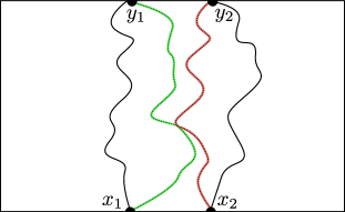
in a random potential with white-noise correlations $\overline{\eta(x,t)\eta(x^{\prime},t^{\prime})}=\delta(x-x^{\prime})\delta(t-t^{\prime})$. Then, the probability that two polymers with fixed endpoints do not cross in a given realization $\eta$ of the potential, is expressed as

$$p_{\eta}(x_{1},x_{2};y_{1},y_{2}|t)\equiv 1-\frac{Z_{\eta}(x_{2};y_{1}|t)Z_{\eta}(x_{1};y_{2}|t)}{Z_{\eta}(x_{1};y_{1}|t)Z_{\eta}(x_{2};y_{2}|t)}$$ (2)

since all paths with at least one intersection can be obtained from paths with $y_{1},y_{2}$ exchanged Karlin et al. (1959); *gessel1985binomial; *gessel1989determinants; *wiki:lgvlem (see Fig. 1). For simplicity, we will consider the random variable defined by the limit of near-coinciding endpoints

$$p_{\eta}(t)\equiv\lim_{\epsilon\to 0}\frac{p_{\eta}(-\epsilon,\epsilon;-\epsilon,\epsilon|t)}{4\epsilon^{2}}=\left.\partial_{x}\partial_{y}\ln Z_{\eta}(x;y|t)\right|_{\begin{subarray}{c}x=0\\ y=0\end{subarray}}$$ (3)

where the last equality, derived from (2), belongs to a larger set of relations between non-crossing probabilities and the single path free energy Note (1) Note (3). We now present a technique to calculate all the moments of $p_{\eta}(t)$ at arbitrary time $t$ with explicit results for the first few.

Replica trick and nested-Bethe ansatz. —

The average of products $\mathcal{Z}_{n}=\overline{Z_{\eta}(x_{1};y_{1}|t)\ldots Z_{\eta}(x_{n};y_{n}|t)}$ satisfies brunet2000probability

$$\mathcal{Z}_{n}(\mathbf{x};\mathbf{y}|t)=\langle x_{1}\ldots x_{n}|e^{-tH_{n}}|y_{1}\ldots y_{n}\rangle$$ (4)

for any integer $n$, in quantum mechanical notations, where bold symbols are shorthand for ordered sets of variables and the Lieb-Liniger Hamiltonian reads:

$$H_{n}\equiv-\sum_{i=1}^{n}\partial_{x_{i}}^{2}+2c\sum_{1\leq i<j\leq n}\delta(x_{i}-x_{j})$$ (5)

with $c=-\bar{c}<0$. To use the replica trick we introduce

$$\Theta_{n,m}(t)\equiv\lim_{\epsilon\to 0}\overline{[(2\epsilon)^{-2}Z_{\eta}^{(2)}(\epsilon)]^{m}[Z_{\eta}(0;0|t)]^{n-2m}}$$ (6)

where we set $Z^{(2)}_{\eta}(\epsilon)\equiv Z_{\eta}(\epsilon;\epsilon|t)Z_{\eta}(-\epsilon;-\epsilon|t)-Z_{\eta}(-\epsilon;\epsilon|t)Z_{\eta}(\epsilon;-\epsilon|t)$, so that $\overline{p_{\eta}(t)^{m}}=\Theta_{0,m}(t)$. The advantage of this expression is that for integers $n,m$ with $n\geq 2m$, it can be expressed in terms of (4):

$$\Theta_{n,m}(t)=\lim_{\epsilon\to 0}(2\epsilon)^{-2m}\langle{\Psi_{m}}(\epsilon)|e^{-tH_{n}}|\Psi_{m}(\epsilon)\rangle=$$

$$=\sum_{\mu}\frac{|\mathcal{D}_{m}\psi_{\mu}(\bm{0})|^{2}}{||\mu||^{2}}e^{-tE_{\mu}}$$ (7)

where $|\Psi_{m}(\epsilon)\rangle=2^{-m/2}(\otimes_{j=1}^{m}\mathinner{|{\epsilon,-\epsilon}\rangle}-\mathinner{|{-\epsilon,\epsilon}\rangle})\otimes\mathinner{|{0\ldots 0}\rangle}$ and a complete set of eigenstates $\mathinner{|{\mu}\rangle}$ of $H_{n}$ of energies $E_{\mu}$ has been inserted with $\psi_{\mu}(\mathbf{x})\equiv\mathinner{\langle\mathbf{x}|\mu\rangle}$. Here $\mathcal{D}_{m}$ is a differential operator obtained from the limit $\epsilon\to 0$ of $(2\epsilon)^{-m}\mathinner{\langle\Psi_{m}(\epsilon)|\mu\rangle}$, e.g. $\mathcal{D}_{1}=\left.2^{-1/2}(\partial_{x_{1}}-\partial_{x_{2}})\right|_{\mathbf{x}=0}$. Since $H_{n}$ is integrable by Bethe-ansatz, the eigenstates, with eigenvalues $E_{\mu}=\sum_{j=1}^{n}\mu_{j}^{2}$, take the form

$$\psi_{\mu}(\mathbf{x})=\sum_{P,Q\in\mathcal{S}_{n}}\vartheta_{Q}(\mathbf{x})A_{Q}^{P}\exp\bigl{[}i\sum_{j=1}^{n}x_{Q_{j}}\mu_{P_{j}}\bigr{]}$$ (8)

where $\{\mu_{1},\ldots,\mu_{n}\}$ is a set of rapidities, $\mathcal{S}_{n}$ the set of $n$-permutations and $\vartheta_{Q}(\mathbf{x})$ the indicator of the sector $x_{Q_{1}}\leq x_{Q_{2}}\ldots\leq x_{Q_{n}}$. However, $|\Psi_{m}(\epsilon)\rangle$ is not a symmetric state under the exchange of the coordinates, thus the quantum dynamics described by (5) does not belong to the bosonic sector. Nonetheless, it is still possible to explicitly determine the eigenstates NBAref , corresponding to different representations of the symmetric group. It is enough to choose the vectors $A_{Q}^{P}$, for all fixed permutation $P$, inside an irreducible representation of $S_{n}$. The relevant case for us is the representation corresponding to a two-rows Young diagram $\xi=(n-m,m)$, where we denote a diagram as the decreasing sequence of row lengths Fulton and Harris (1991). For instance, for $n=8$ and $m=3$ we have

$$\Yvcentermath 1(5,3)\equiv\young(13579,246)\;.$$ (9)

and the filling indicates antisymmetric wave-functions under the exchange of coordinates $\mathinner{x_{1}\leftrightarrow x_{2}},\mathinner{x_{3}\leftrightarrow x_{4}},\mathinner{x_{5}\leftrightarrow x_{6}}$, which are in the symmetry class selected by the action of $\mathcal{D}_{m=3}$. These representations can be built explicitly as the Hilbert space of an integrable spin-$1/2$ chain with $n$ sites restricted to the sector with $m$ down spins. Then the eigenstates of $H_{n}$ on a ring of length $L$ are obtained diagonalizing simultaneously the spin-model. This leads to the so-called nested-Bethe-ansatz (NBA) equations

$$\prod_{\begin{subarray}{c}b=1\\ b\neq a\end{subarray}}^{m}\frac{\lambda_{ab}-ic}{\lambda_{ab}+ic}=\prod_{j=1}^{n}\frac{\lambda_{a}-\mu_{j}-ic/2}{\lambda_{a}-\mu_{j}+ic/2}\;,$$ (10a)

$$\prod_{\begin{subarray}{c}k=1\\ k\neq j\end{subarray}}^{n}\frac{\mu_{jk}+ic}{\mu_{jk}-ic}\times\prod_{a=1}^{m}\frac{\mu_{j}-\lambda_{a}-ic/2}{\mu_{j}-\lambda_{a}+ic/2}=e^{i\mu_{j}L}$$ (10b)

where $\mu_{\alpha\beta}=\mu_{\alpha}-\mu_{\beta}$ and same for the $\lambda$’s, the auxiliary rapidities on the spin chain that impose the appropriate symmetry to the wave-function. Solutions of (10) provide the eigenstates of (5) in the appropriate symmetry class and the wave-functions are obtained setting $A_{Q}^{P}=A_{\text{\tiny bos}}^{P}\mathinner{\llangle\Psi_{Q}|\omega(P\bm{\mu})\rrangle}$ with

$$\mathinner{|{\omega(\bm{\mu})}\rrangle}=\sum_{a_{1},\ldots,a_{m}=1}^{n}\alpha(\mathbf{a}|\bm{\mu})\sigma_{-}^{a_{1}}\ldots\sigma_{-}^{a_{m}}\mathinner{|{+}\rrangle}\;.$$ (11)

Here, $(P\mu)_{j}\equiv\mu_{P_{j}}$ and $\mathinner{|{\ldots}\rrangle}$ indicates states in the auxiliary spin space, $\sigma_{-}^{a}$ is the lowering spin operator at site $a$, $a=1,\ldots,m$, acting on the reference state $\mathinner{|{+}\rrangle}=\mathinner{|{\uparrow\ldots\uparrow}\rrangle}$. The vector of states $\mathinner{|{\Psi_{Q}}\rrangle}$ is fixed by the filling of $\xi$ and performs the unitary mapping between the spin-chain representation and a particular representation of shape $(n-m,m)$, such that the exchange of two-spins is mapped into the exchange of two particles. Here $A_{\text{\tiny bos}}^{P}=\Omega_{\bm{\mu}}^{0}/\Omega_{P\bm{\mu}}$ accounts for the bosonic phase scattering with $\Omega_{\bm{\mu}}\equiv\prod_{\begin{subarray}{c}j<l\end{subarray}}f(\mu_{lj})$, $\Omega_{\bm{\mu}}^{0}=\sqrt{\Omega_{\bm{\mu}}\Omega_{-\bm{\mu}}}$ and $f(u)\equiv u/(u-ic)$, while

$$\alpha(\mathbf{a}|\bm{\mu}) =\operatorname{sym}_{\bm{\lambda}}\left[\prod_{k<l}\left(1+\frac{ic\operatorname{sgn}(a_{lk})}{\lambda_{lk}}\right)\prod_{l=1}^{m}\kappa_{a_{l}}(\lambda_{l}|\bm{\mu})\right]\;,$$

$$\kappa_{a}(u|\bm{\mu}) =\frac{ic}{u-\mu_{a}-ic/2}\prod_{b=a}^{n}\frac{u-\mu_{b}-ic/2}{u-\mu_{b}+ic/2}\;.$$

and $\operatorname{sym}_{\bm{\lambda}}[W(\bm{\lambda})]=\sum_{R}W(R\bm{\lambda})/m!$ is the symmetrization of $W(\bm{\lambda})$ over the variables $\bm{\lambda}$.

Average of $p_{\eta}(t)$. —

We now consider the case $m=1$ which selects the subspace of wave-functions $\Psi_{\bm{\mu}}(x_{1}=x_{2})=0$. Then, the wave-function in (8) remains continuous, even after the action of $\mathcal{D}_{1}$, and we can average over different orderings of the coordinates $\mathbf{x}$. Hence $\mathcal{D}_{1}\psi_{\mu}(\bm{0})=\frac{1}{n!}\sum_{P,Q}d_{1}(Q^{-1}P\bm{\mu})A_{Q}^{P}$, where $d_{m}(\bm{\mu})=(-i)^{m}\mathcal{D}_{m}e^{i\bm{\mu}\cdot\mathbf{x}}|_{\mathbf{x}=0}$. We then obtain Note4

$$\frac{1}{n!}\sum_{Q}d_{1}(Q^{-1}\bm{\mu})\mathinner{|{\Psi_{Q}}\rrangle}=\sqrt{Z}{\sum_{a=1}^{n}}(\mu_{a}-\hat{\mu})\sigma_{-}^{a}\mathinner{|{+}\rrangle}$$ (12)

with $Z=[(n-1)n!]^{-1}$ ensuring normalization and $\hat{\mu}=\sum_{b}\mu_{b}/n$. It leads to $|\mathcal{D}_{1}\psi_{\mu}(\bm{0})|^{2}=n(n-2)!|\Omega_{\bm{\mu}}|^{2}|\mathcal{F}(\lambda,\bm{\mu})|^{2}$, where $\mathcal{F}(\lambda,\bm{\mu})=\operatorname{sym}_{\bm{\mu}}\left[\Omega_{\bm{\mu}}^{-1}\sum_{a}(\mu_{a}-\hat{\mu})\kappa_{a}(\lambda|\bm{\mu})\right]$ and we note $\lambda_{a=1}=\lambda$. The sum over all solutions of (10) must then be performed according to (Replica trick and nested-Bethe ansatz. —), a formidable task in general. However, (10b) simplifies dramatically when $L\to\infty$. For $\bar{c}>0$, the $n$ rapidities $\mu_{1},\ldots,\mu_{n}$, are organized in $n_{s}$ bound states, each composed by $m_{j}\geq 1$ particles, with $\sum_{j=1}^{n_{s}}m_{j}=n$. The rapidities inside a bound state follow a regular pattern in the complex plane $\mu^{j,a}=k_{j}+\frac{i\bar{c}}{2}(m_{j}+1-2a)+i\delta^{j,a}$, named string. Here $a=1,\ldots,m_{j}$ labels the rapidities inside the string and $\delta^{j,a}$ are exponentially small for large $L$. A study of (10) reveals that, at variance with the bosonic case, not all string configurations are actually allowed, consistently with the symmetry of the wave-function Note (1). For those allowed, using Calabrese and Caux (2007); Pozsgay et al. (2012), we obtain their norm Note5 as:

$$\frac{||\psi_{\mu}||^{2}}{(\Omega_{\bm{\mu}}^{0})^{2}} =\frac{(L\bar{c})^{n_{s}}\prod_{j}m_{j}^{2}}{\bar{c}^{n}\Phi(\mathbf{k},\mathbf{m})}{\sum_{l=1}^{n}}\frac{4c^{2}}{c^{2}+4(\mu_{l}-\lambda)^{2}}\;,$$ (13)

$$\Phi(\mathbf{k},\mathbf{m}) =\prod_{1\leq j<j^{\prime}\leq n_{s}}\frac{(k_{j}-k_{j^{\prime}})^{2}+c^{2}(m_{j}-m_{j^{\prime}})^{2}/4}{(k_{j}-k_{j^{\prime}})^{2}+c^{2}(m_{j}+m_{j^{\prime}})^{2}/4}\;.$$ (14)

For each configuration of rapidities following the string ansatz, a multiplet of eigenstates is given by the set $\{\lambda^{(1)},\ldots,\lambda^{(n-1)}\}$ of solutions of (10a), i.e. $Q(\lambda)\equiv P_{+}(\lambda)/P_{-}(\lambda)=1$, where $P_{\pm}(\lambda)=\prod_{i}(\lambda-\mu_{i}\pm ic/2)$. These values cannot be determined analytically for general $n$, however the sum over them can be performed using residue theorem

$$\sum_{i}w(\lambda^{(i)})=\oint_{\mathcal{C}}\frac{dz}{2\pi i}w(z)\frac{Q^{\prime}(z)}{Q(z)-1}$$

where $w(z)$ is any analytic function inside the contour $\mathcal{C}$, which encircles all the solutions $\lambda^{(i)}$ and no other singularity of the integrand. Equivalently, the integral can be computed taking the poles outside the contour, which in the case $w(z)=\frac{|\mathcal{F}(\lambda^{(i)},\bm{\mu})|^{2}}{||\psi_{\mu}||^{2}}$, are given by $z_{k}=\mu_{k}-ic/2$ Note5 . The sum can then be performed analytically. Moreover, for $L\to\infty$, string momenta become free and we can replace $\sum_{k_{j}}\to m_{j}L\int\frac{dk_{j}}{2\pi}$, which leads to

$$\Theta_{n,1}(t)=\sum_{n_{s}=1}^{n}\frac{n!\bar{c}^{n}}{n_{s}!(2\pi\bar{c})^{n_{s}}}\sum_{(m_{1},..m_{n_{s}})_{n}}$$ (15)

$$\prod_{j=1}^{n_{s}}\int_{-\infty}^{+\infty}\frac{dk_{j}e^{-A_{2}t}}{m_{j}}\Phi(\mathbf{k},\mathbf{m})\Lambda_{n,1}(\mathbf{k},\mathbf{m})$$

with $\Lambda_{n,1}=(n(n-1))^{-1}h_{2}$. Here, $(m_{1},\ldots,m_{n_{s}})_{n}$, indicates sum over all integers $m\geq 1$ whose sum equals $n$ and we defined $h_{p}=\sum_{j<l}(\mu_{j}-\mu_{l})^{p}-(i\bar{c})^{p}(j-l)^{p}$. The rapidities $\mu_{j}$ are written as a function of string sizes and momenta according to the string ansatz, so that $\Lambda_{n,1}$ vanishes on the $n$-strings. The conserved charges of the Lieb-Liniger model have been introduced as $A_{p}=\sum_{j=1}^{n}\mu_{j}^{p}$, $A_{2}$ being the energy. A crucial property of (15) is that by replacing $\Lambda_{n,1}\to\Lambda_{n,0}\equiv 1$, one recovers the formula for $\mathcal{Z}_{n}(t)\equiv\mathcal{Z}_{n}(\mathbf{x}=\bm{0};\bm{0}|t)=\Theta_{n,0}(t)$ as given in Calabrese et al. (2010). Therefore, rewriting $\Lambda_{n,1}$ in terms of the conserved charges and using the statistical tilt symmetry (STS) (see e.g. Appendix of flat ), we obtain

$$\Theta_{n,1}(t)=\frac{1}{n-1}\left[\frac{n(n^{2}-1)\bar{c}^{2}}{12}-\partial_{t}-\frac{1}{2t}\right]\mathcal{Z}_{n}(t)\;.$$ (16)

This expression is exact for $n\geq 2$ and allows the analytical continuation $n\to 0$. In particular, we obtain

$$\overline{p_{\eta}(t)}=\lim_{n\to 0}\Theta_{n,1}(t)=\frac{1}{2t}\;.$$ (17)

This is in fact the exact result for $p_{\eta}(t)$ without disorder, i.e. $\eta(x,t)=0$. This remarkable conclusion can also be obtained by averaging (3) and recalling that the dependence of the average free energy of a path with respect to its endpoints is entirely fixed by the STS, namely $\overline{\ln Z_{\eta}(x;y|t)}=h(t)-(x-y)^{2}/(4t)$, where

$$h(t)=\overline{\ln Z_{\eta}(0;0|t)}$$ (18)

is our averaged free energy (and average KPZ height).

Alternative derivation. —

A different approach was recently proposed in Borodin and Corwin (2014) (remark 5.25) where non-intersecting paths were also studied. There, it was proposed a multicontour-integral formula associated to a partition of $n$. We identify the partition with a Young-diagram and for the two-row case of our interest, it can be put in the form

$$\Theta_{n,m}(t)=\frac{1}{2^{m}}\int\frac{dz_{1}}{2\pi}\cdots\int\frac{dz_{n}}{2\pi}e^{-t\sum_{k=1}^{n}z_{k}^{2}}\\ \times\left(\prod_{1\leq k<j\leq n}f\bigl{(}z_{kj}\bigr{)}\right)\left(\prod_{q=1}^{m}h(z_{2q-1,2q})\right)\;.$$ (19)

where $z_{kj}=z_{k}-z_{j}$, $h(u)=u(u-ic)$ and the integration contours are parallel to the real axis with an imaginary part $C_{j}$ for $z_{j}$ satisfying $C_{j+1}>C_{j}+\bar{c}$. Shifting back all the contours to the real axis, we encounter many poles whose residues reduce to integrals with a smaller number of integration variables. This expansion can then be organized to reproduce the one based on strings in (15), with $\Lambda_{n,1}$ replaced by Note (1)

$$\Lambda_{n,m}(\mathbf{k},\mathbf{m})=\frac{1}{2^{m}}\operatorname{sym}_{\bm{\mu}}\left[\frac{\prod_{q=1}^{m}h(\mu_{2q-1,2q})}{\prod_{1\leq j<k\leq n}f(\mu_{kj})}\right]$$ (20)

and again the $\bm{\mu}$ given by the string ansatz. Interestingly, $\Lambda_{n,m}$ is always a polynomial in the $\mu$’s of degree $2m$ as can be seen considering the residue at coinciding points. Moreover, Eq. (20) agrees with the result obtained from the NBA for $m=1$, which gives a completely independent check to the proposition in (19). For $m>1$, the calculation from NBA becomes more involved but we will continue by assuming that (20) retains its validity.

Figure 2: (Color online) The first (a) and second moment (b) of $p_{\eta}$ in the continuum limit are shown vs $t$ for several value of $\beta$. Numerical simulations with at least $2\times 10^{5}$ realizations and time up to $\hat{t}=8192$. The value of $p_{\eta}$ introduced in (3) is obtained by $p_{\eta}(t)=\hat{p}/(16\beta^{4})$, with $\hat{p}$ the probability on the lattice and the time is scaled to $t$ by $\hat{t}=t/(2\beta^{4})$. Dashed red line: analytical predictions, (17) and (23). In (b), the small $t$ expansion $\overline{p_{\eta}^{2}}\simeq 4t^{-2}$ is shown with a dashed blue line. Inset in (b): plot of $\overline{\hat{p}^{2}}\,\hat{t}/\beta^{4}\simeq\beta^{-4}c_{2}(\beta)$ vs $\beta$ and extrapolation at small $\beta=0$ from the best fit with a quadratic function in $\beta$ at fixed $t=10^{3}$. It shows a finite limit consistent with our prediction $\simeq 32/3=10.6(7)$ (blue circle).

Higher moments of $p_{\eta}(t)$. —

We now focus on $m=2$. Upon symmetrization in (20) one obtains

$$\Lambda_{n,2}(\bm{\mu})=\frac{h_{2}^{2}-(n-1)h_{4}-n(n-1)^{2}\bar{c}^{2}h_{2}}{n(n-1)(n-2)(n-3)}\;.$$ (21)

After tedious calculations, it can be rewritten in terms of the conserved charges $\Lambda_{n,2}(\{A_{p}\})$ Note (1). In contrast with the $m=1$ case, higher charges, up to $p=4$, are involved. It is therefore useful to formally generalize the partition function to $\mathcal{Z}_{n}^{\bm{\beta}}(t)$ which is obtained from the expression of $\mathcal{Z}_{n}(t)$ replacing the imaginary time evolution $e^{-A_{2}t}$ with the more general $e^{-A_{2}t+\sum_{p\geq 1}\beta_{p}A_{p}}$. This is the partition function of a Generalized Gibbs ensemble (GGE) Fioretto and Mussardo (2010), which we show can be related to a Fredholm determinant Note (1). Here, we use it as a generating function: $\Theta_{n,2}(t)=\Lambda_{n,2}(\{\partial_{p}\})\mathcal{Z}_{n}^{\bm{\beta}}(t)$, formally replacing $A_{p}\to\partial_{p}\equiv\partial_{\beta_{p}}$ and setting $\beta_{p}\to 0$ at the end. Deriving extended STS identities from the invariance $\mu_{j}\to\mu_{j}+k$ in $\mathcal{Z}_{n}^{\bm{\beta}}(t)$, for arbitrary $k$, we are able to re-express it only from the energy $A_{2}$, leading to

$$\overline{p_{\eta}(t)^{2}}=-\left(\frac{1}{t}\partial_{t}+\frac{1}{2}\partial_{t}^{2}\right)h(t)\;.$$ (22)

Hence the second moment is determined at all times from the average free energy $h(t)$ (18). We did not find a direct derivation of this remarkable result, and it may be a consequence of integrability. At large time $h(t)\simeq-\frac{\bar{c}^{2}t}{12}+\overline{\chi_{2}}(\bar{c}^{2}t)^{1/3}$ Calabrese et al. (2010); dotsenko ; spohnKPZEdge ; corwinDP , so that

$$\overline{p_{\eta}(t)^{2}}\simeq\frac{\bar{c}^{2}}{12t}-\frac{2\overline{\chi_{2}}\bar{c}^{2/3}}{9t^{5/3}}$$ (23)

with $\overline{\chi_{2}}=-1.77(1)$ the mean of the Tracy-Widom GUE distribution TracyMathematical Tables and Other Aids to Computation and Widom (1994). Repeating this procedure for $m=3$ we can again use $\mathcal{Z}_{n}^{\bm{\beta}}(t)$. Now higher charges are involved and the result is expressed as derivatives of a Fredholm determinant Note (1). It simplifies at large time leading to:

$$\overline{p_{\eta}(t)^{3}}\simeq\frac{\bar{c}^{4}}{15t}-\frac{2\overline{\chi_{2}}\bar{c}^{8/3}}{9t^{5/3}}$$ (24)

It is natural to conjecture the leading decay $\overline{p_{\eta}(t)^{m}}\simeq\gamma_{m}\bar{c}^{2(m-1)}/t$ for any integer $m>1$. However, the knowledge of moments at long-times is not sufficient to reconstruct the full distribution of $p$: in view of Doumerc , we further surmise that $p_{\eta}(t)$ tends to zero (sub) exponentially at large $t$ for all but a small fraction $\sim 1/(\bar{c}^{2}t)$ of environments where typically $p_{\eta}(t)\sim\bar{c}^{2}$. This is consistent with the conjecture Note (1) $\overline{\ln p_{\eta}(t)}\sim-a(\bar{c}^{2}t)^{1/3}$ where $a=\overline{\chi_{2}}-\overline{\chi^{\prime}_{2}}$ is the average gap between the first ($\chi_{2}$) and second ($\chi^{\prime}_{2}$) GUE (scaled) largest eigenvalues, with $a\approx 1.9043$ TWNote (note that $a\approx 1.49134$ for the hard wall problem Gueudre ).

Comparison with numerics —

To check our results, we study a discrete directed polymer on a square lattice Calabrese et al. (2010), defined according to the recursion (with integer time $\hat{t}$ running along the diagonal)

$$Z_{\hat{x},\hat{t}+1}=(Z_{\hat{x}-\frac{1}{2},t}+Z_{\hat{x}+\frac{1}{2},\hat{t}})e^{-\beta V_{\hat{x},\hat{t}+1}}$$ (25)

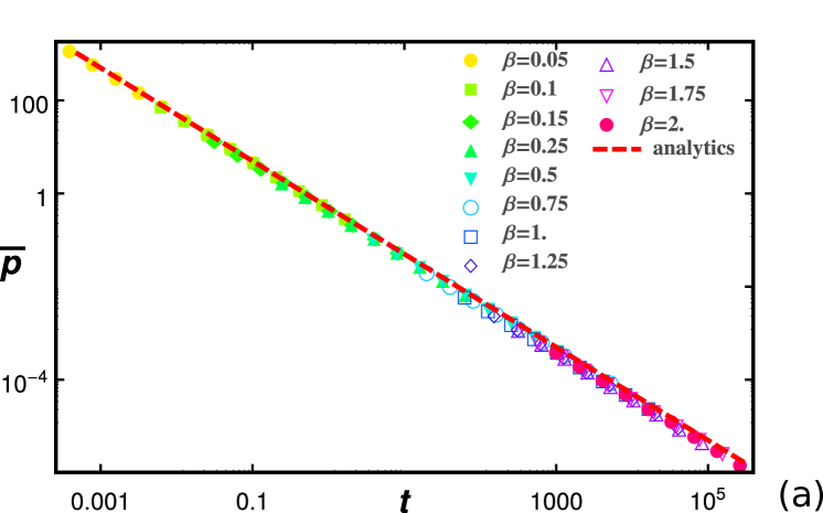
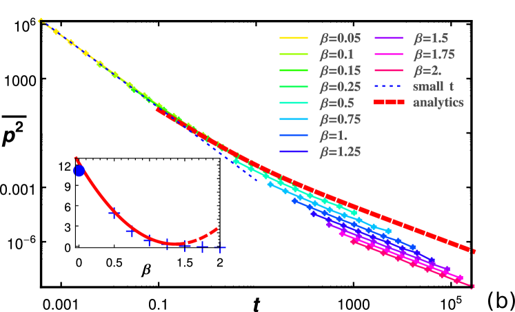
with $V_{\hat{x},\hat{t}}$ sampled from the standard normal distribution. In the high temperature limit $\beta\ll 1$, it maps into the continuous DP (1) at $\bar{c}=1$ with $x=4\hat{x}\beta^{2}$ and $t=2\hat{t}\beta^{4}$ Calabrese et al. (2010). We consider two polymers with initial conditions $Z_{\hat{x},\hat{t}=1}^{\pm}=\delta_{\hat{x},\pm 1/2}$ and ending at time $\hat{t}$ at $\hat{x}=\pm 1/2$. For each realization of the $V_{\hat{x},\hat{t}}$, the non-crossing probability $\hat{p}$ on the lattice is efficiently computed using the image method Karlin et al. (1959); *gessel1985binomial; *gessel1989determinants; *wiki:lgvlem. Comparing with (3), we deduce $\hat{p}\simeq 16p\beta^{4}$, for $\beta\to 0$, due to the rescaling of the factor $\epsilon=4\beta^{2}$. The numerical results and the analytical predictions (17, 23) are shown in Fig. 2. For the first moment $\overline{p_{\eta}(t)}$ the agreement is excellent even at finite temperature, presumably due to robustness of (17) at any time. The numerical check of (23) is more delicate: indeed, the large-time behavior of the second moment depends strongly on temperature and approaches our prediction only for $\beta\ll 1$, see Fig. 2 (right). However, the leading decay is found consistent with $t^{-1}$ down to zero temperature, where the polymer paths do not fluctuate thermally and for any $m>0$: $\overline{\hat{p}^{m}}=\overline{\hat{p}}$. In order to interpolate between zero and high temperatures, we conjecture the large time behavior of the moments on the lattice: $\overline{\hat{p}^{m}}\simeq c_{m}(\beta)/\hat{t}$, with $c_{m}(\beta)\simeq\gamma_{m}2^{4m-1}\beta^{4(m-1)}$ at high temperatures and $c_{m}(\beta\to\infty)=c_{\infty}$ is a constant that we expect to be non-universal Note (1). This agrees with the intuitive picture of the zero temperature deterministic path, weakly perturbed by thermal fluctuations. Checking the sub-leading terms in (23) would require much more intensive numerics.

Conclusions. —

We presented a general formalism to calculate the statistics of $N$ mutually avoiding directed polymers in a random potential, with explicit results for $N=2$. Multi-polymer observables are reduced to a compact form in terms of conserved quantities of the Lieb-Liniger Hamiltonian and expressed at all times by derivatives of a Fredholm determinant, i.e. the GGE partition function. As a simplest example we obtained the lowest moments of non-crossing probabilities, with an exact relation between the variance and the free-energy, a non trivial scaling $t^{-5/3}$ for the sub-leading part and a prediction of leading behavior for all moments. The full distribution of the non-crossing probability is under current investigation. Going beyond the infinite hard-core repulsion remains for the moment elusive, but we are confident that further developments of the present method and full exploitation of its integrable structure, will allow further progress in the elusive interplay between disorder and interactions.

Acknowledgements. —

We thank A. Borodin, I. Corwin and A. Rosso for fruitful discussions. This work is supported by “Investissements d’Avenir” LabEx PALM (ANR-10-LABX-0039-PALM) and by PSL grant ANR-10-IDEX-0001-02-PSL.

Supplementary Material for EPAPS
The crossing probability for directed polymers in random media.

Here we give additional details about

• crossing probabilities of paths;

• the construction of the representations of the symmetric group;

• the explicit derivation of the $m=1$ from the nested-Bethe ansatz;

• the generalization to arbitrary initial conditions from the expansion of the multi-contour integral formula;

• the derivation of a Fredholm determinant formula for the generalized generating function.

• the extension of the STS symmetry and the calculation of the $m=1,2,3$ moments;

We will conventionally use $\xi$ (and $\chi$) to indicate Young diagrams of size $n$, with $\xi_{i}$ ($\xi^{i}$) the size of rows (columns) from top to bottom (left to right). We write each diagram as the sequence of decreasing row sizes $\xi\equiv(\xi_{1}\xi_{2}\ldots)$, $\xi_{1}\geq\xi_{2}..\geq\xi_{n_{R}(\xi)}$. Equivalently, one can write it as a sequence of decreasing column sizes. There is a correspondence (bijective in each case) between these two sets of sequences, and the partitions of the integer $n$, as $\sum_{\alpha=1}^{n_{R}(\xi)}\xi_{\alpha}=\sum_{\alpha=1}^{n_{C}(\xi)}\xi^{\alpha}=n$, with $\xi_{\alpha}\geq\xi_{\alpha^{\prime}}$ when $\alpha<\alpha^{\prime}$ and the same for $\xi^{\alpha},\xi^{\alpha^{\prime}}$. A standard tableau ${\bar{\xi}}$ is obtained from the diagram $\xi$ by filling the boxes with the integers $1,\ldots,n$, with the condition that they grow from left/right and top/bottom along each row and column.

I Crossing probabilities and the free energy

Here we show relations, valid in any given disorder realization, between non-crossing probabilities of several paths and the free energy of a single path. Consider $N$ directed paths $x_{i}(\tau)$ in the continuum, with endpoints $x_{i}(0)=y_{i}$, $x_{i}(t)=y_{i}$ and $x_{1}<x_{2}<..x_{N}$, $y_{1}<y_{2}<..y_{N}$. We know from the Karlin-McGregor formula and generalizations Karlin et al. (1959); *gessel1985binomial; *gessel1989determinants; *wiki:lgvlem that the probability that these paths do not cross can be expressed as a determinant:

$$p_{\eta}^{(N)}(x_{1},\ldots,x_{N};y_{1},\ldots,y_{N}|t)=\prod_{i=1}^{N}\frac{1}{Z_{\eta}(x_{i};y_{i}|t)}{\rm det}[Z_{\eta}(x_{i};y_{j}|t)]_{N\times N}$$ (S1)

Consider first $N=2$ which is the main focus of this work. Bringing two endpoints close together, i.e. $y_{1,2}=y\mp\epsilon/2$ and dividing by $\epsilon$, equivalently applying the operator $O_{2}(y)=\frac{1}{2}(\partial_{y_{2}}-\partial_{y_{1}})|_{y_{2}=y_{1}=y}$, or equivalently for $x_{12}$ we obtain:

$$p^{(2)}_{\eta}(x_{1},x_{2};y|t)=\partial_{y}(\ln Z_{\eta}(x_{2};y|t)-\ln Z_{\eta}(x_{1};y|t))$$ (S2)

$$p^{(2)}_{\eta}(x;y_{1},y_{2}|t)=\partial_{x}(\ln Z_{\eta}(x;y_{2}|t)-\ln Z_{\eta}(x;y_{1}|t))$$ (S3)

Bringing points together on both ends we obtain the non-crossing probability for 2 paths both from $y$ to $x$:

$$p^{(2)}_{\eta}(x;y|t):=O_{2}(x)O_{2}(y)p^{(2)}_{\eta}(x_{1},x_{2};y_{1},y_{2}|t)=\partial_{x}\partial_{y}\ln Z_{V}(x;y|t)$$ (S4)

In particular this leads to Eq. (3) for the quantity defined in the text $p_{\eta}(t):=p^{(2)}_{\eta}(0;0|t)$. Note that the STS symmetry also implies

$$\overline{p^{(2)}_{\eta}(x_{1},x_{2};y|t)}=\frac{x_{2}-x_{1}}{2t}\quad,\quad p^{(2)}_{\eta}(x;y_{1},y_{2}|t)=\frac{y_{2}-y_{1}}{2t}\quad,\quad\overline{p^{(2)}_{\eta}(x;y|t)}=\frac{1}{2t}$$ (S5)

in addition to the result mentioned in the text. Note that these STS results are exact also for a model with a more general noise, provided it has the STS symmetry, e.g. $\overline{\eta(x,t)\eta(x^{\prime},t^{\prime})}=\delta(t-t^{\prime})R(x-x^{\prime})$.

Similar relations, although more involved, exist for more than 2 paths, $N>2$. For instance the non-crossing probabilities with one endpoint coinciding, defined as $p_{\eta}^{(N)}(x;y_{1},..y_{N},t)=O_{N}(x)p_{\eta}^{(N)}(x_{1},..x_{N};y_{1},..y_{N},t)$ where now $O(x)=\frac{1}{N!}\prod_{1\leq i<j\leq N}(\partial_{j}-\partial_{i})|_{x_{a}=x}$, admits a simple expression as a determinant:

$$p_{\eta}^{(N)}(x;y_{1},..y_{N}|t)=det[\frac{\partial_{x}^{i-1}Z_{\eta}(x,y_{j})}{Z_{\eta}(x,y_{j})}]_{N\times N}$$ (S6)

the first row of the matrix being the vector $(1,..,1)$. Such derivatives can then be re-expressed in terms of derivatives of the free energy. Taking the second endpoint coinciding by applying $O_{N}(y)$ leads to, e.g. for $N=3$:

$$p^{(3)}_{\eta}(x;y|t)=p^{(2)}_{\eta}(x;y|t)\partial_{x}\partial_{y}p^{(2)}_{\eta}(x;y|t)-\partial_{x}p^{(2)}_{\eta}(x;y|t)\partial_{y}p^{(2)}_{\eta}(x;y|t)+2p^{(2)}_{\eta}(x;y|t)^{3}$$ (S7)

where we recall $p^{(2)}_{\eta}(x;y|t)=\partial_{x}\partial_{y}\ln Z_{\eta}(x;y|t)$, and to more complicated relations for higher $N$.

Dependence in elastic coefficient and a conjecture for discrete model:

If, in the continuum model described by Eq. (1) the elasticity term $\int_{0}^{t}d\tau\frac{1}{4}(\frac{dx}{d\tau})^{2}$ is replaced by $\int_{0}^{t}d\tau\frac{\kappa}{4}(\frac{dx}{d\tau})^{2}$ in Eq. (1) to study the effect of elasticity $\kappa$, the above result is trivially changed into $\overline{p^{(2)}_{\eta}(x;y|t)}=\frac{\kappa}{2{\sf T}t}$.

Let us now consider a discrete DP model on a lattice, e.g. as the one defined in the text. This model does not satisfy exact STS anymore. However it can usually be described by an effective elastic constant $\kappa_{eff}(T)$ defined from the curvature around a minimum of the average free energy with respect to one end-point position. It may, in general depend on the temperature (defined for the lattice model). Hence we can conjecture that the large time limit of the observable $\overline{\hat{p}}$ defined in the text will be $\overline{\hat{p}}\sim\frac{4\kappa_{eff}(T)}{\hat{t}}$ (such that for the discrete model defined in the text $\kappa_{eff}(T\to\infty)=1$).

II Representations of the symmetric group

The eigenfunctions of $H_{n}$ in Eq.(5) are contained in $\mathcal{L}^{2}([0,L]^{n})$. Because of the integrability of the model, the eigenfunctions can be written as linear combination of plane-waves in each sector $x_{Q_{1}}\leq\ldots\leq x_{Q_{n}}$ as in (8). Since $H_{n}$ is symmetric under the exchange of coordinates, they can be classified according to the representations of the symmetric group. For a fixed $P$, the vector of components $A_{Q}^{P}$ belongs to a vector space $V$ of dimension $n!$. In this space it is naturally defined a representation of the symmetric group $\mathcal{S}_{n}$, called the regular representation, where the action of a permutation $T\in\mathcal{S}_{n}$ is simply the left multiplication and the matrix representation is $\mathcal{L}(T)_{Q,Q^{\prime}}=\delta_{T^{-1}Q,Q^{\prime}}$. In a similar way, it is defined the dual representation based on the right multiplication $\mathcal{R}(T)_{Q,Q^{\prime}}=\delta_{QT^{-1},Q^{\prime}}$, associated with the exchange of two coordinates (see below). Note that $\mathcal{L}(T_{1})\mathcal{L}(T_{2})=\mathcal{L}(T_{1}T_{2})$ while $\mathcal{R}(T_{1})\mathcal{R}(T_{2})=\mathcal{R}(T_{2}T_{1})$; moreover $\mathcal{L}(T_{1})\mathcal{R}(T_{2})=\mathcal{R}(T_{2})\mathcal{L}(T_{1})$.

Moreover, the requirements for (8) to be an eigenstates imposes that Yang (1967)

$$A_{Q}^{\sigma_{i}P}=\sum_{Q^{\prime}\in\mathcal{S}_{n}}[Y^{\sigma_{i}}_{P_{i}P_{i+1}}]_{Q,Q^{\prime}}A_{Q^{\prime}}^{P}$$ (S8)

where $\sigma_{i}$ is the transposition permutation exchanging $i,i+1$ and $Y^{\sigma_{i}}_{ab}=f(\mu_{ba})\mathcal{L}(\sigma_{i})+(f(\mu_{ba})-1)\mathcal{L}(\mathbf{1})$ with $\mathbf{1}$ the identical permutation. This ensures that all the vectors $A_{Q}^{P}$ for different $P$ can be chosen inside an irreducible representation of $\mathcal{S}_{n}$, which are in one-to-one correspondence with Young diagrams Fulton and Harris (1991). It is useful to summarize the construction. Given a standard tableau ${\bar{\xi}}$, we associate two subgroups of $\mathcal{S}_{n}$: $\mathcal{A}({\bar{\xi}})$ and $\mathcal{B}({\bar{\xi}})$ defined respectively as the two subgroups that preserve respectively rows and columns, i.e. $\mathcal{A}({\bar{\xi}})$ are all permutations within rows, and $\mathcal{B}({\bar{\xi}})$ within columns. Two elements of the group algebra of $\mathcal{S}_{n}$ are then defined as

$$a({\bar{\xi}})=\sum_{P\in\mathcal{A}({\bar{\xi}})}P\;,\quad b({\bar{\xi}})=\sum_{P\in\mathcal{B}({\bar{\xi}})}(-1)^{\sigma_{P}}P$$ (S9)

from which we define the Young symmetrizer

$$c({\bar{\xi}})=a({\bar{\xi}})b({\bar{\xi}})=\sum_{P\in\mathcal{S}_{n}}c_{P}P\;.$$ (S10)

The coefficients $c_{P}$ are integer numbers obtained from (S9). The Young symmetrizer projects onto $V_{\bar{\xi}}=\mathcal{R}(c({\bar{\xi}}))V$, an irreducible representation under the left-action $\mathcal{L}(\mathcal{S}_{n})V_{\bar{\xi}}$, where $\mathcal{R}$ has been extended on the group algebra by linearity e.g. $\mathcal{R}(a({\bar{\xi}}))=\sum_{P\in\mathcal{A}({\bar{\xi}})}\mathcal{R}(P)$. The wave-functions built using the vectors $A_{Q}^{P}$ in $V_{\bar{\xi}}$ are anti-symmetric on the variables inside each column. Indeed for any permutation $T\in\mathcal{S}_{n}$:

$$\psi_{\mu}(T\mathbf{x})=\sum_{P,Q\in\mathcal{S}_{n}}\vartheta_{Q}(\mathbf{x})A_{QT^{-1}}^{P}\exp\bigl{[}i\sum_{i}x_{Q_{i}}\mu_{P_{i}}\bigr{]}$$ (S11)

using that $(QT{\bf x})_{j}=(T{\bf x})_{Q_{j}}=x_{T_{Q_{j}}}$ and performing the relabeling $Q\to QT^{-1}$. Now, for $T\in\mathcal{B}({\bar{\xi}})$ one finds that:

$$\psi_{\mu}(T\mathbf{x})=(-1)^{\sigma_{T}}\sum_{P,Q\in\mathcal{S}_{n}}\vartheta_{Q}(\mathbf{x})A_{Q}^{P}\exp\bigl{[}i\sum_{i}x_{Q_{i}}\mu_{P_{i}}\bigr{]}$$ (S12)

In the last equality, we used that for any vector $v\in V_{\bar{\xi}}$, $v=\mathcal{R}(b({\bar{\xi}}))v^{\prime}$ for some $v^{\prime}\in V$, and therefore $\mathcal{R}(T)v=\mathcal{R}(b({\bar{\xi}})T)v^{\prime}=\sum_{P\in\mathcal{B}({\bar{\xi}})}(-1)^{\sigma_{P}}\mathcal{R}(PT)v^{\prime}=(-1)^{\sigma_{T}}\mathcal{R}(b({\bar{\xi}}))v^{\prime}=(-1)^{\sigma_{T}}v$.

An alternative path is to build the irreducible representations of $S_{n}$ using the Hilbert space $G$ of $n$ spin $1/2$. The action $\mathcal{G}(T)$ of a permutation $T$ is defined as the permutation of the spins

$$\mathcal{G}(T)\mathinner{|{i_{1}\ldots i_{n}}\rrangle}=\mathinner{|{i_{T_{1}}\ldots i_{T_{n}}}\rrangle}$$ (S13)

where $i_{k}\in\{\uparrow,\downarrow\}$, the two eigenstates of the $k$-th spin along the $z$-direction. The sub-space $G_{\xi}$ of highest weights, i.e. annihilated by $S^{+}=\sum_{k}s^{+}_{k}$, with fixed total magnetization $S^{z}=\sum_{k}s^{z}_{k}=(n-2m)/2$, defines the irreducible representation corresponding to the two-rows diagram $\xi=(n-m,m)$. This procedure can be extended to the general case and allows deriving the equations for the rapidities $\bm{\mu}$, together with a hierarchy of auxiliary rapidities for each row of $\xi$, called nested-Bethe-Ansatz equations Sutherland (1968). For the two-rows diagrams, we get (10) in the text. Although these equations only depend on the diagram $\xi$, wave-functions depend on the tableau ${\bar{\xi}}$. For instance, for $n=3$ and $m=1$, we have two possible tableaux

$$\Yvcentermath 1(2,1)_{1}=\young(12,3)\;,\qquad(2,1)_{2}=\young(13,2)\;.$$ (S14)

All the possible standard tableaux correspond to different copies of a given irreducible representation inside the regular one and therefore to different multiplets of wave-functions. For a general two-row diagram the dimension of the irreducible representation is

$$d_{\xi}=d_{(n-m,m)}={n\choose{m}}\left(\frac{n-2m+1}{n-m+1}\right)$$ (S15)

and its multiplicity inside the regular representation is also equal to $d_{\xi}$ Fulton and Harris (1991). The spin-representation can be mapped into each of these copies by a linear mapping $\Psi:V\to G$, with components $\Psi(v)=\sum_{Q}v_{Q}\mathinner{|{\Psi_{Q}}\rrangle}$, for any vector $v\in V$ of components $v_{Q}$. A complete characterization of this mapping is obtained requiring that, for each choice ${\bar{\xi}}$ for the same $\xi$,

• $\Psi(V_{\bar{\xi}})\equiv G_{\xi}$, unitarily so that, for any $w\in V_{{\bar{\xi}}}$

  $$||w||^{2}\equiv\sum_{Q}|w_{Q}|^{2}=||\Psi(w)||^{2}$$ (S16)

• for any $w\in V_{{\bar{\xi}}}$:

  $$\Psi(\mathcal{L}(T)w)=\mathcal{G}(T)\Psi(w)$$ (S17)

• we fix the action of $\Psi$ on the space orthogonal to $V_{{\bar{\xi}}}$ by $\sum_{Q}\mathinner{|{\Psi_{Q}}\rrangle}\mathinner{\llangle{\Psi_{Q}}|}=\Pi_{\xi}$, with $\Pi_{\xi}$ the projector of $G$ onto $G_{\xi}$.

With these definitions, we take

$$A_{Q}^{P}=A_{\text{\tiny bos}}^{P}\mathinner{\llangle\Psi_{Q}|\omega(P\bm{\mu})\rrangle}\;.$$ (S18)

In practice, the explicit form of $\Psi$ is not needed, since the differential operator $\mathcal{D}_{m}$ gives a non-vanishing result only for one Young tableau ${\bar{\xi}}_{0}$, corresponding to the filling described in (9). In order to show this, we now give the explicit derivation of Eq.(12) in the main text. The vector of components $v_{Q}^{(m)}=d_{m}(Q^{-1}\bm{\mu})$ belongs to $V_{{\bar{\xi}}_{0}}$ and we only need the image $\mathinner{|{m}\rrangle}\equiv\Psi(v^{(m)})=\sum_{Q}d_{m}(Q^{-1}\bm{\mu})\mathinner{|{\Psi_{Q}}\rrangle}$ of this vector in the spin representation $G_{{\bar{\xi}}_{0}}$. To determine it, we expand it as

$$\mathinner{|{m}\rrangle}=\sum_{a_{1},\ldots,a_{m}=1}^{n}q_{a_{1},\ldots,a_{m}}(\bm{\mu})\sigma_{-}^{a_{1}}\ldots\sigma_{-}^{a_{m}}\mathinner{|{+}\rrangle}$$ (S19)

where $q_{a_{1},\ldots,a_{m}}(\bm{\mu})$ is a symmetric tensor obtained as a linear combination of the $v_{Q}^{(m)}$. Its components are therefore homogeneous polynomials in the $\bm{\mu}$ of degree $m$Because of (S17), under the mapping $\Psi$, a permutation of the rapidities $\bm{\mu}$ corresponds to a permutation of spins, we deduce the expansion

$$q_{a_{1},\ldots,a_{m}}(\bm{\mu})=\sum_{k=0}^{m}q_{k}^{1}(\bm{\mu})q_{m-k}^{2}(\mu_{a_{1}},\ldots,\mu_{a_{m}})$$ (S20)

where $q_{k}^{1,2}$ are symmetric polynomials of degree $k$. Moreover, from $S^{+}\mathinner{|{m}\rrangle}=0$, we have

$$\sum_{\begin{subarray}{c}a=1\\ a\neq a_{2},\ldots,a_{m}\end{subarray}}^{n}q_{aa_{2}\ldots a_{m}}=0\;.$$ (S21)

These conditions are sufficient to determine the state $\mathinner{|{m}\rrangle}$ and in particular for $m=1$, they lead to

$$q_{a}=\sqrt{Z}(\mu_{a}-\hat{\mu})\;,$$ (S22)

where $\hat{\mu}=\frac{1}{n}\sum_{a=1}^{n}\mu_{a}$ and, since $\Psi$ satisfies (S16), $Z$ can be fixed equating $\sum_{Q}|v_{Q}^{(m)}|^{2}\equiv||v_{Q}^{(m)}||^{2}=\mathinner{\llangle m|m\rrangle}$, recovering (12).

III Nested Bethe ansatz approach

III.1 Norm of a state: general form

The expression of the norm for a given set of $\bm{\mu}$ and $\bm{\lambda}$ solutions of (10) on a circle of length $L$ takes the form

$$||\psi_{\mu}||^{2}\equiv\int_{0}^{L}|\psi_{\mu}(x)|^{2}d\mathbf{x}=\sum_{P,P^{\prime}\in\mathcal{S}_{n}}\left(\sum_{Q}A_{Q}^{P}(A_{Q}^{P^{\prime}})^{\ast}\right)\int d\mathbf{x}\,\theta(\mathbf{x})e^{i\sum_{j=1}^{n}(\mu_{P_{j}}-\mu_{P_{j}^{\prime}})x_{j}}$$ (S23)

Now the sum over $Q$ can be performed employing (11). Since $\sum_{Q}\mathinner{|{\Psi_{Q}}\rrangle}\mathinner{\llangle{\Psi_{Q}}|}=\Pi_{\xi}$, it acts as the identity inside $G_{\xi}$ and we have

$$||\psi_{\mu}||^{2}=\sum_{P,P^{\prime}}\int d\mathbf{x}\,\theta(\mathbf{x})e^{i\sum_{j=1}^{n}(\mu_{P_{j}}-\mu_{P_{j}^{\prime}})x_{j}}A^{P}_{\text{\tiny bos}}A^{P^{\prime}}_{\text{\tiny bos}}\mathinner{\llangle\omega(P^{\prime}\mu)|\omega(P\mu)\rrangle}\;.$$ (S24)

This last expression is the norm of a state of a two-components Lieb-Liniger model. This integral can be computed exactly in the framework of algebraic Bethe-ansatz Pozsgay et al. (2012), leading to

$$||\psi_{\mu}||^{2}=c^{m}B(\bm{\lambda})\det\left(\begin{array}[]{cc}G_{\mu\mu}&G_{\mu\lambda}\\ G_{\lambda\mu}&G_{\lambda\lambda}\end{array}\right)$$ (S25)

where the matrices $G_{\mu\mu}\in n\times n,G_{\mu\lambda}\in n\times m,G_{\lambda\lambda}\in m\times m$ are given as

$$(G_{\mu\mu})_{jk} =\delta_{jk}(L-\sum_{a=1}^{m}Q_{ja}+\sum_{l=1}^{n}K_{jl})-K_{jk}$$ (S26)

$$(G_{\mu\lambda})_{ja} =(G_{\lambda\mu})_{aj}=Q_{ja}$$ (S27)

$$(G_{\lambda\lambda})_{ab} =\delta_{ab}\left(\sum_{j=1}^{n}Q_{ja}-\sum_{a^{\prime}=1}^{m}K^{(\lambda)}_{aa^{\prime}}\right)+K^{(\lambda)}_{ab}$$ (S28)

and we introduced the notation

$$B(\bm{\lambda})\equiv\prod_{1\leq a<b\leq m}\left(\frac{\lambda_{ab}^{2}+c^{2}}{\lambda_{ab}^{2}}\right)$$ (S29)

$$Q_{ja}\equiv\frac{c}{(\frac{c}{2})^{2}+(\mu_{j}-\lambda_{a})^{2}}\;,\quad K_{jl}\equiv\frac{2c}{c^{2}+(\mu_{j}-\mu_{l})^{2}}\;,\quad K_{ab}^{(\lambda)}\equiv\frac{2c}{c^{2}+(\lambda_{a}-\lambda_{b})^{2}}\;.$$ (S30)

III.2 String states and their norms

Examination of the NBA equations, and consistency with the nested contour integral method (see section below), indicate that at large $L$ the rapidities of the eigenstates $\bm{\mu}$ are arranged in a set of strings, as is the case for bosons:

$$\mu_{j}^{a}=k_{j}+\frac{ic}{2}(m_{j}+1-2a)+\delta_{j}^{a}$$ (S31)

where $a=1,\ldots,m_{j}$, $j=1,\ldots,n_{s}$ and $n_{s}$ is the number of strings, while $m_{j}\geq 1$ is the size of the $j$-th string (called an $m_{j}$-string). For $m_{j}=1$, $\mu_{j}=k_{k}$ is real (called a $1$-string). The $\delta_{j}^{a}$ are the deviations from the string hypothesis, in general different from the bosonic ones, but that we can still assume to be exponentially small for large $L$.

An important difference with the bosonic case is that now some of the strings are missing. Let us call $\Pi^{j}_{m}$ the factor containing $\lambda_{a}$ in (10b). In the bosonic case $m=0$ this factor is set to unity and one recovers the usual BA equation: from its poles and zeros one sees that the strings (S31) are the solutions. For $m\geq 1$ the factor $\Pi^{j}_{m}$, upon substitution of $\lambda_{a}$ from solving (10a), will sometimes cancel some of these poles and zeros and some strings will be missing. Let us show two explicit examples for $m=1$, in which case there is a single $\lambda_{a}=\lambda$.

Consider $n=2$, $m=1$. Then the solution of (10a) is $\lambda_{1}\equiv\lambda=\frac{1}{2}(\mu_{1}+\mu_{2})$ and (10b) becomes simply $e^{iL\mu_{1}}=e^{iL\mu_{2}}=1$. The $2$-string states are missing, the only states contain two $1$-strings, with, in fact free particle momenta quantization. This is expected from the antisymmetry of the corresponding Young diagram which make the two particles fermions unaffected by the $\delta$ interaction.

Consider now $n=3$, $m=1$. One looks, with no loss of generality, for solutions such that $\mu_{1}+\mu_{2}+\mu_{3}=0$, and such that $\mu_{3}$ is real and $\mu_{2}=\mu_{1}^{*}$. From considering the modulus of (10b) for $j=3$ one finds that $\lambda$ must be real. On the other hand there are now two solutions to (10a) $\lambda=\pm\frac{1}{2\sqrt{3}}\sqrt{c^{2}+4(\mu_{1}+\mu_{2})^{2}-4\mu_{1}\mu_{2}}$. At large $L$ one then finds two types of solutions of (10): either (i) three 1-strings with all $\mu_{j}$ real and the usual quasi-free quantization conditions. Or (ii) $\mu_{1,2}=\frac{1}{2}(k\pm is)$, $s>0$, and $\mu_{3}=-k$. The r.h.s. of (10b) for $j=1$ vanishes at large $L$, hence we look for zeros of the l.h.s. There are two such zero es: one for $s=\bar{c}$, which leads to the $2$-string plus $1$-string state, hence allowed here. The other zero requires $s=2\bar{c}$ and $k=0$ which is excluded by the condition that $\lambda$ is real (which implies $s^{2}<c^{2}+3k^{2}$). Hence the $3$-string state is missing.

We will continue by assuming that in all cases this structure remains, and that for allowed string configurations, the $\lambda_{a}$ do not introduce additional singularities in the modified Gaudin matrix displayed above. Then following Calabrese and Caux (2007), we deduce the following large $L$ limit for $||\psi_{\mu}||^{2}$

$$||\psi_{\mu}||^{2}=\left[\prod_{j}\prod_{a=1}^{m_{j}-1}\frac{1}{\delta^{a}_{j}-\delta^{a+1}_{j}}\right]\left[\prod_{j=1}^{n_{s}}m_{j}\right]c^{m}L^{n_{s}}B(\bm{\lambda})\det G_{\lambda\lambda}$$

Now consider the factor

$$(\Omega_{\bm{\mu}}^{0})^{2}=\prod_{i<j}\frac{(\mu_{i}-\mu_{j})^{2}}{(\mu_{i}-\mu_{j})^{2}+c^{2}}=\prod_{i\neq j}\frac{\mu_{i}-\mu_{j}}{\mu_{i}-\mu_{j}-ic}$$

and again we insert the rapidities organized in strings as in (S31). To do so we rewrite

$$(\Omega_{\bm{\mu}}^{0})^{2}=\prod_{(j,a)\neq(j^{\prime},a^{\prime})}\frac{\mu_{j}^{a}-\mu_{j^{\prime}}^{a^{\prime}}}{\mu_{j}^{a}-\mu_{j^{\prime}}^{a^{\prime}}-ic}$$

This product splits into two contributions. The products inside same string $j$ that we label $O_{j}$ and the products from two different strings $j\neq j^{\prime}$ that we label $O_{jj^{\prime}}$. These two contributions can be written as

$$O_{j} =\prod_{a\neq a^{\prime}}\frac{\mu_{j}^{a}-\mu_{j}^{a^{\prime}}}{\mu_{j}^{a}-\mu_{j}^{a^{\prime}}-ic}=\left(\prod_{a}\frac{1}{i(\delta_{j}^{a+1}-\delta_{j}^{a})}\right)\frac{\prod_{a\neq a^{\prime}=1}^{m_{j}}(ic(a-a^{\prime}))}{\prod_{\begin{subarray}{c}a\neq a^{\prime}\\ a\neq a^{\prime}+1\end{subarray}}^{m_{j}}(ic(a-a^{\prime}-1))}=\left(\prod_{a}\frac{1}{\delta_{j}^{a}-\delta_{j}^{a+1}}\right)\frac{c^{m_{j}-1}}{m_{j}}$$ (S32)

$$O_{jj^{\prime}} =\prod_{a=1}^{m_{j}}\prod_{a^{\prime}=1}^{m_{j^{\prime}}}\frac{k_{j}-k_{j^{\prime}}+\frac{ic(m_{j}-m_{j^{\prime}})}{2}+ic(a^{\prime}-a)}{k_{j}-k_{j^{\prime}}+\frac{ic(m_{j}-m_{j^{\prime}})}{2}+ic(a^{\prime}-a-1)}=\prod_{a^{\prime}=1}^{m_{j^{\prime}}}\frac{k_{j}-k_{j^{\prime}}+\frac{ic(m_{j}-m_{j^{\prime}})}{2}+ic(a^{\prime}-1)}{k_{j}-k_{j^{\prime}}-\frac{ic(m_{j}+m_{j^{\prime}})}{2}+ic(a^{\prime}-1)}$$ (S33)

So that we have

$$O_{jj^{\prime}}O_{j^{\prime}j}=\prod_{a=1}^{m_{j}}\left(\frac{k_{j}-k_{j^{\prime}}+\frac{ic(m_{j}+m_{j^{\prime}})}{2}-ica}{k_{j}-k_{j^{\prime}}+\frac{ic(m_{j}-m_{j^{\prime}})}{2}-ica}\right)\left(\frac{k_{j}-k_{j^{\prime}}+\frac{ic(m_{j}-m_{j^{\prime}})}{2}-ic(a-1)}{k_{j}-k_{j^{\prime}}+\frac{ic(m_{j}+m_{j^{\prime}})}{2}-ic(a-1)}\right)\\ =\left(\frac{(k_{j}-k_{j^{\prime}})^{2}+\frac{c^{2}(m_{j}-m_{j^{\prime}})^{2}}{4}}{(k_{j}-k_{j^{\prime}})^{2}+\frac{c^{2}(m_{j}+m_{j^{\prime}})^{2}}{4}}\right)$$ (S34)

and finally

$$(\Omega_{\bm{\mu}}^{0})^{2}=\left(\prod_{j}O_{j}\right)\left(\prod_{j<j^{\prime}}O_{jj^{\prime}}O_{j^{\prime}j}\right)=c^{N-n_{s}}\left(\prod_{j}\frac{1}{m_{j}}\prod_{a}\frac{1}{\delta_{j}^{a}-\delta_{j}^{a+1}}\right)\Phi(\mathbf{k},\mathbf{m})\;.$$ (S35)

It follows that the following ratio is finite

$$\frac{(\Omega_{\bm{\mu}}^{0})^{2}}{||\psi_{\mu}||^{2}}=\frac{\bar{c}^{n-n_{s}-m}\Phi(\mathbf{k},\mathbf{m})\prod_{j}\frac{1}{m_{j}^{2}}}{L^{n_{s}}B(\bm{\lambda})\det G_{\lambda\lambda}}$$ (S36)

Note that, in the bosonic case $m=0$, in order to enforce the condition $\sum_{Q}\mathinner{|{\Psi_{Q}}\rrangle}\mathinner{\llangle{\Psi_{Q}}|}=\Pi_{\xi}$, one has to choose $\mathinner{|{\Psi_{Q}}\rrangle}=\frac{\mathinner{|{\uparrow\ldots\uparrow}\rrangle}}{\sqrt{n!}}$. Inserting this expression in (S18), we see that with these conventions $A_{P}^{Q}=A^{P}_{\text{\tiny bos}}/\sqrt{n!}$. This is the origin of the missing $n!$ factor in (S36), compared for instance to Calabrese et al. (2010).

It is easy to check the formula (S36) in the case of $n_{s}=n$ $1$-strings, i.e. all $\mu_{j}$ real. Then in (S24) one finds that at large $L$ the term $P^{\prime}=P$ gives the leading contribution, hence:

$$||\psi_{\mu}||^{2}=\frac{L^{n}}{n!}\sum_{P,Q}|A^{P}_{Q}|^{2}=L^{n}\sum_{P}|A^{P}_{\text{\tiny bos}}|^{2}||\omega(P\mu)||^{2}$$ (S37)

For simplicity let us consider $m=1$. Then $\mathinner{|{\omega(\bm{\mu})}\rrangle}=\sum_{a=1}^{n}\kappa_{a}(\lambda|\bm{\mu})\sigma_{-}^{a_{1}}\mathinner{|{+}\rrangle}$. Since all $\mu_{j}$ are real (as well as $\lambda$, as discussed above) we find:

$$||\omega(P\mu)||^{2}=\sum_{a=1}^{n}|\kappa_{a}(\lambda|\bm{\mu})|^{2}=\sum_{a=1}^{n}\frac{c^{2}}{(\lambda-\mu_{a})^{2}+c^{2}/4}$$ (S38)

in agreement with (S36) and the formula given in the text (for $m_{j}=1$ and $n_{s}=n$).

III.3 Explicit derivation of $m=1$ case: re-summation over the spin-rapidities

The action of the differential operator $\mathcal{D}_{1}$ on the wave-function in (8), after averaging on the different sectors $x_{Q_{1}}<x_{Q_{2}}\ldots$, can be written explicitly using (11) in the text and leads to

$$\mathcal{D}_{1}\psi_{\bm{\mu},\lambda}(\bm{0})=\frac{i}{n!}\sum_{P}A_{\text{\tiny bos}}^{P}\sum_{Q}\underbrace{\frac{\mu_{(Q^{-1}P)_{1}}-\mu_{(Q^{-1}P)_{2}}}{\sqrt{2}}}_{d_{1}(Q^{-1}P\bm{\mu})}\mathinner{\llangle\Psi_{Q}|\omega(P\mu)\rrangle}\;.$$ (S39)

The sum over $Q$ can be performed using (12), leading to

$$\mathcal{D}\psi_{\bm{\mu},\lambda}(\bm{0})=i\sqrt{Z}\sum_{P}A_{\text{\tiny bos}}^{P}\sum_{a=1}^{n}(\mu_{P_{a}}-\hat{\mu})\kappa_{a}(\lambda,P\bm{\mu})=i\sqrt{Z}n!\left[\prod_{1\leq j<l\leq n}\frac{\mu_{l}-\mu_{j}}{\mu_{l}-\mu_{j}-ic}\right]\mathcal{F}(\lambda,\bm{\mu})$$ (S40)

where $\mathcal{F}(\lambda,\bm{\mu})$ takes the explicit form

$$\mathcal{F}(\lambda,\bm{\mu})=\frac{ic}{n!}\sum_{P}\left[\prod_{1\leq j<l\leq n}\frac{\mu_{P_{l}}-\mu_{P_{j}}-ic}{\mu_{P_{l}}-\mu_{P_{j}}}\right]\sum_{a=1}^{n}(\mu_{P_{a}}-\hat{\mu})\frac{\prod_{d=a+1}^{n}(\lambda-\mu_{P_{d}}-ic/2)}{\prod_{d=a}^{n}(\lambda-\mu_{P_{d}}+ic/2)}\;.$$ (S41)

Therefore, the norm square is equal to

$$|\mathcal{D}\psi_{\bm{\mu},\lambda}(\bm{0})|^{2}=n(n-2)!|\Omega_{\bm{\mu}}|^{2}|\mathcal{F}(\lambda,\bm{\mu})|^{2}\;.$$ (S42)

By taking into account the norm of the wave-function and (S36), we see that the ratio $|\mathcal{D}\psi_{\mu}(\mathbf{x})|^{2}/||\psi_{\mu}||^{2}$ remains finite in the $L\to\infty$ limit. In this limit the string momenta $k_{j}$ become arbitrary real number but a multiplet of wave-functions is obtained in correspondence of the set of $\{\lambda^{\ast}\}$, solutions of (10a). Specializing (S36) to $m=1$ we obtain

$$\sum_{\lambda^{\ast}}\frac{|\mathcal{D}\psi_{\bm{\mu},\lambda^{\ast}}(\bm{0})|^{2}}{||\psi_{\bm{\mu},\lambda^{\ast}}||^{2}}=\frac{n!\Phi(\mathbf{k},\mathbf{m})\prod_{j}\frac{1}{m_{j}^{2}}}{c^{n_{s}-n}L^{n_{s}}}\underbrace{\sum_{\lambda^{\ast}}\frac{ic^{-1}P_{-}(\lambda^{\ast})P_{+}(\lambda^{\ast})|\mathcal{F}(\lambda^{\ast},\bm{\mu})|^{2}}{(N-1)(P_{+}(\lambda^{\ast})P_{-}^{\prime}(\lambda^{\ast})-P_{+}^{\prime}(\lambda^{\ast})P_{-}(\lambda^{\ast}))}}_{\Lambda_{n,1}(\bm{\mu})}$$ (S43)

where we used that for $m=1$, we have the equality

$$\det G_{\lambda\lambda}=\sum_{a}\frac{c}{(\lambda-\mu_{a})^{2}+c^{2}/4}=-i\partial_{\lambda}\log P_{-}(\lambda)/P_{+}(\lambda)\;.$$

and we have $B(\lambda)=1$ for $m=1$. The sum over the solutions of (10a) can then be replaced by

$$\Lambda_{n,1}=\frac{1}{n-1}\oint\frac{dz}{2\pi c}\frac{P_{-}(z)P_{+}(z)|\mathcal{F}(z,\bm{\mu})|^{2}}{P_{+}(z)P_{-}^{\prime}(z)-P_{+}^{\prime}(z)P_{-}(z)}\partial_{z}\log\left(\frac{P_{-}(z)}{P_{+}(z)}-1\right)=\frac{1}{n-1}\oint\frac{dz}{2\pi c}\frac{|\mathcal{F}(z,\bm{\mu})|^{2}P_{-}(z)}{P_{-}(z)-P_{+}(z)}$$

where the contour encloses only the roots $\lambda^{\ast}$ and no other singularity of the integrand. The integral can also be computed by considering the poles outside the contour, i.e. the poles of $|\mathcal{F}(z,\bm{\mu})|^{2}$, at the zeros of $P_{+}(z)$: $z_{b}=\mu_{b}-ic/2$. We have therefore calculating the residue

$$\Lambda_{n,1}(\bm{\mu})=\frac{1}{n-1}\operatorname{sym}_{\bm{\mu}}\left[\left(\prod_{j<l}\frac{\mu_{l}-\mu_{j}-ic}{\mu_{l}-\mu_{j}}\right)g(\bm{\mu})\right]$$ (S44)

where we set

$$g(\bm{\mu})=-\frac{ic}{N!}\sum_{Q}\left[\prod_{j<l}\frac{\mu_{Q_{l}}-\mu_{Q_{j}}+ic}{\mu_{Q_{l}}-\mu_{Q_{j}}}\right]\\ \sum_{\begin{subarray}{c}a,a^{\prime}\\ b\geq a\end{subarray}}(\mu_{a}-\hat{\mu})(\mu_{Q_{a^{\prime}}}-\hat{\mu})\frac{\prod_{d>a}(\mu_{b}-\mu_{d}-ic)}{\prod_{\begin{subarray}{c}d\geq a\\ d\neq b\end{subarray}}(\mu_{b}-\mu_{d})}\frac{\prod_{d^{\prime}>a^{\prime}}(\mu_{b}-\mu_{Q_{d}})}{\prod_{\begin{subarray}{c}d^{\prime}\geq a^{\prime}\end{subarray}}(\mu_{b}-\mu_{Q_{d}}-ic)}$$ (S45)

where in taking the complex modulus square we have used the fact that $\bm{\mu}$ and its complex conjugate are identical up to a permutation.

In order to make more explicit the expression for $\Lambda_{n,1}(\bm{\mu})$, we start noticing that $g(\bm{\mu})$ is a polynomial in the $\mu$’s, as $g(\bm{\mu})$ has no singularities. Indeed

• For $\mu_{\alpha}=\mu_{\beta}+\epsilon$, for arbitrary $\alpha,\beta$ we can have singular terms of order up to $\epsilon^{-2}$. For $\alpha,\beta\geq a$, we can possibly have a term of order $\epsilon^{-2}$ but then the terms with $b=\alpha$ and $b=\beta$ cancel each other. Singularity of order $\epsilon^{-1}$ come from the first product term in (S45). But this cancels out between the permutations $Q$ and $Q\sigma_{\alpha\beta}$, where $\sigma_{\alpha\beta}$ is the transposition exchanging indexes $\alpha,\beta$.

• For $\mu_{\alpha}=\mu_{\beta}-ic+\epsilon$, we can have a singularity of order $\epsilon^{-1}$, coming from the last product in (S45), when $Q_{d}=\alpha$ and $b=\beta$. Therefore for this to be there, we need $(Q^{-1})_{\beta}>(Q^{-1})_{\alpha}$ (otherwise the zero of the first term would cancel the singularity) and $(Q^{-1})_{\beta}\leq a^{\prime}$, which shows that the condition is never realized since $(Q^{-1})_{\alpha}\geq a^{\prime}$.

Now, with a similar procedure it is easy to see that also $\Lambda_{n,1}(\bm{\mu})$ has to be a polynomial. Moreover it is symmetric in the $\mu$’s, and homogeneous in the $\mu$’s and $c$, and is not changed under the transformation $\mu_{i}\to\mu_{i}+z$ for any $z$. Therefore

$$\Lambda_{n,1}(\bm{\mu})=\frac{1}{n-1}(G^{(2)}(\bm{\mu})+cG^{(1)}(\bm{\mu})+c^{2}G^{(0)})$$

where $G^{(k)}(\bm{\mu})$ is homogeneous of degree $k$ in the $\mu$’s . Now $G^{(2)}(\bm{\mu})$ can be computed setting $c\to 0$. In (S45), one sees that the limit $c\to 0$ imposes $a=Q_{a^{\prime}}=b$ and therefore

$$G^{(2)}(\bm{\mu})=\sum_{a}(\mu_{a}-\hat{\mu})^{2}=\frac{1}{n}\sum_{i<j}(\mu_{i}-\mu_{j})^{2}$$

Moreover $G^{(1)}(\bm{\mu})=0$, being the only possible symmetric polynomial, function of differences, of degree $1$. Since $g(\bm{\mu})=0$ for $\mu_{j}=-ijc$, we deduce that $G^{(0)}=n(n^{2}-1)/12$. Finally we get

$$\sum_{\lambda^{\ast}}\frac{|\mathcal{D}\psi_{\bm{\mu},\lambda}(\bm{0})|^{2}}{||\psi_{\bm{\mu},\lambda}||^{2}}=\frac{(n-2)!\Phi(\mathbf{k},\mathbf{m})\prod_{j}\frac{1}{m_{j}^{2}}}{\bar{c}^{n_{s}-n}L^{n_{s}}}\left.\left(\sum_{i<j}(\mu_{i}-\mu_{j})^{2}+\frac{n^{2}(n^{2}-1)c^{2}}{12}\right)\right|_{\bm{\mu}=\bm{\mu}(\mathbf{k},\mathbf{m})}$$

where in the last expression the $\mu$’s have to be organized in the string ansatz.

IV General initial conditions: residue expansion of contour-integral

Suppose now we are dealing with an initial condition, whose properties under exchange can be encoded in the Young diagram $\xi$ filled with coordinates $\mathbf{x}$: we require the wave-functions to be antisymmetric when two coordinates in a column of $\xi$ are exchanged. In Borodin and Corwin (2014) the disorder average of products of partition sums of groups of non-crossing directed paths was considered. Each such product can be associated to a Young diagram $\xi$ and involves $n_{C}(\xi)$ groups, each group containing $\xi^{\alpha}$ paths mutually non-crossing within each group and with coinciding starting points. Based on a similar theorem obtained there for the semi-discrete directed polymer, it was conjectured (remark 5.25 there) that for the continuum model the global partition function $\mathcal{Z}_{\xi}(T)=\overline{\prod_{\alpha=1}^{n_{C}(\xi)}{\cal Z}_{\xi^{\alpha}}(T,X_{\alpha})}$ (see notations there) can be written as a multiple contour integral

$$\mathcal{Z}_{\xi}(T)=\prod_{\alpha=1}^{n_{C}(\xi)}\frac{1}{(2\pi i)^{\xi^{\alpha}}\xi^{\alpha}!}\prod_{j=1}^{\xi^{\alpha}}\int dz_{\alpha,j}\prod_{1\leq\alpha<\beta\leq n_{C}(\xi)}\left(\prod_{j=1}^{\xi^{\alpha}}\prod_{j=1}^{\xi^{\beta}}\frac{z_{\alpha,i}-z_{\beta,j}}{z_{\alpha,i}-z_{\beta,j}-1}\right)\times\prod_{\alpha=1}^{n_{C}(\xi)}\left(\prod_{i\neq j}^{\xi^{\alpha}}(z_{\alpha,i}-z_{\alpha,j})\right)F(\{z\})\;.$$ (S46)

where the integration domain for the variable $z_{\alpha,j}$ is chosen along $C_{\alpha}+i\mathbb{R}$, i.e. parallel to the imaginary axis, with $C_{1}>C_{2}+1>\ldots>C_{k}+(k-1)$. Here we set

$$F(\{z\})=\prod_{\alpha=1}^{n_{C}(\xi)}\prod_{j=1}^{\xi^{\alpha}}e^{\frac{T}{2}z_{\alpha,j}^{2}+X_{\alpha}z_{\alpha,j}}$$ (S47)

and in particular we assume it to be is an entire function of the variables $\{z\}$. For

$$X_{\alpha}=0,\quad T=2\bar{c}^{2}t,\quad\bar{c}^{2m+n}\mathcal{Z}_{\xi}(T)\to\Theta_{n,m}$$ (S48)

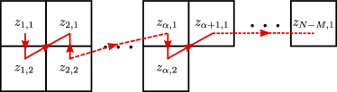
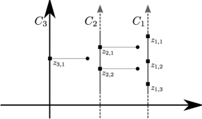
we recover (19) when $\xi=(n-m,m)$, i.e. a two-rows diagram with $\xi^{1}=\xi^{2}=\ldots=\xi^{n-m}=2,\xi^{n-m+1}=1,\ldots,\xi^{n}=1$. To see this it is enough to perform the change of variables $z_{\alpha,j}\to iz_{A}/\bar{c}$, where $A=1,\ldots,n$, with the ordering depicted in Fig. S1 (Left). Note that contours change as given in the text, where we have also distinguished contours for variables with the same index $\alpha$ (which is immaterial since no poles are encountered when bringing them together).

We will now show that, as for the bosonic case Borodin and Corwin (2014) where all $\xi^{\alpha}=1$, this expression is equivalent to the spectral expansion (Replica trick and nested-Bethe ansatz. —) in the text, into string solutions of the Bethe Ansatz equations. We use the notations of and extend the method to the case of a general symmetry. Starting from $z_{1,1}$ and the contour $C_{1}$, we recursively move all the contours to the leftmost $C_{n_{C}(\xi)}$. While displacing the contours, all the residues of the first product in (S46) have to be collected: they produce a hierarchy of additional terms with fewer integration variables $z_{\alpha_{k},i_{k}}$, which are the ending points of a sequence of residues $z_{\alpha_{1},i_{1}}=z_{\alpha_{2},i_{2}}+1=z_{\alpha_{3},i_{3}}+2=\ldots=z_{\alpha_{k},i_{k}}+k-1$.

Figure S1: Left – Sketch of the top-bottom/left-right filling of variables for a two-rows Young diagram. The ordering of the variables is represented by the arrows. Right – Structure of the poles (black disks) at $z_{\alpha,i}+1$ with $\alpha>1$ when integrating the variables $z_{1,j}$, $j=1,2,3$ with $\xi=(321)$.

Each of these terms is characterized by the length $\chi_{\alpha}=k$ of these sequences, that we arrange in another diagram of size $n$: $\chi=(\chi_{1}\chi_{2}\ldots)$. A filling $\phi$ of the diagram $\chi$ corresponds to assign the variables $z_{\alpha,i}$ to each box thus fixing the sequence of residues. For instance for $\xi=(42)$ and $\chi=(321)$ one possible filling is:

(S49)

and in general we indicate as $z_{\phi_{i,j}}$ the variable in the box at row $i$ and column $j$ of the filling $\phi$. In order to have a non-vanishing residue, each index $\alpha$ has to grow strictly along each row. This restricts the possible diagrams $\chi$ to those satisfying $\chi\prec\xi$, meaning that either $\xi\equiv\chi$ or $\xi_{i}>\chi_{i}$, where $i$ is the smallest index where they differ. Then Eq. (S46) is expanded as a sum over all the elements of the set of allowed fillings $\Phi(\chi)$ of the diagrams $\chi\prec\xi$

$$\mathcal{Z}_{\xi}(T)=\prod_{\alpha=1}^{n_{C}(\xi)}\frac{1}{\xi^{\alpha}!}\sum_{\stackrel{{\scriptstyle\chi\prec\xi}}{{\chi=1^{a_{1}}2^{a_{2}}\ldots}}}\frac{1}{a_{1}!a_{2}!\cdots}\sum_{\phi\in\Phi(\chi)}\int\cdots\int\prod_{p=1}^{n_{R}(\chi)}{\frac{dz_{\phi_{p,\chi_{p}}}}{2\pi i}}\\ \times\operatorname{Res}_{\phi}\left[\left(\prod_{\alpha<\beta}\prod_{i,j}\frac{z_{\alpha,i}-z_{\beta,j}}{z_{\alpha,i}-z_{\beta,j}-1}\right)\left(\prod_{\alpha=1}^{n_{C}(\xi)}\prod_{i\neq j}^{\xi^{\alpha}}(z_{\alpha,i}-z_{\alpha,j})\right)F(\{z\})\right]\;.$$ (S50)

The multiplicities $a_{k}$ are the number of indexes $\alpha$ such that $\chi_{\alpha}=k$ and avoid the overcounting when a diagram $\chi$ has multiple rows of the same length, i.e. multiple strings of the same length. The expression $\operatorname{Res}_{\phi}[G(\{z\})]$ entails the iterative computation of all the residues at $z_{\phi_{k,l}}=z_{\phi_{k,l+1}}+1$ for $k=1,\ldots,n_{R}(\chi)$ and $l=1,\ldots,\chi_{k}-1$, obtaining finally a function of the rightmost variables $z_{\phi_{p,\chi_{p}}}$ in each row of $\phi$. Now we consider the relabeling

$$(z_{\phi_{1,1}},z_{\phi_{1,2}},\ldots,z_{\phi_{1,\chi_{1}}}) \to(y_{\chi_{1}},y_{\chi_{1}-1},\ldots,y_{1})$$ (S51)

$$(z_{\phi_{2,1}},z_{\phi_{2,2}},\ldots,z_{\phi_{2,\chi_{2}}}) \to(y_{\chi_{1}+\chi_{2}},y_{\chi_{1}+\chi_{2}-1},\ldots,y_{\chi_{1}+1})$$ (S52)

$$\vdots$$ (S53)

which we indicate shortly as $z_{\alpha,i}=y_{\phi^{\ast}(\alpha,i)}$; this defines implicitly, for each $\phi$, the mapping $\phi^{\ast}:(\alpha,i)\to\{1,\ldots,n\}$. We also label the final variables $w_{j}=y_{\chi_{1}+\ldots+\chi_{j-1}+1}$ for $1\leq j\leq n_{R}(\chi)$. For instance, for the filling $\phi$ considered in (S49)

$$\raisebox{-42.67912pt}{ \includegraphics[keepaspectratio={true},height=32.52017pt]{relabeling}}\;.$$ (S54)

In this way, we arrive at

$$\mathcal{Z}_{\xi}(T)=\prod_{\alpha=1}^{n_{C}(\xi)}\frac{1}{\xi^{\alpha}!}\sum_{\stackrel{{\scriptstyle\chi\prec\xi}}{{\chi=1^{a_{1}}2^{a_{2}}\ldots}}}\frac{1}{a_{1}!a_{2}!\cdots}\sum_{\phi\in\Phi(\chi)}\int\cdots\int\prod_{p=1}^{n_{R}(\chi)}{\frac{dw_{p}}{2\pi i}}\\ \times\operatorname{Res}_{\chi}\left[\left(\prod_{\alpha<\beta}\prod_{i,j}\frac{y_{\phi^{\ast}(\alpha,i)}-y_{\phi^{\ast}(\beta,j)}}{y_{\phi^{\ast}(\alpha,i)}-y_{\phi^{\ast}(\beta,j)}-1}\right)\left(\prod_{\alpha=1}^{n_{C}(\xi)}\prod_{i\neq j}^{\xi^{\alpha}}(y_{\phi^{\ast}(\alpha,i)}-y_{\phi^{\ast}(\alpha,j)})\right)F(\{y_{\phi^{\ast}}\})\right]\;.$$ (S55)

Notice that in this expression we replaced $\operatorname{Res}_{\phi}$ with $\operatorname{Res}_{\chi}$, since when written in the variables $y$’s, the sequence of residues to be computed does not depend on the specific filling $\phi$ but only on the diagram $\chi$. Now, we observe that if the constraint $\chi\prec\xi$ is removed and the sum is extended over arbitrary filling $\phi$ of the variables $y$’s in $\chi$, the result does not change. This because the added terms will have a vanishing residue. For instance, if in (S54) one exchanges $z_{2,1}$ and $z_{1,1}$ there is no associated pole in the first factor. In this case the sum over all possible fillings $\phi$ without constraints, amounts to a sum over all permutations of the variables $y$. Hence, the above expression can be replaced by a symmetrization over the variables $y$, and we arrive at

$$\mathcal{Z}_{\xi}(T)=\prod_{\alpha=1}^{n_{C}(\xi)}\frac{1}{\xi^{\alpha}!}\sum_{\chi=1^{a_{1}}2^{a_{2}}\ldots}\frac{n!}{a_{1}!a_{2}!\cdots}\int\cdots\int\prod_{p=1}^{n_{R}(\chi)}{\frac{dw_{p}}{2\pi i}}\\ \times\operatorname{Res}_{\chi}\left[\operatorname{sym}_{y}W_{0}(\{y\})\right]\;.$$ (S56)

with $W_{0}(\{y\})$ defined as

$$W_{0}(\{y\})\equiv\left(\prod_{\alpha<\beta}\prod_{i,j}\frac{y_{\phi^{\ast}(\alpha,i)}-y_{\phi^{\ast}(\beta,j)}}{y_{\phi^{\ast}(\alpha,i)}-y_{\phi^{\ast}(\beta,j)}-1}\right)\left(\prod_{\alpha=1}^{n_{C}(\xi)}\prod_{i\neq j}^{\xi^{\alpha}}(y_{\phi^{\ast}(\alpha,i)}-y_{\phi^{\ast}(\alpha,j)})\right)F(\{y_{\phi^{\ast}}\})=\\ =\left(\prod_{k\neq l}\frac{y_{k}-y_{l}}{y_{k}-y_{l}-1}\right)\left(\prod_{k>l}\frac{y_{k}-y_{l}-1}{y_{k}-y_{l}}\right)\left(\prod_{\alpha=1}^{n_{C}(\xi)}\prod_{i>j}^{\xi^{\alpha}}(y_{\phi^{\ast}_{\xi}(\alpha,i)}-y_{\phi^{\ast}_{\xi}(\alpha,j)})(y_{\phi^{\ast}_{\xi}(\alpha,j)}-y_{\phi^{\ast}_{\xi}(\alpha,i)}-1)\right)F(\{y_{\phi^{\ast}_{\xi}}\})\;.$$ (S57)

Here, in the first line, because of the symmetrization the filling $\phi$ of $\xi$ is arbitrary. In the second line of (S57), and everywhere below, we choose the “canonical” one $\phi\equiv\phi_{\xi}$ satisfying $\phi^{\ast}_{\xi}(\alpha,j+1)-\phi^{\ast}_{\xi}(\alpha,j)=1$, and increasing with $\alpha$ (see (S61) below for an explicit example), in agreement with the ordering in Fig. S1 – note: do not confuse the filling $\phi_{\xi}$ of the diagram $\xi$, used to define $W_{0}$ in (S57), with the the filling of $\chi$ in (S54). The only term singular when evaluating the residue in this expression is the first one, which is already symmetric over $y$’s, and can be expressed as a determinant of a $n_{R}(\chi)\times n_{R}(\chi)$ matrix Borodin and Corwin (2014)

$$\operatorname{Res}_{\chi}\left[\prod_{k\neq l}\frac{y_{k}-y_{l}}{y_{k}-y_{l}-1}\right]=\det\left(\frac{1}{w_{i}+\chi_{i}-w_{j}}\right)_{i,j=1}^{n_{R}(\chi)}\;.$$ (S58)

The remaining term is not singular upon evaluation of these residues and we just need to insert the variables obtaining our main result:

Proposition: —

$$\mathcal{Z}_{\xi}(T)=\prod_{\alpha=1}^{n_{C}(\xi)}\frac{1}{\xi^{\alpha}!}\sum_{\chi=1^{a_{1}}2^{a_{2}}\ldots}\frac{n!}{a_{1}!a_{2}!\cdots}\int\cdots\int\prod_{p=1}^{n_{R}(\chi)}{\frac{dw_{p}}{2\pi i}}\\ \times\det\left(\frac{1}{w_{i}+\chi_{i}-w_{j}}\right)_{i,j=1}^{n_{R}(\chi)}\operatorname{Sub}_{\chi}\left[\operatorname{sym}_{y}W_{\xi}(\{y\})\right]\;.$$ (S59)

Here the operator $\operatorname{Sub}_{\chi}$ requires replacing $y_{i}=y_{i-1}+1$ for for $i\nin\{1,1+\chi_{1},1+\chi_{1}+\chi_{2},\ldots\,,1+\chi_{1}+\ldots+\chi_{n_{R}(\chi)-1}\}$ and considering the result as a function of $w_{j}=y_{1+\sum_{l=1}^{j-1}\chi_{l}}$, with $j=1,\ldots,n_{R}(\chi)$. The function $W_{\xi}(\{y\})$ contains the non-symmetric part of $W_{0}(\{y\})$ and is the only part depending on the choice of the diagram $\xi$:

$$W_{\xi}(\{y\})\equiv\left(\prod_{k>l}\frac{y_{k}-y_{l}-1}{y_{k}-y_{l}}\right)\left(\prod_{\alpha=1}^{n_{C}(\xi)}\prod_{i>j}^{\xi^{\alpha}}(y_{\phi^{\ast}_{\xi}(\alpha,i)}-y_{\phi^{\ast}_{\xi}(\alpha,j)})(y_{\phi^{\ast}_{\xi}(\alpha,j)}-y_{\phi^{\ast}_{\xi}(\alpha,i)}-1)\right)F(\{y_{\phi^{\ast}_{\xi}}\})\;.$$ (S60)

with $\phi_{\xi}$ the “canonical” filling associated to the diagram $\xi$.

Remarkably, all the other terms remain equal to the bosonic case. Finally, for the two-rows diagram $\xi=(n-m,m)$, Eq. (15) and (20) are recovered by the change of variables $w_{j}\to ik_{j}/\bar{c}-(m_{j}-1)/2$, $j=1,\ldots,n_{s}$, and in general $y_{A}\to i\mu_{A}/\bar{c}$ for $A=1,\ldots,n$, where each row of $\chi$ is identified with a string configuration, so that $m_{j}=\chi_{j}$ and $n_{s}=n_{R}(\chi)$. The substitutions in (S48) are finally applied. For instance, for $\xi=(42)$, we have the filling

$$\phi_{\xi}=\raisebox{-28.45274pt}{ \includegraphics[keepaspectratio={true},height=26.01613pt]{finalexample}}$$ (S61)

and we obtain

$$\prod_{\alpha,i>j}(y_{\phi^{\ast}_{\xi}(\alpha,i)}-y_{\phi^{\ast}_{\xi}(\alpha,j)})(y_{\phi^{\ast}_{\xi}(\alpha,j)}-y_{\phi^{\ast}_{\xi}(\alpha,i)}-1)=[(y_{2}-y_{1})(y_{1}-y_{2}-1)][(y_{4}-y_{3})(y_{3}-y_{4}-1)]=\frac{h(\mu_{1,2})h(\mu_{3,4})}{\bar{c}^{4}}\;.$$ (S62)

To avoid confusion, we remark that Eq. (S61) is used to define $W_{\xi}$ in (S60). Only after the symmetrization over $y$ in (S59) has been performed, one must carry on the replacement $\operatorname{Sub}_{\chi}$ corresponding to each diagram $\chi$, as indicated above, which is equivalent to injecting the string eigenstates.

In general, the determinant in (S59) produces the term $\Phi(\mathbf{k},\mathbf{m})$ in (15), while the first and second factor in (S60) give respectively the denominator and the numerator in (20).

V GGE partition function

We derive a Fredholm determinant form for the generalized generating function, defined as

$$J_{\bm{\beta}}(u,t)=\sum_{n\geq 0}\frac{(-u)^{n}}{n!}\mathcal{Z}_{n}^{\bm{\beta}}(t)\;.$$ (S63)

where, in this work, we introduced the GGE partition function as the following sum restricted over bosonic states (i.e. fully symmetric)

$$\mathcal{Z}_{n}^{\bm{\beta}}(t)=\sum_{\mu\text{\tiny, bosonic}}\frac{|\psi_{\mu}(0)|^{2}}{||\mu||^{2}}e^{-tA_{2}+\sum_{p\geq 1}\beta_{p}A_{p}}=\sum_{n_{s}=1}^{n}\frac{n!\bar{c}^{n}}{n_{s}!(2\pi\bar{c})^{n_{s}}}\sum_{(m_{1},..m_{n_{s}})_{n}}\prod_{j=1}^{n_{s}}\int_{-\infty}^{+\infty}\frac{dk_{j}e^{-tA_{2}+\sum_{p\geq 1}\beta_{p}A_{p}}}{m_{j}}\Phi(\mathbf{k},\mathbf{m})\;.$$ (S64)

the charges being defined as $A_{p}=\sum_{j}\mu_{j}^{p}$, and the second equality uses the decomposition over string states valid in the large $L$ limit. It is thus a generalization of the bosonic partition sum of the fixed endpoint directed polymer studied in Calabrese et al. (2010); dotsenko . Here it appears naturally in the non-symmetric problem, and its calculation generalizes the one of Ref. Calabrese et al. (2010). Note that in (S63) we have defined $\mathcal{Z}_{n}^{\bm{\beta}}(t)=1$, which we find to be a consistent analytical continuation of the GGE partition sum to $n=0$.

After the insertion of the string ansatz, the charges take the form $A_{p}=\sum_{j=1}^{n_{s}}\tilde{A}_{p}(k_{j},m_{j})$ with

$$\tilde{A}_{1}(k,m) =km\;,$$ (S65)

$$\tilde{A}_{2}(k,m) =mk^{2}+\frac{1}{12}(m-m^{3})\bar{c}^{2}\;,$$ (S66)

$$\tilde{A}_{3}(k,m) =\frac{km}{4}\left(4k^{2}+(1-m^{2})\bar{c}^{2}\right)\;.$$ (S67)

$$\tilde{A}_{4}(k,m) =mk^{4}+\frac{1}{2}\bar{c}^{2}k^{2}m\left(1-m^{2}\right)+\frac{1}{240}\bar{c}^{4}m\left(3m^{4}-10m^{2}+7\right)$$ (S68)

Exchanging in (S63) the sum over $n_{s}$ and the one over $n$, we can rewrite it as

$$J_{\bm{\beta}}(u,t)=\sum_{n_{s}=0}^{\infty}\frac{1}{n_{s}!}\mathcal{Z}^{(n_{s})}_{\bm{\beta}}(u,t)$$ (S69)

where the partition function with a fixed number of strings has been introduced

$$\mathcal{Z}^{(n_{s})}_{\bm{\beta}}(u,t)=\sum_{m_{1}\ldots m_{n_{s}}=1}^{\infty}\frac{(-u\bar{c})^{\sum_{j}m_{j}}}{(2\pi\bar{c})^{n_{s}}}\int_{\mathbb{R}^{n_{s}}}\left[\prod_{j=1}^{n_{s}}\frac{dk_{j}e^{-t\tilde{A}_{2}(k_{j},m_{j})+\sum_{p\geq 1}\beta_{p}\tilde{A}_{p}(k_{j},m_{j})}}{m_{j}}\right]\Phi(\mathbf{k},\mathbf{m})\;.$$ (S70)

To proceed further we rewrite this expression introducing the determinant of a $n_{s}\times n_{s}$ matrix

$$\det\left(\frac{1}{2ik_{i}-2ik_{j}+\bar{c}(m_{i}+m_{j})}\right)\prod_{j=1}^{n_{s}}(2\bar{c}m_{j})=\Phi(\mathbf{k},\mathbf{m})$$ (S71)

which follows by the Cauchy-determinant formula Schechter (1959), and leads to

$$\mathcal{Z}^{(n_{s})}_{\bm{\beta}}(u,t)=2^{n_{s}}\sum_{m_{1}\ldots m_{n_{s}}=1}^{\infty}\int_{\mathbb{R}^{n_{s}}}\left[\prod_{j=1}^{n_{s}}\frac{dk_{j}(-u\bar{c})^{m_{j}}e^{-t\tilde{A}_{2}(k_{j},m_{j})+\sum_{p\geq 1}\beta_{p}\tilde{A}_{p}(k_{j},m_{j})}}{2\pi}\right]\det\left(\frac{1}{2ik_{i}-2ik_{j}+\bar{c}(m_{i}+m_{j})}\right)\;.$$ (S72)

We now employ the Laplace expansion for the determinant

$$\det\left(\frac{1}{2ik_{i}-2ik_{j}+\bar{c}(m_{i}+m_{j})}\right)=\sum_{P}(-1)^{\sigma_{P}}\prod_{j=1}^{n_{s}}\frac{1}{2ik_{j}-2ik_{P_{j}}+\bar{c}(m_{j}+m_{P_{j}})}=\\ =\sum_{P}(-1)^{\sigma_{P}}\int_{v_{j}>0}\prod_{j}dv_{j}e^{-v_{j}(2ik_{j}-2ik_{P_{j}}+\bar{c}(m_{j}+m_{P_{j}}))}=\sum_{P}(-1)^{\sigma_{P}}\int_{v_{j}>0}\prod_{j}dv_{j}e^{-2ik_{j}(v_{j}-v_{P_{j}})-\bar{c}m_{j}(v_{j}+v_{P_{j}})}$$ (S73)

where in the last equality we exchanged $P$ with $P^{-1}$ taking into account that they have the same parity. Replacing (S73) inside (S72) we obtain

$$\mathcal{Z}^{(n_{s})}_{\bm{\beta}}(u,t)=\prod_{j=1}^{n_{s}}\int_{v_{j}>0}\det{\mathcal{K}}^{\bm{\beta}}_{u}(v_{i},v_{j}).$$ (S74)

with the Kernel

$${\mathcal{K}}^{\bm{\beta}}_{u}(v_{1},v_{2})=\int_{-\infty}^{\infty}\frac{dk}{2\pi}\sum_{m=1}^{\infty}2(-\bar{c}u)^{m}e^{-t\tilde{A}_{2}(k,m)+\sum_{p\geq 1}\beta_{p}\tilde{A}_{p}(k,m)}e^{-2ik(v_{1}-v_{2})-\bar{c}m(v_{1}+v_{2})}\;.$$ (S75)

From this it follows that

$$J_{\bm{\beta}}(u,t)=\operatorname{Det}(1+\Pi_{0}{\mathcal{K}}^{\bm{\beta}}_{u}\Pi_{0})$$ (S76)

in terms of a Fredholm determinant, where $\Pi_{s}$ is the projector on $[s,\infty)$.

VI Moments from generating function

As discussed in the text we expand the expressions for $\Lambda_{n,m}$ for $m=1,2,3$ in the conserved charges of the model $A_{p}$. We display here their full expression for $m=1,2$ and only the leading order in $1/n$ for $m=3$:

$$\Lambda_{n,1}=\frac{1}{n(n-1)}\left(nA_{2}-A_{1}^{2}+\frac{n^{2}(n^{2}-1)}{12}\bar{c}^{2}\right)=\frac{A_{1}^{2}}{n}+(A_{1}^{2}-A_{2})+O(n)\;,$$ (S77a)

$$\Lambda_{n,2}=\frac{(n^{2}-1)n(5n-6)\bar{c}^{4}}{720}-\frac{(A_{1}^{2}-nA_{2})\bar{c}^{2}}{6}+\frac{4(n-1)A_{3}A_{1}+(n^{2}-3n+3)A_{2}^{2}-(n-1)nA_{4}+A_{1}^{4}-2nA_{2}A_{1}^{2}}{(n-3)(n-2)(n-1)n}=$$ (S77b)

$$\hfill=\frac{1}{6n}(4A_{1}A_{3}-A_{1}^{4}-3A_{2}^{2})\;,+\frac{1}{36}(12A_{1}^{2}A_{2}+20A_{1}A_{3}-11A_{1}^{4}-15A_{2}^{2}-6A_{4})-\frac{A_{1}^{2}}{6}\bar{c}^{2}+O(n)$$ (S77c)

$$\begin{multlined}\Lambda_{n,3}=\frac{1}{120n}\left[-10\left(A_{1}^{4}-4A_{3}A_{1}+3A_{2}^{2}\right)\bar{c}^{2}+A_{1}^{6}-20A_{3}A_{1}^{3}+15\left(A_{2}^{2}+2A_{4}\right)A_{1}^{2}+\right.\\ \left.+\left(24A_{5}-60A_{2}A_{3}\right)A_{1}+10\left(3A_{2}^{3}-6A_{4}A_{2}+4A_{3}^{2}\right)\right]+O(n^{0})\;.\end{multlined}\Lambda_{n,3}=\frac{1}{120n}\left[-10\left(A_{1}^{4}-4A_{3}A_{1}+3A_{2}^{2}\right)\bar{c}^{2}+A_{1}^{6}-20A_{3}A_{1}^{3}+15\left(A_{2}^{2}+2A_{4}\right)A_{1}^{2}+\right.\\ \left.+\left(24A_{5}-60A_{2}A_{3}\right)A_{1}+10\left(3A_{2}^{3}-6A_{4}A_{2}+4A_{3}^{2}\right)\right]+O(n^{0})\;.$$ (S77f)

Using the GGE partition function in (S64), we can rewrite

$$\Theta_{n,m}(t)=\Lambda_{n,m}(\{\partial_{p}\})[\mathcal{Z}_{n}^{\bm{\beta}}(t)]$$ (S78)

where we replaced in $\Lambda_{n,m}$ the charges $A_{p}\to\partial_{p}$ computed setting all $\beta$’s to zero afterwards. We immediately see that the first expression (S77a) for $\Lambda_{n,1}$ leads to equation (16) in the text, valid for any $n$, using the equivalence $\partial_{2}\equiv-\partial_{t}$ and replacing $A_{1}^{2}\to\frac{n}{2t}$ which comes from the STS (see below). Note also that in the limit $n\to 0$ we will be allowed to discard in the Taylor expansion as written in (S77a-S77f), the terms formally of order $O(n^{0})$ and higher (not written for $m=3$), since (i) we have checked that they all contain derivatives acting on $\mathcal{Z}_{n}$ and (ii) $\mathcal{Z}_{n}^{\bm{\beta}}(t)\to 1$ when $n\to 0$ (see above).

The above expressions can be further simplified employing the STS symmetry, manifested here as the invariance of (S64) under the shift of all rapidities $\mu_{j}\to\mu_{j}+k$ for an arbitrary constant $k$. Such symmetry was used in e.g. Appendix of Ref. flat in presence of charges $A_{1},A_{2}$ only. Here we extend the analysis to the enlarged context of the GGE partition sum, which contains all charges $A_{p}$. Since under the shift ($A_{0}\equiv n$)

$$A_{p}\to A_{p}+\sum_{q=1}^{p}\binom{p}{q}A_{p-q}k^{q}$$ (S79)

at the order $O(k)$ in (S64), we obtain the equality, valid for arbitrary $\bm{\beta}$

$$\left[-2t\partial_{1}+n\beta_{1}+\sum_{p=2}^{\infty}p\beta_{p}\partial_{p-1}\right]\mathcal{Z}_{n}^{\bm{\beta}}(t)=0\;.$$ (S80)

By expansion order by order in $\bm{\beta}$, one obtains an infinite list of equalities involving conserved charges, that can be generated easily by

$$\langle\left[-2tA_{1}+\sum_{p=1}^{\infty}pA_{p-1}\partial_{A_{p}}\right]q(\{A\})\rangle~{}=0\;.$$ (S81)

where $q(\{A\})$ is an arbitrary polynomial in the $A_{p}$. Here, these identities are understood as inserted in the integral (15) over string momenta, which is denoted here as $\langle\ldots\rangle$. Equivalently, the charges are afterwards replaced by derivatives applied to $\mathcal{Z}_{n}^{\bm{\beta}}(t)$ as in (S78). Varying the choice of $q(\{A\})$, we obtain for instance

$$\langle A_{1}^{2k+1}\rangle=0,\qquad\langle A_{1}^{2k}\rangle=\frac{n^{k}(2k-1)!!}{2^{k}t^{k}},\quad\langle A_{1}A_{3}\rangle=\frac{3\langle A_{2}\rangle}{2t}\;.$$ (S82)

where the last equality goes beyond the standard use of STS (in e.g. Ref. flat ).

Thanks to these identities, the limit $n\to 0$ can be taken in (S77). For $m=1,2$ only $A_{2}$ survives, that, being the energy, can be replaced according to $\partial_{2}\equiv-\partial_{t}$. Then using (S82), Eqs. (S77a) and (S77c) lead respectively to (16) and (22) in the text, using that

$$\frac{1}{n}\partial_{2}^{p}\mathcal{Z}_{n}^{\bm{\beta}}(t)|_{\bm{\beta}=0}=\frac{1}{n}(-\partial_{t})^{p}{\cal Z}_{n}(t)\xrightarrow{n\to 0}(-\partial_{t})^{p}\overline{\ln Z_{\eta}(0;0|t)}\;.$$ (S83)

For $m\geq 3$, higher conserved charges are involved and the moments are not simply related to the free-energy distribution. For instance for $m=3$ after using STS we find that we can replace:

$$\ \Lambda_{n,3}\to\frac{1}{n}\left[\frac{\bar{c}^{2}A_{2}}{2t}-\frac{\bar{c}^{2}A_{2}^{2}}{4}-\frac{3A_{2}^{2}}{4t}+\frac{A_{2}^{3}}{4}+\frac{A_{3}^{2}}{3}+\frac{A_{4}}{2t}-\frac{A_{2}A_{4}}{2}\right]$$ (S84)

with no further simplification. Using (S78) the final result for $\overline{p_{\eta}(t)^{3}}$ is thus a linear combination of

$$\rho_{i_{1},\ldots,i_{k}}\equiv\left.\lim_{n\to 0}\partial_{i_{1}}\ldots\partial_{i_{k}}\frac{\mathcal{Z}_{n}^{\bm{\beta}}(t)-1}{n}\right|_{\bm{\beta}=0}\;.$$ (S85)

where $\partial_{i_{1}}\equiv\partial_{\beta_{i_{1}}}$. The $\rho_{i_{1},\ldots,i_{k}}$ can then be expressed as derivatives acting on the Fredholm determinant expression(S76). To see this, we write it as a Mellin transform

$$\mathcal{Z}_{n}^{\bm{\beta}}(t)=\int_{0}^{\infty}dy\tilde{\mathcal{Z}}_{\bm{\beta}}(y,t)y^{n}\;,$$ (S86)

which can be inserted in (S63) to give

$$J_{\bm{\beta}}(u,t)=\int_{0}^{\infty}dy\tilde{\mathcal{Z}}_{\bm{\beta}}(y,t)e^{-uy}\;.$$ (S87)

with $J_{\bm{\beta}}(0,t)=1$. This shows that $\tilde{\mathcal{Z}}_{\bm{\beta}}(y,t)$ can be equivalently defined as the inverse Laplace transform of $J_{\bm{\beta}}(u,t)$. Inserting (S86) in (S85) and taking the limit $n\to 0$, we obtain for $k>0$

$$\rho_{i_{1},\ldots,i_{k}} = \partial_{i_{1}}\ldots\partial_{i_{k}}\int_{0}^{\infty}dy\tilde{\mathcal{Z}}_{\bm{\beta}}(y,t)\ln y=\partial_{i_{1}}\ldots\partial_{i_{k}}\int_{0}^{\infty}\frac{du}{u}\left(e^{-u}-J_{\bm{\beta}}(u,t)\right)=-\int_{0}^{\infty}\frac{du}{u}\partial_{i_{1}}\ldots\partial_{i_{k}}J_{\bm{\beta}}(u,t)\;$$ (S88)

$$= -\int_{0}^{\infty}\frac{du}{u}\partial_{i_{1}}\ldots\partial_{i_{k}}\operatorname{Det}(1+\Pi_{0}{\mathcal{K}}^{\bm{\beta}}_{u}\Pi_{0}).$$

Derivatives of a FD are easily evaluated, for instance for $k=2$ one obtains

$$\partial_{a}\partial_{b}J_{\bm{\beta}}(u,t)=\left[\operatorname{Tr}[(1+{\mathcal{K}}^{\bm{\beta}}_{u})^{-1}\partial_{a}\partial_{b}{\mathcal{K}}^{\bm{\beta}}_{u}]+\operatorname{Tr}[(1+{\mathcal{K}}^{\bm{\beta}}_{u})^{-1}\partial_{a}{\mathcal{K}}^{\bm{\beta}}_{u}]\operatorname{Tr}[(1+{\mathcal{K}}^{\bm{\beta}}_{u})^{-1}\partial_{b}{\mathcal{K}}^{\bm{\beta}}_{u}]+\right.\\ \left.-\operatorname{Tr}[(1+{\mathcal{K}}^{\bm{\beta}}_{u})^{-1}\partial_{a}{\mathcal{K}}^{\bm{\beta}}_{u}(1+{\mathcal{K}}^{\bm{\beta}}_{u})^{-1}\partial_{b}{\mathcal{K}}^{\bm{\beta}}_{u}]\right]\operatorname{Det}(1+\Pi_{0}{\mathcal{K}}^{\bm{\beta}}_{u}\Pi_{0})\;.$$ (S89)

The derivatives with respect to the Lagrange multiplier $\bm{\beta}$, once applied to the kernel ${\mathcal{K}}^{\bm{\beta}}_{u}$ can be converted, using (S75) and (S65), into a combination of derivatives with respect to $v_{1},v_{2}$, e.g.

$$\partial_{1}{\mathcal{K}}^{\bm{\beta}}_{u}(v_{1},v_{2}) =\frac{\partial_{v_{1}-v_{2}}\partial_{v_{1}+v_{2}}{\mathcal{K}}^{\bm{\beta}}_{u}(v_{1},v_{2})}{2i\bar{c}}=-\frac{i(\partial_{v_{1}}^{2}-\partial_{v_{2}}^{2}){\mathcal{K}}^{\bm{\beta}}_{u}(v_{1},v_{2})}{8\bar{c}}$$ (S90)

$$\partial_{3}{\mathcal{K}}^{\bm{\beta}}_{u}(v_{1},v_{2}) =\frac{i(\partial_{v_{1}}^{4}-\partial_{v_{2}}^{4}){\mathcal{K}}^{\bm{\beta}}_{u}(v_{1},v_{2})}{64\bar{c}}+\frac{\bar{c}^{2}\partial_{1}{\mathcal{K}}^{\bm{\beta}}_{u}(v_{1},v_{2})}{4}\;.$$ (S91)

and more generally, from (S75)

$$\partial_{j}{\mathcal{K}}^{\bm{\beta}}_{u}(v_{1},v_{2})=\tilde{A}_{p}(k=\frac{i}{2}\partial_{v_{1}-v_{2}},m=-\frac{1}{\bar{c}}\partial_{v_{1}+v_{2}})\;.$$ (S92)

These formulas can be iterated in case of multiple derivatives, leading to explicit but lengthy expressions. The limit $\bm{\beta}\to 0$ can now be taken safely and we then have to deal only with the standard kernel ${\mathcal{K}}_{u}\equiv{\mathcal{K}}^{\bm{\beta}=0}_{u}$, as given in Ref. Calabrese et al. (2010). The calculation at arbitrary time by this method is possible but very demanding.

Let us now show how the asymptotics at large time simplifies. We set $\lambda^{3}=\bar{c}^{2}t/4$ and introduce $s$ by $e^{-\lambda s}=(u\bar{c})e^{-\frac{\lambda^{3}}{3}}$. Moreover, we rescale $k\to k\bar{c}/\lambda$ and $v_{1,2}\to\lambda v_{1,2}/\bar{c}$, so that ${\mathcal{K}}_{u}(v_{1},v_{2})\to\lambda{\mathcal{K}}_{s}(v_{1},v_{2})/\bar{c}$, because of the integration measure, and we obtain finally the $\lambda\to\infty$ limit

$${\mathcal{K}}_{s}^{\infty}(v_{1},v_{2})=-\int_{-\infty}^{\infty}\frac{dk}{2\pi}\int_{0}^{\infty}dy\operatorname{Ai}(y+k^{2}+s+v_{1}+v_{2})e^{-ik(v_{1}-v_{2})}=-2^{1/3}K_{\operatorname{Ai}}(2^{1/3}(v_{1}+s/2),2^{1/3}(v_{2}+s/2))\;.$$ (S93)

with the Airy Kernel defined as

$$K_{\operatorname{Ai}}(x,y)=\int_{0}^{\infty}dy\operatorname{Ai}(v_{1}+y)\operatorname{Ai}(v_{2}+y)=\frac{\operatorname{Ai}(v_{1})\operatorname{Ai}^{\prime}(v_{2})-\operatorname{Ai}^{\prime}(v_{1})\operatorname{Ai}(v_{2})}{v_{1}-v_{2}}\;.$$ (S94)

In this regime, the Fredholm determinant can be computed efficiently numerically following Bornemann (2009).

Let us show how to obtain the leading large time behavior on the example of $m=3$. First one sees that one can decompose the charges (S65) as:

$$\tilde{A}_{2}(k,m)=\hat{A}_{2}(k,m)+\frac{\bar{c}^{2}}{12}m\;,$$ (S95)

$$\tilde{A}_{3}(k,m)=\hat{A}_{3}(k,m)+\frac{\bar{c}^{2}}{4}\tilde{A}_{1}(k,m)\;,$$ (S96)

$$\tilde{A}_{4}(k,m)=\hat{A}_{4}(k,m)+\frac{7\bar{c}^{4}}{240}m+\frac{\bar{c}^{2}}{2}\hat{A}_{2}(k,m)$$ (S97)

and $\tilde{A}_{1}(k,m)=\hat{A}_{1}(k,m)$, where $\hat{A}_{p}(k,m)$ is the homogeneous part, i.e. $\hat{A}_{p}(\frac{k\bar{c}}{\lambda},m)=\lambda^{-(p+1)}\hat{A}_{p}(k\bar{c},\lambda m)$ under the rescaling $k\to k\bar{c}/\lambda$. Thus in (S84) one can formally decompose the charges as:

$$A_{2}=\hat{A}_{2}+\frac{\bar{c}^{2}n}{12}\quad,\quad A_{3}=\hat{A}_{3}+\frac{\bar{c}^{2}A_{1}}{4}\quad,\quad A_{4}=\hat{A}_{4}+\frac{7\bar{c}^{4}n}{240}+\frac{\bar{c}^{2}\hat{A}_{2}}{2}$$ (S98)

and the above analysis of the FD at large time shows that the hat charges scale as $\hat{A}_{p}\sim t^{-(p+1)/3}$, which we denote by ”normal” scaling, and ${\cal Z}_{n}/n$ scales as $t^{1/3}$. For example $A_{2}\mathcal{Z}_{n}/n\xrightarrow{n\to 0}-\partial_{t}\overline{\ln Z_{\eta}(0;0|t)}=\bar{c}^{2}/12+O(t^{-2/3})$ has “anomalous” scaling, while $\hat{A}_{2}\mathcal{Z}_{n}/n\xrightarrow{n\to 0}O(t^{-2/3})$ has “normal” scaling with time at large time.

Putting all together, in the limit $n\to 0$ we find:

$$\overline{p_{\eta}(t)^{3}}\simeq\frac{\bar{c}^{4}}{15t}-\frac{2\overline{\chi_{2}}\bar{c}^{8/3}}{9t^{5/3}}$$ (S99)

where the sub-leading term is obtained using (S98) in (S84). Then the term scaling as $t^{-5/3}$ gives at large times

$$\lim_{n\to 0}\left(\frac{3\hat{A}_{2}}{4t}-\frac{\hat{A}_{2}^{2}}{2}+\frac{\hat{A}_{1}\hat{A}_{3}}{6}\right)\frac{\bar{c}^{2}\mathcal{Z}_{n}}{n}=-\frac{\bar{c}^{4}}{12t}-\bar{c}^{2}\left(\frac{\partial_{t}}{t}+\frac{\partial_{t}^{2}}{2}\right)h(t)=-\frac{2\overline{\chi_{2}}\bar{c}^{8/3}}{9t^{5/3}}\;.$$ (S100)

VII conjecture for $\overline{\ln p_{\eta}(t)}$

In Doumerc relations between some discrete DP models and the eigenvalues of the GUE (and LUE) random matrix ensembles are discussed. For instance, calling $h_{k}$ the maximum energy of an ensemble of $k$ non-crossing paths of $\simeq N$ steps with nearest neighbor endpoints in a semi-discrete DP model, and $\lambda_{1}>\lambda_{2}$ the two largest eigenvalues of the GUE(N), it is stated that:

$$h_{1}=_{d}\lambda_{1}$$ (S101)

$$h_{2}-h_{1}=_{d}\lambda_{2}$$ (S102)

where $=_{d}$ denotes equality in law (where, for our purpose, we consider $N$ large). Under appropriate rescaling Borodin and Corwin (2014), universality then suggests that at large time for the continuum DP model:

$$\ln Z_{\eta}\simeq-\frac{\bar{c}^{2}t}{12}+\overline{\chi_{2}}(\bar{c}^{2}t)^{1/3}$$ (S103)

$$\ln\frac{Z^{(2)}_{\eta}(\epsilon)}{(2\epsilon)^{2}}-\ln Z_{\eta}\simeq-\frac{\bar{c}^{2}t}{12}+\overline{\chi^{\prime}_{2}}(\bar{c}^{2}t)^{1/3}$$ (S104)

where the limit of small $\epsilon$ is implicit, and we denote $Z_{\eta}\equiv Z_{\eta}(0;0|t)$. Here $\chi_{2}>\chi^{\prime}_{2}$ are the two largest eigenvalues of the GUE, scaled so that the largest one obeys the Tracy Widom cumulative distribution $F_{2}$. These equations imply:

$$\overline{\ln p_{\eta}(t)}=\overline{\ln\frac{Z^{(2)}_{\eta}(\epsilon)}{(2\epsilon)^{2}}}-2~{}\overline{\ln Z_{\eta}}\simeq-(\overline{\chi_{2}}-\overline{\chi^{\prime}_{2}})(\bar{c}^{2}t)^{1/3}\approx-1.9043(\bar{c}^{2}t)^{1/3}$$ (S105)

with $\overline{\chi_{2}}=-1.7710868$ and $\overline{\chi^{\prime}_{2}}=-3.6754$ (value given in TWNote ). We have obtained preliminary numerical support for this behavior delucaledou . This means that in typical disorder configurations $p_{\eta}(t)$ decreases (sub)-exponentially fast with time, while its moments are dominated by rare, but not so rare, disorder configurations. This is similar to the behavior of the probability $q_{\eta}(t)$ that a single DP does not cross a hard wall at $x=0$ studied in Gueudre , where it was found that $\overline{\ln q_{\eta}(t)}=-(\overline{\chi_{2}}-\overline{\chi_{4}})(\bar{c}^{2}t)^{1/3}\approx-1.49134(\bar{c}^{2}t)^{1/3}$ where $\chi_{4}$ is distributed according to the GSE TW distribution with $\overline{\chi_{4}}=-3.2624279$. Note that avoiding a second polymer (which itself wanders and competes for the same favorable regions of the random potential) is more restrictive in phase space for the DP than a hard wall, consistent with $\overline{\ln p_{\eta}(t)}<\overline{\ln q_{\eta}(t)}$ as we find.

References

- Huse et al. (1985) D. A. Huse, C. L. Henley, and D. S. Fisher, Phys. Rev. Lett. 55, 2924 (1985).
- Kardar and Zhang (1987) M. Kardar and Y.-C. Zhang, Phys. Rev. Lett. 58, 2087 (1987).
- Halpin-Healy and Zhang (1995) T. Halpin-Healy and Y.-C. Zhang, Physics reports 254, 215 (1995).
- Blatter et al. (1994) G. Blatter et al., Rev. Mod. Phys. 66, 1125 (1994).
- Lemerle et al. (1998) S. Lemerle et al., Phys. Rev. Lett. 80, 849 (1998).
- (6) A. M. Somoza, M. Ortuño and J. Prior, Phys. Rev. Lett. 99, 116602 (2007). A. Gangopadhyay, V. Galitski, M. Mueller, arXiv:1210.3726, Phys. Rev. Lett. 111, 026801 (2013). A. M. Somoza, P. Le Doussal, M. Ortuno, arXiv:1501.03612 (2015).
- (7) J. Bec, K. Khanin, arXiv:0704.1611, Phys. Rep. 447, 1-66, (2007).
- (8) T. Gueudré, A. Dobrinevski, J.P. Bouchaud, arXiv:1310.5114, Phys. Rev. Lett. 112, 050602 (2014).
- Hwa and Lässig (1996) T. Hwa and M. Lässig, Phys. Rev. Lett. 76, 2591 (1996).
- (10) J. Otwinowski and J. Krug, Phys. Biol. 11 056003 (2014).
- Kardar et al. (1986) M. Kardar, G. Parisi, and Y.-C. Zhang, Phys. Rev. Lett. 56, 889 (1986).
- (12) M. Prähofer and H. Spohn, Phys. Rev. Lett. 84, 4882 (2000); J. Baik and E. M. Rains, J. Stat. Phys. 100, 523 (2000).
- (13) T. Sasamoto and H. Spohn, Phys. Rev. Lett. 104, 230602 (2010); Nucl. Phys. B 834, 523 (2010); J. Stat. Phys. 140, 209 (2010).
- (14) G. Amir, I. Corwin, J. Quastel, Comm. Pure Appl. Math 64, 466 (2011). I. Corwin, arXiv:1106.1596.
- (15) P. Calabrese, M. Kormos and P. Le Doussal, EPL 107, 10011 (2014)
- Borodin and Corwin (2014) A. Borodin and I. Corwin, Prob. Theor. and Rel. Fields 158, 225 (2014), also arXiv:11114408v4, Remark 5.4.7 .
- (17) J. Ortmann, J. Quastel and D. Remenik arXiv:1407.8484 and arXiv:1501.05626.
- (18) M. Kardar, Nucl. Phys. B 290, 582 (1987).
- Calabrese et al. (2010) P. Calabrese, P. Le Doussal, and A. Rosso, EPL 90, 20002 (2010).
- (20) V. Dotsenko, EPL 90, 20003 (2010); J. Stat. Mech. P07010 (2010);
- (21) P. Calabrese and P. Le Doussal, Phys. Rev. Lett. 106, 250603 (2011) and J. Stat. Mech. (2012) P06001.
- (22) T. Imamura, T. Sasamoto, arXiv:1111.4634, Phys. Rev. Lett. 108, 190603 (2012); arXiv:1105.4659, J. Phys. A 44, 385001 (2011); and arXiv:1210.4278 J. Stat. Phys. 150, 908-939 (2013).
- (23) E. H. Lieb and W. Liniger, Phys. Rev. 130, 1605 (1963).
- (24) P. Calabrese and J.-S. Caux, Phys. Rev. Lett. 98, 150403 (2007); J. Stat. Mech. (2007) P08032.
- (25) T. Nattermann, I. Lyuksyutov and M. Schwartz, EPL 16 295 (1991), J. Toner and D.P. DiVicenzo, Phys. Rev. B 41, 632(1990). J. Kierfeld and T. Hwa, Phys. Rev. Lett. 77, 20, 4233 (1996).
- (26) T. Emig, M. Kardar, arXiv:cond-mat/0101247, Nucl. Phys. B 604 [FS] (2001) 479 (2001).
- (27) P. L. Ferrari, arXiv:math-ph/0402053, Comm. Math. Phys., 252 (2004), 77-109
- Karlin et al. (1959) S. Karlin, J. McGregor, et al., Pacific J. Math 9, 1141 (1959).
- Gessel and Viennot (1985) I. M. Gessel and X. G. Viennot, Adv. Math. 58, 300 (1985).
- Gessel and Viennot (1989) I. M. Gessel and X. G. Viennot, Determinants, paths, and plane partitions (1989) unpublished preprint.
- Wikipedia (2015) Wikipedia, “Lindström-gessel-viennot lemma,” (2015).
- (32) C.-N. Yang, Phys. Rev. Lett. 19, 1312 (1967). M. Gaudin Phys. Lett. A 24 55 (1967); for an introduction, see also Chapters 11-12 in The Bethe Wavefunction, M. Gaudin (Cambridge University Press, 2014) .
- Fulton and Harris (1991) W. Fulton and J. Harris, Representation theory: a first course, Vol. 129 (Springer, 1991).
- Note (1) See Supplemental Material at [URL] for mathematical details of calculations and techniques presented in the main text.
- (35) See Eqs.(S19) and (S22) in Note (1).
- Note (3) see C. H. Lun and J. Warren, arXiv:1506.09030 for a rigorous discussion about the existence of the coinciding-points limit. Note that the r.h.s. of (3) is delicate to define mathematically in each sample and in the limit of white noise disorder. However, we use it only in average sense.
- (37) E. Brunet and B. Derrida, Phys. Rev. E 61, 6789 (2000).
- Pozsgay et al. (2012) B. Pozsgay, W.-V. van Gerven Oei, and M. Kormos, J. Phys. A 45, 465007 (2012).
- (39) See Section IIIb in Note (1) for the details about the norms and section IIIc for the resummation in the case . .
- Macdonald (1995) I. G. Macdonald, Symmetric functions and Hall polynomials (New York, 1995).
- Fioretto and Mussardo (2010) D. Fioretto and G. Mussardo, New J. Phys. 12, 055015 (2010).
- TracyMathematical Tables and Other Aids to Computation and Widom (1994) C. A. Tracy and H. Widom, Comm. Math. Phys. 159, 151 (1994).
- Sutherland (1968) B. Sutherland, Phys. Rev. Lett. 20, 98 (1968).
- Note (2) A. Borodin and I. Corwin, manuscript in preparation, see also A. Borodin et al., arXiv:1308.3475 section 7.2.
- Schechter (1959) S. Schechter, Math. tables other aids comput., 73 (1959).
- Bornemann (2009) F. Bornemann, arXiv:0904.1581 (2009).
- (47) N. O’Connell, M. Yor, Elect. Comm. in Probab. 7 (2002) 1, Y. Doumerc, Lecture Notes in Math., 1832: 370 (2003), I. Corwin et al., arXiv:1110.3489v4.
- (48) see Fig.2 in Ref. TracyMathematical Tables and Other Aids to Computation and Widom (1994).
- (49) A. De Luca and P. Le Doussal, to be published.
- (50) see discussion around Eq. (43) in T. Gueudre, P. Le Doussal, arXiv:1208.5669, EPL 100 26006 (2012).
- Gessel and Viennot (1985) I. M. Gessel and X. G. Viennot, Advances in mathematics 58, 300 (1985).
- Yang (1967) C.-N. Yang, Physical Review Letters 19, 1312 (1967).
- Sutherland (1968) B. Sutherland, Physical Review Letters 20, 98 (1968).
- Pozsgay et al. (2012) B. Pozsgay, W.-V. van Gerven Oei, and M. Kormos, Journal of Physics A: Mathematical and Theoretical 45, 465007 (2012).
- Calabrese and Caux (2007) P. Calabrese and J.-S. Caux, Journal of Statistical Mechanics: Theory and Experiment 2007, P08032 (2007).
- Calabrese et al. (2010) P. Calabrese, P. Le Doussal, and A. Rosso, EPL (Europhysics Letters) 90, 20002 (2010).
- Borodin and Corwin (2014) A. Borodin and I. Corwin, Probability Theory and Related Fields 158, 225 (2014).
- Note (1) Borodin private communication.
- Schechter (1959) S. Schechter, Mathematical Tables and Other Aids to Computation , 73 (1959).
- (14) V. Dotsenko, EPL 90, 20003 (2010); J. Stat. Mech. P07010 (2010);
- (15) P. Calabrese and P. Le Doussal, Phys. Rev. Lett. 106, 250603 (2011) and J. Stat. Mech. (2012) P06001.
- (17) N. O’Connell, M. Yor, Elect. Comm. in Probab. 7 (2002) 1, Y. Doumerc, Lecture Notes in Math., 1832: 370 (2003), I. Corwin et al., arXiv:1110.3489v4.
- (19) see Fig.2 in Ref. TracyMathematical Tables and Other Aids to Computation and Widom (1994).
- (20) A. De Luca and P. Le Doussal, to be published.
- (21) see discussion around Eq. (43) in T. Gueudre, P. Le Doussal, arXiv:1208.5669, EPL 100 26006 (2012).