N-jettiness Subtractions for NNLO QCD Calculations
Abstract
We present a subtraction method utilizing the -jettiness observable, , to perform QCD calculations for arbitrary processes at next-to-next-to-leading order (NNLO). Our method employs soft-collinear effective theory (SCET) to determine the IR singular contributions of -jet cross sections for , and uses these to construct suitable -subtractions. The construction is systematic and economic, due to being based on a physical observable. The resulting NNLO calculation is fully differential and in a form directly suitable for combining with resummation and parton showers. We explain in detail the application to processes with an arbitrary number of massless partons at lepton and hadron colliders together with the required external inputs in the form of QCD amplitudes and lower-order calculations. We provide explicit expressions for the -subtractions at NLO and NNLO. The required ingredients are fully known at NLO, and at NNLO for processes with two external QCD partons. The remaining NNLO ingredient for three or more external partons can be obtained numerically with existing NNLO techniques. As an example, we employ our results to obtain the NNLO rapidity spectrum for Drell-Yan and gluon-fusion Higgs production. We discuss aspects of numerical accuracy and convergence and the practical implementation. We also discuss and comment on possible extensions, such as more-differential subtractions, necessary steps for going to N3LO, and the treatment of massive quarks.
Keywords:
QCD, NNLO calculations, hadron colliders1 Introduction
The precise knowledge of QCD corrections is a key ingredient for interpreting the data from collider experiments. In hadronic collisions, the inclusive QCD cross section for the production of a final state can, if the hard scale associated with is large enough, be obtained in terms of a perturbatively calculable partonic cross section convolved with parton distribution functions (PDFs).
Perturbative calculations performed using the leading order (LO) term in typically suffer from large theoretical uncertainties due to missing higher-order perturbative corrections. Often, next-to-leading order (NLO) is the first order at which the normalization and in some cases the shape of cross sections can be considered reliable. As such, this level of accuracy has become standard for comparing with data from the LHC. For some processes the experimental uncertainties are becoming so small, or the perturbative uncertainties at NLO are still so large, that next-to-next-to-leading order (NNLO) computations are called for.
For many important benchmark processes, the required virtual amplitudes are known at NNLO. However, as is well known, the computation of the full cross sections beyond leading order is complicated by infrared (IR) divergences – explicit divergences in virtual amplitudes, and divergences in the phase-space integration over the real-emission amplitudes in regions where particles become soft or collinear to other particles. These divergences only cancel after integrating the real-emission amplitudes over the phase space of unresolved particles and adding the result to the virtual loop amplitudes order by order.
To handle these divergences in practice one typically makes use of some subtraction method. That is, one subtracts terms from the real emission contributions that reproduce the IR soft and collinear behaviour of the real emissions, which then allows the phase-space integral of the full amplitude minus the subtraction terms to be performed numerically in dimensions, giving a finite result. The subtracted terms have to be sufficiently simple that they can be integrated over the phase space of emitted particles in dimensions. They are then added back to the virtual contributions, where they cancel the explicit IR poles.
The goal of typical NLO subtraction schemes like FKS subtractions Mangano:1991jk ; Frixione:1995ms ; Frixione:1997np or CS subtractions Catani:1996jh ; Catani:1996vz ; Catani:2002hc is to construct subtraction terms that reproduce the correct IR-singular behaviour of the full real-emission amplitude point-by-point in phase space. Over the past decade enormous effort has been devoted to extend such local subtraction methods to NNLO using different approaches Weinzierl:2003fx ; Frixione:2004is ; Somogyi:2005xz ; Somogyi:2006da ; Somogyi:2006db ; Somogyi:2008fc ; Aglietti:2008fe ; Bolzoni:2009ye ; Bolzoni:2010bt ; DelDuca:2013kw ; Somogyi:2013yk ; DelDuca:2015zqa ; GehrmannDeRidder:2004tv ; GehrmannDeRidder:2005cm ; Daleo:2006xa ; Daleo:2009yj ; Glover:2010im ; Boughezal:2010mc ; Gehrmann:2011wi ; GehrmannDeRidder:2012ja ; Currie:2013vh ; Currie:2013dwa ; Anastasiou:2003gr ; Binoth:2004jv ; Czakon:2010td ; Czakon:2011ve ; Boughezal:2011jf ; Brucherseifer:2013iv ; Boughezal:2013uia ; Czakon:2013goa ; Czakon:2014oma ; Boughezal:2015dra . This extension is very involved due to the many overlapping singularities at NNLO, which have to be isolated by appropriate phase-space parameterizations. At the same time, the subtractions have to remain simple enough that the IR poles can be extracted from the integrated subtractions.
The basic idea of our method, which we call -jettiness subtractions, is to use a physical jet-resolution variable to control the infrared behaviour of the cross section. The key point is that, if the (factorized) structure of the leading contribution to the -differential cross section in the IR limit is known, the singular part can often be determined analytically and used to construct an IR subtraction term. A major advantage of using a physical observable is that the differential and integrated subtraction terms are then equivalent to the singular limits of a physical cross section, which can indeed be significantly easier to calculate than the full cross section. A well-known example of such a physical subtraction scheme is the -subtraction method for color-singlet production in hadron collisions Catani:2007vq , which has been successfully applied to a variety of processes Catani:2009sm ; Catani:2011qz ; Ferrera:2011bk ; Ferrera:2014lca ; Cascioli:2014yka ; Gehrmann:2014fva ; Grazzini:2013bna ; Grazzini:2015nwa . (It has also been suggested that this method can be applied to compute heavy-quark pair production at NNLO Zhu:2012ts ; Catani:2014qha .) Our -jettiness subtraction method generalizes this to arbitrary numbers of QCD partons in the initial and final state. It employs the -jettiness global event shape Stewart:2010tn as the physical -jet resolution variable. In this paper, we limit ourselves to massless quarks; the extension to massive quarks is in principle possible and commented on in section 5.
The key feature of -jettiness is that it has very simple factorization properties in the singular limit. The factorization theorem for the -jettiness cross section is known Stewart:2009yx ; Stewart:2010tn ; Jouttenus:2011wh from soft-collinear effective theory (SCET) Bauer:2000ew ; Bauer:2000yr ; Bauer:2001ct ; Bauer:2001yt ; Bauer:2002nz ; Beneke:2002ph . It can be used to systematically compute the leading singular contributions (thus determining the subtraction terms) by performing standard fixed-order calculations of soft and collinear matrix elements in SCET. At NLO, all necessary ingredients have been known for some time, and by now, essentially all necessary NNLO ingredients are available. For processes with hadronic initial states a key ingredient that has become available recently are the two-loop quark and gluon beam functions Gaunt:2014xga ; Gaunt:2014cfa .
The price one has to pay for using a single physical observable to describe the IR is that the subtraction does not act point-by-point in phase space, but only on a more global level after a certain amount of phase-space integration has been carried out. In essence, the large number of terms in a fully local subtraction method are projected onto a single, nonlocal subtraction term. In practice, this means that the numerical convergence may be slower than for the fully local case. However, this is compensated by the significant reduction in complexity of the subtractions. Furthermore, as we will discuss, it is possible to make the subtractions step-by-step more local by making the -jettiness cross section more differential in additional variables. This is again possible by using SCET to factorize and calculate the singular contributions of more differential cross sections (see e.g. refs. Bauer:2011uc ; Jouttenus:2011wh ; Jouttenus:2013hs ; Procura:2014cba ; Larkoski:2014tva ; Larkoski:2015zka ).
There are several important benefits of using a physical observable as jet resolution variable, as already emphasized in refs. Alioli:2013hqa . It allows one to directly reuse the existing NLO calculations for the corresponding -jet cross sections, and the resulting NNLO calculation is automatically fully-differential in the Born phase space. Moreover, the calculation will be in a form which makes it directly suitable to be combined with higher-order resummation as well as parton showers by using the general methods developed in refs. Alioli:2012fc ; Alioli:2013hqa .
The idea of using -jettiness as an -jet resolution variable is not new. In fact, this is what largely motivated its invention in the first place. It is already utilized in essentially the same context as here in the Geneva Monte-Carlo program Alioli:2012fc . For color-singlet production, the -jettiness subtraction method reduces to an analogue of subtractions Catani:2007vq with an alternative physical resolution variable. The differential version as a subtraction was used at NLO in ref. Gangal:2014qda .
In its simplest form as a phase-space slicing, the -jettiness subtraction method has been successfully applied already to calculate the top quark decay rate at NNLO Gao:2012ja .111A similar slicing method utilizing heavy-quark effective theory was also used in ref. Gao:2014nva ; Gao:2014eea to perform the fully-differential NNLO calculation for . While this work was being finalized, this method was also suggested and applied to the NNLO calculations of in Refs. Boughezal:2015dva ; Boughezal:2015aha . These results clearly highlight the usefulness of the slicing method, even for complex processes with three colored partons.
In this work we give a general description of how -jet resolution variables, and specifically -jettiness, can be used as subtraction terms to compute fixed-order cross sections. In section 2, we discuss how the IR singularities in QCD cross sections are encapsulated by an -jet resolution variable. We demonstrate that this naturally leads to subtraction terms for fixed-order calculations, and show how these can be used in phase-space slicing, as done in refs. Gao:2012ja ; Gao:2014nva ; Gao:2014eea ; Boughezal:2015dva ; Boughezal:2015aha , and as differential subtractions, generalizing -subtractions Catani:2007vq . In section 3, we review the definition of -jettiness and its general factorization theorem for -jet production. We show how the subtraction terms are defined in terms of functions in the factorization theorem. We explicitly construct the subtraction terms at NLO and NNLO for generic -parton processes. We also discuss the extension to N3LO and to more-differential subtractions. In section 4, we discuss how these subtractions may be implemented in parton-level Monte-Carlo programs. We also show results for Drell-Yan and gluon-fusion Higgs production at NNLO and use these as an example to discuss some of the numerical aspects. We conclude in section 5.
2 General Formalism
2.1 Notation
We denote the -jet cross section that we want to compute by . Here, collectively stands for all differential measurements and kinematic cuts applied at Born level. In particular, it contains the definitions of the identified signal jets in and all cuts required to stay away from any IR-singularities in the -parton Born phase space.
The cross section at leading order (LO) in perturbation theory can then be written as
| (1) |
where the measurement function implements on an -parton final state. The Born contribution, , is given by the square of the lowest-order amplitude, , for the process we are interested in,222For a tree-level process, is given by the sum of the relevant tree-level diagrams. For a loop-induced process, like , it is the sum of the relevant lowest-order IR-finite loop diagrams.
| (2) |
where denotes the complete dependence of the amplitude on the external state (including all dependence on momentum, spin, and partonic channel). For hadronic collisions, the PDFs are included in and also includes the corresponding momentum fractions . Correspondingly, the integral over in eq. (1) includes all phase-space integrals and sums over helicities and partonic channels. For simplicity, we also absorb into it flux, symmetry, and color and spin averaging factors. We use to denote the number of strongly-interacting partons in the final state. There can also be a number of additional nonstrongly interacting final states at Born level, which are included in but we suppress for simplicity.
2.2 Singular and nonsingular contributions
Any -jet cross section can also be measured differential in a generic -jet resolution variable , which we write as . Then may be written as
| (3) |
dividing the more differential cross section into the region and the region . For to be an -jet resolution variable it must satisfy the following conditions:
| (4) |
In words, must be a physical IR-safe observable that resolves all additional IR-divergent real emissions, such that the cross section is physical and IR finite for any , and the IR singular limit corresponds to .333For particular definitions of , there could also be regions of (far) away from any IR singularities where is small or vanishing. Such regions do not pose a problem and are irrelevant for our discussion. The typical example for at NNLO are contributions from two hard real emissions that are back-to-back such that . Another generic example are regions where two partons are collinear that cannot arise from a QCD singular splitting. Such cases can be avoided by defining in a flavor-aware way. Hence, we have
| (5) |
We use the convention that is normalized to be a dimension-one quantity, and for convenience we also define the dimensionless quantities
| (6) |
Here, is a typical hard-interaction scale of the Born process (whose precise choice however is unimportant). For example, canonical choices would be for jets, for Drell-Yan , for , and for dijets.
We define the “singular” part of the spectrum to contain all contributions that are singular in the limit, i.e., all contributions which are either proportional to or that behave as for . It can be written as
| (7) |
where the are the usual plus distributions. For a suitable test function :
| (8) |
This logarithmic structure of the singular contributions directly follows from the IR singular structure of QCD amplitudes, the KLN theorem, and the fact that is an IR-safe physical observable. Since the infrared limit of the QCD amplitudes, and hence the IR singularities, depends only on the lower-order phase space, the singular coefficients only depend on the underlying . That is,
| (9) |
We can therefore consider the singular distributions directly as a function of the full and independently of the specific measurement ,
| (10) |
In the second line, we have expanded the singular coefficients in . At LO, the only nonzero coefficient is
| (11) |
so at LO the singular spectrum reproduces the LO cross section, consistent with eq. (5),
| (12) |
At NLO, the coefficients are nonzero, while at NNLO, the coefficients contribute.
Writing the singular spectrum in terms of plus distributions as in eqs. (7) and (2.2) precisely encodes the cancellation between real and virtual IR divergences. The coefficient contains the finite remnant of the virtual contributions after the real-virtual cancellation has taken place. By itself, it is not unique, but depends on the boundary conditions adopted in the definition of the plus distributions, which is encoded in the choice of (the choice of ). Changing the boundary conditions is equivalent to rescaling the arguments of the plus distributions according to (see e.g. ref. Ligeti:2008ac )
| (13) |
While this rescaling moves contributions between different , it does not change the overall scaling, which implies that the sum of all terms in eq. (7) is unique444It is unique in the sense that it has the minimal dependence, only containing . One could in principle include some subleading dependence in the coefficients, if this turns out to be useful or convenient. This would move some contributions between the singular contributions and the nonsingular remainder in eq. (2.2). and in fact independent of the choice of .555The actual physical scales appearing together with in the logarithms are set by the hard Born kinematics. The reason to think of as a typical hard scale is that this provides the natural power suppression of the nonsingular terms. Once the singular spectrum is written in terms of distributions as in eq. (7), one can easily integrate it up to to obtain the singular cumulative distribution (or cumulant in short)
| (14) |
The “nonsingular” contributions are defined as the difference between total and singular contributions,
| (15) |
They start at relative to (which is part of ). By definition of the singular terms, the nonsingular spectrum contains at most integrable singularities for , the largest terms being . Equivalently, the nonsingular cumulant behaves for as
| (16) |
Hence, also the underlying matrix-element contributions yielding the nonsingular terms can be safely integrated in the infrared.
2.3 -subtractions
Up to this point, the decomposition of a cross section into singular and nonsingular terms is just notation and holds for any . The key point of the -subtraction method is that if we have analytic control of the singular dependence, we can turn the singular spectrum and its integral into subtractions, as discussed next. This requires that for some -jet resolution variable , the underlying coefficients in eq. (2.2) can be determined explicitly.666They do not necessarily have to be known fully analytically, and in general they will not be. All we really need is a sufficiently fast way to compute their numerical values for given to in principle any desired accuracy. In particular, the ability to explicitly compute is precisely equivalent to being able to compute the integrated subtractions in a classical subtraction method. All these conditions are satisfied for -jettiness, as we will discuss in section 3.
2.3.1 -slicing
If the singular contributions for a given are known, we can use to divide the phase space into two regions: and . Taking , where is an (in-principle) arbitrarily small IR cutoff, the singular terms will numerically dominate the nonsingular for . In fact, since the nonsingular cumulant is of , we can neglect it in this limit. Hence, we get
| (17) |
This is precisely a phase-space slicing method, which we will call -slicing. Calculating to NnLO in this way requires determining to NnLO, which includes the NnLO virtual contributions. Beyond that, since the spectrum only starts at relative to , the problem is reduced to the Nn-1LO calculation for the cross section for . Furthermore, if an Nn-1LO calculation is available, the slicing only needs to be performed for the pure NnLO terms.
2.3.2 Differential -subtractions
It is instructive to rewrite the -slicing in eq. (2.3.1) in the form of a subtraction as follows,
| (18) |
This reorganization shows that the integral of the singular spectrum acts as a global subtraction for the integrated full spectrum, while the cumulant is the corresponding contribution of the virtual terms (sitting at ) plus the integrated subtraction. The value of is arbitrary and exactly cancels between the first and third terms. It determines the upper limit in up to which the subtractions are used. The subtraction term in this case is maximally nonlocal, as it is applied after all phase-space integrations. Hence, one would naively expect the numerical cancellations to be maximally bad. This also shows that really is an IR cutoff below which only the singular (subtraction) terms are used, due to limited numerical precision.
Looking at eq. (18), we can also move the singular spectrum underneath the integration,
| (19) |
which turns the singular spectrum into an actual subtraction which is local (point-by-point) in . It is of course still nonlocal in the remaining real radiation phase space. To use eq. (2.3.2), one now has to explicitly calculate the singular differential spectrum. This requires essentially no additional effort, since the required singular coefficients are the same as in .
Writing it as in the second line of eq. (2.3.2) shows explicitly that the numerical integral over now only encounters an integrable singularity for since the integrand is precisely the nonsingular contribution. This turns into a purely technical cutoff for the numerical integration, which is only necessary because the integrand is still given by the difference of two diverging integrands. Finally, we note that the neglected contributions due to the numerical IR cutoff are precisely the same as in eq. (2.3.1) for the same value of . The numerical error introduced by such a cutoff is discussed in the next section.
We stress that a technical IR cutoff analogous to exists in any numerical fixed-order calculation using subtractions, since the QCD amplitudes (and their subtractions) become arbitrarily large in the IR. Below the cutoff, the full QCD amplitudes are always approximated by the subtraction terms, so that below the cutoff only the integral of the subtraction is used, while the nonsingular cross section below the cutoff is power suppressed by and neglected.
Finally, note that separating the spectrum or cumulant into its singular and nonsingular parts, as we have done here, is in fact very well known and routinely used when performing the higher-order resummation for an IR-sensitive observable . In this context, the singular contributions are resummed to all orders in and a given logarithmic order, while eq. (2.2) is used to determine the nonsingular contributions. At NNLO, this utilizes the result for obtained from the NLO -jet calculation and the NNLO singular contributions obtained from the NNLL′ resummation of . In section 3 we will employ the same techniques to compute directly the fixed-order singular contributions without resummation. This also makes it clear that if desired any NNLO calculation performed in this way can be straightforwardly improved with the corresponding higher-order resummation in .
2.3.3 Estimating numerical accuracy
We can judge the numerical accuracy of the -slicing and differential -subtractions using some simple scaling arguments. First, it is important to quantify the effect of the IR cutoff . Using -jettiness as an example, at NnLO relative to the Born cross section, the most dominant singular terms in the spectrum and the cumulant are, for a given partonic channel,
| (20) |
Here, is the one-loop coefficient of the cusp anomalous dimension, for quarks and for gluons, and the ellipsis denote terms with fewer powers of logarithms at each order in .777In principle, subleading logarithmic terms can also be numerically important due to large numerical prefactors, especially for moderate values. However, for small enough values, the leading logarithmic terms are a sufficient estimate. Correspondingly, the leading nonsingular term in the cumulant has the form
| (21) |
The coefficient is not known in general, but we take here, which is the correct value for 2-jettiness in (i.e. thrust).
We denote the missing nonsingular contribution due to approximating the full result by the singular contributions below by and expand it in as
| (22) |
The size of the dominant nonsingular terms in eq. (21) at is indicative of the size of . For the production of a color singlet in the and channels, the missing terms at NLO and NNLO scale as (plugging in the relevant color factors):
| (23) |
To estimate the impact of these terms relative to the full NLO and NNLO contributions, we write the full result for the cross section as
| (24) |
We assume that the -factors at each order of perturbation theory for and processes are 10%, so . For and processes, we assume the -factors are 30%, so that for these cases. These factors roughly scale like the prefactors in eq. (2.3.3). Hence, a rough estimate of the relative size of the missing terms at each order is given by
| (25) |
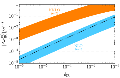
The dependence of these corrections on is plotted in figure 1, where we take between and . The dashed line shows the known exact NLO result for thrust. This implies that when working to NNLO, we need to have a reasonable determination of the NNLO contribution to the cross section. For typical applications with this implies that . To the extent that the NNLO terms are only a small part of the total cross section (as is the case for Drell-Yan, for example), a larger error on the NNLO terms might be tolerable. However, we stress that these estimates can only serve as an indication, and in practice one should carefully test the size of missing corrections, for example by studying the dependence as discussed in section 4.3.
An important comment concerns the fact that it is in principle possible and straightforward (though perhaps tedious in practice) to derive subleading factorization theorems for -jettiness and other observables using SCET. These can then be used to systematically determine the next-to-singular corrections and include them in the same way in the subtractions. This would substantially reduce the size of the missing nonsingular corrections by one power of . A complete factorization theorem at subleading order for a single-jet process has been derived for semileptonic heavy quark decays in ref. Lee:2004ja . For recent work in this direction for thrust in see e.g. refs. Freedman:2013vya ; Freedman:2014uta ; Kolodrubetztalk .
A second important aspect concerns the required numerical precision in a practical implementation. For both -slicing and differential -subtractions, the full QCD and singular cross sections are probed in regions of phase space with , where there are significant numerical enhancements due to the nearby IR singularity at . For , the cancellations between the full QCD and singular distributions can easily reach the level and only increase as is lowered further. Getting a result at relative numerical precision in this case demands at least an relative numerical precision in the evaluation of the squared QCD amplitudes.
For -slicing, the numerical cancellations only happen after the integration, which means that in the worst case the integral itself may have to be carried out to the same high precision. In practice, this will strongly depend on the process and the chosen , since the numerical cancellations actually happen between the two terms in eq. (2.3.1) rather than the the last two terms in eq. (18). In any case, using Monte-Carlo integration to determine the integral of the unsubtracted full result down to very accurately requires very high statistics and good phase-space sampling. Since NLO codes are usually not designed for this purpose, this strongly limits how low can be taken.
For the -subtractions, the QCD amplitudes in the integrand still require the same high numerical precision at small to obtain an accurate result for the nonsingular spectrum. However, since the cancellations now happen already at the integrand level, the integration itself has to be carried out only to the nominal relative precision. Hence, the statistical requirements on the Monte-Carlo integration of the nonsingular spectrum in eq. (2.3.2) are much more modest compared to the -slicing. This also means that can now be taken as low as the numerical precision in the integrand allows. The main nontrivial requirement now is that one must be able to sample phase-space for fixed , which we discuss further in section 4.
3 -jettiness Subtractions
In this section, we now specify to be -jettiness and explicitly construct the -jettiness subtractions. We first discuss the Born kinematics and the definition of -jettiness in section 3.1. In section 3.2 we review the factorization theorem for the singular contributions in and how the virtual QCD amplitudes enter into it. Then in section 3.3 we explicitly write out the subtractions at NLO and NNLO. Finally, in section 3.4 we discuss how the subtractions can be made more differential and thereby more local.
3.1 Definition of -jettiness
3.1.1 Born kinematics
We always use the indices and to label the initial states, and to label the final states. Unless otherwise specified, a generic index always runs over . We denote the momenta of the QCD partons in the Born phase space by and the parton types (including their spin/helicity if needed) by . Thus, corresponds to
| (26) |
where denotes the phase space for any additional nonhadronic particles in the final state, whose total momentum is . (For or collisions, one or both of the incoming momenta are considered part of .) We will mostly suppress the nonhadronic final state. For us, it is only relevant because it contributes to momentum conservation in , which reads
| (27) |
When there is no ambiguity, we will associate (e.g., we use ), and we use the collective label to denote the whole partonic channel, i.e.,
| (28) |
We write the massless Born momenta as
| (29) |
In particular, for the incoming momenta we have
| (30) |
where is the total (hadronic) center-of-mass energy and points along the beam axis. The are the light-cone momentum fractions of the incoming partons, and momentum conservation implies
| (31) |
The total invariant mass-squared and rapidity of the Born phase space are
| (32) |
The complete phase-space measure corresponds to
| (33) |
where on the right-hand side denotes the standard Lorentz-invariant -particle phase space, the sum over runs over all partonic channels, and is the appropriate factor to take care of symmetry, flavor and spin averaging for each partonic channel.
3.1.2 -jettiness
Given an -particle phase space point with , -jettiness is defined as Stewart:2010tn
| (34) |
where runs over . (Here we use a dimension-one definition of following refs. Jouttenus:2011wh ; Jouttenus:2013hs .) For or collisions, one or both of the incoming directions are absent. The are normalization factors, which are explained below. The are the final-state parton momenta (so excluding the nonhadronic final state) of . The in eq. (34) are massless Born “reference momenta”, and the corresponding directions are referred to as the -jettiness axes. For later convenience we also define the normalized vectors
| (35) |
The are obtained by projecting a given onto a corresponding Born point . For this purpose, any IR safe phase-space projection can be used. That is, in any IR singular limit where , the Born projection has to satisfy
| (36) |
including the proper flavor assignments. In particular, for , we simply have and so , which implies . For , there is always at least one that cannot be exactly aligned with any of the , which means that . The minimization condition in eq. (34) ensures that for each the smallest distance to one of the enters the sum, which together with eq. (36) implies that . Hence, -jettiness satisfies all the criteria of an IR-safe -jet resolution variable given in eq. (4).
Some examples of suitable Born projections are discussed in section 3.1.3 below. Although the precise procedure to define the Born projection and the is part of the definition of -jettiness, it is important that it does not actually affect the singular structure of the -differential cross section. Different choices only differ by power-suppressed effects, as explained in ref. Stewart:2010tn , which means the precise choice only affects the nonsingular contributions. Hence, constructing the singular contributions and the subtraction terms does not actually require one to specify the Born projection, as they are constructed in the singular limit starting from a given .888In this regard, the -subtractions are FKS-like, namely they are intrinsically a function of the Born phase space and an emission variable, which for us is , as opposed to starting from a given point. This fact provides considerable freedom in the practical implementation, which we will come back to in section 4.
The singular structure of is determined by the minimization condition in eq. (34) and the choice of the . The minimization effectively divides the phase space into jet regions and up to beam regions, where each parton in is associated (“clustered”) with the it is closest to, where the determine the relative distance measure between the different . We can then rewrite eq. (34) as follows,
| (37) |
where the are the contributions to from the th region.
The can be chosen depending on the Born kinematics in (subject to the constraint that the resulting distance measure remains IR safe). A variety of possible choices are discussed in detail in refs. Jouttenus:2011wh ; Jouttenus:2013hs . An “invariant-mass” measure is obtained by choosing common . In this case, the sum of the invariant masses of all emissions in each region will be minimized. A class of “geometric measures” is obtained by choosing proportional to , which makes the value of itself independent of the , i.e.,
| (38) |
where the are dimensionless numbers which determine the relative size of the different regions. In this case, the sum of the small light-cone momenta, , of all emissions relative to their associated -jettiness axis are minimized.
The singular structure of the cross section does explicitly depend on the distance measure. When discussing the singular contributions in the next section, we will keep the arbitrary, thus enabling various choices to be explored using our results. [As discussed in ref. Stewart:2010tn , one can generalize -jettiness further to use any IR-safe distance measure in eq. (34), which has been used for example in the application to jet substructure Thaler:2010tr ; Thaler:2011gf . For our purposes, the canonical form is suited well, because the simple linear dependence on simplifies the theoretical analysis and computations.]
3.1.3 Example Born projections
To construct a generic Born projection, it suffices to use any IR-safe jet algorithm to cluster the -parton final state into jets with momenta . One can then define massless final-state by taking ()
| (39) |
where any of the choices for can be used. To ensure that the total transverse momentum in the Born final state adds up to zero, one can then for example boost the hadronic system or recoil the leptonic final state in the transverse direction. Finally, the initial-state momenta and , which always lie along the beam directions as in eq. (30), are determined by momentum conservation from eq. (31).
When using a geometric measure as in eq. (38), the canonical way to determine the -jettiness axes is by an overall minimization of the total value of . Up to NNLO the relevant cases are and , i.e., one and two extra emissions, in which case the overall minimization to find the -jettiness axes is still fairly easy to work out explicitly.
Let us take for simplicity and consider the case of hadron-hadron collisions, such that we have jet axes plus the two fixed beam axes . When , it is easy to see that axes must be aligned with of the momenta. For the last axis, there are two possibilities, and the one which gives a smaller is selected: Either it is aligned with one of the two remaining (this occurs if the last momentum lies close enough to one of the beam directions), or it lies along the direction of the sum of the two remaining . The appropriate expression for for is then:
| (40) |
The first term in the overall minimization corresponds to the first case above (extra emission clustered to the beam), whilst the second term corresponds to the second case (extra emission clustered to a jet).
When there are two extra emissions. Now, axes will always be aligned with of the momenta, and there are four possible cases how the remaining two axes can be chosen based on the remaining four . The appropriate expression for for is
| (41) | ||||
The first term in the overall minimization corresponds to both extra particles being clustered to a beam direction. The second term corresponds to one particle being clustered to a beam, and two particles being clustered together in a jet. The third term corresponds to clustering three particles together in a jet, and the final term corresponds to clustering two sets of two particles into two separate jets. In all cases the remaining jet directions are set by the remaining unclustered momenta.
3.2 Factorization in the singular limit
3.2.1 Factorization theorem
We start by writing the -jettiness singular cross section differential in and all individual contributions,
| (42) |
The factorization of the -jettiness cross section in the singular limit [for the linear measures defined by eq. (34)] was derived in SCET in refs. Stewart:2009yx ; Stewart:2010tn ; Jouttenus:2011wh . It takes the form
| (43) | ||||
The first argument(s) of the beam, jet, and soft functions , , and determine the contributions to the from the respective collinear and soft sectors. The beam function contains all collinear emissions (virtual and real) from the incoming parton , and depends on the parton’s flavor and light-cone momentum fraction . The jet function contains all collinear emissions from the outgoing parton , and depends on the parton’s flavor . The soft function contains all soft emissions between all partons and depends on the directions . It is a matrix acting in the color space of the partonic channel . More precisely, it acts in the color-conserving subspace of the full color space. The hard Wilson coefficient is a vector in the same color space, and is its conjugate (see below). It contains the QCD amplitudes for the -parton process and depends on the full -parton phase space .
All functions in the factorized cross sections have an explicit dependence (due to their nonzero anomalous dimensions). This dependence exactly cancels between the different functions at each order. The remaining internal -dependence is the usual one due to the running of which cancels up to the order one is working at. In the general case, the dependence is used to resum the logarithms of to all orders in at a given order in logarithmic counting. For our purposes, we require the strict fixed-order expansion in at NLO and NNLO.
We note in passing that starting at N4LO, the partonic QCD cross section receives a contribution from noncancelling Glauber modes in graphs with the same structure as figure 5 in ref. Gaunt:2014ska . Such contributions are not reproduced by eq. (43). However this is far beyond NNLO, which is the level we are concerned about here.
3.2.2 QCD amplitudes and color space
The hard coefficients contain the virtual -parton amplitudes from QCD. They formally arise as the matching coefficients from QCD onto SCET. How this matching is performed in practice for generic processes using QCD helicity amplitudes is discussed extensively in refs. Stewart:2012yh ; helicityops (see also refs. Kelley:2010fn ; Becher:2013vva ; Moult:2014pja ; Broggio:2014hoa ). We refer the reader there for details and only summarize the features relevant for our discussion here. The important point is that when working in pure dimensional regularization with , the coefficients are given by the infrared-finite part, , of the full -parton QCD amplitude after UV renormalization.999The UV renormalization scheme must be the same for all functions appearing in the factorized cross section. The explicit results we give all use conventional dimensional regularization (CDR), which requires the QCD amplitudes to be renormalized in the CDR or ’t Hooft-Veltman (HV) scheme. Hence, we have
| (44) |
where we have explicitly written out the color indices of the external partons. (All remaining dependence on external helicities and momenta are contained in .)
The color indices span the full color space for the partonic channel . We can now pick a complete basis of color structures , which span the color-conserving subspace. (For practical purposes, the basis can be overcomplete and does not have to be orthogonal.) For example, for the color-conserving subspace is still one-dimensional, since the only allowed color structure is . For , one choice would be
| (45) |
Given a basis , we write the hard coefficients in this basis as
| (46) |
This is in one-to-one correspondence to choosing a particular color decomposition for the -parton amplitude, and so the coefficients are directly given by the IR-finite parts of the color-ordered (or color-stripped) amplitudes. The precise form of the amplitude’s color decomposition is irrelevant for our discussion and any convenient color basis can be used.
The conjugate of the vector is defined by
| (47) |
where the superscript denotes the transpose and
| (48) |
is the matrix of color sums for the basis chosen for the partonic channel . The typically used color bases are not orthonormal, in which case is not equal to the identity operator and is not just the naive complex conjugate transpose of . We then have
| (49) |
3.2.3 Leading order
3.3 Single-differential subtractions
We now project onto the single-differential -jettiness . Equations (3.2.1) and (43) yield
| (53) | ||||
where the single-differential soft function is the projection of the multi-differential one appearing in eq. (43), see eq. (110). We expand this singular contribution to the -jettiness cross section as [cf. eq. (2.2)]
| (54) | ||||
The are the usual plus distributions defined in eq. (2.2). Here we explicitly denote the dependence of the subtraction coefficients on the renormalization scale . The individual coefficients also depend on the arbitrary dimension-one parameter , which drops out exactly in the sum of all coefficients at each order in . (In section 2.2 we used .) Finally, the coefficients also depend on the -jettiness measures , which we suppress for simplicity.
To determine the subtraction coefficients, we simply expand all the functions in the factorization theorem eq. (53) in terms of ,
| (55) |
plug these back, and collect all contributions to each order in and each power in . Explicit results for the jet, beam, and soft functions through are given in Appendix A.
3.3.1 NLO subtractions
At NLO, the differential subtractions require the subtraction coefficients and , which are the coefficients of the and contributions. They are given by (with ),
| (56) |
The jet function contributions in the first line effectively correspond to collinear final-state subtractions, while the beam function contributions in the second line effectively correspond to collinear initial-state subtractions. The soft function contribution in the last line effectively corresponds to a soft subtraction.
As explained in section 2, the coefficient determines the integrated subtractions plus the virtual contributions, which becomes obvious when choosing . At NLO, we have
| (57) |
The first line contains the IR-finite virtual one-loop amplitudes in . The remaining lines effectively correspond to the integrated collinear and soft subtractions. The NLO beam, jet, and soft function coefficients, , , and appearing in eqs. (3.3.1) and (3.3.1) are all known and are collected in Appendix A. The PDF factorization scale () dependence only enters via the beam functions and the PDFs.
One can see that the structure of the subtraction terms has a close resemblance with FKS subtractions. The important difference is that here one does not have to divide up phase space in order to individually isolate all possible IR singular regions. Instead, all the singular regions are projected onto the single variable . An analogous phase-space division for the soft emissions now happens in the calculation of the -jettiness soft function. It is also important to note that there are no overlaps (i.e. double counting) between the soft and collinear subtraction terms. In principle, such overlaps can exist and must be removed, which in SCET corresponds to removing so-called zero-bin contributions Manohar:2006nz . A nice feature of -jettiness is that all such overlap contributions automatically vanish in pure dimensional regularization at all orders in perturbation theory.
3.3.2 NNLO subtractions
For simplicity of the presentation, we define the abbreviations
| (58) |
where we use roman letters (B, J, S, C, f) to avoid any confusion with some of the coefficients listed in Appendix A. The NNLO coefficients and as well as the soft function coefficients are all known analytically, see Appendix A.
The -jettiness soft function describes how the soft radiation is split into the different -jettiness regions. Obtaining the two-loop soft constant (the coefficient of the , see eq. (112)) is the remaining principal challenge. It is known analytically for processes with two external partons, see eqs. (123) and (124), but it is currently unknown for generic -jet processes. It can however be determined numerically by extending the NLO calculation in ref. Jouttenus:2011wh using existing NNLO results. A procedure to do so has been outlined recently in ref. Boughezal:2015eha , where numerical results for -jettiness in collisions were presented.
We conveniently denote the genuine -loop contributions from jet, beam, and soft functions to the as
| (59) |
Using this notation, we write the two-loop cross terms related to real-virtual contributions and involving the one-loop virtual amplitudes in as
| (60) |
Finally, the cross terms with two one-loop coefficients of jet, beam, or soft functions from the associated convolution are denoted as
| (61) |
With these definitions, the NNLO subtraction coefficients read
| (62) | ||||
| (63) | ||||
| (64) | ||||
| (65) | ||||
| (66) | ||||
The coefficient again corresponds to the integrated NNLO subtraction piece and contains the full IR-finite virtual -parton amplitudes in .
The constants multiplying the in equations (62)-(66) are the coefficients arising in the convolution ,
| (67) |
They are given in table 1 for . Their expression for general can be found in Appendix B of ref. Ligeti:2008ac .
3.3.3 Toward N3LO subtractions
Using the notation introduced in the previous subsection it is straightforward to also write down the N3LO -jettiness subtraction terms. Besides the genuine three-loop terms according to eq. (59), we now have “two-loop times one-loop” cross terms and as well as the “(one-loop)3” cross terms , , and , where the latter is associated with the convolution .
The N3LO subtraction coefficients then schematically take the form
| (68) | ||||
The cross terms in eq. (3.3.3) are a linear combination of the above listed ’s, whose numerical coefficients can be easily worked out by evaluating the relevant convolutions among the distributions in analogy to the NNLO case.
For processes with only two colored external partons, so , DIS, or color singlet, analytic expressions for all are in fact available. This is because the three-loop anomalous dimensions of jet and beam functions, the PDFs, and the hard function are known Vogt:2004mw ; Moch:2004pa ; Moch:2005id ; Moch:2005tm ; Becher:2006mr ; Becher:2009th ; Stewart:2010qs ; Berger:2010xi , which also fixes the three-loop soft anomalous dimension. This means the complete set of logarithmic () terms of the renormalized jet, beam, and soft functions are determined by their RGE. The only coefficient that is not fully known is , associated with the integrated N3LO subtractions plus virtual corrections. The are known from the IR-finite parts of the three-loop quark and gluon form factors Baikov:2009bg ; Gehrmann:2010ue . As the cross terms only involve known lower-order contributions, the only missing piece in eq. (3.3.3) then is , for which one has to compute the three-loop -independent constants of the jet, beam, and soft functions.
3.4 Constructing more-differential subtractions
As mentioned already, the -subtractions we have defined thus far are nonlocal, in the sense that all the singular regions are projected onto the single variable and the subtraction acts only after the corresponding phase-space integrations. It is conceivable that in order to improve the numerical stability or convergence of the NNLO calculation one might wish to use a more local subtraction – indeed, many of the available NNLO subtraction schemes utilize highly local subtraction terms.
In our approach, it is straightforward, at least conceptually, to progressively increase the locality of the subtractions. All one needs to do is split up into further IR-safe observables that cover the phase space and which are sensitive to emissions in different regions, and/or introduce further observables that resolve the nature of emissions, e.g. allowing one to discriminate between double-real and single-real(+virtual) emissions in a given region. The subtraction is then given by the singular cross section differential in all of these observables. In practice, this requires the relevant factorization theorem for this more-differential cross section.
Let us demonstrate how this works for a simple example. The factorization theorem in eq. (43) is already differential in the individual -jettiness contributions . For simplicity, we take and consider the NNLO cross section. In this case, -jettiness (aka beam thrust) effectively splits the event into two hemispheres (beam regions) and , whose -jettiness axes are defined by the beam directions. The total -jettiness is given by , where and are the contributions from the two hemispheres [cf. eq. (37) and its discussion].
Following the procedure in section 3.3 we can use the total to construct a subtraction. However, instead of taking the sum, we can also consider and separately, and perform the subtraction differential in both of these observables. Each of them is then sensitive to a subset of the singular regions, namely, collinear (and soft) emissions closer to beam will only affect , whilst emissions closer to beam will only affect .
Following the logic of section 2.3, we first write down the appropriate formula for the corresponding double-differential phase-space slicing:
| (69) |
Here, we substitute in the double-differential singular cross section when both and are below the IR cutoff , which is correct up to . Having either or nonzero requires at least one additional emission, so the remaining three regions only require an NLO calculation. Of course, there are singularities in the second term as with nonzero (and similar singularities in the third term when with nonzero ), but these are handled as part of the NLO calculation.
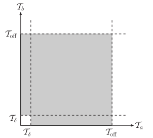
Performing the slicing method using both and has no clear advantage over the slicing method using alone, as in both methods one basically removes a small region of size around , and handles it using the singular cross section. However, let us rewrite eq. (3.4) as a subtraction by adding and subtracting the singular cross section for the shaded region in figure 2, arranged in the following way:
| (70) |
This equation is the two-variable analogue of eq. (2.3.2). The parameter controls again where we turn off the subtraction, and the dependence on it precisely cancels between all contributions. The total cumulant in the first term contains the two-loop virtual corrections together with the corresponding integrated subtraction terms. The cross sections in the second and third terms are differential in one of the variables and integrated in the other. Since one of the variables is nonzero, while the other is integrated, they require an NLO calculation with one additional resolved emission. These terms contain all the real-virtual contributions and the singular cross section acts as the corresponding real-virtual subtraction. The fourth term involves the double-differential cross sections and since both variables are nonzero only requires a LO calculation with two resolved emissions, one in each hemisphere. The double-differential singular cross section then acts as the corresponding double-real subtraction, which is point-by-point in both and . (Contributions with two real emissions in the same hemisphere are part of the NLO calculations in the second and third terms.) Hence, by considering separately and , one is able to disentangle different real-virtual and double-real contributions and also make the subtractions more local. The price one has to pay is that the double-differential singular cross section in the last term requires the double-differential NNLO soft function, which is more complicated. (For the beam and jet functions this requires no additional effort.)
A further important point to make is that and are defined such that requiring or forces the corresponding emission to be in hemisphere or . At NLO, there is only one real emission, so only one out of and can be nonzero. Then, the double-differential subtraction essentially splits the -subtraction into two pieces, acting in the two hemispheres. At NNLO, this splits the real-virtual contributions into the two pieces in the second and third lines of eq. (3.4). If this is undesired, one can instead consider the two variables and . This effectively folds the phase space in figure 2 in half along the diagonal where , and combines the second and third terms in eq. (3.4) into one.
Now let us return to the general case with partons in the Born process. Then there are contributions , and one can consider the subtraction separately in all of them. At NLO, only one of them can be nonzero, while at NNLO at most two of them can be nonzero. This means that there will be many different contributions, where in each contribution only one or two of the are differential and nonzero, while all the others are integrated over. Each can only be nonzero when the corresponding emission is in the th -jettiness region. Hence, if desired, using the individual as the resolution variables automatically yields a division of phase space into different singular regions around each of the partons, very similar to the phase-space divisions encountered in traditional local subtraction methods. On the other hand, if the proliferation of phase-space regions is undesired, one can still have the same gain at NNLO as in eq. (3.4) by considering two combinations of all , e.g. the minimum and maximum nonzero , or the sum of all together with the sum of all but the largest .
Instead of or in addition to splitting into its different components, one can also increase the locality of the subtraction by performing it differentially in both and another independent -jet resolution variable. For example, one could look into each -jettiness region and compute the scalar sum of transverse momenta with respect to the corresponding -jettiness axis , performing the subtraction also differential in the . Doing so resolves part of the radiation phase space, which would otherwise be integrated over when considering only by itself. For the case one could for example consider together with the transverse momentum of the color-singlet final state . The relevant factorization formulae differential in and have been discussed and written down in refs. Jain:2011iu ; Procura:2014cba (see also refs. Collins:2007ph ; Rogers:2008jk ), and the corresponding double-differential two-loop quark beam functions have been computed in ref. Gaunt:2014xxa .
We have discussed several options how to extend the single-differential -jettiness subtractions, but of course this is not an exhaustive list. Constructing such more-differential subtractions requires the appropriate singular cross section differential in all of the chosen jet resolution variables, and in order to experience the maximum advantage in terms of convergence, these differential cross sections should reproduce the correct singular behaviour in all of the relevant singular kinematic regimes. The factorization of multi-differential cross sections in SCET accurate in all relevant kinematic regimes is a topic that has received much interest recently, see e.g. refs. Bauer:2011uc ; Jouttenus:2011wh ; Jouttenus:2013hs ; Procura:2014cba ; Larkoski:2014tva ; Larkoski:2015zka , and it would be interesting to apply this work to the issue of calculating NNLO QCD cross sections.
4 Practical Considerations and Implementation
In this section, we discuss in more detail how the singular cross section in eq. (54) can be implemented in practice as a subtraction term following our general discussion in section 2.3. We first discuss the NLO case in section 4.1, where we also highlight the similarities to FKS subtractions, and then the NNLO case in section 4.2. In section 4.3, we discuss numerical aspects using the NNLO rapidity spectrum in Drell-Yan and gluon-fusion Higgs production as an example.
4.1 NLO
4.1.1 FKS subtractions
In the notation of eq. (1), the cross section at NLO is given by
| (71) |
where is the -parton virtual one-loop contribution and is the -parton real-emission contribution,
| (72) |
The additional in compared to is contained in . As indicated in eq. (4.1.1), the limit can only be taken in the sum of and integral over .
When implementing eq. (4.1.1) using FKS subtractions Mangano:1991jk ; Frixione:1995ms ; Frixione:1997np ; Frederix:2009yq ; Alioli:2010xd , the cross section is obtained as follows:
| (73) |
Here, the phase space is first sampled over . For a fixed point, one then further samples over the radiation phase space , where the sum over runs over all the different IR-singular regions. The real-emission contribution and measurement are evaluated at a constructed point . The superscript on indicates that is divided up between the regions in such a way that it is precisely reproduced in the sum over all regions. The phase-space map and the subtraction terms are specific to each singular region. The are directly constructed in the singular limit, meaning they are functions of and only, and in particular do not depend on the actual map . In practice, there is again a tiny IR cutoff required on the integral due to limited numerical precision and the fact that and each individually diverge. The subtracted virtual, , contains the finite remainder after combining the virtual contributions with the integral of the subtractions and cancelling all IR poles.
4.1.2 -subtractions
As discussed in section 2.3, the full cross section for at only requires a lower-order calculation. At NLO, we need its LO expression given by
| (74) |
where it is obvious that this is a LO quantity.
Since the subtractions are used up to the upper cutoff , as seen in eq. (2.3.2), it is most convenient to set in the subtraction coefficients. For the singular spectrum at , we can simply drop and replace . The subtraction terms at NLO are then
| (75) |
where for convenience we included the in the singular spectrum.
Using the above with eq. (2.3.1), the -slicing at NLO becomes
| (76) |
This calculation is very easy from an implementation point of view, since it boils down to performing two LO phase-space integrals. As already eluded to, the main practical limitation are the large numerical cancellations between both terms, requiring the phase-space integrals to be evaluated to very high precision.
Using eq. (74), the differential -subtraction in eq. (2.3.2) takes the form
| (77) |
For a numerical implementation, one must be able to solve the function in the integral, which amounts to being able to sample over all of that gives a fixed . One option to do so is to decompose as
| (78) |
where is precisely the Born projection used to define , see section 3.1. The contains the remaining information needed to fully specify , which includes the continuous angular radiation variables as well as the discrete information about flavor, spin, and in which -jettiness region the additional emission goes. We can then rewrite eq. (4.1.2) as
| (79) | ||||
One now samples first over and then . For fixed and , one further samples over and evaluates the real-emission contribution at the point reconstructed from all of these. Being able to reconstruct is equivalent to inverting the Born projection. Recall however, that the singular contributions are independent of the Born projection. Therefore, one has the freedom to specifically choose the Born projection to facilitate this inversion, making it easily possible.
Note that the integral contains a discrete sum over all -jettiness axis/regions. If one were to separate into its individual components as discussed in section 3.4, this sum would become explicit and the single subtraction term would effectively separate into different subtraction terms for each region.
4.2 NNLO
At NNLO, the subtraction terms are
| (80) |
As at NLO, we have chosen and included the in the singular spectrum.
The full -differential cross section at is now needed at NLO, where it is given by
| (81) |
In the second equation we wrote it in the form of an NLO calculation with FKS-like subtractions, analogous to eq. (4.1.1), where now .
In general, the map used in the -jet NLO calculation will not preserve , that is, . This means we have to be careful in implementing the cutoff, because in order for the neglected pieces to be nonsingular, the cutoff must be applied on the true . We can do this by treating the cutoff analogous to the measurement . That is, we define the NLO calculation
| (82) |
which is fully-differential in and satisfies
| (83) |
Using the above together with eq. (2.3.1), the -slicing at NNLO is given by
| (84) |
This is again quite easy to implement, only requiring a LO phase-space integral for the first term and a NLO calculation for the second term. The practical limitation is the achievable numerical precision in the NLO calculation and the integral, which strongly limits how low can be pushed.
From eq. (2.3.2), the differential -subtraction at NNLO takes the form
| (85) |
To implement this numerically, one must be able to compute the spectrum to NLO for a given , which requires to solve the functions in eq. (4.2). For we can use the same procedure as at NLO together with the -jet NLO cross section , giving
| (86) |
This can be implemented like the NLO case in eq. (79), with the LO replaced by . The subtraction in eq. (4.2) is not completely local in , since the points being integrated over in will generically not have the correct value. However, a simple phase-space map that approximately preserves might be sufficient in practice.
To achieve an exact point-by-point cancellation in , one also has to solve the constraint in eq. (4.2). This requires constructing a map for the -jet NLO calculation that preserves so and is equivalent to inverting the Born projection underlying the definition of . This is quite a bit more challenging than at NLO. It has been achieved in ref. Alioli:2012fc for a slightly modified version of . Assuming, we have a map like this, we can pull the cut out of the NLO calculation, such that
| (87) | ||||
The differential -subtraction then becomes
| (88) |
The subtraction is now fully localized in , and the only nonlocality is in the variables.
In a practical implementation of eq. (4.2) or eq. (4.2), the subtraction terms are easily evaluated and the most nontrivial ingredient is in fact the NLO calculation of , for which one can use any existing FKS-like NLO calculation or one can iterate the -jettiness subtractions and perform it using -subtractions. Note that in all cases above the measurement is performed inside . If the map preserves , so , then it can be pulled out of the -jet NLO calculation.
4.3 Example: NNLO rapidity spectrum for Drell-Yan and Higgs
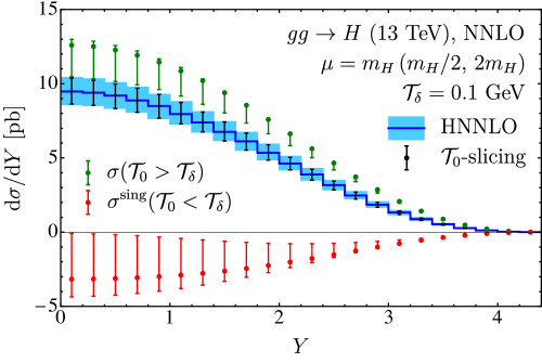
To illustrate our method with a nontrivial example, we consider the rapidity distribution of the vector boson in Drell-Yan production, , and of the Higgs boson in gluon fusion, , which are known to NNLO Anastasiou:2003yy ; Anastasiou:2003ds ; Anastasiou:2004xq ; Anastasiou:2005qj ; Catani:2007vq ; Grazzini:2008tf ; Catani:2009sm . Since the size of the perturbative corrections in the two cases are very different, they provide very useful and complementary test cases.
In both cases, 0-jettiness is the resolution variable and all of the ingredients necessary to implement the -subtractions through NNLO are known. (We use the geometric measure with , see eq. (38), which makes identical to beam thrust.) The results are obtained for the LHC with a center-of-mass energy of . We always use CT10 NNLO PDFs Gao:2013xoa . We choose common renormalization and factorization scales, , with for Drell-Yan production and for Higgs production. For the latter we use and work in the top EFT limit. For the -jet and -jet NLO calculations we use MCFM Campbell:2002tg ; Campbell:2010ff .
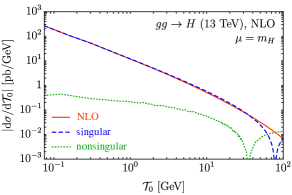
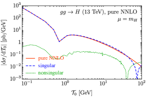
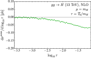
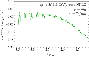
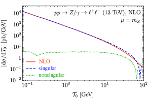
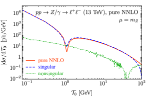
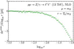
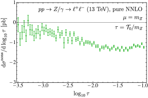
An important validation of the -jettiness subtractions is to confirm that the singular spectrum is correctly describing the singularities of the full QCD result. This is done by calculating the nonsingular spectrum as in eq. (2.2) as the difference of the full QCD and singular spectra. The decomposition of the spectrum into singular and nonsingular components is shown in figures 3 and 5 for Drell-Yan and Higgs production, respectively, where we separately show the (NLO) and (pure NNLO) corrections, counted relative to the LO Born cross section. (We plot the magnitudes of the contributions on a logarithmic scale, and the dips at large and around are due to the spectra going through 0. The small jitters in the pure NNLO nonsingular are due to numerical inaccuracies.) One can clearly see the large numerical cancellations between the full and singular results for small , where the nonsingular spectrum is several orders of magnitude smaller than the full and singular spectra.
As shown in eq. (2.3.2), the nonsingular spectrum is precisely the quantity that one integrates numerically when using the differential -subtractions. The fact that the nonsingular only contains integrable singularities is seen in figures 3 and 5 by its smaller slope toward . To check explicitly that the subtractions work and the nonsingular does not contain any singularities, we consider the distribution , which must go to 0 in the limit. We plot it in figure 4 for Drell-Yan and in figure 6 for Higgs production, again separately for the NLO and pure NNLO corrections, and using and , respectively. One can see that for , as it must. The error bars come from the statistical integration uncertainties in the full result obtained from MCFM. The numerical uncertainties in the singular result are negligible in comparison.
To obtain results for the NNLO rapidity spectrum, we use the simple -slicing in eq. (84). As explained earlier, the missing contributions due to the cutoff are the same irrespective of how the subtractions are implemented. At NLO, we use ( for Drell-Yan and for Higgs) and at NNLO we use ( for Drell-Yan and for Higgs). These values are at the lower end of values plotted in figures 4 and 6, and are mainly limited by the MCFM statistics.
Specifically, we use MCFM to compute the NLO cross section for in the second term in eq. (84),
| (89) |
in bins of for the processes and . Since there are no cuts on the final-state jets other than the requirement , for small the calculation probes deep into the singular region and care must be taken to obtain reliable and numerically stable results. This is combined with our own implementation of the NNLO singular cross section for , , in the first term of eq. (84).
The results for the rapidity spectra are shown in figures 7 and 9 for Drell-Yan and Higgs production, respectively. The two contributions from and are shown in red and green and the total result given by their sum in black. The error bars here show the scale variations up and down by a factor of two. Note that the relative size of the two contributions and the degree of cancellation between them can change significantly as the scale (or value) is changed. To validate the results from -slicing method, we compare to results from Vrap Anastasiou:2003yy ; Anastasiou:2003ds for Drell-Yan and from HNNLO Catani:2007vq ; Grazzini:2008tf for Higgs, which are shown by the blue line and band. For both processes we find excellent agreement.
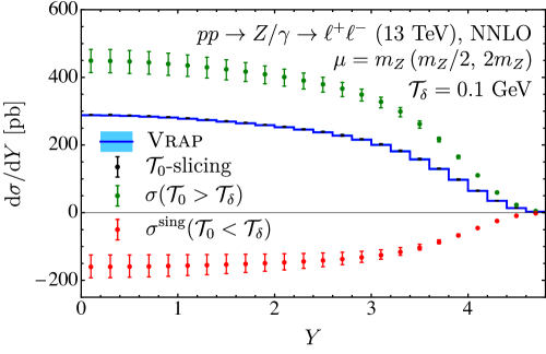
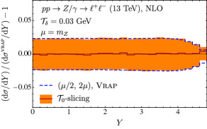
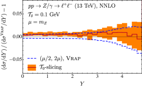
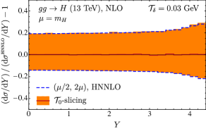
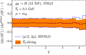
In figures 8 and 10 we show the fractional difference of the -slicing results relative to Vrap and HNNLO, respectively. At NLO with , the agreement is excellent. For Drell-Yan at NNLO, there is a small offset between the two results visible in figure 8, representing of the total cross section. A similar offset of is also present in the Higgs case, but hardly visible because the scale variations are much larger. It is due to the missing nonsingular terms for . A smaller value of would be needed to reduce this effect. The size of the missing nonsingular terms we observe here is consistent with their expected size from our estimates in section 2.3.3. Nevertheless, it is actually encouraging to see that even with the simple -slicing we are able to obtain this level of agreement. We would expect that an implementation of the differential -subtractions will allow one to use values well below .
We conclude this discussion by noting that it is important, particularly for more complex processes, to carefully quantify the size of the neglected nonsingular contributions. In particular, as already seen in figure 1, one cannot draw any conclusions for their possible size at NNLO from knowing their size at NLO. Also, the difference in the result when varying the value is not necessarily a good estimate of the absolute size of the missing nonsingular terms, because as discussed in section 2.3.3, their scaling with for is much weaker than linear. A crucial check one should perform is to plot the nonsingular distribution as in figures 4 and 6 and check its convergence toward zero.
5 Conclusions
Higher-order computations in QCD require the use of some subtraction technique that allows one to extract the collinear and soft phase-space divergences from the real-emission diagrams, and cancel these against the explicit divergences from the virtual loop diagrams. We explained how a subtraction scheme can be constructed using an IR safe -jet resolution variable to control the approach to the IR-singular limit. The -jettiness observable is ideally suited for this task due to its known and simple factorization properties. Our resulting -jettiness subtraction method is similar in spirit to the subtraction method introduced by Catani and Grazzini for color-singlet production, but may be applied to processes with arbitrarily many colored final-state partons (plus any color-singlet final state).
In our method, the subtraction term corresponds to the appropriate fixed-order expansion of the singular -jettiness cross section, which can be efficiently computed using SCET. In this context, SCET allows the subtraction term to be broken down into various pieces (beam, jet, and soft functions) that are easier to compute, with the beam and jet functions being reusable for processes with any number of jets. The extension to N3LO is possible and requires the calculation of the beam, jet, and soft functions at three-loop order.
We discussed in depth the details of the subtraction procedure, giving explicitly the equations and ingredients needed to construct the -subtraction terms at NLO and NNLO. The only ingredient which is not explicitly known is the -independent constant term of the NNLO -jet soft function for three or more -jettiness axes. It can however be obtained relatively straightforward with existing technology. We also discussed how the -jettiness subtractions can be implemented in practice. To demonstrate the method and study some of its numerical aspects, we presented NNLO results for the Drell-Yan and Higgs rapidity spectra computed using -jettiness subtractions in its simplest form as a slicing method. The slicing method has been previously shown to be successful for NNLO computations in ref. Gao:2012ja and very recently in refs. Boughezal:2015dva ; Boughezal:2015aha . Given the viability of the -slicing, it will be very interesting to extend the implementations to the differential -jettiness subtractions.
We have also suggested and discussed several different ways in which the numerical convergence of the -jettiness subtraction method can be systematically improved. One option would be to include the leading nonsingular terms in the subtraction. These corrections are described by subleading factorization theorems for -jettiness and SCET offers a systematic framework to compute them. Another way to improve the numerical convergence would be to make the subtraction more local, by performing the subtraction differentially in additional observables (such as ) and/or splitting the total -jettiness observable into its components in the jet and beam regions. Much of the recent work in SCET on deriving factorization formulae for multi-differential cross sections can be very useful in this direction.
We only explicitly discussed the case of massless partons here. The construction of analogous -subtractions for processes involving massive quarks is possible with the same techniques. For , one would consider a massive quark jet with its own -jettiness axis making use of the tools in SCET developed for the treatment of massive collinear quarks Leibovich:2003jd ; Fleming:2007qr ; Fleming:2007xt ; Jain:2008gb ; Gritschacher:2013tza ; Pietrulewicz:2014qza . For , e.g. pair production and similar processes, an analogous approach to refs. Zhu:2012ts ; Catani:2014qha can be used. This amounts to treating the heavy quarks as part of the hard interaction (without its own -jettiness axis) together with a more complicated soft function to account for soft gluon emissions from the heavy quarks. We leave further development in this direction to future work.
Acknowledgements.
We thank Kirill Melnikov, Iain Stewart, and Fabrizio Caola for discussions and comments on the manuscript. JRG and MS thank the theory group at LBL for hospitality during part of this work. This work was supported by the DFG Emmy-Noether Grant No. TA 867/1-1 and by the Office of Science, Office of High Energy Physics, of the U.S. Department of Energy (DOE) under Contract No. DE-AC02-05CH11231. This research used resources of the National Energy Research Scientific Computing Center, which is supported by the Office of Science of the DOE under Contract No. DE-AC02-05CH11231.Appendix A Subtraction Ingredients
We write the expansion of the QCD beta function and the cusp and noncusp anomalous dimensions as
| (90) |
and
| (91) |
The coefficients of the beta function and cusp anomalous dimensions we need are
| (92) |
and
| (93) |
For the quark jet and beam functions in we have Becher:2006mr ; Stewart:2010qs
| (94) |
For the gluon jet and beam functions in we have Fleming:2003gt ; Becher:2009th ; Berger:2010xi
| (95) |
A.1 Jet function
We write the expansion of the quark () and gluon () jet functions as
| (96) |
The coefficients have the form
| (97) |
where the are plus distributions as defined in eq. (2.2). The jet function is naturally a distribution in , and this is the only dependence of the coefficients. Rescaling the arguments of the distributions using eq. (13), we have
| (98) |
where is an arbitrary dimension-one parameter, which exactly cancels between the different rescaled coefficients and that we can choose at our convenience. The are the coefficients appearing in the explicit expressions for the subtraction terms in sections 3.3.1 and 3.3.2.
The jet function coefficients in eq. (97) read up to two loops
| (99) |
The pieces for the quark jet function are Bauer:2003pi ; Becher:2006qw
| (100) |
and for the gluon jet function they are Fleming:2003gt ; Becher:2009th ; Becher:2010pd
| (101) | ||||
A.2 Beam function
The beam function is given by Stewart:2009yx ; Stewart:2010qs
| (102) |
where are the standard PDFs and are perturbative matching coefficients. Here, we have explicitly separated the dependence, which cancels between the matching coefficients and the PDFs, such that the beam function is independent up to higher orders in . (Usually, one takes in the fixed-order beam function, since these are not really formally distinct scales.) For our purposes, the dependence in the beam function determines the complete factorization scale dependence in the singular fixed-order cross section, while the dependence contributes to the usual renormalization scale dependence.
We expand the beam function matching coefficients as
| (103) |
The perturbative coefficients have the structure
| (104) |
where the are the plus distributions defined in eq. (2.2). The beam function is naturally a distribution in . Rescaling the arguments of the distributions using eq. (13), we have
| (105) |
where is an arbitrary dimension-one parameter, which exactly cancels between the different rescaled coefficients and that we can choose at our convenience. From these coefficients we also define the corresponding beam function coefficients as
| (106) |
which are the coefficients appearing in the explicit expressions for the subtraction terms in sections 3.3.1 and 3.3.2.
The results for the coefficients in eq. (104) are as follows. At LO, we simply have
| (107) |
The NLO coefficients have been computed in refs. Stewart:2009yx ; Stewart:2010qs ; Berger:2010xi , and are given by
| (108) |
The NNLO coefficients have been computed in refs. Gaunt:2014xga ; Gaunt:2014cfa , and read
| (109) |
Explicit results for the matching functions and as well as the splitting functions and and all required convolutions between them can be found in refs. Gaunt:2014xga ; Gaunt:2014cfa in the same notation that we use here.
A.3 Single-differential soft function
The single-differential -jettiness soft function is related to the one of eq. (43), which is multi-differential in the soft contributions to the , by
| (110) |
Recall that the subscript encodes the information on the Born partonic channel. For the soft function, it specifies the color space of the external partons in which it acts.
We expand the soft function in as
| (111) |
where the perturbative coefficients can be written as
| (112) |
The soft function is naturally a distribution in and this is the only dependence of the coefficients. Rescaling the arguments of the plus distributions using eq. (13), we have
| (113) |
The dimension-one parameter is again arbitrary and exactly cancels between the coefficients. The coefficients are those appearing in the explicit expressions for the subtraction terms in sections 3.3.1 and 3.3.2. In the rest of this subsection the dependence on the jet axes of the soft function and its anomalous dimension is always understood and we often suppress the explicit argument.
The renormalization scale dependence of the soft function is subject to the renormalization group equation derived in ref. Jouttenus:2011wh ,
| (114) |
with the soft anomalous dimension
| (115) |
Here, if the partons and are both incoming or both outgoing and if one of them is incoming and the other one outgoing. The invariant
| (116) |
is always positive with our conventions and corresponds to an angular measure between any two partons (depending on the precise choice of the ). Note that here has the overall color factor removed, see eqs. (91) and (A). To write the last line in eq. (A.3), we defined the abbreviations
| (117) |
Note that for and collisions, is always proportional to and can be ignored, as it drops out of eq. (114). Similarly, for collisions it can be ignored for -jet and -jet processes where the color space is still trivial. Up to two loops the noncusp soft anomalous dimension is given by
| (118) |
The fixed-order coefficients in eq. (112) are as follows. At leading order, we have
| (119) |
The one-loop coefficients are given by Jouttenus:2011wh
| (120) |
where
| (121) |
The and are finite phase-space integrals, which are required for three or more -jettiness axes. They are not known fully analytically, but can be evaluated numerically for a given set . Their explicit expressions and an algorithm to reduce them to simple one-dimensional numerical integrals for arbitrary is provided in ref. Jouttenus:2011wh . With only three -jettiness axes, the integrals are still planar. Starting from four axes, the angles also enter, which are the azimuthal angles between the and axes in the plane transverse to the and axes.
Iteratively solving the RGE in eq. (114), we obtain the two-loop coefficients
| (122) |
For two external partons, and , the result for the two-loop constant is known analytically Kelley:2011ng ; Monni:2011gb ; Hornig:2011iu and does not depend on the whether the partons are incoming or outgoing, i.e., it is the same for , , and , and similarly for two gluons Kang:2015moa ,
| (123) | ||||
| (124) |
The two-loop constants () required e.g. for -jettiness in collisions, have recently been computed numerically in ref. Boughezal:2015eha . The two-loop constant for arbitrary -jet processes can in principle be obtained numerically from known results for two-loop soft amplitudes as outlined in ref. Boughezal:2015eha .
References
- (1) M. L. Mangano, P. Nason, and G. Ridolfi, Heavy quark correlations in hadron collisions at next-to-leading order, Nucl. Phys. B373 (1992) 295–345.
- (2) S. Frixione, Z. Kunszt, and A. Signer, Three jet cross-sections to next-to-leading order, Nucl. Phys. B467 (1996) 399–442, [hep-ph/9512328].
- (3) S. Frixione, A General approach to jet cross-sections in QCD, Nucl. Phys. B507 (1997) 295–314, [hep-ph/9706545].
- (4) S. Catani and M. H. Seymour, The Dipole formalism for the calculation of QCD jet cross-sections at next-to-leading order, Phys. Lett. B 378 (1996) 287–301, [hep-ph/9602277].
- (5) S. Catani and M. H. Seymour, A General algorithm for calculating jet cross-sections in NLO QCD, Nucl. Phys. B485 (1997) 291–419, [hep-ph/9605323].
- (6) S. Catani, S. Dittmaier, M. H. Seymour, and Z. Trocsanyi, The Dipole formalism for next-to-leading order QCD calculations with massive partons, Nucl. Phys. B627 (2002) 189–265, [hep-ph/0201036].
- (7) S. Weinzierl, Subtraction terms at NNLO, JHEP 0303 (2003) 062, [hep-ph/0302180].
- (8) S. Frixione and M. Grazzini, Subtraction at NNLO, JHEP 0506 (2005) 010, [hep-ph/0411399].
- (9) G. Somogyi, Z. Trocsanyi, and V. Del Duca, Matching of singly- and doubly-unresolved limits of tree-level QCD squared matrix elements, JHEP 0506 (2005) 024, [hep-ph/0502226].
- (10) G. Somogyi, Z. Trocsanyi, and V. Del Duca, A Subtraction scheme for computing QCD jet cross sections at NNLO: Regularization of doubly-real emissions, JHEP 0701 (2007) 070, [hep-ph/0609042].
- (11) G. Somogyi and Z. Trocsanyi, A Subtraction scheme for computing QCD jet cross sections at NNLO: Regularization of real-virtual emission, JHEP 0701 (2007) 052, [hep-ph/0609043].
- (12) G. Somogyi and Z. Trocsanyi, A Subtraction scheme for computing QCD jet cross sections at NNLO: Integrating the subtraction terms. I., JHEP 0808 (2008) 042, [arXiv:0807.0509].
- (13) U. Aglietti, V. Del Duca, C. Duhr, G. Somogyi, and Z. Trocsanyi, Analytic integration of real-virtual counterterms in NNLO jet cross sections. I., JHEP 0809 (2008) 107, [arXiv:0807.0514].
- (14) P. Bolzoni, S.-O. Moch, G. Somogyi, and Z. Trocsanyi, Analytic integration of real-virtual counterterms in NNLO jet cross sections. II., JHEP 0908 (2009) 079, [arXiv:0905.4390].
- (15) P. Bolzoni, G. Somogyi, and Z. Trocsanyi, A subtraction scheme for computing QCD jet cross sections at NNLO: integrating the iterated singly-unresolved subtraction terms, JHEP 1101 (2011) 059, [arXiv:1011.1909].
- (16) V. Del Duca, G. Somogyi, and Z. Trocsanyi, Integration of collinear-type doubly unresolved counterterms in NNLO jet cross sections, JHEP 1306 (2013) 079, [arXiv:1301.3504].
- (17) G. Somogyi, A subtraction scheme for computing QCD jet cross sections at NNLO: integrating the doubly unresolved subtraction terms, JHEP 1304 (2013) 010, [arXiv:1301.3919].
- (18) V. Del Duca, C. Duhr, G. Somogyi, F. Tramontano, and Z. Trócsányi, Higgs boson decay into b-quarks at NNLO accuracy, JHEP 1504 (2015) 036, [arXiv:1501.07226].
- (19) A. Gehrmann-De Ridder, T. Gehrmann, and E. N. Glover, Infrared structure of jets at NNLO, Nucl. Phys. B691 (2004) 195–222, [hep-ph/0403057].
- (20) A. Gehrmann-De Ridder, T. Gehrmann, and E. N. Glover, Antenna subtraction at NNLO, JHEP 0509 (2005) 056, [hep-ph/0505111].
- (21) A. Daleo, T. Gehrmann, and D. Maitre, Antenna subtraction with hadronic initial states, JHEP 0704 (2007) 016, [hep-ph/0612257].
- (22) A. Daleo, A. Gehrmann-De Ridder, T. Gehrmann, and G. Luisoni, Antenna subtraction at NNLO with hadronic initial states: initial-final configurations, JHEP 1001 (2010) 118, [arXiv:0912.0374].
- (23) E. Nigel Glover and J. Pires, Antenna subtraction for gluon scattering at NNLO, JHEP 1006 (2010) 096, [arXiv:1003.2824].
- (24) R. Boughezal, A. Gehrmann-De Ridder, and M. Ritzmann, Antenna subtraction at NNLO with hadronic initial states: double real radiation for initial-initial configurations with two quark flavours, JHEP 1102 (2011) 098, [arXiv:1011.6631].
- (25) T. Gehrmann and P. F. Monni, Antenna subtraction at NNLO with hadronic initial states: real-virtual initial-initial configurations, JHEP 1112 (2011) 049, [arXiv:1107.4037].
- (26) A. Gehrmann-De Ridder, T. Gehrmann, and M. Ritzmann, Antenna subtraction at NNLO with hadronic initial states: double real initial-initial configurations, JHEP 1210 (2012) 047, [arXiv:1207.5779].
- (27) J. Currie, E. Glover, and S. Wells, Infrared Structure at NNLO Using Antenna Subtraction, JHEP 1304 (2013) 066, [arXiv:1301.4693].
- (28) J. Currie, A. Gehrmann-De Ridder, E. Glover, and J. Pires, NNLO QCD corrections to jet production at hadron colliders from gluon scattering, JHEP 1401 (2014) 110, [arXiv:1310.3993].
- (29) C. Anastasiou, K. Melnikov, and F. Petriello, A new method for real radiation at NNLO, Phys. Rev. D 69 (2004) 076010, [hep-ph/0311311].
- (30) T. Binoth and G. Heinrich, Numerical evaluation of phase space integrals by sector decomposition, Nucl. Phys. B693 (2004) 134–148, [hep-ph/0402265].
- (31) M. Czakon, A novel subtraction scheme for double-real radiation at NNLO, Phys. Lett. B693 (2010) 259–268, [arXiv:1005.0274].
- (32) M. Czakon, Double-real radiation in hadronic top quark pair production as a proof of a certain concept, Nucl. Phys. B849 (2011) 250–295, [arXiv:1101.0642].
- (33) R. Boughezal, K. Melnikov, and F. Petriello, A subtraction scheme for NNLO computations, Phys. Rev. D 85 (2012) 034025, [arXiv:1111.7041].
- (34) M. Brucherseifer, F. Caola, and K. Melnikov, corrections to fully-differential top quark decays, JHEP 1304 (2013) 059, [arXiv:1301.7133].
- (35) R. Boughezal, F. Caola, K. Melnikov, F. Petriello, and M. Schulze, Higgs boson production in association with a jet at next-to-next-to-leading order in perturbative QCD, JHEP 1306 (2013) 072, [arXiv:1302.6216].
- (36) M. Czakon, P. Fiedler, and A. Mitov, Total Top-Quark Pair-Production Cross Section at Hadron Colliders Through , Phys. Rev. Lett. 110 (2013) 252004, [arXiv:1303.6254].
- (37) M. Czakon and D. Heymes, Four-dimensional formulation of the sector-improved residue subtraction scheme, Nucl. Phys. B890 (2014) 152–227, [arXiv:1408.2500].
- (38) R. Boughezal, F. Caola, K. Melnikov, F. Petriello, and M. Schulze, Higgs boson production in association with a jet at next-to-next-to-leading order, arXiv:1504.07922.
- (39) S. Catani and M. Grazzini, An NNLO subtraction formalism in hadron collisions and its application to Higgs boson production at the LHC, Phys. Rev. Lett. 98 (2007) 222002, [hep-ph/0703012].
- (40) S. Catani, L. Cieri, G. Ferrera, D. de Florian, and M. Grazzini, Vector boson production at hadron colliders: a fully exclusive QCD calculation at NNLO, Phys. Rev. Lett. 103 (2009) 082001, [arXiv:0903.2120].
- (41) S. Catani, L. Cieri, D. de Florian, G. Ferrera, and M. Grazzini, Diphoton production at hadron colliders: a fully-differential QCD calculation at NNLO, Phys. Rev. Lett. 108 (2012) 072001, [arXiv:1110.2375].
- (42) G. Ferrera, M. Grazzini, and F. Tramontano, Associated WH production at hadron colliders: a fully exclusive QCD calculation at NNLO, Phys. Rev. Lett. 107 (2011) 152003, [arXiv:1107.1164].
- (43) G. Ferrera, M. Grazzini, and F. Tramontano, Associated production at hadron colliders: the fully differential NNLO QCD calculation, Phys. Lett. B 740 (2015) 51–55, [arXiv:1407.4747].
- (44) Cascioli, F. and Gehrmann, T. and Grazzini, M. and Kallweit, S. and Maierhöfer, P. and others, ZZ production at hadron colliders in NNLO QCD, Phys. Lett. B 735 (2014) 311–313, [arXiv:1405.2219].
- (45) T. Gehrmann, M. Grazzini, S. Kallweit, P. Maierhöfer, A. von Manteuffel, et. al., Production at Hadron Colliders in Next to Next to Leading Order QCD, Phys. Rev. Lett. 113 (2014), no. 21 212001, [arXiv:1408.5243].
- (46) M. Grazzini, S. Kallweit, D. Rathlev, and A. Torre, production at hadron colliders in NNLO QCD, Phys. Lett. B 731 (2014) 204–207, [arXiv:1309.7000].
- (47) M. Grazzini, S. Kallweit, and D. Rathlev, Wgamma and Zgamma production at the LHC in NNLO QCD, arXiv:1504.01330.
- (48) H. X. Zhu, C. S. Li, H. T. Li, D. Y. Shao, and L. L. Yang, Transverse-momentum resummation for top-quark pairs at hadron colliders, Phys. Rev. Lett. 110 (2013), no. 8 082001, [arXiv:1208.5774].
- (49) S. Catani, M. Grazzini, and A. Torre, Transverse-momentum resummation for heavy-quark hadroproduction, Nucl.Phys. B890 (2014) 518–538, [arXiv:1408.4564].
- (50) I. W. Stewart, F. J. Tackmann, and W. J. Waalewijn, N-Jettiness: An Inclusive Event Shape to Veto Jets, Phys. Rev. Lett. 105 (2010) 092002, [arXiv:1004.2489].
- (51) I. W. Stewart, F. J. Tackmann, and W. J. Waalewijn, Factorization at the LHC: From PDFs to Initial State Jets, Phys. Rev. D 81 (2010) 094035, [arXiv:0910.0467].
- (52) T. T. Jouttenus, I. W. Stewart, F. J. Tackmann, and W. J. Waalewijn, The Soft Function for Exclusive N-Jet Production at Hadron Colliders, Phys. Rev. D 83 (2011) 114030, [arXiv:1102.4344].
- (53) C. W. Bauer, S. Fleming, and M. E. Luke, Summing Sudakov logarithms in in effective field theory, Phys. Rev. D 63 (2000) 014006, [hep-ph/0005275].
- (54) C. W. Bauer, S. Fleming, D. Pirjol, and I. W. Stewart, An Effective field theory for collinear and soft gluons: Heavy to light decays, Phys. Rev. D 63 (2001) 114020, [hep-ph/0011336].
- (55) C. W. Bauer and I. W. Stewart, Invariant operators in collinear effective theory, Phys. Lett. B 516 (2001) 134–142, [hep-ph/0107001].
- (56) C. W. Bauer, D. Pirjol, and I. W. Stewart, Soft collinear factorization in effective field theory, Phys. Rev. D 65 (2002) 054022, [hep-ph/0109045].
- (57) C. W. Bauer, S. Fleming, D. Pirjol, I. Z. Rothstein, and I. W. Stewart, Hard scattering factorization from effective field theory, Phys. Rev. D 66 (2002) 014017, [hep-ph/0202088].
- (58) M. Beneke, A. Chapovsky, M. Diehl, and T. Feldmann, Soft collinear effective theory and heavy to light currents beyond leading power, Nucl.Phys. B643 (2002) 431–476, [hep-ph/0206152].
- (59) J. R. Gaunt, M. Stahlhofen, and F. J. Tackmann, The Quark Beam Function at Two Loops, JHEP 1404 (2014) 113, [arXiv:1401.5478].
- (60) J. Gaunt, M. Stahlhofen, and F. J. Tackmann, The Gluon Beam Function at Two Loops, JHEP 1408 (2014) 020, [arXiv:1405.1044].
- (61) C. W. Bauer, F. J. Tackmann, J. R. Walsh, and S. Zuberi, Factorization and Resummation for Dijet Invariant Mass Spectra, Phys.Rev. D85 (2012) 074006, [arXiv:1106.6047].
- (62) T. T. Jouttenus, I. W. Stewart, F. J. Tackmann, and W. J. Waalewijn, Jet mass spectra in Higgs boson plus one jet at next-to-next-to-leading logarithmic order, Phys. Rev. D 88 (2013) 054031, [arXiv:1302.0846].
- (63) M. Procura, W. J. Waalewijn, and L. Zeune, Resummation of Double-Differential Cross Sections and Fully-Unintegrated Parton Distribution Functions, JHEP 1502 (2015) 117, [arXiv:1410.6483].
- (64) A. J. Larkoski, I. Moult, and D. Neill, Toward Multi-Differential Cross Sections: Measuring Two Angularities on a Single Jet, JHEP 1409 (2014) 046, [arXiv:1401.4458].
- (65) A. J. Larkoski, I. Moult, and D. Neill, Non-Global Logarithms, Factorization, and the Soft Substructure of Jets, arXiv:1501.04596.
- (66) S. Alioli, C. W. Bauer, C. Berggren, F. J. Tackmann, J. R. Walsh, and S. Zuberi, Matching Fully Differential NNLO Calculations and Parton Showers, JHEP 1406 (2014) 089, [arXiv:1311.0286].
- (67) S. Alioli, C. W. Bauer, C. Berggren, A. Hornig, F. J. Tackmann, C. K. Vermilion, J. R. Walsh, and S. Zuberi, Combining Higher-Order Resummation with Multiple NLO Calculations and Parton Showers in GENEVA, JHEP 1309 (2013) 120, [arXiv:1211.7049].
- (68) S. Gangal, M. Stahlhofen, and F. J. Tackmann, Rapidity-Dependent Jet Vetoes, Phys. Rev. D 91 (2015) 054023, [arXiv:1412.4792].
- (69) J. Gao, C. S. Li, and H. X. Zhu, Top Quark Decay at Next-to-Next-to Leading Order in QCD, Phys. Rev. Lett. 110 (2013), no. 4 042001, [arXiv:1210.2808].
- (70) J. Gao and H. X. Zhu, Electroweak prodution of top-quark pairs in annihilation at NNLO in QCD: the vector contributions, Phys. Rev. D 90 (2014), no. 11 114022, [arXiv:1408.5150].
- (71) J. Gao and H. X. Zhu, Top Quark Forward-Backward Asymmetry in Annihilation at Next-to-Next-to-Leading Order in QCD, Phys. Rev. Lett. 113 (2014), no. 26 262001, [arXiv:1410.3165].
- (72) R. Boughezal, C. Focke, X. Liu, and F. Petriello, -boson production in association with a jet at next-to-next-to-leading order in perturbative QCD, arXiv:1504.02131.
- (73) R. Boughezal, C. Focke, W. Giele, X. Liu, and F. Petriello, Higgs boson production in association with a jet using jettiness subtraction, arXiv:1505.03893.
- (74) Z. Ligeti, I. W. Stewart, and F. J. Tackmann, Treating the b quark distribution function with reliable uncertainties, Phys. Rev. D 78 (2008) 114014, [arXiv:0807.1926].
- (75) K. S. Lee and I. W. Stewart, Factorization for power corrections to and , Nucl. Phys. B721 (2005) 325–406, [hep-ph/0409045].
- (76) S. M. Freedman, Subleading Corrections To Thrust Using Effective Field Theory, arXiv:1303.1558.
- (77) S. M. Freedman and R. Goerke, Renormalization of Subleading Dijet Operators in Soft-Collinear Effective Theory, Phys. Rev. D 90 (2014), no. 11 114010, [arXiv:1408.6240].
- (78) D. Kolodrubetz, “Subleading SCET helicity operators.” talk presented at SCET 2015 workshop, 2015.
- (79) J. Thaler and K. Van Tilburg, Identifying Boosted Objects with N-subjettiness, JHEP 1103 (2011) 015, [arXiv:1011.2268].
- (80) J. Thaler and K. Van Tilburg, Maximizing Boosted Top Identification by Minimizing N-subjettiness, JHEP 1202 (2012) 093, [arXiv:1108.2701].
- (81) J. R. Gaunt, Glauber Gluons and Multiple Parton Interactions, JHEP 1407 (2014) 110, [arXiv:1405.2080].
- (82) I. W. Stewart, F. J. Tackmann, and W. J. Waalewijn, Combining Fixed-Order Helicity Amplitudes With Resummation Using SCET, PoS LL2012 (2012) 058, [arXiv:1211.2305].
- (83) I. Moult, I. W. Stewart, F. J. Tackmann, and W. J. Waalewijn, Employing Helicity Amplitudes for Resummation, DESY 15-065 (2015). (in preparation).
- (84) R. Kelley and M. D. Schwartz, 1-loop matching and NNLL resummation for all partonic 2 to 2 processes in QCD, Phys. Rev. D 83 (2011) 045022, [arXiv:1008.2759].
- (85) T. Becher, G. Bell, C. Lorentzen, and S. Marti, Transverse-momentum spectra of electroweak bosons near threshold at NNLO, JHEP 1402 (2014) 004, [arXiv:1309.3245].
- (86) I. Moult and I. W. Stewart, Jet Vetoes interfering with , JHEP 1409 (2014) 129, [arXiv:1405.5534].
- (87) A. Broggio, A. Ferroglia, B. D. Pecjak, and Z. Zhang, NNLO hard functions in massless QCD, JHEP 1412 (2014) 005, [arXiv:1409.5294].
- (88) A. V. Manohar and I. W. Stewart, The Zero-Bin and Mode Factorization in Quantum Field Theory, Phys. Rev. D 76 (2007) 074002, [hep-ph/0605001].
- (89) R. Boughezal, X. Liu, and F. Petriello, The N-jettiness soft function at next-to-next-to-leading order, arXiv:1504.02540.
- (90) A. Vogt, S. Moch, and J. Vermaseren, The Three-loop splitting functions in QCD: The Singlet case, Nucl. Phys. B691 (2004) 129–181, [hep-ph/0404111].
- (91) S. Moch, J. Vermaseren, and A. Vogt, The Three loop splitting functions in QCD: The Nonsinglet case, Nucl. Phys. B688 (2004) 101–134, [hep-ph/0403192].
- (92) S. Moch, J. Vermaseren, and A. Vogt, The Quark form-factor at higher orders, JHEP 0508 (2005) 049, [hep-ph/0507039].
- (93) S. Moch, J. Vermaseren, and A. Vogt, Three-loop results for quark and gluon form-factors, Phys. Lett. B 625 (2005) 245–252, [hep-ph/0508055].
- (94) T. Becher, M. Neubert, and B. D. Pecjak, Factorization and Momentum-Space Resummation in Deep-Inelastic Scattering, JHEP 0701 (2007) 076, [hep-ph/0607228].
- (95) T. Becher and M. D. Schwartz, Direct photon production with effective field theory, JHEP 1002 (2010) 040, [arXiv:0911.0681].
- (96) I. W. Stewart, F. J. Tackmann, and W. J. Waalewijn, The Quark Beam Function at NNLL, JHEP 1009 (2010) 005, [arXiv:1002.2213].
- (97) C. F. Berger, C. Marcantonini, I. W. Stewart, F. J. Tackmann, and W. J. Waalewijn, Higgs Production with a Central Jet Veto at NNLL+NNLO, JHEP 1104 (2011) 092, [arXiv:1012.4480].
- (98) P. Baikov, K. Chetyrkin, A. Smirnov, V. Smirnov, and M. Steinhauser, Quark and gluon form factors to three loops, Phys. Rev. Lett. 102 (2009) 212002, [arXiv:0902.3519].
- (99) T. Gehrmann, E. Glover, T. Huber, N. Ikizlerli, and C. Studerus, Calculation of the quark and gluon form factors to three loops in QCD, JHEP 1006 (2010) 094, [arXiv:1004.3653].
- (100) A. Jain, M. Procura, and W. J. Waalewijn, Fully-Unintegrated Parton Distribution and Fragmentation Functions at Perturbative , JHEP 1204 (2012) 132, [arXiv:1110.0839].
- (101) J. Collins, T. Rogers, and A. Stasto, Fully unintegrated parton correlation functions and factorization in lowest-order hard scattering, Phys. Rev. D 77 (2008) 085009, [arXiv:0708.2833].
- (102) T. C. Rogers, Next-to-Leading Order Hard Scattering Using Fully Unintegrated Parton Distribution Functions, Phys. Rev. D 78 (2008) 074018, [arXiv:0807.2430].
- (103) J. R. Gaunt and M. Stahlhofen, The Fully-Differential Quark Beam Function at NNLO, JHEP 1412 (2014) 146, [arXiv:1409.8281].
- (104) R. Frederix, S. Frixione, F. Maltoni, and T. Stelzer, Automation of next-to-leading order computations in QCD: The FKS subtraction, JHEP 0910 (2009) 003, [arXiv:0908.4272].
- (105) S. Alioli, P. Nason, C. Oleari, and E. Re, A general framework for implementing NLO calculations in shower Monte Carlo programs: the POWHEG BOX, JHEP 1006 (2010) 043, [arXiv:1002.2581].
- (106) C. Anastasiou, L. J. Dixon, K. Melnikov, and F. Petriello, Dilepton rapidity distribution in the Drell-Yan process at NNLO in QCD, Phys. Rev. Lett. 91 (2003) 182002, [hep-ph/0306192].
- (107) C. Anastasiou, L. J. Dixon, K. Melnikov, and F. Petriello, High precision QCD at hadron colliders: Electroweak gauge boson rapidity distributions at NNLO, Phys. Rev. D 69 (2004) 094008, [hep-ph/0312266].
- (108) C. Anastasiou, K. Melnikov, and F. Petriello, Higgs boson production at hadron colliders: Differential cross sections through next-to-next-to-leading order, Phys. Rev. Lett. 93 (2004) 262002, [hep-ph/0409088].
- (109) C. Anastasiou, K. Melnikov, and F. Petriello, Fully differential Higgs boson production and the di-photon signal through next-to-next-to-leading order, Nucl. Phys. B724 (2005) 197–246, [hep-ph/0501130].
- (110) M. Grazzini, NNLO predictions for the Higgs boson signal in the and decay channels, JHEP 0802 (2008) 043, [arXiv:0801.3232].
- (111) J. Gao, M. Guzzi, J. Huston, H.-L. Lai, Z. Li, et. al., CT10 next-to-next-to-leading order global analysis of QCD, Phys. Rev. D 89 (2014), no. 3 033009, [arXiv:1302.6246].
- (112) J. M. Campbell and R. K. Ellis, Next-to-leading order corrections to jet and jet production at hadron colliders, Phys. Rev. D 65 (2002) 113007, [hep-ph/0202176].
- (113) J. M. Campbell and R. Ellis, MCFM for the Tevatron and the LHC, Nucl. Phys. Proc. Suppl. 205-206 (2010) 10–15, [arXiv:1007.3492].
- (114) A. K. Leibovich, Z. Ligeti, and M. B. Wise, Comment on quark masses in SCET, Phys. Lett. B 564 (2003) 231–234, [hep-ph/0303099].
- (115) S. Fleming, A. H. Hoang, S. Mantry, and I. W. Stewart, Jets from massive unstable particles: Top-mass determination, Phys. Rev. D 77 (2008) 074010, [hep-ph/0703207].
- (116) S. Fleming, A. H. Hoang, S. Mantry, and I. W. Stewart, Top Jets in the Peak Region: Factorization Analysis with NLL Resummation, Phys. Rev. D 77 (2008) 114003, [arXiv:0711.2079].
- (117) A. Jain, I. Scimemi, and I. W. Stewart, Two-loop Jet-Function and Jet-Mass for Top Quarks, Phys. Rev. D 77 (2008) 094008, [arXiv:0801.0743].
- (118) S. Gritschacher, A. Hoang, I. Jemos, and P. Pietrulewicz, Two loop soft function for secondary massive quarks, Phys. Rev. D 89 (2014), no. 1 014035, [arXiv:1309.6251].
- (119) P. Pietrulewicz, S. Gritschacher, A. H. Hoang, I. Jemos, and V. Mateu, Variable Flavor Number Scheme for Final State Jets in Thrust, Phys. Rev. D 90 (2014), no. 11 114001, [arXiv:1405.4860].
- (120) S. Fleming, A. K. Leibovich, and T. Mehen, Resumming the color octet contribution to , Phys. Rev. D 68 (2003) 094011, [hep-ph/0306139].
- (121) C. W. Bauer and A. V. Manohar, Shape function effects in and decays, Phys. Rev. D 70 (2004) 034024, [hep-ph/0312109].
- (122) T. Becher and M. Neubert, Toward a NNLO calculation of the decay rate with a cut on photon energy. II. Two-loop result for the jet function, Phys. Lett. B 637 (2006) 251–259, [hep-ph/0603140].
- (123) T. Becher and G. Bell, The gluon jet function at two-loop order, Phys. Lett. B 695 (2011) 252–258, [arXiv:1008.1936].
- (124) R. Kelley, M. D. Schwartz, R. M. Schabinger, and H. X. Zhu, The two-loop hemisphere soft function, Phys. Rev. D 84 (2011) 045022, [arXiv:1105.3676].
- (125) P. F. Monni, T. Gehrmann, and G. Luisoni, Two-Loop Soft Corrections and Resummation of the Thrust Distribution in the Dijet Region, JHEP 1108 (2011) 010, [arXiv:1105.4560].
- (126) A. Hornig, C. Lee, I. W. Stewart, J. R. Walsh, and S. Zuberi, Non-global structure of the dijet soft function, JHEP 1108 (2011) 054, [arXiv:1105.4628].
- (127) D. Kang, O. Z. Labun, and C. Lee, Equality of hemisphere soft functions for , DIS and collisions at , arXiv:1504.04006.