A Much better replacement of the Michaelis-Menten equation and its application
Abstract
Michaelis-Menten equation is a basic equation of enzyme kinetics and gives an acceptable approximation of real chemical reaction processes. Analyzing the derivation of this equation yields the fact that its good performance of approximating real reaction processes is due to Michaelis-Menten curve (15). This curve is derived from Quasi-Steady-State Assumption(QSSA), which has been proved always true and called Quasi-Steady-State Law by Banghe Li et al [References].
Here, we found a quartic equation (22), which gives more accurate approximation of the reaction process in two aspects: during the quasi-steady state of a reaction, Michaelis-Menten curve approximates the reaction well, while our quartic equation gives better approximation; near the end of the reaction, our equation approaches the end of the reaction with a tangent line same to that of the reaction, while Michaelis-Menten curve does not. In addition, our quartic equation differs to Michaelis-Menten curve less than the order of as approaches .
By considering the above merits of , we suggest it as a replacement of Michaelis-Menten curve. Intuitively, this new equation is more complex and harder to understand. But, just because its complexity, it provides more information about the rate constants than Michaelis-Menten curve does.
Finally, we get a better replacement of the Michaelis-Menten equation by combing and the equation .
rate constants of enzyme kinetics; quasi-steady-state assumption; quasi-steady-state law.
a. Key Laboratory of Mathematics Mechanization, Academy of Mathematics and Systems Science, Chinese Academy of Sciences, Beijing 100190.
b. libh@amss.ac.cn. Family name: Li. Telephone number: 086-010-62651273.
c. libo@amss.ac.cn. Family name: Li.
d. shyf@amss.ac.cn. Family name: Shen.
* Corresponding author
1 Introduction
Enzymes are biological catalysts in almost all life processes. Enzyme kinetics as an important branch of enzymology studies the rate of reaction and the change of rate under different conditions. It is essential to describe the reaction mechanism[References].
In 1902, Adrian Brown studied the rate of hydrolysis of sucrose by yeast enzyme -fructofuranosidase, which was considered as the first case study of enzyme kinetics[References]. Victor Henri proposed two reaction mechanisms which contains only one substrate and one product forming a substrate-enzyme complex[References, References]. One of them became the basic model of enzyme kinetics:
| (1) |
where , , , represent enzyme, substrate, enzyme-substrate complex and product, respectively. And , , represent the rate constants of corresponding reaction steps.
Since Briggs and Haldane proposed the quasi-steady-state-assumption (QSSA) in 1925[References], this simplest model has been thoroughly studied under QSSA[References, References, References]. By QSSA, Briggs and Haldane obtained the classic Michaelis-Menten equation:
where is the initial velocity of the reaction, is the Michaelis constant defined as and is the so-called maximal velocity in many literatures, which is actually the supremum of the velocity but is never reached. Michaelis-Menten equation soon became the basic equation of enzyme kinetics[References]. All the experimental results so far show that Michaelis-Menten equation provides a good description of enzyme kinetics processes for large ensemble of enzyme molecules when the concentration of substrate exceeds that of enzyme greatly. At the single-molecule level, the enzyme molecule moves according to thermal fluctuation and reacts stochastically with substrate molecules[References, References]. By statistical analysis of the stochastic behaves, Michaelis-Menten equation also holds[References, References].
After Briggs and Haldane’s work, Lineweaver and Burk[References] found that the reciprocal form of Michaelis-Menten equation gave a linear relation between and , i. e.
| (2) |
This linear relation can be used to estimate the kinetics parameters with least square method. Although this estimation sometimes may lead to relative poor accuracy[References, References, References], many textbooks recognized its value on simplicity and visualization[References, References, References]. Michaelis-Menten equation do waste too much information on progress curve. In fact, Michaelis-Menten equation is derived from the quadratic equation which can describe the whole process of the chemical reaction except the initial transient period provided [References].
The validity of the Michaelis-Menten equation is strongly dependent on the validity of QSSA. Many biologists tested QSSA through biological experiments or computational experiments. But no one can confirm its validity during the next 80 years until recently Banghe Li et al. gave the rigorous description of this assumption and proved it mathematically[References]. Thus, from now on, this assumption is called the Quasi-Steady-State Law(QSSL). Moreover, this assures the validity of the Michaelis-Menten equation. This may be the first application of qualitative theory of dynamical systems into this basic enzyme kinetics model.
To quote the QSSL, we first introduce the basic model of enzyme kinetics. The enzyme kinetics is a branch of chemical kinetics[References]. Thus, according to the law of mass action the time evolution of concentrations of reactants is determined by the following differential equations[References]:
| (3) | |||||
| (4) | |||||
| (5) | |||||
| (6) |
with the initial condition
| (7) |
where , , and denote the concentrations of enzyme, substrate, enzyme-substrate complex and product at time during the process, respectively. Under the two conservation laws
| (8) | |||||
| (9) |
these differential equations are equivalent to system of differential equations consisted of , or , i. e.
| (10) |
| (11) |
or
| (12) |
(10) is often used to analyze the basic model, but the other two forms are in fact equivalent to it, and sometimes are more convenient. These systems are nonlinear, and can not be integrated explicitly. However, they can be further simplified with the QSSL[References].
Quasi-Steady-State Law : Given any small positive number , there is a proper positive number such that will go upwards from 0 at to in a period less than , then it will stay in the interval between and until , if .
Quasi-Steady-State Law : Given any small positive number , there is a proper positive number such that will be less than after a fast initial period less than and keep this state until , if .
Michaelis-Menten equation is derived from the quadratic equation , which is assured to be an acceptable approximate solution of the process after the initial transient period until is nearly exhausted provided by QSSLs. This article provides another equation which approximates the whole process of the chemical reaction better than does. This replacement is first introduced in our former paper [References]. In [References], we provided an improved method to measure all rate constants in the simplest enzyme kinetics model using this replacement with the aid of Michaelis-Menten equation. This method improved the approach in [References] greatly. Here, we do deep analysis of this equation and found that all the three rate constants in the simplest enzyme kinetics model can be measured without Michaelis-Menten equation. The results are better than those gotten from using the Michaelis-Menten equation only, which shows that this equation can replace the Michaelis-Menten equation.
The mathematical background can be found in many fundamental books on mathematical biology[References, References] or ordinary differential equations[References, References].
This article is organized as follows. Section 2 introduces the deviations of Michaelis-Menten curve and Michaelis-Menten equation which is not novel and can be read in many commentaries[References]. Section 3 gives our corresponding replacements of the curve and equation, and the merits for the replacements are given in section 4. Section 5 gives an application of the replacement of the Michaelis-Menten curve, and the conclusion comes in Section 6. Some subtle mathematics are left in Appendix.
2 Michaelis-Menten curve versus Michaelis-Menten equation
2.1 Derivation of Michaelis-Menten curve
Let be the time when the reaction attains its steady-state. According to QSSL2, after the initial transient, that is , the reaction come to the steady-state:
| (13) |
which is equivalent to
| (14) |
Therefore, during the quasi-steady state of a reaction, the relationship about the concentrations and can be approximated by the following equation
| (15) |
which yields
| (16) |
2.2 Derivation of Michaelis-Menten equation
According to equation (6) and the Michaelis-Menten curve (16), we have
| (17) |
or equivalently
| (18) |
Let denote the initial velocity of the reaction, which is indeed the velocity when the reaction attains its steady-state, i. e. . Equation (17) becomes
| (19) |
where . It may be assumed that
| (20) |
when [References, References] (A rigorous proof is given in Appendix). Therefore, the Michaelis-Menten equation is obtained
| (21) |
Notice that, if is considered as a function of , is increasing and
This is why biologists define as . They consider it as the maximal initial velocity. However, as we have shown, it can not be attained.
2.3 The determinant of Michaelis-Menten curve
By distinguishing Michaelis-Menten curve from Michaelis-Menten equation, we see clearly that the good performance of Michaelis-Menten equation approximating the real reactions is due to Michaelis-Menten curve.
Hence, if we find another curve which is a better approximation, then we can improve the classical Michaelis-Menten equation. Fortunately, we find one.
The following section gives our better replacements of Michaelis-Menten curve and Michaelis-Menten equation, respectively.
3 Replacements of Michaelis-Menten curve and Michaelis-Menten equation
For brevity here, we just give the formulas of the replacements of Michaelis-Menten curve and Michaelis-Menten equation, respectively. Their merits and motivations are given later.
3.1 Replacements of Michaelis-Menten curve
The replacement of Michaelis-Menten curve is
| (22) |
We simply denote the left hand side of the above quartic equation as .
3.2 Replacements of Michaelis-Menten equation
Just like equation (16) represents an explicit solution of equation (15), there is an explicit solution of equation (22) or , too. Due to the complexity of the form, we denote here and give its detail in Appendix 7.3.
Hence, we get a replacement for Michaelis-Menten equation.
| (23) |
where , , , and .
The detail form of equation (23) is somewhat complicated. However, for the purpose of applications, using the curve (22) instead of equation (23) is sufficient.
The following section will show that curve approximates real reactions better than Michaelis-Menten curve does, and hence the replacement of Michaelis-Menten equation is better than Michaelis-Menten equation.
4 Motivation and Derivation of the Replacement
The replacement of Michaelis-Menten curve was given first in [References]. In Section 4 of [References], we have given the motivation and derivation of the equation. For the convenience of the readers, we recap those here. For more information, please read [References].
This paper adopts the same notations. To be precisely, they are listed below again.
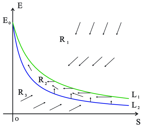
The first quadrant of the phase plane is divided into five regions as
where
| (24) | |||||
| (25) |
The whole process of the reaction can be drawn on the plane. Since decreases when increases, we can consider to be a function of .
| (26) |
The solutions with its initial condition on the curve will vertically enter the region . Then, the concentration of substrate decreases and that of enzyme increases. In fact, these solutions will stay in forever and finally approaches the singular point. For sufficiently large initial concentration of substrate, these solutions go almost horizontally in , but at last they will approach the singular point with a certain slope. Therefore, there is an inflection point on each of these solutions.
We have
| (27) |
Thus, the collection of inflection points satisfies , that is . As this system satisfies the existence and uniqueness condition of differential systems, any two different solutions will not intersect. Thus, the curve is just beneath the real process on the phase plane.
This is how we find the replacement .
5 Reasons for the replacement being much better
We will give reasons that (22) is a much better replacement of Michaelis-Menten curve in this section.
In [References], we have observed that there is a part of lying in the region which approximates the real process well. It is denoted as . In fact is the replacement of Michaelis-Menten curve. Next, we will show that is a better approximation of real reaction than which is the Michaelis-Menten curve (25). We only need to show that approximates real reaction better than does.
5.1 Comparison in the major process of a reaction
When the reaction begins, and would decrease until they pass through the curve . In this period of the reaction, neither Michaelis-Menten equation nor its replacement can approximate the solution well.
Here, the major process of a reaction means that and are in the region of excluding the end of the reaction. The following two subsections will show that gives a more approximation of the real reaction processes than (Michaelis-Menten curve) by numerical instances under different conditions.
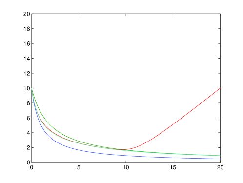
5.1.1 A case when QSSL condition violates
we choose , , , but . In this example the QSSL can not be used for is not sufficient large compared with . So may not be a good approximation of the solution. Before the reaction process approaches the region , both approximation of the solution are too bad. However, after the solution enters the region , gives a good approximation of the solution but doesn’t, c. f. Fig 2.
5.1.2 Cases when QSSL condition holds
We denote to be the solution with initial condition that , to be the explicit form of approximate solution and to be the explicit form of approximate solution . is greater than for all , which is proved in Appendix 6.1. is smaller than when , which is proved by Lemma 3 in [References]. Here, is the time the real process touches the curve . That is to say, after the reaction enters the region , the real process lies between these two approximations. We choose , , , and as the second example. In this example the QSSL can be used, so is a good approximation of the solution. During the reaction process, when or , the difference between and is less than the difference between and . That is to say is a better approximation of the solution after the initial transient period, i. e. less than 0.03.
We have also done another 250 numerical experiments. , and are chosen from , and , or . In each case, we divide into 7 equal pieces with 6 point, which we denote from small to large as . We calculate the distances of and and the distances of and . Table 1 shows the rate of these two numbers at the six points. These show that the curve approximate the solution better, and the smaller is the better does.
5.2 Comparison near the ends of the reactions
Our new equation , that is , approaches the end of reactions with a tangent line same to that of the reaction processes, while Michaelis-Menten curve does not. The following is the proof.
can be regarded as a graph of a function taking as independent variable and as dependent variable. The explicit form is given in Appendix 7.3. Rewrite as . Divide each side of the equation by and let . Then,
| (28) |
Solving it, we get
| (29) |
where the other root is dropped for the slope must be negative. This slope is just the slope of the solution entering the point . Thus, this part of give well approximation of even when is very small. So, we confirm this part of is a better approximation of a real reaction.
5.3 Comparison of the behaviors for large
In [References], we saw that almost coincide with when is sufficiently large. In fact, this can be proved. equals to . Let be the point on and on . Then, and . Thus, there must be one point between and such that . This proved that for each there is a point of curve lies in . In fact, there is only one. The proof is given in Appendix 7.3.
Moreover, we can prove that, as , . Since
it can be proved that
| (30) |
For
| (31) |
| (32) |
and
(30) can be written as
| (33) |
Letting on both side of (33),
for when .
Thus, there is a part of in region asymptotically approaching to when approaches .
implies . These together with (34) yields .
6 Application
The above section has shown that the curve approximates the trajectory of the reaction (1) better than the curve does. In this section, we will show that not only gives more information about the relationships among the three rate constants but also gives more accurate evaluations of these constants.
6.1 gives more information about the rate constants
For convenience, we repeat and here again as
Rearranging the items of the right side of yields that
By comparing equations and , we find that given some values of , we can calculate all the three values of , and up to a common multiplier by equation , but we only get two values of and up to a common multiplier by equation . In other words, only contains the information about the Michaelis constant as a whole, but contains the information of and , which also yield Michaelis constant by .
Moreover, by including an additional equation
| (35) |
This is just (6), from which can be measured, only provides the information about and , while provides that of all the three rate constants , and .
6.2 gives more accurate evaluations of the rate constant
As an example, we design a numerical experiment to show that compared with , not only gives more information about the relationships among the three rate constants but also gives more accurate evaluations of these constants. In the example, we set the rate constants as , and , and the initial concentrations of enzyme and substrate as and . Some points of are measured on the trajectory of the reaction, and then the results are calculated by and , respectively. All the results are listed in Table (2).
In table (2), we only list the concentrations of substrate, and do not list the corresponding concentrations of enzyme for brevity. means that the concentrations of substrate are measured from to with a step length . After measured these values of and their corresponding values of , can be calculated by and , respectively.
For different sets of points as chosen in table (2), is always closer to its exact value than . It is even the case, when there are only two points in the set, such as and .
Another phenomena observed from this table is that for both equations and , is more accurate when the data set is measured closer to the core region of the steady state of the reaction. Such a phenomena also gives another support that both and approximate the real reaction well at the quasi-steady state, moreover is better than .
If is measured by equation (6), then and are all known due to equation . In this example, we assume that , and hence, the estimated values of and are listed in the table, too.
Now, we have completely shown that compared with , not only gives more information about the relationships among the three rate constants but also gives more accurate evaluations of these constants. Thus, we claim that is a better replacement of Michaelis-Menten curve, and combined with (6) gives a better replacement of Michaelis-Menten equation.
7 Conclusion
In this article, we propose another curve that can replace the Michaelis-Menten curve and another equation that can replace the Michaelis-Menten equation. We used this new curve to estimate all the rate constants of the basic enzyme kinetics model. Results show that this replacement does very well. The Michaelis-Menten curve only gives information about . The Michaelis-Menten equation, which is derived by combining Michaelis-Menten curve and (6), only gives information about and . By contrasting to Michaelis-Menten curve, the replacement curve gives more information. And then, the replacement equation gives information about , and . Numerical experiments show that these replacements not only give more information about the relationships among the three rate constants but also give more accurate evaluations of these constants.
We did not give the mathematical meaning and reasoning that the replacement curve gives better approximate than Michaelis-Menten curve during the major process. Instead, we only give some numerical examples. We hope to do so in future work.
8 Appendix
8.1 in the initial transient period of a reaction
To obtain the Michaelis-Menten equation, (20) is assumed in former literatures. Here, we prove it under the conditions in QSSLs. That is to say if is much more larger than , is nearly equal to when . To be more precise and rigorous, we state it as a lemma below.
Lemma: Given and any small positive number , there is a proper positive number such that will be less than after a fast initial period less than , and keep this state until , if . Moreover, , for .
Proof: The first part of the theorem is just the QSSL2. According to Lemma 3 in [References], for . For equation (3),
| (36) |
Because of QSSL2, we could find and satisfies the following two statements, respectively. Given and any small positive number , there is a proper positive number such that will be less than after a fast initial period less than , and keep this state until , if . Given any small positive number , there is a proper positive number such that will be less than after a fast initial period less than and keep this state until , if . Choose such that and . Then, if , the first statement of the theorem is proved. Moreover, for (36)
| (37) |
when . This completes the proof.
Now
because , and can be arbitrarily small.
8.2 The convexity of
The solution do not have any inflection point at all, i. e. do not go across and lies above . Assume is a solution of system (10), and at time it intersects with at . Consider . Differentiate it with respect to , and note that , :
| (38) |
For simplicity, we write as , as , as , as and as . Simple calculation shows that
| (39) |
and
| (40) |
As ,
| (41) |
at point . By putting (39), (40) and (41) in (38),
| (42) |
For (LABEL:reginor2), . Therefore, if the solution of (10) has one point in the region satisfying , then for . We have proved that , where is on . Assume at time , reached the curve . Thus, . For continuity, there is a , such that for any , is in the region and . Then, for . Moreover, for , i. e. , can be verified by straight calculation. According to (27), is convex.
8.3 The explicit form
In this subsection, we talk about the explicit form of the curve . is a three degree equation of . Thus, for each , there are at most three real solutions of . We have proved that there is at least one solution of in the region for any . As in Section 3.2, we have proved that and . Note that,
| (43) |
for any . Thus, when is positively sufficiently large, . And when is negatively sufficiently large, . For the continuity of , there is at least one real solution greater than and there is at least one real solution less than . We have already found three solutions of when , so there are exact three solutions of when . The explicit form of all these three solutions, denoted by , and , can be given in mathematics.
The three solutions of the equation are
,
and
.
In this problem, , , and .
We have proved that all the three solutions are real, so we should decide which one represent the curve .
We choose , , , and . Then, , and . Therefore, is the right one in the region . Because , and are continuous functions of , , , and , and , and can not coincide for any , , , and , we can conclude that is the explicit form of , i. e. the replacement of the Michaelis-Menten equation.
Acknowledgments
This work is partially supported by a National Key Basic Research Project of China (2011CB302400), by National Natural Science Foundation of China (11301518) and by the National Center for Mathematics and Interdisciplinary Sciences, CAS.
References
-
[1]
Voet, D., J. G. Voet
and C. W. Pratt. Fundamentals of Biochemistry. John Wiley & Sons Inc, 1999.
-
[2]
Brown, A. J., 1902. Enzyme action. J. Chem. Soc. 81, 373–386.
-
[3]
Henri, V., 1902. Thorie gnrale de
quelques diastases. C. R. H. Acad. Sci. Paris 135, 916–919.
-
[4]
Schnell, S., Chappell,
M. J., Evans, N. D. and Roussel, M. R., 2006. The mechanism
distinguishability problem in biochemical kinetics: The
single-enzyme, single-substrate reaction as a case study. C. R.
Biologies 329, 51–61.
-
[5]
Briggs, G. E., J. B. S. Haldane, 1925.
A note on the kinetics of enzyme action. Biochem. J. 19, 338–339.
-
[6]
Fersht, A. R. Enzyme Structure and Mechanism. Freeman, 1985.
-
[7]
Schulz, A. R. Enzyme Kinetics: From Diastase to Multi-enzyme
Systems. Cambridge University Press, 1994.
-
[8]
Xie, X. S. and H. P. Lu, 1999. Single-molecule enzymology.
J. Biol. Chem. 274, 15967–15970.
-
[9]
Qian, H. and E. L. Elson, 2002. Single-molecule enzymology:
stochastic Michaelis-Menten kinetics. Biophys. Chem. 101–102: 565–576
-
[10]
Arnyi, P.;
J. Tth, 1977. A full stochastic description of the
Michaelis-Menten reaction for small systems. Acta Biochimica et
Biophysica Academiae Scientificarum Hungariae 12 (4), 375–388.
-
[11]
English, B. P., W. Min, A. M. van Oijen,
K. T. Lee, G. B. Luo, H. Y.Sun, B. J. Cherayil, S. C. Kou, and X. S.
Xie, 2006. Ever-fluctuating single enzyme molecules:
Michaelis-Menten equation revisited. Nat. Chem. Biol. 2, 87–94.
-
[12]
Lineweaver, H. and D. Burk, 1934.
The determination of enzyme dissociation constants. J. Am. Chem. Soc. 56, 658–666.
-
[13]
Dowd, J. E. and D. S. Riggs, 1965. A comparison of estimates of
Michaelis-Menten kinetic constants from various linear transformations. J. Biol. Chem 240, 863–869.
-
[14]
Chan, W. W.-C., 1995. Combination plots as graphical tools in the
study of enzyme inhibition. Biochem. J. 311 (Pt 3), 981–985.
-
[15]
Ritchie, R. J. and T. Prvan, 1996. A simulation study on designing
experiments to measure the of the Michaelis-Menten kinetics
curves. J. Theor. Biol. 178, 239–254.
-
[16]
Segel, I. H. Enzyme kinetics: Behavior and analysis of rapid
equilibrium and steady-state enzyme systems. Wiley, New York,
1975.
-
[17]
Dixon, M. and E. C. Webb. Enzymes. Academic Press, New York, 1979.
-
[18]
Schnell, S. and C. Mendoza, 1997. Closed form solution for
time-dependent enzyme kinetics. J. Theor. Biol. 187, 207–212.
-
[19]
Banghe Li, Yuefeng Shen and Bo Li, 2008. Quasi-Steady State Laws in Enzyme Kinetics.
J. Phys. Chem. A 112 (11), 2311–2321.
-
[20]
Segel, L. A. and M. Slemrod, 1989. The quasi-steady-state
assumption: a case study in perturbation. SIAM Rev. 31, 446–477.
-
[21]
Banghe Li, Bo Li and Yuefeng Shen. An improved method to measure all
rate constants in the simplest enzyme kinetics model (Accepted).
-
[22]
Banghe Li, Bo Li and Yuefeng Shen, 2009. A novel approach to measure
all rate constants in the simplest enzyme kinetics model.
J. Math. Chem. 46: 290-301.
-
[23]
Farkas, M. Dynamical models in biology. Academic Press, 2001.
-
[24]
Murray, J. D., Mathematical Biology. 3rd ed. in 2 volumes:
Mathematical Biology: I. An Introduction (551 pages), 2002;
Mathematical Biology: II. Spatial Models and Biomedical Applications
(811 pages), 2003.
-
[25]
Hirsch, M. W. and S. Smale. Differential equations, dynamical
systems, and linear algebra. Academic Press. Inc., New York, 1974.
-
[26]
Witold Hurewicz. Lectures on Ordinary Differential Equations. John Wiley and Sons, New York, 1958.
-
[27]
Schnell, S. and P. K. Maini, 2003. A century of enzyme kinetics:
Reliability of the and estimates. Comments on Theoretical Biology. 8, 169–187.
-
[28]
Segel, L. A., 1988. On the validity of the steady-state assumption
of enzyme kinetics. Bull. Math. Biol. 50, 579–593.
Figure 1: The - phase plane. Figure 2: gives a good approximation of the solution after the solution enters the region . Table 1: 250 numerical experiments. Table 2: Rate constants estimated by or . The first column indicates the measured concentrations of the substrate during the reaction process, and the corresponding concentrations of enzyme is determined by , so we do not show them explicitly. means that the concentrations are measured from to with step length . denotes the Michaelis constant estimated by , denotes the estimated by , and denote and estimated by , if is provided. Here, we assume that is exactly estimated by equation (35).
| 1 | 1 | 1 | 40 | 0.5 | 1360.849 | 978.494 | 659.542 | 404.013 | 211.969 | 83.724 |
|---|---|---|---|---|---|---|---|---|---|---|
| 1 | 1 | 3 | 40 | 0.5 | 1607.115 | 1190.643 | 837.895 | 549.093 | 324.898 | 168.645 |
| 1 | 1 | 5 | 40 | 0.5 | 1880.447 | 1430.567 | 1045.033 | 724.584 | 471.446 | 296.762 |
| 1 | 1 | 7 | 40 | 0.5 | 2182.374 | 1700.043 | 1283.124 | 933.340 | 655.858 | 476.536 |
| 1 | 1 | 9 | 40 | 0.5 | 2514.348 | 2000.800 | 1554.320 | 1178.212 | 882.388 | 716.419 |
| 1 | 3 | 1 | 40 | 0.5 | 532.045 | 393.568 | 276.394 | 180.568 | 106.235 | 54.160 |
| 1 | 3 | 3 | 40 | 0.5 | 623.350 | 473.711 | 345.536 | 239.036 | 154.855 | 96.309 |
| 1 | 3 | 5 | 40 | 0.5 | 724.132 | 563.671 | 424.992 | 308.626 | 216.180 | 155.887 |
| 1 | 3 | 7 | 40 | 0.5 | 834.896 | 664.039 | 515.482 | 390.276 | 291.599 | 235.622 |
| 1 | 3 | 9 | 40 | 0.5 | 956.131 | 775.389 | 617.712 | 484.918 | 382.495 | 338.216 |
| 1 | 5 | 1 | 40 | 0.5 | 372.294 | 282.761 | 206.082 | 142.360 | 91.916 | 56.441 |
| 1 | 5 | 3 | 40 | 0.5 | 432.776 | 336.705 | 253.673 | 183.969 | 128.482 | 91.841 |
| 1 | 5 | 5 | 40 | 0.5 | 499.232 | 396.886 | 307.883 | 232.825 | 173.536 | 139.448 |
| 1 | 5 | 7 | 40 | 0.5 | 571.961 | 463.651 | 369.141 | 289.489 | 227.906 | 200.886 |
| 1 | 5 | 9 | 40 | 0.5 | 651.252 | 537.344 | 437.867 | 354.516 | 292.417 | 277.761 |
| 1 | 7 | 1 | 40 | 0.5 | 308.005 | 239.517 | 180.320 | 130.602 | 90.937 | 64.393 |
| 1 | 7 | 3 | 40 | 0.5 | 355.468 | 282.472 | 218.981 | 165.402 | 122.974 | 98.218 |
| 1 | 7 | 5 | 40 | 0.5 | 407.406 | 330.128 | 262.678 | 205.787 | 161.686 | 142.000 |
| 1 | 7 | 7 | 40 | 0.5 | 464.028 | 382.732 | 311.712 | 252.155 | 207.663 | 196.886 |
| 7 | 5 | 9 | 40 | 0.5 | 1905.853 | 1368.871 | 921.202 | 562.884 | 294.032 | 115.236 |
| 7 | 7 | 1 | 40 | 0.5 | 1261.696 | 893.181 | 588.432 | 347.446 | 170.216 | 56.703 |
| 7 | 7 | 3 | 40 | 0.5 | 1293.832 | 920.402 | 610.742 | 364.855 | 182.747 | 64.456 |
| 7 | 7 | 5 | 40 | 0.5 | 1326.463 | 948.129 | 633.572 | 382.803 | 195.852 | 72.877 |
| 7 | 7 | 7 | 40 | 0.5 | 1359.591 | 976.365 | 656.927 | 401.299 | 209.543 | 81.987 |
| 7 | 7 | 9 | 40 | 0.5 | 1393.227 | 1005.120 | 680.817 | 420.352 | 223.832 | 91.812 |
| 7 | 9 | 1 | 40 | 0.5 | 1004.972 | 714.795 | 474.213 | 283.225 | 141.824 | 49.985 |
| 7 | 9 | 3 | 40 | 0.5 | 1030.374 | 736.374 | 491.974 | 297.178 | 151.996 | 56.486 |
| 7 | 9 | 5 | 40 | 0.5 | 1056.165 | 758.350 | 510.144 | 311.557 | 162.624 | 63.526 |
| 7 | 9 | 7 | 40 | 0.5 | 1082.346 | 780.727 | 528.727 | 326.368 | 173.717 | 71.122 |
| 9 | 5 | 7 | 20 | 0.5 | 632.410 | 458.999 | 313.794 | 196.824 | 108.175 | 48.333 |
| 9 | 5 | 9 | 20 | 0.5 | 657.240 | 480.424 | 331.837 | 211.529 | 119.657 | 57.071 |
| 9 | 7 | 1 | 20 | 0.5 | 416.007 | 297.340 | 198.796 | 120.367 | 62.035 | 23.724 |
| 9 | 7 | 3 | 20 | 0.5 | 432.973 | 311.831 | 210.819 | 129.935 | 69.181 | 28.595 |
| 9 | 7 | 5 | 20 | 0.5 | 450.325 | 326.725 | 223.264 | 139.952 | 76.824 | 34.092 |
| 9 | 7 | 7 | 20 | 0.5 | 468.080 | 342.036 | 236.146 | 150.433 | 84.981 | 40.245 |
| 9 | 7 | 9 | 20 | 0.5 | 486.247 | 357.774 | 249.473 | 161.389 | 93.667 | 47.083 |
| 9 | 9 | 1 | 20 | 0.5 | 335.698 | 241.688 | 163.326 | 100.608 | 53.515 | 21.984 |
| 9 | 9 | 3 | 20 | 0.5 | 349.216 | 253.282 | 173.005 | 108.384 | 59.425 | 26.189 |
| 9 | 9 | 5 | 20 | 0.5 | 363.046 | 265.201 | 183.022 | 116.521 | 65.737 | 30.907 |
| 9 | 9 | 7 | 20 | 0.5 | 377.191 | 277.447 | 193.383 | 125.026 | 72.459 | 36.160 |
| 9 | 9 | 9 | 20 | 0.5 | 391.664 | 290.032 | 204.100 | 133.911 | 79.607 | 41.973 |
| S | |||||
|---|---|---|---|---|---|
| 3:0.1:19 | 0.996345 | 0.999979 | 0.3052 | 0.1052 | 0.2000 |
| 3:0.5:19 | 0.996243 | 0.999978 | 0.3055 | 0.1055 | 0.2000 |
| 3:1.0:19 | 0.996112 | 0.999977 | 0.3057 | 0.1057 | 0.2000 |
| 3:2.0:19 | 0.995837 | 0.999975 | 0.3063 | 0.1063 | 0.2000 |
| 3:4.0:19 | 0.995253 | 0.999972 | 0.3073 | 0.1072 | 0.2000 |
| 3:8.0:19 | 0.994059 | 0.999972 | 0.3083 | 0.1083 | 0.2000 |
| 3:16 :19 | 0.991973 | 0.999978 | 0.3088 | 0.1088 | 0.2000 |
| 10:0.1:19 | 0.998506 | 0.999996 | 0.3017 | 0.1017 | 0.2000 |
| 10:0.5:19 | 0.998495 | 0.999996 | 0.3017 | 0.1017 | 0.2000 |
| 10:1.0:19 | 0.998481 | 0.999996 | 0.3018 | 0.1018 | 0.2000 |
| 10:2.0:19 | 0.998374 | 0.999995 | 0.3019 | 0.1019 | 0.2000 |
| 10:4.0:19 | 0.998320 | 0.999995 | 0.3019 | 0.1019 | 0.2000 |
| 10:8.0:19 | 0.998215 | 0.999996 | 0.3020 | 0.1020 | 0.2000 |
| 16:0.1:19 | 0.999024 | 0.999998 | 0.3011 | 0.1011 | 0.2000 |
| 16:0.5:19 | 0.999022 | 0.999998 | 0.3011 | 0.1011 | 0.2000 |
| 16:1.0:19 | 0.999020 | 0.999998 | 0.3011 | 0.1011 | 0.2000 |
| 16:2.0:19 | 0.998967 | 0.999998 | 0.3011 | 0.1011 | 0.2000 |