Thermodynamics of an exactly solvable confining quark model

Abstract

The grand partition function of a model of confined quarks is exactly calculated at arbitrary temperatures and quark chemical potentials. The model is inspired by a softly BRST-broken version of QCD and possesses a quark mass function compatible with nonperturbative analyses of lattice simulations and Dyson-Schwinger equations. Even though the model is defined at tree level, we show that it produces a nontrivial and stable thermodynamic behaviour at any temperature or chemical potential. Results for the pressure, the entropy and the trace anomaly as a function of the temperature are qualitatively compatible with the effect of nonperturbative interactions as observed in lattice simulations. The finite density thermodynamics is also shown to contain nontrivial features, being far away from an ideal gas picture.

I Introduction

The study of the infrared behavior of non-Abelian gauge theories, like Quantum Chromodynamics, presents a remarkable task for theoretical physics. The strongly-coupled nonperturbative nature of infrared phenomena greatly undermines our ability to access the physical properties of the theory in an analytical way. One general question raised in this context concerns the description of the degrees of freedom in a confining theory. Confinement of the perturbative excitations associated with the fundamental fields means, among other features, that these degrees of freedom do not appear in the physical spectrum of the theory as asymptotic states. The physical spectrum in this case is given by bound states associated with composite fields of the theory. The fundamental problem is thus to understand how the perturbative degrees of freedom disappear from the spectrum and how this is reflected in an action formulation written in terms of them.

A very important tool in identifying the physical space of states in a gauge theory is the BRST symmetry Becchi:1975nq ; Tyutin:1975qk . In a BRST invariant theory, the physical states are defined by the cohomology of the nilpotent BRST operator that acts on the fundamental fields. However, this is strictly valid only at the perturbative level. In fact, the whole construction of the BRST formalism in a gauge theory can be traced back to the Faddeev-Popov procedure of gauge fixing. Since it has long been known that this procedure ceases to be valid at the nonperturbative level Gribov:1977wm , there is no strict necessity to expect that the BRST symmetry survives in the infrared regime. Indeed, there is strong evidence coming from lattice studies that the BRST symmetry is broken at low energies Cucchieri:2014via . This is in tune with the expectations for a confining theory: the survival of the original BRST symmetry would allow for a definition of the physical spectrum, by its cohomology, in terms of the fundamental fields, thus contradicting confinement.

It is therefore expected that the description of the original perturbative degrees of freedom is modified in the infrared. This seems to be exactly what happens in pure gauge theories according to lattice results concerning the Yang-Mills gauge field and ghost propagators in the Landau gauge Cucchieri:2007rg ; Cucchieri:2008fc ; Cucchieri:2011ig : positivity violation is observed for the gluon two-point function. It is well-known Peskin:1995ev ; Weinberg:1995mt that the two-point function of a physical field is directly related to the probability of propagation of the associated asymptotic state. Therefore, positivity violation, as observed for lattice gluons, hinders the probabilistic interpretation of the two-point function in terms of propagating particles, being consistent with confinement in the sense of absence of colored states from the spectrum. This is the confinement criterion we adopt (more discussion can be found in e.g. the reviews Alkofer:2000wg ; Brambilla:2014jmp ).

The numerical data also point to gluon propagator that tends to a constant value in the infrared, while the ghost propagator has the behavior of a free particle. In the context of the Schwinger-Dyson equations, this is called the decoupling solution Aguilar:2008xm . The theoretical description of these results in the continuum has been proposed to be provided by an effective action in the so-called refined Gribov-Zwanziger (RGZ) formalism Dudal:2007cw ; Dudal:2008sp ; Dudal:2011gd . The RGZ action is renormalizable and displays a softly broken BRST symmetry. One very important feature of this formalism is the guarantee that the quantum ultraviolet behavior of the theory is under control and the – very successful – original perturbative Yang-Mills framework is recovered at high energies.

The RGZ action describes a pure gluonic theory and its construction has the geometrical guidance of the original Gribov observations about the configuration space of the gauge fields. Its action effectively describes the restriction of the path integral measure to a region without the infinitesimal Gribov gauge copies, while also taking into account the formation of condensates. The resulting action has tree-level propagators that describe very well the lattice data at zero and finite temperature Cucchieri:2010xr ; Bornyakov:2011fn and can be used to obtain consistent estimates of the masses of glueball states with different quantum numbers Dudal:2010cd ; Dudal:2013wja .

An interesting development is that lattice data on propagators suggest a similar behavior for the gauge-interacting matter fields, displaying positivity violation Parappilly:2005ei , as observed for the gluon fields. Furthermore, the theoretical description of these degrees of freedom in the infrared has been conjectured to have the same structure as for the gluon, with an action whose tree-level propagators reproduce very well the lattice data, also displaying softly broken BRST symmetry Capri:2014bsa . It should be noticed, however, that in the case of matter fields a geometrical interpretation of the modified action as a restriction in the configuration space of the fields is lacking.

This set of affairs led us to expect that a possible signature of confinement would be the soft breaking of the BRST symmetry. In fact this relation has been explored in many works Baulieu:2008fy ; Dudal:2009xh ; Sorella:2009vt ; Sorella:2010it ; Capri:2010hb ; Dudal:2012sb ; Reshetnyak:2013bga . The idea is that confined degrees of freedom are described by an effective action with a BRST-breaking soft term. Interestingly, the breaking of the BRST invariance may have a connection with chiral symmetry breaking, since the currently known formulations of soft BRST breaking in the quark sector always imply chiral symmetry breaking Baulieu:2009xr ; Dudal:2013vha and thus dynamical mass generation in the deep infrared seems to be intimately related to BRST breaking Capri:2014bsa . In this sense, one may hope that the investigation of the nonperturbative breaking of the BRST symmetry may shed some light on a long-standing puzzle in the QCD phase structure: the apparent and unexplained link between confinement and chiral symmetry breaking.

Several effective models of QCD present in the literature address the relation between chiral symmetry breaking and confinement. Two important prototype models extensively explored to address the question of chiral symmetry breaking in the strong interactions are the Nambu-Jona-Lasinio (NJL) and the Quark Meson (QM) models Nambu:1961tp ; GellMann:1960np , generically called chiral models. On one hand, chiral symmetry breaking and restoration is, in chiral models, a result of the interaction of the quark sector either to itself (in a four-fermion vertex, as in the NJL model) or to meson fields (as in the QM model). On the other hand, as an attempt to take into account the physics of confinement, one can introduce a Polyakov loop field coupled to quarks Meisinger:1995ih ; Fukushima:2003fw ; Megias:2004hj ; Ratti:2005jh ; Schaefer:2007pw ; Schaefer:2009ui . Within the Polyakov loop extended NJL (PNJL) and QM (PQM) models, the Polyakov loop field effectively encodes the gauge field as an external background that interacts with the quark degrees of freedom, so that the deconfinement transition may be studied in this context as a (static) Landau-Ginzburg system coupled to the chiral model. In spite of their interaction with the Polyakov loop, the quark degrees of freedom in both the PNJL and PQM models physically correspond to asymptotic states, not to confined ones. This is so because their two-point functions only have poles on the real axis and thus respect the Osterwalder-Schrader’s axiom of reflection positivity Osterwalder:1973dx , guaranteeing the establishment of a standard probabilistic description of propagation of asymptotic quarks, in contradiction with real-world QCD.

A possible way to extend the NJL model is to include a nonlocal current-current interaction kernel General:2000zx ; Contrera:2010kz ; Benic:2012ec ; Benic:2013eqa . As a result, complex quark masses may appear, indicating confinement in the sense we discussed before. However, due to its four-fermion interaction, the nonlocal NJL model is not renormalizable, similarly to its local version. Besides, it also leads to unstable thermodynamic behavior Benic:2012ec ; Benic:2013eqa ; Loewe:2014vna .

In the last years, some works have explored the thermodynamic properties of softly BRST broken pure gauge systems (see, for example, Zwanziger:2004np ; Zwanziger:2006sc ; Lichtenegger:2008mh ; Fukushima:2013xsa ; Reinhardt:2012qe ; Reinhardt:2013iia ). In this paper, we explore thermodynamic properties of a model of quarks with soft BRST breaking. As discussed above, this model is expected to describe the infrared properties of confined (positivity-violating) quarks, while keeping compatibility with ultraviolet QCD properties. Indeed, the analytical propagator of the model fits well the available lattice data Dudal:2013vha and the model has been proven to be renormalizable Baulieu:2009xr , reducing to perturbative quarks in the ultraviolet regime. Our goal here is to show not only that soft BRST breaking in the quark sector implies a well-defined macroscopic behaviour, but also that the tree level model is capable of predicting nontrivial features, being in general qualitatively compatible with the effect of nonperturbative interactions as observed in lattice data. Furthermore, the instabilities present in the nonlocal NJL model are absent from our setup.

This work is organized as follows. Section II presents the action defining the model. In Section III the exact partition function is computed within the imaginary-time formalism. In section IV we obtain the thermodynamic quantities and present our results for the distribution function, the pressure, the entropy, and the trace anomaly. Our conclusions are discussed in Section V.

II The action of the quark model with soft BRST breaking

Following the discussion of Baulieu:2009xr , let us briefly review how a model with soft breaking of the BRST symmetry can be obtained from an extension of the QCD lagrangian. We start from the gauge-fixed lagrangian density in an euclidean space of dimension 4,

$${\cal L}_{QCD}=\frac{1}{4}F_{\mu\nu}^{a}F_{\mu\nu}^{a}+\bar{\psi}_{\alpha}^{i}[i(\gamma_{\mu})_{\alpha\beta}D_{\mu}^{ij}-m_{0}\delta_{\alpha\beta}\delta^{ij}]\psi_{\beta}^{j}+ib^{a}\partial_{\mu}A_{\mu}^{a}+\bar{c}^{a}\partial_{\mu}D_{\mu}^{ab}c^{b},$$ (1)

where $F_{\mu\nu}^{a}=\partial_{\mu}A_{\nu}^{a}-\partial_{\nu}A_{\mu}^{a}+gf^{abc}A_{\mu}^{b}A_{\nu}^{c}$ is the field strength and $D^{ij}_{\mu}=\delta^{ij}\partial_{\mu}-ig(T^{a})^{ij}A_{\mu}^{a}$ is the covariant derivative. The indices $(a,b,\dots,h)=1,\dots,N_{c}^{2}-1$ correspond to adjoint representation and $(i,j,\dots)=1,\dots,N_{c}$ correspond to fields in the fundamental representation of $SU(N_{c})$. The greek indices $(\alpha,\beta,\dots)=1,2,3,4$ denote spinor indices while $(\mu,\nu,\dots)=1,2,3,4$ regard euclidean space indices. For more details on notational conventions, the reader is referred to Ref. LeBellac:book .

One very important feature of (1) is its invariance under BRST transformations Becchi:1975nq ; Tyutin:1975qk ,

$$sA_{\mu}^{a}=-D_{\mu}^{ab}c^{b}$$

$$s\psi_{\alpha}^{i}=-igc^{a}(T^{a})^{ij}\psi^{j}_{\alpha}$$

$$s\bar{\psi}_{\alpha}^{i}=-ig\bar{\psi}_{\alpha}^{j}c^{a}(T^{a})^{ji}$$

$$sc^{a}=\frac{1}{2}gf^{abc}c^{b}c^{c}$$

$$s\bar{c}^{a}=ib^{a}$$

$$sb^{a}=0$$ (2)

which is crucial for its multiplicative renormalizability. As an intermediate step in the definition of the model, let us introduce two BRST doublets $(\xi^{i},\theta^{i})$ and $(\eta^{i},\lambda^{i})$ of auxiliary fields (and their hermitian conjugate fields) that transform as

$$s\xi_{\alpha}^{i}=\theta_{\alpha}^{i},\;\;\;\;s\theta_{\alpha}^{i}=0$$

$$s\eta_{\alpha}^{i}=\lambda_{\alpha}^{i},\;\;\;s\lambda_{\alpha}^{i}=0.$$ (3)

The addition of the BRST invariant action

$$S_{\xi\lambda} = s\int d^{4}x\left[-\bar{\eta}^{i}_{\alpha}\partial^{2}\xi_{\alpha}^{i}+\bar{\xi}^{i}_{\alpha}\partial^{2}\eta_{\alpha}^{i}+m^{2}(\bar{\eta}^{i}_{\alpha}\xi_{\alpha}^{i}-\bar{\xi}_{\alpha}^{i}\eta_{\alpha}^{i})\right]$$ (4)

$$= \int d^{4}x\left[-\bar{\lambda}_{\alpha}^{i}\partial^{2}\xi_{\alpha}^{i}-\bar{\xi}^{i}_{\alpha}\partial^{2}\lambda_{\alpha}^{i}-\bar{\eta}_{\alpha}^{i}\partial^{2}\theta_{\alpha}^{i}+\bar{\theta}_{\alpha}^{i}\partial^{2}\eta_{\alpha}^{i}+m^{2}\left(\bar{\lambda}^{i}_{\alpha}\xi_{\alpha}^{i}+\bar{\xi}_{\alpha}^{i}\lambda_{\alpha}^{i}+\bar{\eta}_{\alpha}^{i}\theta_{\alpha}^{i}-\bar{\theta}_{\alpha}^{i}\eta_{\alpha}^{i}\right)\right]$$

does not change the physical content of the theory. This can be easily checked by integrating the auxiliary fields, which trivially gives $1$. However, if one also adds to the action the coupling

$$S_{M}=\int d^{4}x\left[M_{1}^{2}(\bar{\xi}^{i}_{\alpha}\psi_{\alpha}^{i}+\bar{\psi}_{\alpha}^{i}\xi_{\alpha}^{i})-M_{2}(\bar{\lambda}_{\alpha}^{i}\psi_{\alpha}^{i}+\bar{\psi}_{\alpha}^{i}\lambda^{i}_{\alpha})\right]$$ (5)

between the auxiliary fields and the matter fields, the resulting action $S_{tot}=S_{QCD}+S_{\xi\lambda}+S_{M}$ is no longer BRST invariant. However, as shown in Baulieu:2009xr , this does not destroy the renormalizability of the theory once it corresponds to a soft breaking of the BRST symmetry. In other words, the theory modified by $S_{M}$ is equivalent to actual QCD in the ultraviolet.

Of course, the addition of (5) leads to changes of the theory in the infrared with respect to actual QCD and one might ask to what extent such a theory can correctly describe the infrared physics of QCD. Interestingly enough, BRST soft breaking terms can be dynamically generated. For example, gluon condensation may be incorporated in the action and serve as a starting point for an effective theory containing nonperturbative physics Baulieu:2008fy . Indeed, the presence of such condensates leads to a nontrivial infrared behavior of gluon and ghost propagators, which can be also observed in lattice simulations Cucchieri:2007rg ; Cucchieri:2008fc ; Cucchieri:2011ig . In the quark sector of the theory, the BRST breaking term (5) is conjectured to be a consequence of the condensation of the $\bar{q}q$ operator.

The physical meaning of the action $S_{tot}$ becomes clearer after integration in the auxiliary fields $(\xi,\bar{\xi})$, $(\eta,\bar{\eta})$, $(\theta,\bar{\theta})$, and $(\lambda,\bar{\lambda})$. As a result, due to the BRST breaking term $S_{M}$, one finds a nonlocal action

$$S_{nl}=\int d^{4}x\,\bar{\psi}_{\alpha}^{i}\left[i(\gamma_{\mu})_{\alpha\beta}\delta^{ij}\partial_{\mu}-\delta^{ij}\delta_{\alpha\beta}\left(\frac{2M_{1}^{2}M_{2}}{-\partial^{2}+m^{2}}+m_{0}\right)\right]\psi^{j}_{\beta}$$ (6)

for the quark sector, plus the minimal coupling to the gauge sector. As a first approximation in our model, we neglect the interaction between the gauge and the matter sectors, except through the nonperturbative term $S_{M}$. Notice that the usual local free fermion case can be recovered for $2M_{1}^{2}M_{2}\equiv M_{3}\rightarrow 0$.

In the vacuum, the tree level fermion propagator reads (with omission of color and Dirac indices)

$$S(p)=-\frac{\gamma_{\mu}p_{\mu}+M_{0}(p)}{p^{2}+M_{0}^{2}(p)},$$ (7)

where we defined the vacuum mass function

$$M_{0}(p)=\frac{2M_{1}^{2}M_{2}}{p^{2}+m^{2}}+m_{0}.$$ (8)

Such a quark mass function is compatible with lattice QCD calculations at zero temperature Parappilly:2005ei as well as with an analysis of the Dyson-Schwinger equations of the quark propagator Bhagwat:2003vw . The parameters $M_{3}\equiv 2M_{1}^{2}M_{2}$, $m^{2}$ and $m_{0}$ of the mass function (8) can be well fitted to the lattice results of Parappilly:2005ei , giving $M_{3}=0.196$GeV³, $m^{2}=0.639$GeV², and $m_{0}=0.014$GeV with $\chi^{2}/dof=1.18$ Dudal:2013vha . Notice also that the propagator (7) has two complex conjugate poles and a real pole. This can be interpreted as a sign of confinement, a property expected from strongly interacting particles at zero temperature.

Once the action of the quark sector

$$S_{q}=\int d^{4}x\,\bar{\psi}_{\alpha}^{i}[i(\gamma_{\mu})_{\alpha\beta}\partial_{\mu}-\delta_{\alpha\beta}m_{0}]\psi_{\beta}^{i}+S_{\xi\lambda}+S_{M}.$$ (9)

is quadratic in the fermion fields, it is possible to calculate the partition function exactly for arbitrary temperatures and chemical potentials. In the next section, we will calculate the grand canonical partition function of the theory defined by (9).

III The partition function : an exact computation

In order to calculate the partition function of the theory (9), we shall use standard techniques of finite temperature field theory in the Matsubara imaginary time formalism LeBellac:book ; KapustaGale . At finite temperature, the 0-direction is compactified ($\mathbb{R}\rightarrow\mathbb{S}^{1}\equiv[0,\beta)$), with $\beta\equiv 1/T$ and the fermion fields obey anti-periodic boundary conditions in imaginary time. As a consequence, the fermion fields can be written in terms of their Fourier transforms as

$$\psi(x_{4},{\bf x})=\sum_{n}\int\,\frac{d^{3}p}{(2\pi)^{3}}e^{-i{\bf p}\cdot{\bf x}}e^{-i\omega_{n}x_{4}}\tilde{\psi}(\omega_{n},{\bf p}),$$ (10)

and

$$\bar{\psi}(x_{4},{\bf x})=\sum_{m}\int\,\frac{d^{3}q}{(2\pi)^{3}}e^{-i{\bf q}\cdot{\bf x}}e^{-i\omega_{m}x_{4}}\tilde{\bar{\psi}}(\omega_{m},{\bf q}),$$ (11)

where $\omega_{n}=(2n+1)\pi T$ are Matsubara frequencies ($n\in\mathbb{Z}$).

The presence of a net quark charge requires a nonzero quark chemical potential $\mu$. Indeed, a Noether charge can be associated with a global $U(1)$ transformation of the type

$$\psi\rightarrow e^{-i\alpha}\psi,$$ (12)

with $\alpha\in\mathbb{R}$. It is crucial to notice that the action (9) is invariant under this transformation only if all the auxiliary fields also carry this same charge. The corresponding Noether current is then used to impose the grand canonical constraint on the hamiltonian of the theory. The calculation is straightforward but it must be carefully performed. The details of the derivation of the in-medium effective action for the quark fields are given in the Appendix (A).

After imposing the grand canonical constraint and integrating out the auxiliary fields and their respective momenta, the grand canonical partition function can then be written in the nonlocal form

$$Z(T,\mu) = {\rm Tr\,}\exp\left[-\beta\left(\hat{H}-\mu\hat{N}\right)\right]$$

$$= \int[D\bar{\psi}][D\psi]\exp\left[-\int_{0}^{\beta}d^{4}x\,{\cal L}_{nl}[\bar{\psi},\psi]\right]$$

where, omitting color and spinor indices,

$${\cal L}_{nl}=\bar{\psi}\left[\gamma_{4}\left(\partial_{4}-\mu\right)-i{\bf\gamma}\cdot\nabla+\frac{M_{3}}{-(\partial_{4}-\mu)^{2}-\nabla^{2}+m^{2}}+m_{0}\right]\psi.$$ (14)

That is, our calculation explicitly showed that the inclusion of the chemical potential simply amounts to the shift $\partial_{4}\rightarrow\partial_{4}-\mu$. It follows from (10) and (11) that

$$\int_{X}{\cal L}_{nl}=\sum_{n}\int\,\frac{d^{3}p}{(2\pi)^{3}}{\tilde{\bar{\psi}}}(-\omega_{n},-{\bf p})\left[\beta\left(-\gamma_{4}(i\omega_{n}+\mu)-{\bf\gamma}\cdot{\bf p}+M_{n,{\bf p}}(\mu)\right)\right]\tilde{\psi}(\omega_{n},{\bf p})$$ (15)

where

$$M_{n,{\bf p}}(\mu):=\frac{M_{3}}{-(i\omega_{n}+\mu)^{2}+{\bf p}^{2}+m^{2}}+m_{0}.$$ (16)

corresponds to the mass function (8) at finite temperature and chemical potential.

Being quadratic in the fermionic operators, the partition function can be formally integrated immediately, giving

$$Z(T,\mu)=\det_{p,D,f,c}\left[-\beta\gamma_{4}(i\omega_{n}+\mu)-\beta{\bf\gamma}\cdot{\bf p}+\beta M_{n,{\bf p}}(\mu)\right],$$ (17)

where the (full) determinant has to be taken with respect to the momentum (p), Dirac (D), flavor (f), and color (c) subspaces.

Let us follow the same steps as in, e.g., KapustaGale , in order to calculate the grand partition function (17). The determinant in flavor and color spaces are very simple, once all $N_{f}$ flavors and $N_{c}$ quark colors are on equal footing. This corresponds to taking the determinant in Dirac and momentum subspaces to the power $N_{c}N_{f}$. Furthermore, the Dirac determinant can be straightforwardly computed to be

$$\det_{D}\left[-\beta\gamma_{4}(i\omega_{n}+\mu)-\beta{\bf\gamma}\cdot{\bf p}+\beta M_{n,{\bf p}}(\mu)\right]=\beta^{4}\left[{\bf p}^{2}+M_{n,{\bf p}}^{2}(\mu)-(i\omega_{n}+\mu)^{2}\right]^{2}.$$ (18)

Before proceeding to the calculation of the determinant in momentum space, it is convenient to consider the logarithm of the partition function and use the operator identity $\log\det\hat{A}={\rm Tr\,}\log\hat{A}$ where, in momentum space, $\hat{A}\equiv\beta^{4}\left[{\bf p}^{2}+M_{n,{\bf p}}^{2}(\mu)+(\omega_{n}-i\mu)^{2}\right]^{2}$. The trace in momentum space correponds to summing over all Matsubara frequencies and all momenta. In the thermodynamic limit ($V\rightarrow\infty$),

$$\sum_{\bf p}(\cdots)\longrightarrow V\int\frac{d^{3}p}{(2\pi)^{3}}(\cdots)$$ (19)

As a result, we find

$$\log Z(T,\mu)=2VN_{c}N_{f}\sum_{n}\int\frac{d^{3}p}{(2\pi)^{3}}\log\beta^{2}\left[{\bf p}^{2}+M_{n,{\bf p}}^{2}(\mu)-(i\omega_{n}+\mu)^{2}\right].$$ (20)

Notice that the sum (20) is real although its integrand is not. Using that $\omega_{0}=-\omega_{-1}$, $\omega_{1}=-\omega_{-2}$ etc., it is not difficult to write (20) explicitly as a sum of real numbers by splitting the sum of Matsubara frequencies for $n\geq 0$ and $n\leq-1$. In order to continue the calculation, it is best to split Eq. (20) in two factors, adding and subtracting the $\mu=0$ contribution, so that

$$\frac{\log Z(T,\mu)}{2\beta VN_{c}N_{f}} = \sum\!\!\!\!\!\!\!\int\,\log\left\{\beta^{2}\left[{\bf p}^{2}+M_{n,{\bf p}}^{2}(0)+\omega_{n}^{2}\right]\right\}+\sum\!\!\!\!\!\!\!\int\,\log\left\{\frac{{\bf p}^{2}+M_{n,{\bf p}}^{2}(\mu)-(i\omega_{n}+\mu)^{2}}{{\bf p}^{2}+M_{n,{\bf p}}^{2}(0)+\omega_{n}^{2}}\right\}$$ (21)

$$\equiv \frac{\log Z(T,0)}{2\beta VN_{c}N_{f}}+\frac{\log Z^{(\mu)}(T,\mu)}{2\beta VN_{c}N_{f}},$$ (22)

where we used the standard sum-integral notation,

$$\sum\!\!\!\!\!\!\!\int\,(\cdots)\equiv T\sum_{n=-\infty}^{\infty}\int\frac{d^{3}p}{(2\pi)^{3}}(\cdots).$$ (23)

One interesting feature of the decomposition (21) is that only the term $\log Z(T,0)$ contains any divergencies. They are the same as those of the local theory at $T=0$ and therefore can be straightforwardly subtracted. The $\mu\not=0$ contribution is finite, as expected from the argument that the introduction of a chemical potential should not bring any new divergencies to the theory. For this reason, it can be calculated numerically and also has a closed expression in terms of elementary integrals in the limit of zero temperature.

For clarity, let us now separately discuss the calculations of the $\mu=0$ and $\mu\not=0$ contributions.

III.1 The $\mu=0$ contribution

In the standard calculation of the partition function of local free quarks of mass $m_{0}$ at $\mu=0$ (see, e.g., LeBellac:book ; KapustaGale ), one is lead to the calculation of the sum-integral

$$\log Z_{loc}(T,0)=2N_{c}N_{f}\beta V\sum\!\!\!\!\!\!\!\int\,\log\left\{\beta^{2}\left[\omega_{n}^{2}+\omega^{2}\right]\right\},$$ (24)

where $\omega=\sqrt{{\bf p}^{2}+m_{0}^{2}}$. After subtractions of $T$- and $\mu$-independent (infinite) constants, one arrives at the final expression

$$\log Z_{loc}(T,0)=2N_{c}N_{f}\beta V\int\frac{d^{3}p}{(2\pi)^{3}}\left[\omega+2T\log\left(1+e^{-\beta\omega}\right)\right].$$ (25)

It is quite straightforward to show that the calculation of

$$\log Z(T,0)=2\beta VN_{c}N_{f}\sum\!\!\!\!\!\!\!\int\,\log\left\{\beta^{2}\left[{\bf p}^{2}+M_{n,{\bf p}}^{2}(0)+\omega_{n}^{2}\right]\right\}$$ (26)

can be reduced to the sum of four terms which are each formally identical to (24). Indeed, using Eq. (16), it is possible to write the argument of the logarithm in (26), $Arg$, as a ratio of two polynomials,

$$Arg:=\frac{\beta^{2}\left[({\bf p}^{2}+m_{0}^{2}+\omega_{n}^{2})({\bf p}^{2}+m^{2}+\omega_{n}^{2})^{2}+2M_{3}m_{0}({\bf p}^{2}+m^{2}+\omega_{n}^{2})+M_{3}^{2}\right]}{({\bf p}^{2}+m^{2}+\omega_{n}^{2})^{2}}\equiv\beta^{2}\frac{P_{3}(\omega_{n}^{2})}{({\bf p}^{2}+m^{2}+\omega_{n}^{2})^{2}}$$ (27)

where the third degree polynomial $P_{3}(\omega_{n}^{2})$ can be factored out as

$$P_{3}(\omega_{n}^{2})=(\omega_{n}^{2}+\varphi_{1}^{2})(\omega_{n}^{2}+\varphi_{2}^{2})(\omega_{n}^{2}+\varphi_{3}^{2}),$$ (28)

with $-\varphi_{i}^{2}$ $(i=1,2,3)$ the three roots of $P_{3}$. In general, the roots of a third degree polynomial of real coefficients are one real number and a couple of complex conjugate numbers. This is indeed the case for our parameter set, as should be evident from the presence of complex poles in the propagator, i.e., complex masses. The three roots can be explicitly calculated as functions of ${\bf p}^{2}$ and the parameters $M_{3}$, $m^{2}$, and $m_{0}$. Substituting back in (26), we have

$$\log Z(T,0)=2N_{c}N_{f}\beta V\sum\!\!\!\!\!\!\!\int\,\left\{\sum_{i=1}^{3}\log\left[\beta^{2}\left(\omega_{n}^{2}+\varphi_{i}^{2}\right)\right]-2\log\left[\beta^{2}\left(\omega_{n}^{2}+{\bf p}^{2}+m^{2}\right)\right]\right\}.$$ (29)

As advertised, each term has the same structure as (24). Therefore, it follows straightforwardly that

$$\log Z(T,0)=\log Z_{0}+4N_{c}N_{f}V\int\frac{d^{3}p}{(2\pi)^{3}}\log\left[\frac{\left(1+e^{-\beta\varphi_{1}}\right)\left(1+e^{-\beta\varphi_{2}}\right)\left(1+e^{-\beta\varphi_{3}}\right)}{\left(1+e^{-\beta\varphi_{0}}\right)^{2}}\right],$$ (30)

where

$$\log Z_{0}=2N_{c}N_{f}\beta V\int\frac{d^{3}p}{(2\pi)^{3}}\left(\varphi_{1}+\varphi_{2}+\varphi_{3}-2\varphi_{0}\right)$$ (31)

is the pure vacuum contribution and $\varphi_{0}=\sqrt{{\bf p}^{2}+m^{2}}$. We choose a normalization such that $\log Z(0,0)\equiv 0$, i.e., $\log Z_{0}=0$. Finally, notice that although two of the $\varphi_{i}$ are complex, their imaginary parts cancel in (30), so that the final result is real, as it had to be.

III.2 The finite $\mu$ contribution and its zero temperature limit

The $\mu\not=0$ contribution in (21),

$$\log Z^{(\mu)}(T,\mu)=2\beta VN_{c}N_{f}\sum\!\!\!\!\!\!\!\int\,\log\left\{\frac{{\bf p}^{2}+M_{n,{\bf p}}^{2}(\mu)-(i\omega_{n}+\mu)^{2}}{{\bf p}^{2}+M_{n,{\bf p}}^{2}(0)+\omega_{n}^{2}}\right\},$$ (32)

for the partition function is finite and can be calculated numerically for any finite $T$ and $\mu$. Unfortunately, we could not find a closed expression for it, except in the interesting $T\rightarrow 0$ limit, where it equals the full partition function. The zero temperature limit is taken most easily by expressing the Matsubara sum in (32) as a contour integral in the complex plane KapustaGale . It is adequate to choose the rectangular integration path as ${\cal P}=(-iL+\mu+\epsilon,+iL+\mu+\epsilon)\cup(+iL+\mu+\epsilon,+iL+\mu-\epsilon)\cup(+iL+\mu-\epsilon,-iL+\mu-\epsilon)\cup(-iL+\mu-\epsilon,-iL+\mu+\epsilon)$, with $L\rightarrow\infty$ and $\epsilon\rightarrow 0^{+}$. Defining

$$\Omega_{{\bf p}}^{2}(\zeta):={\bf p}^{2}+\left[\frac{M_{3}}{-\zeta+{\bf p}^{2}+m^{2}}+m_{0}\right]^{2}$$ (33)

and

$$f(\xi):=\log\left\{\frac{\Omega_{{\bf p}}^{2}(\xi^{2})-\xi^{2}}{\Omega_{{\bf p}}^{2}[(\xi-\mu)^{2}]-(\xi-\mu)^{2}}\right\},$$ (34)

we can write the sum over Matsubara frequencies in (32) as

$$T\sum_{n}f(i\omega_{n}+\mu)= \!\!\!\!\!T\oint_{\cal P}\frac{d\xi}{2\pi i}f(\xi)\frac{\beta}{2}\tanh\left(\frac{\beta(\xi-\mu)}{2}\right)$$ (35)

$$= \!\!\!\!\!\int_{-i\infty+\mu+\epsilon}^{i\infty+\mu+\epsilon}\frac{d\xi}{4\pi i}\,f(\xi)\tanh\left[\frac{\beta(\xi-\mu)}{2}\right]+\int_{i\infty+\mu-\epsilon}^{-i\infty+\mu-\epsilon}\frac{d\xi}{4\pi i}\,f(\xi)\tanh\left[\frac{\beta(\xi-\mu)}{2}\right].$$ (36)

In the $T\rightarrow 0$ ($\beta\rightarrow\infty$) limit,

$$\tanh\left[\frac{\beta(\xi-\mu)}{2}\right]\rightarrow 1-2\theta\left[{\rm Re}(\mu-\xi)\right],$$ (37)

so that it follows from (35) that

$$T\sum_{n}f(i\omega_{n}+\mu)= \!\!\!\!\!\int_{-i\infty+\mu+\epsilon}^{i\infty+\mu+\epsilon}\frac{d\xi}{4\pi i}\,f(\xi)-\int_{i\infty+\mu-\epsilon}^{-i\infty+\mu-\epsilon}\frac{d\xi}{4\pi i}\,f(\xi)$$ (38)

$$= \!\!\!\!\!\int_{-i\infty+\mu}^{i\infty+\mu}\frac{d\xi}{2\pi i}\,f(\xi)$$ (39)

$$= \!\!\!\!\!\int_{-\infty}^{\infty}\frac{d\theta}{2\pi}\,f(i\theta+\mu)$$ (40)

The analiticity of $f$ was also used to drop the $\epsilon$ term in the integration limits and, in the last step, we made the change of variables $\xi\rightarrow\theta=-i(\xi-\mu)$. The zero-temperature limit of the complete partition function is thus

$$\log Z(0,\mu) = \log Z^{(\mu)}(0,\mu)=2\beta VN_{c}N_{f}\int\frac{d^{3}p}{(2\pi)^{3}}\int_{-\infty}^{\infty}\frac{d\theta}{2\pi}f(i\theta+\mu)$$ (41)

$$= 2\beta VN_{c}N_{f}\int\frac{d^{3}p}{(2\pi)^{3}}\int_{0}^{\infty}\frac{d\theta}{2\pi}\left[f(i\theta+\mu)+f(-i\theta+\mu)\right].$$ (42)

It is important to notice that once $f(-i\theta+\mu)=f^{*}(i\theta+\mu)$, $\forall\theta\in\mathbb{R}$, the partition function (41) is a real quantity, as it had to be.

As a crosscheck, it is possible to show that for the local case, $M_{3}=0$, one simply has $\tilde{\Omega}^{2}_{p_{0},{\bf p}}(\mu)={\bf p}^{2}+m_{0}^{2}$ and thus

$$\log Z_{loc}(0,\mu)=2\beta VN_{c}N_{f}\int\frac{d^{3}p}{(2\pi)^{3}}\left[\mu-\sqrt{{\bf p}^{2}+m_{0}^{2}}\right]\Theta\left(\mu-\sqrt{{\bf p}^{2}+m_{0}^{2}}\right),$$ (43)

which is the well known result for free local quarks LeBellac:book ; KapustaGale .

This ends our calculation of the partition function of the model at finite temperature and quark chemical potential. Notice that no approximations were used after the introduction of the model. In the next section, we will present our results for thermodynamics quantities directly calculated from the partition function $Z(T,\mu)$.

IV Thermodynamic quantities

Starting from the partition function of the model,

$$\frac{\log Z(T,\mu)}{2\beta VN_{c}N_{f}}=2T\int\frac{d^{3}p}{(2\pi)^{3}}\log\left[\frac{\left(1+e^{-\beta\varphi_{1}}\right)\left(1+e^{-\beta\varphi_{2}}\right)\left(1+e^{-\beta\varphi_{3}}\right)}{\left(1+e^{-\beta\varphi_{0}}\right)^{2}}\right]+\sum\!\!\!\!\!\!\!\int\,\log\left\{\frac{\Omega_{n,{\bf p}}^{2}(\mu)+(\omega_{n}-i\mu)^{2}}{\Omega_{n,{\bf p}}^{2}(0)+\omega_{n}^{2}}\right\},$$ (44)

it is possible to calculate any thermodynamic property of the system. For example, the pressure is given by

$$P(T,\mu)=\frac{T}{V}\log Z(T,\mu),$$ (45)

which equals minus the thermodynamic potential energy per unit volume, $\Omega(T,\mu)=-P(T,\mu)$. Therefore, other quantities may be written as derivatives of the pressure, such as entropy density,

$$s(T,\mu)=-\frac{\partial\Omega}{\partial T}(T,\mu)=\frac{\partial P}{\partial T}(T,\mu)$$ (46)

or the quark number density

$$n(T,\mu)=-\frac{\partial\Omega}{\partial\mu}(T,\mu)=\frac{\partial P}{\partial\mu}(T,\mu).$$ (47)

The energy density can be derived from the other quantities using the thermodynamic identity $e=Ts-P+\mu n$, while the quark number susceptibility from the second derivative of the pressure,

$$\chi(T,\mu)=-\frac{\partial^{2}\Omega}{\partial\mu^{2}}(T,\mu)=\frac{\partial n}{\partial\mu}(T,\mu)$$ (48)

In what follows we analyze different regimes of the thermodynamics of the nonlocal quark model. We recall that all quantities are calculated from the partition function (44) with $N_{c}=3$ and $N_{f}=2$.

IV.1 Thermal case

Let us first address the thermodynamics of a medium of hot confined quarks at zero chemical potential. In this regime lattice simulations provide a robust reference for the full QCD case.

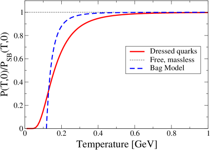
(a)

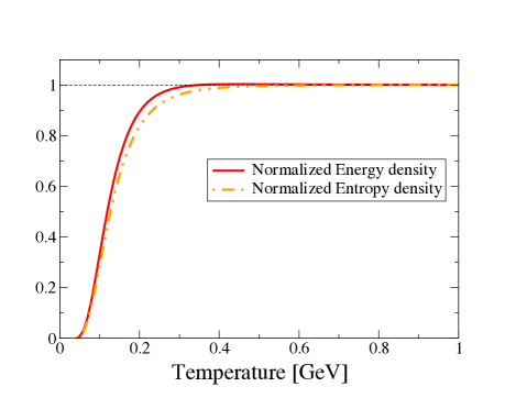
(b)

Figure 1: (a) Pressure as a function of temperature for $\mu=0$, normalized by the free gas limit (49) for nonlocal quarks and for the MIT bag model with bag constant $B=(0.145{\rm GeV})^{4}$. (b) Energy and entropy densities, normalized by the respective free gas limits.

In Fig. (1a), we show the pressure as a function of the temperature at zero chemical potential. We normalize the result by the pressure of free, massless fermions,

$$P_{SB}(T,\mu)=N_{c}N_{f}\left[\frac{7\pi^{2}T^{4}}{180}+\frac{\mu^{2}T^{2}}{6}+\frac{\mu^{4}}{12\pi^{2}}\right],$$ (49)

evaluated at $\mu=0$. For comparison, we also display the pressure of massless quarks subject to a constant negative bag pressure $p_{Bag}=-B=-(0.145{\rm GeV})^{4}$.

A smooth but fast rise of the pressure as temperature increases is observed, indicating a drastic change in the number of thermal degrees of freedom between low- and high-temperature systems. A similar behavior is seen for the thermal crossover in lattice QCD simulations. In contrast to the bag model, our model is capable of describing the whole range of temperatures, with no negative pressures attained at low temperatures. This corroborates the thermodynamical stability of the model and its consistency. The associated energy and entropy densities at $\mu=0$, normalized by their respective free gas limits, present a similar behavior as functions of temperature, as can be seen in Fig. (1b).

Another thermodynamic observable of interest is the (normalized) trace anomaly or “interaction measure”

$$\Delta(T,\mu)=\frac{E-3P}{T^{4}}.$$ (50)

It corresponds to the deviation from the tracelessness of a conformal energy-momentum tensor (normalized by $T^{4}$), or, in other words, it measures how different the nonlocal quark system behaves with respect to an ideal gas of massless quarks. The trace anomaly for the nonlocal quarks, plotted in Fig. (2a), is clearly different from the bag model result and shows a peak around $T\simeq 0.15$GeV. This suggests a smooth transition between two quasi conformal phases at low and high temperatures. However, in such a transition, the sound velocity squared,

$$c_{s}^{2}=\frac{\partial P}{\partial E},$$ (51)

typically presents a minimum around the transition temperature and this is not seen in (2b).

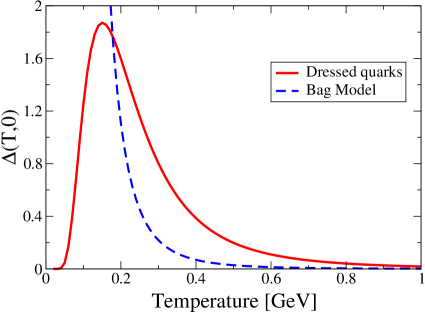
(a)

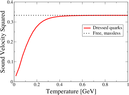
(b)

Figure 2: (a) Trace anomaly as a function of temperature for zero chemical potential, normalized by $T^{4}$. A clear distinction from the bag model result is seen. (b) Sound velocity squared as a function of temperature.

Due to asymptotic freedom and chiral symmetry restoration, encoded in the $p\rightarrow\infty$ limit of the mass function (8), it is expected that the system approaches the limit of free, massless quarks as temperature increases. This is indeed seen from our results for all the thermodynamic quantities we calculated. On the other hand, the non-trivial interactions included in our model via the nonlocal background show up in the results for intermediate temperatures. There is a clear change of behavior of all thermodynamic quantities at $T\simeq 0.15$GeV, the typical temperature scale of the chiral or deconfined phase crossover. In particular, the trace anomaly shows a peak precisely at this temperature, with a steep rise from zero as observed e.g. in lattice QCD simulations and in contrast to QM models. It is interesting that the inclusion of a well-chosen Polyakov-loop potential (fitted to thermal lattice data) may provide exactly this steep rise in the trace anomaly at low temperatures, which is absent in pure chiral models Schaefer:2009ui . In this sense, and for this particular observable, our nontrivial background – encoded in the nonlocal quark propagator fitted to zero-temperature lattice results – seems to play a similar role as the Polyakov-loop potential, further suggesting its connection to confinement and nonperturbative physics.

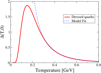
Figure 3: High-temperature fit (dotted line) of the trace anomaly as a function of temperature for zero chemical potential, normalized by $T^{4}$. The solid, red line represent our model results.

In order to further understand the physics contained in our result for temperatures above the peak, we display in Fig.3 a fit of the trace anomaly in the temperature interval $T\in[300,800]$ MeV in the following form:

$$[\Delta(T,\mu=0)]_{\rm high\,T}=a+\frac{b}{T^{2}}+\frac{c}{T^{4}}\,,$$ (52)

with $a=-0.069$, $b=0.062$ GeV² and $c=0.0016$ GeV⁴, with the $O(T^{-2})$ term dominant over the $O(T^{-4})$ one in this range.

A fit of the form (52) was also performed for lattice data in Ref.Cheng:2007jq . There they observe a similar hierarchy of contributions, with $b_{\rm latt}\sim 0.1$ GeV² and $c_{\rm latt}\sim 0.02$ GeV⁴. We note, however, that direct comparison of these results should be taken with care, since the system from Ref.Cheng:2007jq is (2+1)-flavour full QCD, while our model describes only heavier-than-physical degenerate up and down quarks, with gluons not explicitly included (their influence appears only in the nonperturbative quark dressing). It is nevertheless encouraging that the same structure and hierarchy of contributions is found in our confining quark model, in contrast to the bag model or a free massive quark system, as will be detailed below.

The three terms in the fit (52) may be associated with different physical contributions. The constant $a$ is related to a logarithmic dependence in the pressure, i.e. $\sim\log T$, that could in principle be mapped to the perturbative result (including the running coupling), if the temperature is high enough. The parameter $c$ is originated by a constant pressure, which is negative for positive $c$. This is exactly the type of contribution included in an ad hoc manner in a bag model to mimic confinement, and that appears here as a natural consequence of the nontrivial background considered. An estimate of the bag constant predicted in the high-temperature region of our model can then be obtained from $c=4B$, yielding $B\sim(141\,{\rm MeV})^{4}$ which nicely falls in the ballpark of the values adopted in the literature of QCD models.

The $O(T^{-2})$ term in the trace anomaly, however, is usually absent or very small in a naïve bag model. The smallness of this term is directly related to the lightness of up and down quarks. Indeed, a massive bag model has a pressure of the form KapustaGale :

$$P_{\rm bag}=\#_{0}T^{4}-\#_{1}m^{2}T^{2}-B\,,$$ (53)

where $m$ is the current quark mass. The respective trace anomaly is $T^{4}\Delta_{\rm bag}=4B+\#_{2}m^{2}T^{2}$. Taking $m=14$ MeV, the coefficient of $T^{-2}$ is $\sim 10^{-4}$ GeV², three orders of magnitude below the value obtained in this fit of our model and also in lattice QCD. It becomes clear that the presence of a dominant $O(T^{-2})$ contribution may be linked to the generation of a large mass scale in the nonperturbative quark sector, as the $M_{3}$ parameter in our model. It is worthwhile noting that even a bag model that considers effective quark masses large enough to give the desired $T^{-2}$ contribution would fail to reproduce lattice data for $T<300$ MeV, due to the nonperturbative peak structure that is developed for lower temperatures.

IV.2 Cold and dense confined quarks

Let us now turn our attention to the $T\rightarrow 0$ case and study some thermodynamic quantities as functions of the chemical potential $\mu$. This regime of QCD presents a severe Sign Problem which hinders the application of Montecarlo simulations, so that model predictions are extremely valuable tools to explore this region of the phase diagram.

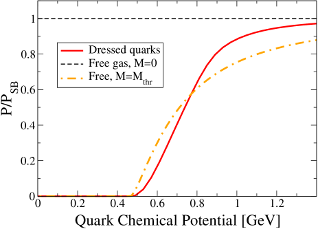
(a)

Figure 4: Pressure as a function of the chemical potential for $T=0$, normalized by the free gas limit $P_{SB}(0,\mu)=N_{c}N_{f}\mu^{4}/12\pi^{2}$. The massless (dotted) and massive (dot-dashed) free gas results are plotted for comparison. We use $M_{thr}=467$ MeV.

In Fig. (4), we show the pressure as a function of the chemical potential, at zero temperature. We compare the pressure from the model with that of local massive quarks of mass $M_{thr}=0.467$ GeV, both normalized to the pressure of massless quarks. The choice of the mass $M_{thr}$ is the one that provides a pressure that better compares to our model results in order to make explicit the differences and the specific features that are exclusive to the confining quark model here studied.

Since the system is at zero temperature there is no thermal energy to excite particles at low densities, yielding a vanishing thermodynamical response. As already observed in the thermal case, the results are fully stable and consistent with general physical expectations for a cold and dense system. In particular, the pressure vanishes for chemical potentials up to some value $\mu\simeq M_{thr}=0.467\,$GeV, which is consistent with a dynamically generated scale and not directly connected to any specific mass parameter of the model. Starting at this point, the pressure smoothly rises until reaching the limiting pressure of local quarks for high chemical potentials. It is not surprising that the massless limit is attained at large chemical potentials, given the $\mu$-dependence of the momentum-dependent mass function in Eq. (16).

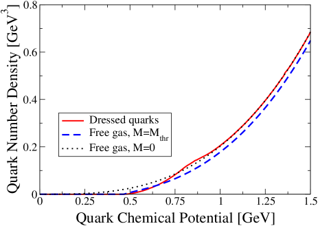
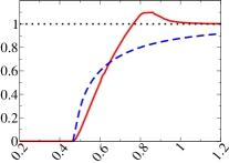
(a)

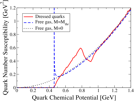
(b)

Figure 5: (a) Quark density as a function of chemical potential $\mu$ (with the results normalized by the free massless case in the detail) and (b) quark number susceptibility at $T\rightarrow 0$. Notice the approach to the free, massless limit $\chi_{SB}=N_{c}N_{f}\mu^{2}/\pi^{2}$ as $\mu\rightarrow\infty$. There is a clear threshold at a scale $\mu\approx M_{thr}=0.467$GeV.

Besides the pressure, two other relevant observables that can be calculated are the quark density (47), and the quark number susceptibility (48), as shown in Figs. (5a) and (5b). The behavior of these observables is reasonably smooth and interpolates between that of free massless and massive quarks. The quark susceptibility is a non-monotonic function of the chemical potential, having an oscillation inside the window $0.8\,{\rm GeV}\lesssim\mu\lesssim 1\,$GeV, resembling the result for the massive gas of free quarks, but with a smoothened behavior.

Even though it is not strictly proven that a first-order phase transition occurs in cold and dense QCD, it has been predicted in several low-energy QCD models. However, no sharp, first-order transition is observed in our predictions. The massive parameters in our model, $M_{3}$ and $m$ are fixed by zero-temperature, zero-$\mu$ lattice data for the quark propagator. They do not depend on temperature nor chemical potential. A crossover may be reasonably described, but a first-order phase transition needs symmetry changes that, we believe, will only be attained by $T-$ and $\mu-$dependent parameters or condensates, such as $M_{3}(T,\mu)$. Indeed, $M_{3}$ can be seen as a nonlocal order parameter for chiral symmetry breaking Dudal:2013vha and its $T,\mu$ dependence will thus play a significant role in the chiral phase transition.

IV.3 Results for $T\neq 0$ and $\mu\neq 0$

In this subsection, we consider a thermal system with an imbalance between the number of fermions and anti-fermions, given by a finite $\mu$. In Figs. (6a) and (6b), pressure and quark number density, respectively, are shown as functions of chemical potential for different values of temperature.

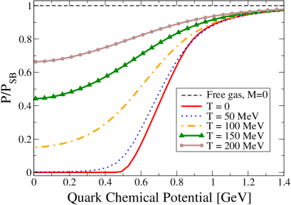
(a)

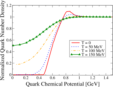
(b)

Figure 6: (a) Pressure and (b) quark number density (normalized by the free massless gas result) are plotted as functions of the chemical potential $\mu$ for temperature $T=\{0\textrm{ (bottom)},50,100,150,200\textrm{ (top)}\}$ MeV.

These results further support the physical consistency of our model and the absence of thermodynamical instabilities. Moreover, we see that, as temperature increases, more thermal energy becomes available, exciting particles even at lower chemical potentials, as expected. Even though we do not see a first-order phase transition at low temperatures, as discussed above, we do observe two qualitative features generally seen in QCD models: (i) a smoothening of the transition as temperature increases and (ii) a shift of the inflection point of the curve to lower values of $\mu$.

V Summary and discussion

In this paper, we made a first exploratory study of the thermodynamics of a softly BRST broken quark model. A soft breaking of the BRST symmetry could in principle be present in the infrared regime of QCD without affecting any ultraviolet (perturbative) predictions. In this case, the BRST breaking may be intimately related to other nonperturbative phenomena, such as confinement and chiral symmetry breaking, representing a complementary way to study these issues. Evidence for this breaking has been recently found on lattice studies in the gluon sector Cucchieri:2014via . It also provides an argument for the absence of asymptotic quarks in the spectrum as well as a good analytical description of nonperturbative quark propagators as compared to lattice.

We adopt the tree-level approximation in our model, so that no explicit quark-gluon interactions are present. Nevertheless, gluon dynamics is encoded in the nontrivial BRST-breaking background in the form of a nonlocal quark propagator. The model reduces itself to a free quark model in the high energy limit, corresponding to the fermionic sector of Quantum Chromodynamics, and yields an infrared dynamics compatible with the available lattice data for quark propagators. Within this model, as in other nonperturbative approaches to QCD, confinement is encoded in the presence of complex poles in the momentum-space quark propagator, i.e., complex masses. The quark propagator adopted here has been explicitly shown to violate reflection positivity, being compatible with the absence of asymptotic quark physical states.

Despite the presence of the nontrivial BRST-breaking background, the theory is quadratic in the quark fields. Therefore, the grand canonical partition function of the model could be calculated exactly at finite temperature and chemical potential. This allowed a computation of several thermodynamic quantities, as shown in the previous section. It is important to note that this model does not lead to thermodynamic instabilities, in spite of the presence of complex poles in propagator. We believe that the presence of three poles (one of them real) in the propagator of our model is a crucial feature to guarantee the consistency of the thermodynamic predictions, since quark models with pair of complex-conjugated poles alone have displayed unphysical macroscopic behavior Benic:2012ec .

Besides presenting a consistent thermodynamic behavior – free of instabilities –, the model displays nontrivial physical results, even at tree level. At finite temperature and vanishing chemical potential, one sees a nontrivial behavior of thermodynamic observables, which clearly differ from the case of free quarks at low and intermediate temperatures, while recovering the standard free case at high temperatures. This can be seen as an effect of the momentum-dependent mass function, which is in turn a manifestation of the soft BRST breaking. It is interesting to notice that there is a clear rise in the pressure, as well as a peak in the trace anomaly, at around $T\sim 0.15\,$GeV, the temperature scale of the deconfinement and chiral restoration crossovers. In spite of this, one may not associate this change of behavior with a phase transition, as other signatures are not present, as e.g. a dip in the sound velocity.

The model also allowed us to access the region of finite chemical potential at arbitrary temperatures, including a well-defined $T\rightarrow 0$ limit. The finite density thermodynamics was also shown to contain nontrivial features, differing from an ideal quark gas picture. The system has no excitations until a threshold chemical potential $\mu\sim M_{thr}=0.467\,$GeV is achieved, so that the Silver-Blaze property Muroya:2003qs ; Cohen:2004qp is satisfied. For larger chemical potentials, the limit of massless free quarks is approached. In spite of the clear excitation threshold $M_{thr}$, it is probably not correct to interpret the system as a gas of constituent quarks of mass $M_{thr}$, as can be seen, e.g., from the comparison of the respective pressures in Fig. (4). It seems more appropriate to resort to an interpretation in terms of an ensemble of resonances with different masses. This idea seems to be supported by the momentum and chemical potential dependence of the mass function (16). As the chemical potential is increased, more phase space is made available for excitations with different momenta. Given that the mass depends on both $\mu$ and ${\bf p}$, these newly available states have different masses as those present before. A similar interpretation seems to be actually possible for any $T$ or $\mu$.

Of course, further improvements and perspectives are possible and planned. Our results for the equation of state at large densities and low temperatures may in principle be further developed to investigate whether a physical compact star with a quark matter core could be created in this model. The explicit inclusion of interactions on top of the already nontrivial nonperturbative background may be implemented through different couplings, such as four-fermion or quark-gluon vertices, to be added perturbatively. Moreover, in order to explicitly compute the Polyakov loop in our model one could compute its effective potential in the background field formalism (for recent pure glue studies, see Refs. Canfora:2015yia ; Reinosa:2014zta ; Reinosa:2014ooa and Ref.Reinosa:2015oua for the case with heavy quarks). This way one may understand further the significant change of thermodynamic quantities observed here in terms of the approximate order parameter for the deconfinement phase transition.

Appendix A Fermion effective action at finite $T$ and $\mu$

A.1 Model hamiltonian

The first step to calculate the grand partition function is to determine the hamiltonian density of the theory. It can be obtained from the lagrangian density in Minkowski space

$${\cal L}={\cal L}_{Dirac}+{\cal L}_{\xi\lambda}+{\cal L}_{M},$$ (54)

where, omitting spinor, color, and flavor indices,

$${\cal L}_{Dirac}=\bar{\psi}\,i\gamma^{\mu}\partial_{\mu}\psi-m_{0}\bar{\psi}\psi,$$ (55)

and

$${\cal L}_{\xi\lambda}=\bar{\xi}(-\partial^{2}+m^{2})\lambda+\bar{\lambda}(-\partial^{2}+m^{2})\xi+\bar{\eta}(-\partial^{2}+m^{2})\theta-\bar{\theta}(-\partial^{2}+m^{2})\eta,$$ (56)

and

$${\cal L}_{M}=M_{1}^{2}(\bar{\xi}\psi+\bar{\psi}\xi)-M_{2}(\bar{\lambda}\psi+\bar{\psi}\lambda)$$ (57)

The hamiltonian is the Legendre transformation of the lagrangian with respect to the generalized velocity, that is

$${\cal H}=\sum_{i}\Pi_{\phi_{i}}(\partial_{0}\phi_{i})-{\cal L},$$ (58)

where $\Pi_{\phi_{i}}$ is the momentum conjugated to the field $\phi_{i}$. The field momenta are defined as Swanson:book

$$\Pi_{\phi_{i}}=\frac{\partial{\cal L}}{\partial(\partial_{0}\phi_{i})}\;\;\;\;\mbox{for bosonic fields}$$ (59)

or

$$\Pi_{\phi_{i}}=-\frac{\partial{\cal L}}{\partial(\partial_{0}\phi_{i})}\;\;\;\;\mbox{for fermionic fields}$$ (60)

After adding a total derivative to ${\cal L}_{\xi\lambda}$, one straightforwardly finds the following set of field momenta

$$\begin{array}[]{c|c|c|c}\Pi_{\xi}=\partial_{0}\bar{\lambda}&\Pi_{\bar{\xi}}=-\partial_{0}\lambda&\Pi_{\lambda}=\partial_{0}\bar{\xi}&\Pi_{\bar{\lambda}}=-\partial_{0}\xi\\ \hline\cr\Pi_{\theta}=\partial_{0}\bar{\eta}&\Pi_{\bar{\theta}}=-\partial_{0}\eta&\Pi_{\eta}=-\partial_{0}\bar{\theta}&\Pi_{\bar{\eta}}=\partial_{0}\theta\end{array}$$ (61)

It is important to notice that due to the first-order nature of the Dirac equation, the quark fields $\psi$ and $\bar{\psi}$ are actually such that $i\bar{\psi}\gamma_{0}$ is the momentum conjugated to the field $\psi$, i.e.,

$$\Pi_{\psi}=i\bar{\psi}\gamma_{0}$$ (62)

Putting all pieces together, the hamiltonian density can be written as

$${\cal H}={\cal H}_{Dirac}+{\cal H}_{\xi\lambda}+{\cal H}_{M},$$ (63)

where

$${\cal H}_{Dirac}[\Pi_{\psi},\psi]=-\Pi_{\psi}\gamma_{0}\vec{\gamma}\cdot\nabla\psi-im_{0}\Pi_{\psi}\gamma_{0}\psi,$$ (64)

and

$${\cal H}_{\xi\lambda}= \Pi_{\xi}\partial_{0}\xi+\Pi_{\bar{\xi}}\partial_{0}\bar{\xi}+\Pi_{\lambda}\partial_{0}\lambda+\Pi_{\bar{\lambda}}\partial_{0}\bar{\lambda}+\Pi_{\theta}\partial_{0}\theta+\Pi_{\bar{\theta}}\partial_{0}\bar{\theta}+\Pi_{\eta}\partial_{0}\eta+\Pi_{\bar{\eta}}\partial_{0}\bar{\eta}-{\cal L}_{\xi\lambda}$$ (65)

$$=\Pi_{\bar{\xi}}\Pi_{\lambda}+\Pi_{\bar{\lambda}}\Pi_{\xi}-\Pi_{\bar{\theta}}\Pi_{\eta}+\Pi_{\bar{\eta}}\Pi_{\theta}-(\nabla\bar{\xi})\cdot(\nabla\lambda)-(\nabla\bar{\lambda})\cdot(\nabla\xi)-(\nabla\bar{\eta})\cdot(\nabla\theta)+(\nabla\bar{\theta})\cdot(\nabla\eta)-$$

$$-m^{2}(\bar{\xi}\lambda+\bar{\lambda}\xi+\bar{\eta}\theta-\bar{\theta}\eta),$$

and

$${\cal H}_{M}=-{\cal L}_{M}=-M_{1}^{2}(\bar{\xi}\psi+\bar{\psi}\xi)+M_{2}(\bar{\lambda}\psi+\bar{\psi}\lambda).$$ (66)

A.2 Noether current

In the grand canonical ensemble the average charge of the system is kept constant. This constraint can be imposed by the replacement ${\cal H}\rightarrow{\cal H}-\mu j_{0}$, where $j_{0}$ is the charge density and $\mu$ the corresponding chemical potential. From a field theoretical point of view, such a charge density is consistently defined as the time component of the Noether current associated with a global $U(1)$ transformation. Let us now define one such transformation for the theory at hand and find the associated Noether charge.

In order to define the quark number, we first notice that the action is symmetric under the $U(1)$ transformation

$$\psi\rightarrow e^{-i\alpha}\psi,\;\;\;\;\bar{\psi}\rightarrow e^{i\alpha}\bar{\psi}$$

$$\xi\rightarrow e^{-i\alpha}\xi,\;\;\;\;\bar{\xi}\rightarrow e^{i\alpha}\bar{\xi}$$

$$\lambda\rightarrow e^{-i\alpha}\lambda,\;\;\;\;\bar{\lambda}\rightarrow e^{i\alpha}\bar{\lambda}$$

$$\eta\rightarrow e^{-i\alpha}\eta,\;\;\;\;\bar{\eta}\rightarrow e^{i\alpha}\bar{\eta}$$

$$\theta\rightarrow e^{-i\alpha}\theta,\;\;\;\;\bar{\theta}\rightarrow e^{i\alpha}\bar{\theta}$$ (67)

The corresponding Noether current is

$$j^{\mu}=\sum_{i}\Delta\phi_{i}\frac{\partial{\cal L}}{\partial(\partial_{\mu}\phi_{i})}$$ (68)

and the charge density is

$$j_{0}=\sum_{i}\Delta\phi_{i}\frac{\partial{\cal L}}{\partial(\partial_{0}\phi_{i})}=\sum_{b}\Delta\phi_{b}\,\Pi_{\phi_{b}}-\sum_{f}\Delta\phi_{f}\,\Pi_{\phi_{f}},$$ (69)

where we recalled the definitions of field momenta for bosons (59) and fermions (60). The explicit expression for the charge density in terms of fields and field momenta is

$$j_{0}=i\psi\Pi_{\psi}+i\xi\Pi_{\xi}-i\bar{\xi}\Pi_{\bar{\xi}}+i\lambda\Pi_{\lambda}-i\bar{\lambda}\Pi_{\bar{\lambda}}-i\theta\Pi_{\theta}+i\bar{\theta}\Pi_{\bar{\theta}}-i\eta\Pi_{\eta}+i\bar{\eta}\Pi_{\bar{\eta}}.$$ (70)

A.3 Quark in-medium effective action

In the functional integral formalism, the partition function is written as

$$Z(T,\mu)= {\rm Tr}\exp\left(-\beta\hat{H}+\beta\mu\hat{Q}\right)$$

$$= \int[D\Pi_{\psi}][D\psi][D\xi][D\Pi_{\xi}][D\bar{\xi}][D\Pi_{\bar{\xi}}][D\lambda][D\Pi_{\lambda}][D\bar{\lambda}][D\Pi_{\bar{\lambda}}][D\eta][D\Pi_{\eta}][D\bar{\eta}][D\Pi_{\bar{\eta}}][D\theta][D\Pi_{\theta}][D\bar{\theta}][D\Pi_{\bar{\theta}}]$$ (71)

$$\times\exp\left[\int_{0}^{\beta}d^{4}x\left(\sum_{i}i\Pi_{i}(\partial_{4}\phi_{i})-{\cal H}+\mu j_{4}\right)\right],$$

where now the fields have been analytically continued to imaginary time according to $x_{0}\rightarrow x_{4}=ix_{0}$. The constraint of finite temperature is imposed on the system by taking the time direction compact, i.e., $0\leq x_{4}\leq\beta\equiv 1/T$. This is expressed in the integration symbol

$$\int_{0}^{\beta}\,d^{4}x\,(\cdots)\equiv\int_{0}^{\beta}\,dx_{4}\int\,d^{3}x\,(\cdots).$$ (72)

Notice that one must start from the expression (A.3), where integration over field momenta must still be made. As is well known from the study of a complex scalar field (see, e.g., KapustaGale ), the field momentum integration in the presence of a chemical potential does not simply lead to the lagrangian plus a $\mu j_{4}$ term. Rather, the result of including a chemical potential is typically to shift the time derivative as $\partial_{4}\rightarrow(\partial_{4}-\mu)$.

The integrand of the exponent of (A.3) is

$$I:= \sum_{k}i\Pi_{k}\dot{\phi}_{k}-{\cal H}+\mu j_{4}$$

$$= i\Pi_{\psi}\dot{\psi}+i\Pi_{\xi}\dot{\xi}+i\Pi_{\bar{\xi}}\dot{\bar{\xi}}+i\Pi_{\lambda}\dot{\lambda}+i\Pi_{\bar{\lambda}}\dot{\bar{\lambda}}+i\Pi_{\theta}\dot{\theta}+i\Pi_{\bar{\theta}}\dot{\bar{\theta}}+i\Pi_{\eta}\dot{\eta}+i\Pi_{\bar{\eta}}\dot{\bar{\eta}}+$$

$$+\Pi_{\psi}\gamma_{0}\vec{\gamma}\cdot\nabla\psi+im_{0}\Pi_{\psi}\gamma_{0}\psi-\Pi_{\bar{\xi}}\Pi_{\lambda}-\Pi_{\bar{\lambda}}\Pi_{\xi}+\Pi_{\bar{\theta}}\Pi_{\eta}-\Pi_{\bar{\eta}}\Pi_{\theta}+$$

$$+(\nabla\bar{\xi})\cdot(\nabla\lambda)+(\nabla\bar{\lambda})\cdot(\nabla\xi)+(\nabla\bar{\eta})\cdot(\nabla\theta)-(\nabla\bar{\theta})\cdot(\nabla\eta)+$$

$$+m^{2}(\bar{\xi}\lambda+\bar{\lambda}\xi+\bar{\eta}\theta-\bar{\theta}\eta)+M_{1}^{2}(\bar{\xi}\psi+\bar{\psi}\xi)-M_{2}(\bar{\lambda}\psi+\bar{\psi}\lambda)+$$

$$-i\mu\Pi_{\psi}\psi-i\mu\Pi_{\xi}\xi+i\mu\Pi_{\bar{\xi}}\bar{\xi}-i\mu\Pi_{\lambda}\lambda+i\mu\Pi_{\bar{\lambda}}\bar{\lambda}-$$

$$-i\mu\theta\Pi_{\theta}+i\mu\bar{\theta}\Pi_{\bar{\theta}}-i\mu\eta\Pi_{\eta}+i\mu\bar{\eta}\Pi_{\bar{\eta}}$$

$$= i\Pi_{\psi}\left(\dot{\psi}-\mu\psi-i\gamma_{0}\vec{\gamma}\cdot\nabla\psi+m_{0}\gamma_{0}\psi\right)+i\Pi_{\bar{\xi}}(\dot{\bar{\xi}}+\mu\bar{\xi})+i\Pi_{\lambda}(\dot{\lambda}-\mu\lambda)+$$ (73)

$$+i\Pi_{\bar{\lambda}}(\dot{\bar{\lambda}}+\mu\bar{\lambda})+i\Pi_{\xi}(\dot{\xi}-\mu\xi)+i\Pi_{\bar{\theta}}(\dot{\bar{\theta}}+\mu\bar{\theta})+i\Pi_{\eta}(\dot{\eta}-\mu\eta)+$$

$$+i\Pi_{\bar{\eta}}(\dot{\bar{\eta}}+\mu\bar{\eta})+i\Pi_{\theta}(\dot{\theta}-\mu\theta)-\Pi_{\bar{\xi}}\Pi_{\lambda}-\Pi_{\bar{\lambda}}\Pi_{\xi}+\Pi_{\bar{\theta}}\Pi_{\eta}-\Pi_{\bar{\eta}}\Pi_{\theta}+$$

$$+(\nabla\bar{\xi})\cdot(\nabla\lambda)+(\nabla\bar{\lambda})\cdot(\nabla\xi)+(\nabla\bar{\eta})\cdot(\nabla\theta)-(\nabla\bar{\theta})\cdot(\nabla\eta)+$$

$$+m^{2}(\bar{\xi}\lambda+\bar{\lambda}\xi+\bar{\eta}\theta-\bar{\theta}\eta)+M_{1}^{2}(\bar{\xi}\psi+\bar{\psi}\xi)-M_{2}(\bar{\lambda}\psi+\bar{\psi}\lambda)$$

where we used the notation $(\dot{\phi}_{k}\equiv\partial_{4}\phi_{k})$.

Note that we can separetely integrate the bosonic and the fermionic auxiliary fields. As a result, we shall find an effective action for the fermion fields. Interestingly enough, we find a similar result as compared to the vacuum nonlocal action, Eq. (6), the only difference being the replacement $\partial_{4}^{2}\rightarrow-(i\omega_{n}+\mu)^{2}$. We now demonstrate this result, while we leave the integral in the quark field $\psi$ to the main text.

Let us first consider the anticommuting auxiliary fields $(\xi,\bar{\xi},\lambda,\bar{\lambda})$. The relevant part of the integrand for the field momentum integral is

$$I_{\Pi_{f}}:= -\Pi_{\bar{\xi}}\Pi_{\lambda}+i\Pi_{\bar{\xi}}(\dot{\bar{\xi}}+\mu\bar{\xi})+i\Pi_{\lambda}(\dot{\lambda}-\mu\lambda)-\Pi_{\bar{\lambda}}\Pi_{\xi}+i\Pi_{\bar{\lambda}}(\dot{\bar{\lambda}}+\mu\bar{\lambda})+i\Pi_{\xi}(\dot{\xi}-\mu\xi)$$

$$= -\left[\Pi_{\bar{\xi}}+i\left(\dot{\lambda}-\mu\lambda\right)\right]\left[\Pi_{\lambda}-i\left(\dot{\bar{\xi}}+\mu\bar{\xi}\right)\right]-\left[\Pi_{\bar{\lambda}}+i\left(\dot{\xi}-\mu\xi\right)\right]\left[\Pi_{\xi}-i\left(\dot{\bar{\lambda}}+\mu\bar{\lambda}\right)\right]-$$ (74)

$$-\left(\dot{\bar{\xi}}+\mu\bar{\xi}\right)\left(\dot{\lambda}-\mu\lambda\right)-\left(\dot{\bar{\lambda}}+\mu\bar{\lambda}\right)\left(\dot{\xi}-\mu\xi\right)$$

Notice that the field variables and momenta above are Grassmann variables. Once this expression is under a functional integral, we may shift the momenta in $I_{f}$ without changing the integral, so that

$$Z_{\Pi_{f}}:=\int[D\Pi_{\xi}][D\Pi_{\bar{\xi}}][D\Pi_{\lambda}][D\Pi_{\bar{\lambda}}]e^{\int_{0}^{\beta}\,d^{4}x\,I_{f}}$$ (75)

$$=e^{-\int_{0}^{\beta}\,d^{4}x\,\left[\left(\dot{\bar{\xi}}+\mu\bar{\xi}\right)\left(\dot{\lambda}-\mu\lambda\right)+\left(\dot{\bar{\lambda}}+\mu\bar{\lambda}\right)\left(\dot{\xi}-\mu\xi\right)\right]}\int[D\Pi_{\xi}][D\Pi_{\bar{\xi}}][D\Pi_{\lambda}][D\Pi_{\bar{\lambda}}]e^{-\int_{0}^{\beta}\,d^{4}x\,\left(\Pi_{\bar{\xi}}\Pi_{\lambda}+\Pi_{\bar{\lambda}}\Pi_{\xi}\right)}$$

$$=e^{-\int_{0}^{\beta}\,d^{4}x\,\left[\left(\dot{\bar{\xi}}+\mu\bar{\xi}\right)\left(\dot{\lambda}-\mu\lambda\right)+\left(\dot{\bar{\lambda}}+\mu\bar{\lambda}\right)\left(\dot{\xi}-\mu\xi\right)\right]}$$

Let us now compute the momentum integral of the bosonic auxiliary fields. The relevant integrand is

$$I_{\Pi_{b}}= \Pi_{\bar{\theta}}\Pi_{\eta}+i\Pi_{\bar{\theta}}\left(\dot{\bar{\theta}}+\mu\bar{\theta}\right)+i\Pi_{\eta}\left(\dot{\eta}-\mu\eta\right)-\Pi_{\bar{\eta}}\Pi_{\theta}+i\Pi_{\bar{\eta}}\left(\dot{\bar{\eta}}+\mu\bar{\eta}\right)+i\Pi_{\theta}\left(\dot{\theta}-\mu\theta\right)$$

$$= \left[\Pi_{\bar{\theta}}+i(\dot{\eta}-\mu\eta)\right]\left[\Pi_{\eta}+i\left(\dot{\bar{\theta}}+\mu\bar{\theta}\right)\right]-\left[\Pi_{\bar{\eta}}-i(\dot{\theta}-\mu\theta)\right]\left[\Pi_{\theta}-i\left(\dot{\bar{\eta}}+\mu\bar{\eta}\right)\right]+$$ (76)

$$+\left(\dot{\bar{\theta}}+\mu\bar{\theta}\right)\left(\dot{\eta}-\mu\eta\right)-\left(\dot{\bar{\eta}}+\mu\bar{\eta}\right)\left(\dot{\theta}-\mu\theta\right)$$

As in the fermionic case, for fixed field configurations, one is allowed to shift the field momenta by any arbitrary function without changing the functional integral. As a result,

$$Z_{\Pi_{b}}:= \int[D\Pi_{\eta}][D\Pi_{\bar{\eta}}][D\Pi_{\theta}][D\Pi_{\bar{\theta}}]e^{\int_{0}^{\beta}\,d^{4}x\,I_{b}}$$

$$= e^{\int_{0}^{\beta}\,d^{4}x\,\left[\left(\dot{\bar{\theta}}+\mu\bar{\theta}\right)\left(\dot{\eta}-\mu\eta\right)+\left(\dot{\bar{\eta}}+\mu\bar{\eta}\right)\left(\dot{\theta}-\mu\theta\right)\right]}\int[D\Pi_{\eta}][D\Pi_{\bar{\eta}}][D\Pi_{\theta}][D\Pi_{\bar{\theta}}]e^{\int_{0}^{\beta}\,d^{4}x\,\left[\Pi_{\bar{\theta}}\Pi_{\eta}+\Pi_{\bar{\eta}}\Pi_{\theta}\right]}$$

$$= e^{\int_{0}^{\beta}\,d^{4}x\,\left[\left(\dot{\bar{\theta}}+\mu\bar{\theta}\right)\left(\dot{\eta}-\mu\eta\right)-\left(\dot{\bar{\eta}}+\mu\bar{\eta}\right)\left(\dot{\theta}-\mu\theta\right)\right]}$$ (77)

In our next step, we integrate over the auxiliary boson fields $(\theta,\bar{\theta},\eta,\bar{\eta})$. The relevant integrand is

$$I_{b}:= \left(\dot{\bar{\theta}}+\mu\bar{\theta}\right)\left(\dot{\eta}-\mu\eta\right)-\left(\dot{\bar{\eta}}+\mu\bar{\eta}\right)\left(\dot{\theta}-\mu\theta\right)+(\nabla\bar{\eta})\cdot(\nabla\theta)-(\nabla\bar{\theta})\cdot(\nabla\eta)+m^{2}(\bar{\eta}\theta-\bar{\theta}\eta)$$

$$= \dot{\bar{\theta}}\dot{\eta}-\mu\dot{\bar{\theta}}\eta+\mu\bar{\theta}\dot{\eta}-\mu^{2}\bar{\theta}\eta+(\nabla\bar{\eta})\cdot(\nabla\theta)+m^{2}\bar{\eta}\theta--\left[\dot{\bar{\eta}}\dot{\theta}-\mu\dot{\bar{\eta}}\theta+\mu\bar{\eta}\dot{\theta}-\mu^{2}\bar{\theta}\eta+(\nabla\bar{\theta})\cdot(\nabla\eta)+m^{2}\bar{\theta}\eta\right]$$

$$\longrightarrow \bar{\theta}\left(-\partial_{0}^{2}+2\mu\partial_{0}-\mu^{2}-\nabla^{2}+m^{2}\right)\eta-\bar{\eta}\left(-\partial_{0}^{2}+2\mu\partial_{0}-\mu^{2}-\nabla^{2}+m^{2}\right)\theta$$ (78)

where, in the last step we added a total derivative to the integrand. The resulting functional integral is (aside from an infinite numerical constant)

$$\int[D\bar{\theta}][D\theta][D\bar{\eta}][D\eta]e^{\int_{0}^{\beta}\,d^{4}x\,I_{b}} = \det[-D^{2}+m^{2}]^{-\frac{1}{2}(4N_{c})}\det[D^{2}-m^{2}]^{-\frac{1}{2}(4N_{c})}$$ (79)

$$= \det[-D^{2}+m^{2}]^{-4N_{c}},$$

where we defined the operator $D^{2}:=(\partial_{4}-\mu)^{2}+\nabla^{2}$, which corresponds to $(i\omega_{n}+\mu)^{2}-{\bf p}^{2}$ in momentum space. At this point, it should be clear that the final result should be the same as the one at zero temperature (in euclidean space), with the replacement $p_{4}\rightarrow\omega_{n}-i\mu$. Let us continue our calculation in order to explicitly check that this is the case. The relevant integrand in the fermionic auxiliary fields is

$$I_{f}:= \left(\dot{\bar{\xi}}+\mu\bar{\xi}\right)\left(\dot{\lambda}-\mu\lambda\right)+\left(\dot{\bar{\lambda}}+\mu\bar{\lambda}\right)\left(\dot{\xi}-\mu\xi\right)+(\nabla\bar{\xi})\cdot(\nabla\lambda)+(\nabla\bar{\lambda})\cdot(\nabla\xi)+m^{2}(\bar{\xi}\lambda+\bar{\lambda}\xi)+$$ (80)

$$+M_{1}^{2}(\bar{\xi}\psi+\bar{\psi}\xi)-M_{2}(\bar{\lambda}\psi+\bar{\psi}\lambda)$$

$$\rightarrow\;\bar{\xi}\left(-D^{2}+m^{2}\right)\lambda+\bar{\lambda}\left(-D^{2}+m^{2}\right)\xi+M_{1}^{2}(\bar{\xi}\psi+\bar{\psi}\xi)-M_{2}(\bar{\lambda}\psi+\bar{\psi}\lambda),$$

where we added a total derivative and used the definition of $D^{2}$ in the last step.

The resulting functional integral is again not altered if we add constant functions to the integrated fields. Once the $\psi$ field is kept fixed in the integration of $(\bar{\xi},\xi,\bar{\lambda},\lambda)$, we may freely make the shifts

$$\xi\;\longrightarrow\;\xi+M_{2}\Delta^{-1}\psi\;\;\;\;\;\;\;\;\;\;\;\bar{\xi}\;\longrightarrow\;\bar{\xi}+M_{2}\bar{\psi}\Delta^{-1}$$

$$\lambda\;\longrightarrow\;\lambda-M_{1}^{2}\Delta^{-1}\psi\;\;\;\;\;\;\;\;\;\;\;\bar{\lambda}\;\longrightarrow\;\bar{\lambda}-M_{1}^{2}\bar{\psi}\Delta^{-1}$$

where $\Delta:=-D^{2}+m^{2}$. It follows that

$$I_{f}= \left(\bar{\xi}+M_{2}\bar{\psi}\Delta^{-1}\right)\Delta\left(\lambda-M_{1}^{2}\Delta^{-1}\psi\right)+\left(\bar{\lambda}-M_{1}^{2}\bar{\psi}\Delta^{-1}\right)\Delta\left(\xi+M_{2}\Delta^{-1}\psi\right)+$$ (82)

$$+M_{1}^{2}\left(\bar{\xi}+M_{2}\bar{\psi}\Delta^{-1}\right)\psi+M_{1}^{2}\bar{\psi}\left(\xi+M_{2}\Delta^{-1}\psi\right)-M_{2}\left(\bar{\lambda}-M_{1}^{2}\bar{\psi}\Delta^{-1}\right)\psi-M_{2}\bar{\psi}\left(\lambda-M_{1}^{2}\Delta^{-1}\psi\right)$$

$$=\bar{\xi}\Delta\lambda+\bar{\lambda}\Delta\xi+2M_{1}^{2}M_{2}\bar{\psi}\Delta^{-1}\psi$$

The integral in the fermionic auxiliary fields is then

$$\int[D\bar{\xi}][D\xi][D\bar{\lambda}][D\lambda]e^{-\int_{0}^{\beta}\,d^{4}x\,I_{f}} = \det[\Delta]^{4N_{c}}e^{-\int_{0}^{\beta}\,d^{4}x\,2M_{1}^{2}M_{2}\bar{\psi}\left(\Delta^{-1}\right)\psi}$$ (83)

$$= \det[-D^{2}+m^{2}]^{4N_{c}}e^{-\int_{0}^{\beta}\,d^{4}x\,2M_{1}^{2}M_{2}\bar{\psi}\left(\frac{1}{-D^{2}+m^{2}}\right)\psi}$$

We now finally arrive at our expression for the partition function in terms of the quark fields only

$$Z(T,\mu)=\int[D\Pi_{\psi}][D\psi]\exp\left[\int_{0}^{\beta}\,d^{4}x\,i\Pi_{\psi}\gamma_{4}\left(\gamma_{4}(\partial_{4}-\mu)-i\vec{\gamma}\cdot\nabla+\hat{M}_{p}\right)\psi\right]$$ (84)

where the nonlocal mass operator is

$$\hat{M}_{p}=\frac{2M_{1}^{2}M_{2}}{-D^{2}+m^{2}}+m_{0}\rightarrow\frac{2M_{1}^{2}M_{2}}{-(i\omega_{n}+\mu)^{2}+{\bf p}^{2}+m^{2}}+m_{0}$$ (85)

Finally, after the change of variables $\Pi_{\psi}\rightarrow\bar{\psi}=-i\Pi_{\psi}\gamma_{4}$, the partition function can be written as

$$Z(T,\mu)=\int[D\bar{\psi}][D\psi]\exp\left[-\int_{0}^{\beta}\,d^{4}x\,{\cal L}_{nl}[\bar{\psi},\psi]\right]$$ (86)

where

$${\cal L}_{nl}[\bar{\psi},\psi]=\bar{\psi}\left[\gamma_{4}(\partial_{4}-\mu)-i\vec{\gamma}\cdot\nabla+\frac{2M_{1}^{2}M_{2}}{-D^{2}+m^{2}}+m_{0}\right]\psi$$ (87)

is the (nonlocal) quark effective lagrangian at finite temperature and chemical potential.

References

- (1) C. Becchi, A. Rouet and R. Stora, Annals Phys. 98, 287 (1976).
- (2) I. V. Tyutin, arXiv:0812.0580 [hep-th].
- (3) V. N. Gribov, Nucl. Phys. B 139, 1 (1978).
- (4) A. Cucchieri, D. Dudal, T. Mendes and N. Vandersickel, arXiv:1405.1547 [hep-lat].
- (5) A. Cucchieri and T. Mendes, Phys. Rev. Lett. 100, 241601 (2008) [arXiv:0712.3517 [hep-lat]].
- (6) A. Cucchieri and T. Mendes, Phys. Rev. D 78, 094503 (2008) [arXiv:0804.2371 [hep-lat]].
- (7) A. Cucchieri, D. Dudal, T. Mendes and N. Vandersickel, Phys. Rev. D 85, 094513 (2012) [arXiv:1111.2327 [hep-lat]].
- (8) M. E. Peskin and D. V. Schroeder, Reading, USA: Addison-Wesley (1995) 842 p.
- (9) S. Weinberg, Cambridge, UK: Univ. Pr. (1995) 609 p.
- (10) R. Alkofer and L. von Smekal, Phys. Rept. 353, 281 (2001) [hep-ph/0007355].
- (11) N. Brambilla, S. Eidelman, P. Foka, S. Gardner, A. S. Kronfeld, M. G. Alford, R. Alkofer and M. Butenschoen et al., Eur. Phys. J. C 74 (2014) 10, 2981 [arXiv:1404.3723 [hep-ph]].
- (12) A. C. Aguilar, D. Binosi and J. Papavassiliou, Phys. Rev. D 78, 025010 (2008) [arXiv:0802.1870 [hep-ph]].
- (13) D. Dudal, S. P. Sorella, N. Vandersickel and H. Verschelde, Phys. Rev. D 77, 071501 (2008) [arXiv:0711.4496 [hep-th]].
- (14) D. Dudal, J. A. Gracey, S. P. Sorella, N. Vandersickel and H. Verschelde, Phys. Rev. D 78, 065047 (2008) [arXiv:0806.4348 [hep-th]].
- (15) D. Dudal, S. P. Sorella and N. Vandersickel, Phys. Rev. D 84, 065039 (2011) [arXiv:1105.3371 [hep-th]].
- (16) A. Cucchieri and T. Mendes, PoS QCD -TNT09, 026 (2009) [arXiv:1001.2584 [hep-lat]].
- (17) V. G. Bornyakov, V. K. Mitrjushkin and R. N. Rogalyov, Phys. Rev. D 86, 114503 (2012) [arXiv:1112.4975 [hep-lat]].
- (18) D. Dudal, M. S. Guimaraes and S. P. Sorella, Phys. Rev. Lett. 106, 062003 (2011) [arXiv:1010.3638 [hep-th]].
- (19) D. Dudal, M. S. Guimaraes and S. P. Sorella, Phys. Lett. B 732, 247 (2014) [arXiv:1310.2016 [hep-ph]].
- (20) M. B. Parappilly, P. O. Bowman, U. M. Heller, D. B. Leinweber, A. G. Williams and J. B. Zhang, Phys. Rev. D 73, 054504 (2006) [hep-lat/0511007].
- (21) M. A. L. Capri, M. S. Guimaraes, I. F. Justo, L. F. Palhares and S. P. Sorella, Phys. Rev. D 90, no. 8, 085010 (2014) [arXiv:1408.3597 [hep-th]].
- (22) L. Baulieu and S. P. Sorella, Phys. Lett. B 671, 481 (2009) [arXiv:0808.1356 [hep-th]].
- (23) D. Dudal, S. P. Sorella, N. Vandersickel and H. Verschelde, Phys. Rev. D 79, 121701 (2009) [arXiv:0904.0641 [hep-th]].
- (24) S. P. Sorella, Phys. Rev. D 80, 025013 (2009) [arXiv:0905.1010 [hep-th]].
- (25) S. P. Sorella, J. Phys. A 44, 135403 (2011) [arXiv:1006.4500 [hep-th]].
- (26) M. A. L. Capri, A. J. Gomez, M. S. Guimaraes, V. E. R. Lemes, S. P. Sorella and D. G. Tedesco, Phys. Rev. D 82, 105019 (2010) [arXiv:1009.4135 [hep-th]].
- (27) D. Dudal and S. P. Sorella, Phys. Rev. D 86, 045005 (2012) [arXiv:1205.3934 [hep-th]].
- (28) A. Reshetnyak, Int. J. Mod. Phys. A 29, 1450184 (2014) [arXiv:1312.2092 [hep-th]].
- (29) L. Baulieu, M. A. L. Capri, A. J. Gomez, V. E. R. Lemes, R. F. Sobreiro and S. P. Sorella, Eur. Phys. J. C 66, 451 (2010) [arXiv:0901.3158 [hep-th]].
- (30) D. Dudal, M. S. Guimaraes, L. F. Palhares and S. P. Sorella, arXiv:1303.7134 [hep-ph].
- (31) Y. Nambu and G. Jona-Lasinio, Phys. Rev. 122, 345 (1961).
- (32) M. Gell-Mann and M. Levy, Nuovo Cim. 16, 705 (1960).
- (33) P. N. Meisinger and M. C. Ogilvie, Phys. Lett. B 379, 163 (1996) [hep-lat/9512011].
- (34) K. Fukushima, Phys. Lett. B 591, 277 (2004) [hep-ph/0310121].
- (35) E. Megias, E. Ruiz Arriola and L. L. Salcedo, Phys. Rev. D 74, 065005 (2006) [hep-ph/0412308].
- (36) C. Ratti, M. A. Thaler and W. Weise, Phys. Rev. D 73, 014019 (2006) [hep-ph/0506234].
- (37) B. J. Schaefer, J. M. Pawlowski and J. Wambach, Phys. Rev. D 76, 074023 (2007) [arXiv:0704.3234 [hep-ph]].
- (38) B. J. Schaefer, M. Wagner and J. Wambach, Phys. Rev. D 81, 074013 (2010) [arXiv:0910.5628 [hep-ph]].
- (39) K. Osterwalder and R. Schrader, Commun. Math. Phys. 31, 83 (1973); Commun. Math. Phys. 42, 281 (1975).
- (40) I. General, D. Gomez Dumm and N. N. Scoccola, Phys. Lett. B 506, 267 (2001) [hep-ph/0010034].
- (41) G. A. Contrera, M. Orsaria and N. N. Scoccola, Phys. Rev. D 82, 054026 (2010) [arXiv:1006.4639 [hep-ph]].
- (42) S. Benic, D. Blaschke and M. Buballa, Phys. Rev. D 86, 074002 (2012) [arXiv:1206.6582 [hep-ph]].
- (43) S. Benic, D. Blaschke, G. A. Contrera and D. Horvatic, Phys. Rev. D 89, 016007 (2014) [arXiv:1306.0588 [hep-ph]].
- (44) M. Loewe, F. Marquez and C. Villavicencio, arXiv:1409.0500 [hep-ph].
- (45) D. Zwanziger, Phys. Rev. Lett. 94, 182301 (2005) [hep-ph/0407103].
- (46) D. Zwanziger, Phys. Rev. D 76, 125014 (2007) [hep-ph/0610021].
- (47) K. Lichtenegger and D. Zwanziger, Phys. Rev. D 78, 034038 (2008) [arXiv:0805.3804 [hep-ph]].
- (48) K. Fukushima and N. Su, Phys. Rev. D 88, 076008 (2013) [arXiv:1304.8004 [hep-ph]].
- (49) H. Reinhardt and J. Heffner, Phys. Lett. B 718, 672 (2012) [arXiv:1210.1742 [hep-th]].
- (50) H. Reinhardt and J. Heffner, Phys. Rev. D 88, no. 4, 045024 (2013) [arXiv:1304.2980 [hep-th]].
- (51) M. Le Bellac, Thermal Field Theory. Cambridge Moonographs on Mathematical Physics (1996).
- (52) A. Maas, PoS FACESQCD , 033 (2010) [arXiv:1102.0901 [hep-lat]].
- (53) A. Maas, Eur. Phys. J. C 71, 1548 (2011) [arXiv:1007.0729 [hep-lat]].
- (54) S. Furui and H. Nakajima, Phys. Rev. D 73, 074503 (2006).
- (55) M. S. Bhagwat, M. A. Pichowsky, C. D. Roberts and P. C. Tandy, Phys. Rev. C 68, 015203 (2003) [nucl-th/0304003].
- (56) J. I. Kapusta and C. Gale, Finite-Temperature Field Theory: Principles and Applications. Second Edition. Cambridge Monographs on Mathematical Physics (2006).
- (57) M. Cheng et al., Phys. Rev. D 77, 014511 (2008) [arXiv:0710.0354 [hep-lat]].
- (58) F. E. Canfora, D. Dudal, I. F. Justo, P. Pais, L. Rosa and D. Vercauteren, arXiv:1505.02287 [hep-th].
- (59) U. Reinosa, J. Serreau, M. Tissier and N. Wschebor, Phys. Rev. D 91, 045035 (2015) [arXiv:1412.5672 [hep-th]].
- (60) U. Reinosa, J. Serreau, M. Tissier and N. Wschebor, Phys. Lett. B 742, 61 (2015) [arXiv:1407.6469 [hep-ph]].
- (61) U. Reinosa, J. Serreau and M. Tissier, Phys. Rev. D 92, 025021 (2015) [arXiv:1504.02916 [hep-th]].
- (62) S. Muroya, A. Nakamura, C. Nonaka and T. Takaishi, Prog. Theor. Phys. 110, 615 (2003) [hep-lat/0306031].
- (63) T. D. Cohen, In *Shifman, M. (ed.) et al.: From fields to strings, vol. 1* 101-120 [hep-ph/0405043].
- (64) M. Swanson, Path Integrals and Quantum Processes. Dover (1992).