Entropy production in quantum Yang-Mills mechanics in semi-classical approximation

Abstract

We discuss thermalization of isolated quantum systems by using the Husimi-Wehrl entropy evaluated in the semiclassical treatment. The Husimi-Wehrl entropy is the Wehrl entropy obtained by using the Husimi function for the phase space distribution. The time evolution of the Husimi function is given by smearing the Wigner function, whose time evolution is obtained in the semiclassical approximation. We show the efficiency and usefulness of this semiclassical treatment in describing entropy production of a couple of quantum mechanical systems, whose classical counter systems are known to be chaotic. We propose two methods to evaluate the time evolution of the Husimi-Wehrl entropy, the test-particle method and the two-step Monte-Carlo method. We demonstrate the characteristics of the two methods by numerical calculations, and show that the simultaneous application of the two methods ensures the reliability of the results of the Husimi-Wehrl entropy at a given time.

A56,A52,D31

1 Introduction

Thermalization process or entropy creation of isolated quantum systems is a long-standing issue, but not well understood problem. Relevant systems include the early universe where the transition from a vacuum state to a thermalized state occurs at the end of cosmic inflation, and the QCD matter created in the initial stage of relativistic heavy-ion collisions where thermal matter should be formed in a rather short time. It is known that both systems are well described in semiclassical approximation, and moreover a chaotic behavior of the classical limit may play some role in the entropy production. The present paper is concerned with the entropy production of an isolated quantum system for which the semiclassical approximation is valid and the classical counter part may show a chaotic behavior.

To describe entropy in a pure quantum system, one may of course adopt the von Neumann entropy vonNeumann as quantum mechanical entropy given by

$$S_{\mathrm{vN}}= -\mathrm{Tr}\left[\rho\log\rho\right]\ ,$$ (1)

where $\rho$ is the density matrix. For a pure state, however, $\rho$ is idempotent, $\rho^{2}=\rho$, implying that the eigen value of $\rho$ is 0 or 1, and the von Neumann entropy is zero. Even if we start from a mixed state, the time evolution described by a unitary operator will never lead to entropy growth. On the other hand, the entropy production in a rarefied gas composed of classical or quantum mechanical particles can be well described by an analog of the $H$ function of Boltzmann given in terms of the distribution function$f(q,p)$:

$$S=-\int\frac{d^{D}qd^{D}p}{(2\pi\hbar)^{D}}\,f(q,p)\,\log f(q,p).$$ (2)

It is noteworthy that a phase-space description is desirable for making classical-quantum correspondence clear, and even natural when the semiclassical approximation is valid. The standard method for such a description is to use the celebrated Wigner function Wigner , which is defined as a Wigner transform of the density matrix: The Wigner function $f_{\scriptscriptstyle{W}}(q,p)$ can be regarded as a quasi phase-space distribution function. The use of the Wigner function as the phase space distribution function ($f(q,p)=f_{\scriptscriptstyle{W}}(q,p)$ in Eq. (2)), however, has essential drawbacks: First, the Wigner function is, actually, not a genuine distribution function; $f_{\scriptscriptstyle{W}}$ can be negative, which prevents us to calculate the entropy density according to Eq. (2). Second, the entropy defined by Eq. (2) given in terms of the Wigner function $f_{W}$ does not grow in time, because the Wigner transform only gives an equivalent description of the quantum system in terms of, say, the $q$- or $p$-representation Gro46 ; Moy49 ; Hillery84 ; Lee95 ; Curt14 . Some coarse graining of the phase space is needed to describe an entropy production.

In a classical chaotic system, two adjacent points in the phase space depart from each other exponentially in time. If available phase space volume is limited, the exponentially diffusing classical trajectories have to be folded in a complicated manner in the phase space. After a certain time starting from a localized phase space cell, a given phase space cell $(2\pi\hbar)^{D}$ consists of the mixture of trajectories stemming from the initially occupied localized cell and vacant regions not yet visited. Since we cannot distinguish the phase space points in a cell due to the uncertainty principle, it is reasonable to define a phase space distribution as a smeared or coarse-grained function over the phase space cell.

We adopt the Husimi function $f_{\scriptscriptstyle{H}}(q,p)$ Husimi as such a coarse-grained distribution function, which is defined as the expectation value of the density matrix with respect to a coherent state $|z\rangle$. It is readily shown that $f_{\scriptscriptstyle{H}}(q,p)$ is semi-positive definite, $f_{\scriptscriptstyle{H}}\geq 0$, and a coarse-grained function of the Wigner function, as will be shown in a later section. It is shown TS1985 ; Takahashi1989 that the Husimi function faithfully describes the characteristic properties of the underlying classical system, and has been utilized to identify the chaotic remnants in quantum systems TS1985 ; Takahashi1989 ; Sugita03 ; Sugita-Aiba2002 . Thus a natural candidate of the quantum mechanical entropy is given by (2) with $f(q,p)$ being substituted by the Husimi function $f_{H}(q,p)$. This entropy was introduced by Wehrl Wehrl and may be called the Wehrl entropy, although he himself called it the classical entropy and failed in identifying the distribution function $f_{\scriptscriptstyle{H}}(q,p)$ with the Husimi function: Such an identification was made later  Anderson1993 . We refer to the Wehrl entropy obtained by using the Husimi function as the Husimi-Wehrl (HW) entropy KMOS ,

$$S_{\mathrm{HW}}=-\int\frac{d^{D}qd^{D}p}{(2\pi\hbar)^{D}}\,f_{\scriptscriptstyle{H}}(q,p)\,\log f_{\scriptscriptstyle{H}}(q,p)\ .$$ (3)

It is worth mentioning that the HW entropy can be a good measure for a quantum entanglement of a system including quantum optical systems MZ2004 ; AA2007 . For a one-dimensional case, there is a minimum of $S_{\mathrm{HW}}=1$ Lieb ; Wehrl1979 , in contrast to the von Neumann entropy, which takes $S_{\mathrm{vN}}=0$ in the ground state. It is also shown that the HW entropy takes a value close to the von Neumann entropy at high temperature, and its growth rate coincides with the Kolmogorov-Sinaï entropy for the one-dimensional inverted harmonic oscillator KMOS .

A direct evaluation of the HW entropy for a quantum system is a kind of challenge even for the system with a few degrees of freedom because it involves a large-dimensional integral over the phase space even apart from the cumbersome calculation of the logarithm with precision. Nevertheless the HW entropy and its time evolution have been calculated for some quantum systems OtherHWE ; TsaiMuller . The equation of motion (EOM) of the Husimi function is given in Takahashi1989 , which contains a term of the order $\hbar$, and thus has a more complicated form than that of the Wigner function even in the semiclassical approximation; see below. To solve the complicated EOM of the Husimi function, a test-particle method was proposed by Tsai and Muller TsaiMuller , where the evolution of the test particles are determined to reproduce some of the moments.

As already mentioned, the semiclassical approximation is suitable to reveal the effect of the chaotic nature of the classical counter part. It is noteworthy that the time evolution of the Wigner function in the semiclassical approximation where the $\mathcal{O}(\hbar^{2})$ terms are ignored is readily obtained by solving the classical Hamilton equation; quantum mechanical information such as the uncertainty relation is encoded in the initial Wigner function, provided that it is given as the Wigner transform of the quantum density matrix.

The time evolution of the Husimi function is given by smearing the time-evolved Wigner function obtained in the semiclassical approximation. This is the method we adopt in this article. We shall show its efficiency and usefulness in describing entropy production using a couple of quantum mechanical systems whose respective classical counter systems are known to be chaotic. We propose two methods to evaluate the time evolution of the Husimi-Wehrl entropy. One is an adaptation of the usual test-particle method without recourse to the moments of the distribution function. The other is a sequential application of Monte-Carlo integration, which we call the two-step Monte-Carlo method. We shall demonstrate the characteristics of the two methods by numerical calculations, and show that the simultaneous application of the two methods ensures the reliability of the results of the HW-entropy’s time evolution. It should be noted that these two methods are, in principle, applicable to systems with large degrees of freedom such as quantum field theories.

The paper is organized as follows. In Sec. 2, we summarize some basic ingredients of the Wigner and Husimi functions together with the HW entropy. In Sec. 3, we introduce the two numerical methods to evaluate the HW entropy in an efficient way. In Sec. 4, the quantum mechanical models are introduced and numerical results of the Husimi-Wehrl entropy are shown. The final section is devoted to a brief summary and concluding remarks.

2 Wigner function, Husimi function, and Husimi-Wehrl entropy

In this section, we briefly review quantum mechanical phase space distribution functions, Wigner Wigner and Husimi Husimi functions, and the phase space expression of the entropy, Husimi-Wehrl entropy Wehrl . While we introduce Wigner and Husimi functions in one-dimensional quantum mechanics in Subsec. 2.1 and 2.2, extension to multi-dimensional cases is straightforward.

2.1 Wigner and Husimi functions

The Wigner function Wigner is defined as a Wigner transform of the density matrix

$$f_{\scriptscriptstyle{W}}(q,p,t)= {\rho}_{\scriptscriptstyle{W}}(q,p,t)$$

$$\equiv \int d\eta\,e^{-ip\eta/\hbar}\langle{q+\frac{\eta}{2}\mid\rho(t)\mid q-\frac{\eta}{2}}\rangle\ .$$ (4)

While the Wigner function $f_{\scriptscriptstyle{W}}(q,p)$ can be regarded as a quasi phase space distribution function and provides intuitive picture of the phase space dynamics, it is not semi-positive definite and hence we cannot regard $f_{\scriptscriptstyle{W}}(q,p)$ as the phase space probability density.

In order to overcome the above drawbacks of the Wigner function, Husimi introduced a Gaussian smeared Wigner function Husimi , known as the Husimi function,

$$f_{\scriptscriptstyle{H}}(q,p)= \int\frac{dq^{\prime}dp^{\prime}}{\pi\hbar}e^{-\Delta(q-q^{\prime})^{2}/\hbar-(p-p^{\prime})^{2}/\Delta\hbar}\,f_{\scriptscriptstyle{W}}(q,p)\ ,$$ (5)

where $\Delta$ is an arbitrary width parameter that gives the smearing manner in the phase space.

The Husimi function is defined also as the expectation value of the density matrix with respect to a coherent state $|z\rangle$:

$$f_{\scriptscriptstyle{H}}(q,p)=\langle z|\rho|z\rangle,\quad z=(\Delta q+ip)/\sqrt{2\hbar\Delta},$$ (6)

for a one-dimensional case with $\Delta$ being an arbitrary constant. Here the coherent state is given by

$$|{z}\rangle=e^{z{a}^{{\dagger}}-z^{\ast}{a}}|0\rangle,\quad{a}=(\Delta\hat{q}+i\hat{p})/\sqrt{2\hbar\Delta},$$ (7)

where $|0\rangle$ is the ground state; $\hat{a}|0\rangle=0.$ It is readily shown that $f_{\scriptscriptstyle{H}}(q,p)$ is semi-positive definite, $f_{\scriptscriptstyle{H}}\geq 0$ by using Eq. (6); $f_{\scriptscriptstyle{H}}=\left|\langle{z}|\psi\rangle\right|^{2}\geq 0$ for a pure state $|{\psi}\rangle$, and $f_{\scriptscriptstyle{H}}=\sum_{i}w_{i}\left|\langle{z}|\psi_{i}\rangle\right|^{2}\geq 0$ for a mixed state specified by the density matrix $\rho=\sum_{i}w_{i}|\psi_{i}\rangle\langle\psi_{i}|(w_{i}\geq 0)$.

The Husimi function $f_{\scriptscriptstyle{H}}(q,p)$ serves as the probability density to observe the phase space variables $(q,p)$ under a minimum wave packet $|z\rangle$, and is now semi-positive definite, $f_{\scriptscriptstyle{H}}\geq 0$. Compared with the Wigner function, the Husimi function is smooth and the peak of the Husimi function often appears around the expectation value of the position and momentum Takahashi1989 ; Sugita .

2.2 Time evolution in semiclassical approximation

The equation of motion (EOM) for the Wigner function $f_{\scriptscriptstyle{W}}$ is obtained from the Wigner transform of the von Neumann equation for the density matrix, $\partial\rho/\partial t=[H,\rho]/i\hbar$. By applying the Wigner transform of the operator product, ${(AB)}_{\scriptscriptstyle{W}}={A}_{\scriptscriptstyle{W}}\exp(i\hbar(\overleftarrow{\nabla}_{q}\overrightarrow{\nabla}_{p}-\overleftarrow{\nabla}_{p}\overrightarrow{\nabla}_{q})/2){B}_{\scriptscriptstyle{W}}$ Gro46 ; Moy49 ; Curt14 , commutators are replaced by Poisson brackets as ${[A,B]}_{\scriptscriptstyle{W}}/i\hbar=\{A,B\}_{\mathrm{PB}}+\mathcal{O}(\hbar^{2})$. Thus the EOM for $f_{\scriptscriptstyle{W}}$ is given in terms of the Wigner transform ${H}_{\scriptscriptstyle{W}}$ of the Hamiltonian $H$ as

$$\frac{\partial f_{\scriptscriptstyle{W}}}{\partial t}= \left\{{H}_{\scriptscriptstyle{W}},f_{\scriptscriptstyle{W}}\right\}_{\mathrm{PB}}+\mathcal{O}(\hbar^{2})\ .$$ (8)

The Wigner transform ${H}_{\scriptscriptstyle{W}}$ of a Hamiltonian with the form of $H=p^{2}/2m+U(q)$ does not change its form. We note that the $\mathcal{O}(\hbar^{2})$ term in (8) is proportional to the third derivative of ${H}_{\scriptscriptstyle{W}}$ or $U$. Thus the EOM (8) without the $\mathcal{O}(\hbar^{2})$ term turns out to be exact for some simple models such as a (an inverted) harmonic oscillator.

The semiclassical EOM for $f_{\scriptscriptstyle{W}}$ is given by retaining the terms up to $\mathcal{O}(\hbar)$ in Eq. (8), which reads

$$\frac{\partial f_{\scriptscriptstyle{W}}}{\partial t}+\frac{\partial{H}_{\scriptscriptstyle{W}}}{\partial p}\,\frac{\partial f_{\scriptscriptstyle{W}}}{\partial q}-\frac{\partial{H}_{\scriptscriptstyle{W}}}{\partial q}\,\frac{\partial f_{\scriptscriptstyle{W}}}{\partial p}=0\ .$$ (9)

We remark that the semiclassical EOM is exact for the linear systems mentioned above. Equation (9) asserts that $f_{\scriptscriptstyle{W}}$ is constant along the classical trajectory: Let us see this. Let $(q(t;\bar{q}),\,p(t;\bar{p}))$ is a solution of the classical EOM, i.e., Hamilton’s equation;

$$\frac{dq}{dt}= \frac{\partial{H}_{\scriptscriptstyle{W}}}{\partial p}\ ,\quad\frac{dp}{dt}=-\frac{\partial{H}_{\scriptscriptstyle{W}}}{\partial q}\ ,$$ (10)

with an initial condition $(q(0)=\bar{q},p(0)=\bar{p})$. Then we have for $f_{\scriptscriptstyle{W}}(q(t;\bar{q}),\,p(t;\bar{p}),\,t)$,

$$\frac{Df_{\scriptscriptstyle{W}}}{Dt}\equiv\frac{\partial f_{\scriptscriptstyle{W}}}{\partial t}+\frac{dq}{dt}\frac{\partial f_{\scriptscriptstyle{W}}}{\partial q}+\frac{dp}{dt}\frac{\partial f_{\scriptscriptstyle{W}}}{\partial p}=0\ ,$$ (11)

which implies that $f_{\scriptscriptstyle{W}}$ is time-independent;  $f_{\scriptscriptstyle{W}}(q(t;\bar{q}),\,p(t;\bar{p}),\,t)=f_{\scriptscriptstyle{W}}(\bar{q},\,\bar{p},\,0)$. Accordingly we have

$$f_{\scriptscriptstyle{W}}(q,\,p,\,t)=f_{\scriptscriptstyle{W}}(q(-t;q),\,p(-t;p),\,0).$$ (12)

Thus we can obtain the semiclassical time evolution of the Wigner function by solving the classical equation of motion. Note that the quantum mechanical effects are taken into account through the distribution of the initial value in the phase space encoded in the Wigner function $f_{\scriptscriptstyle{W}}(q,\,p,\,0)$ constructed from the initial density matrix.

It is worth mentioning that the exact analytical solution of the time evolution of $f_{\scriptscriptstyle{W}}$ for some linear systems including a (stable) harmonic oscillator potential Gro46 ; KMOS , an inverted (unstable) harmonic oscillator potential KMOS ; OtherIHO and an external potential KMOS can be obtained. Then even the analytic form of the Husimi function $f_{\scriptscriptstyle{H}}(q,\,p,\,t)$ for these systems are readily obtained KMOS by the Gaussian smearing of $f_{\scriptscriptstyle{W}}(q,p,t)$, which is easy to perform analytically.

We note here that one may obtain the time evolution of the Husimi function $f_{\scriptscriptstyle{H}}(q,\,p,\,t)$ by solving the EOM for $f_{\scriptscriptstyle{H}}(q,\,p,\,t)$, which involves terms proportional to $\hbar$, and thus has a more complicated structure than that for $f_{\scriptscriptstyle{W}}(q,\,p,\,t)$ even in the semiclassical approximation Takahashi1989 . If one sticks to solve the EOM for $f_{\scriptscriptstyle{H}}$ directly, some numerical method would be necessary. A test-particle method is adopted as such a numerical method by Tsai and Muller TsaiMuller , where the time evolution of test particles are determined so as to reproduce some of moments. We remark that there are some ambiguities in such an approach inherent in the moment method.

In this work, we do not adopt this direct method for obtaining the time evolution of the Husimi function $f_{\scriptscriptstyle{H}}(q,\,p,\,t)$. We take advantage of the fact that the EOM of the Wigner function $f_{\scriptscriptstyle{W}}(q,\,p,\,t)$ in this regime is given simply by solving the classical EOM, and obtain $f_{\scriptscriptstyle{H}}(q,\,p,t)$ by the Gaussian smearing of thus obtained $f_{\scriptscriptstyle{W}}(q,\,p,\,t)$. This strategy should be workable and natural when the semiclassical approximation is meaningful. The remaining task that we have to do for obtaining the Husimi function is just the multi-dimensional integrations over the phase space with the Gaussian kernel for the smearing, which should be feasible by standard methods such as the Monte-Carlo integration.

2.3 Husimi-Wehrl entropy

Since the Wigner function $f_{\scriptscriptstyle{W}}$ is merely the Weyl transform of the density matrix, any observable is calculable in terms of $f_{\scriptscriptstyle{W}}$ in principle, and it is also the case with the Husimi function $f_{\scriptscriptstyle{H}}$. A drawback of the $f_{\scriptscriptstyle{W}}$ is that it can have negative values, and hence is not suitable for the calculation of entropy. As is mentioned in Introduction and the previous subsection, the Husimi function is, in contrast, a semi-positive definite coarse-grained phase space distribution function smeared by a minimum wave packet, and hence a good candidate for the phase space distribution $f(q,p)$ to evaluate the entropy of a quantum system, as the $H$ function of Boltzmann in the classical system, Eq. (2), or equivalently the Husimi-Wehrl entropy given in Eq. (3) Wehrl .

An explicit form of the HW entropy in terms of the Wigner function is given by substituting the $D$-dimensional extension of Eq. (5) into Eq. (3),

$$S_{\mathrm{HW}}(t)= -\int\frac{d^{D}qd^{D}p}{(2\pi\hbar)^{D}}\int\frac{d^{D}q^{\prime}d^{D}p^{\prime}}{(\pi\hbar)^{D}}e^{-\Delta(q-q^{\prime})^{2}/\hbar-(p-p^{\prime})^{2}/\Delta\hbar}\,f_{\scriptscriptstyle{W}}(q^{\prime},p^{\prime},t)$$

$$\times\log\left[\int\frac{d^{D}q^{\prime\prime}d^{D}p^{\prime\prime}}{(\pi\hbar)^{D}}e^{-\Delta(q-q^{\prime\prime})^{2}/\hbar-(p-p^{\prime\prime})^{2}/\Delta\hbar}\,f_{\scriptscriptstyle{W}}(q^{\prime\prime},p^{\prime\prime},t)\right]\ .$$ (13)

One may now recognize some difficulty of the numerical evaluation of the HW entropy: It involves repeated numerical integrations over the multi-dimensional phase space, and in particular one of them appears as an argument of logarithm, which turns out to be quite problematic in the Monte-Carlo integration.

3 Numerical methods to analyze the semiclassical time evolution of Husimi-Wehrl entropy

Here, two numerical methods are introduced to calculate the time dependence of the HW entropy as given by the Gaussian smearing of the Wigner function obtained in the semiclassical approximation. Both methods are based on an adaptation of the Monte-Carlo integration over the phase-space. We call the two methods the test-particle (TP) and two-step Monte-Carlo (tsMC) methods, respectively. In this section, we deal with the $D$-dimensional system described by the Hamiltonian $H=H(q,\,p)$, where $q$ and $p$ denote the $D$-dimensional vector, respectively, i.e., $q=(q_{1},\,q_{2},\dots\,,q_{D})$ and $p=(p_{1},\,p_{2},\dots\,,p_{D}).$

3.1 Test-particle method

In the test-particle method TPplasma ; Wong1982 ; TPtext ; GuideBUU , the Wigner function is represented as a sum of the delta functions,

$$f_{\scriptscriptstyle{W}}(q,\,p,\,t)= \frac{(2\pi\hbar)^{D}}{N_{\mathrm{TP}}}\sum_{i=1}^{N_{\mathrm{TP}}}\delta^{D}(q-q_{i}(t))\,\delta^{D}(p-p_{i}(t))\ ,$$ (14)

with the initial function

$$f_{\scriptscriptstyle{W}}(q,p,0)=\frac{(2\pi\hbar)^{D}}{N_{\mathrm{TP}}}\sum_{i=1}^{N_{\mathrm{TP}}}\delta^{D}(q-q_{i}(0))\,\delta^{D}(p-p_{i}(0)),$$

where $N_{\rm TP}$ is the total number of the test particles, and their coordinates are given by $(q_{i}(t),\,p_{i}(t))$. The initial distribution of the test particles $(q_{i}(0),\,p_{i}(0))$  $(i=1,\,2,\dots,\,D)$ is chosen so as to well sample that of $f_{\scriptscriptstyle{W}}(q,\,p,\,0)$: Hence ${N_{\mathrm{TP}}}$ is called the sampling number. The time evolution of the coordinates $(q_{i}(t),p_{i}(t))$ is determined by the EOM for $f_{\scriptscriptstyle{W}}(q,\,p,\,t)$, which is reduced to the canonical equation of motion,

$$\frac{dq_{i}}{dt}= \frac{\partial{H}_{\scriptscriptstyle{W}}}{\partial p_{i}}\ ,\quad\frac{dp_{i}}{dt}=-\frac{\partial{H}_{\scriptscriptstyle{W}}}{\partial q_{i}}\ ,$$ (15)

in the semiclassical approximation.

For the test-particle representation of the Wigner function Eq. (14), the Husimi function is readily expressed as

$$f_{\scriptscriptstyle{H}}(q,p,t)= \frac{2^{D}}{{N_{\mathrm{TP}}}}\sum_{i=1}^{{N_{\mathrm{TP}}}}e^{-\Delta(q-q_{i}(t))^{2}/\hbar-(p-p_{i}(t))^{2}/\Delta\hbar}\ .$$ (16)

It is noteworthy that the Husimi function here is a smooth function in contrast to the corresponding Wigner function in Eq. (14).

Inserting the Wigner function (14) into Eq. (13), the HW entropy in the test-particle method is given as,

$$S_{\mathrm{HW}}^{\mathrm{(TP)}}= -\frac{1}{{N_{\mathrm{TP}}}}\sum_{i=1}^{N_{\mathrm{TP}}}\int\frac{d^{D}qd^{D}p}{(\pi\hbar)^{D}}\,e^{-\Delta(q-q_{i}(t))^{2}/\hbar-(p-p_{i}(t))^{2}/\Delta\hbar}\log f_{\scriptscriptstyle{H}}(q,p,t).$$ (17)

Now note that the integral over $(q,p)_{i}$ for each $i$ has a support only around the positions of the test particles $(q_{i}(t),\,p_{i}(t))$ due to the Gaussian function, and then we can effectively perform the Monte-Carlo integration as follows; By generating a set of random numbers $(Q,P)_{i}$ with standard deviations of $\sqrt{\hbar/2\Delta}$ and $\sqrt{\hbar\Delta/2}$, Monte-Carlo sampling point $(q,p)_{i}$ for each $i$ is obtained as $(q,p)_{i}=(Q,P)_{i}+(q_{i},p_{i})$. Thus we reach the formula to be used in the actual evaluation of the HW entropy in the test-particle method:

$$S_{\mathrm{HW}}^{\mathrm{(TP)}}\simeq -\frac{1}{{N_{\mathrm{MC}}}{N_{\mathrm{TP}}}}\sum_{k=1}^{N_{\mathrm{MC}}}\sum_{i=1}^{N_{\mathrm{TP}}}\log\left[\frac{2^{D}}{{N_{\mathrm{TP}}}}\sum_{j=1}^{{N_{\mathrm{TP}}}}e^{-\Delta(Q_{k}+q_{i}(t)-q_{j}(t))^{2}/\hbar-(P_{k}+p_{i}(t)-p_{j}(t))^{2}/\Delta\hbar}\right]\ ,$$ (18)

where the amount of the sample number of $(Q,P)_{i}$ is denoted by ${N_{\mathrm{MC}}}$.

3.2 Two-step Monte-Carlo method

The second method is a direct Monte-Carlo evaluation of the multi-dimensional integrals. We rewrite Eq. (13) as

$$S_{\mathrm{HW}}^{\mathrm{(tsMC)}}= -\int\frac{d^{D}Qd^{D}P}{(\pi\hbar)^{D}}\,e^{-\Delta Q^{2}/\hbar-P^{2}/\Delta\hbar}\int\frac{d^{D}qd^{D}p}{(2\pi\hbar)^{D}}\,f_{\scriptscriptstyle{W}}(q,p,t)$$

$$\times\log\left[\int\frac{d^{D}Q^{\prime}d^{D}P^{\prime}}{(\pi\hbar)^{D}}\,e^{-\Delta(Q^{\prime})^{2}/\hbar-(P^{\prime})^{2}/\Delta\hbar}\,f_{\scriptscriptstyle{W}}(q+Q+Q^{\prime},p+P+P^{\prime},t)\right]$$

$$\simeq -\frac{1}{N_{\mathrm{out}}}\sum_{k=1}^{N_{\mathrm{out}}}\log\left[\frac{1}{N_{\mathrm{in}}}\sum_{l=1}^{N_{\mathrm{in}}}\,f_{\scriptscriptstyle{W}}(q_{k}+Q_{k}+Q^{\prime}_{l},p_{k}+P_{k}+P^{\prime}_{l},t)\right]$$

$$= -\left\langle\log\left\langle{f_{\scriptscriptstyle{W}}(q+Q+Q^{\prime},p+P+P^{\prime},t)}\right\rangle_{Q^{\prime}P^{\prime}}\right\rangle_{QPqp}\ ,$$ (19)

where $(Q_{k},P_{k})$ and $(Q^{\prime}_{l},P^{\prime}_{l})$ are Gaussian random numbers for the Monte-Carlo (MC) integration to compute Husimi function $f_{\scriptscriptstyle{H}}(q,p)$. For the $(q,p)$-integration, we generate MC samples $(q^{\prime},p^{\prime})$ at $t=0$ according to the initial distribution, and obtain the corresponding phase space sample points $(q(q^{\prime},p^{\prime},t),p(q^{\prime},p^{\prime},t))$ at $t$ by solving the canonical equation of motion. Under the semiclassical approximation, $f_{\scriptscriptstyle{W}}$ is constant and the Jacobian is unity along the classical trajectory, $J(q(t),p(t)/q^{\prime}(0),p^{\prime}(0))=1$. Then we can replace the integral over $(q,p)$ in the first line of Eq. (19) with the integral at $t=0$ by using the initial distribution and the Liouville theorem as,

$$\int\frac{d^{D}qd^{D}p}{(2\pi\hbar)^{D}}f_{\scriptscriptstyle{W}}(q,p,t)g(q,p)$$

$$= \int\frac{d^{D}q^{\prime}d^{D}p^{\prime}}{(2\pi\hbar)^{D}}f_{\scriptscriptstyle{W}}(q^{\prime},p^{\prime},0)\,g(q(q^{\prime},p^{\prime},t),p(q^{\prime},p^{\prime},t))\ ,$$ (20)

where $(q^{\prime},p^{\prime})$ are the phase space coordinates at $t=0$, and $(q(q^{\prime},p^{\prime},t),p(q^{\prime},p^{\prime},t))$ are those at $t$ evolved from $(q^{\prime},p^{\prime})$.

The Wigner function at $t$ in the log in Eq. (19) can be obtained by the trace back of the trajectory from $t$ to $t=0$ as shown in Eq.(12). Equation (19) contains an MC integral of a function obtained by an MC integral; we first generate $(q^{\prime},p^{\prime})$ at $t=0$ according to the distribution $f_{W}(q,p,0)$ and $(Q,P)$ as Gaussian random numbers, and then perform the MC integral in the log by generating MC samples $(Q^{\prime},P^{\prime})$. We call this procedure two-step Monte-Carlo (tsMC).

In the following sections, we show the characteristic properties of the two methods and demonstrate numerically how they work using two-dimensional quantum-mechanical systems.

4 Numerical calculation of Husimi-Wehrl entropy in quantum Yang-Mills model

In this section, we show the numerical results of the HW entropy in “quantum Yang-Mills system” qYMref , obtained by the two distinct methods, TP and tsMC methods.

4.1 Model Hamiltonian and setup of initial condition

The Hamiltonian of the system is given by

$$H=\frac{1}{2m}(p_{1}^{2}+p_{2}^{2})+\frac{1}{2}q_{1}^{2}q_{2}^{2}.$$ (21)

We have restricted ourselves to the two-dimensional case here. The name, “quantum Yang-Mills (qYM)”, is originated from the fact that the spatially uniform Yang-Mills system is reduced to a $(0+1)$-dimensional system, i.e., a quantum mechanical system, and its Hamiltonian is just given by Eq. (21).

We adopt the initial condition given by a minimal wave packet centered at $(q_{1},q_{2},p_{1},p_{2})=(0,0,10,10)$,

$$f_{\rm W}(p_{1},p_{2},q_{1},q_{2},t=0)=4e^{-[q^{2}_{1}+q^{2}_{2}+(p_{1}-10)^{2}+(p_{2}-10)^{2}]/\hbar}.$$ (22)

This initial condition is also adopted in Ref. TsaiMuller .

In the following, we show numerical results calculated by using the TP and tsMC methods. We show the results in the unit with $m=1$ and $\hbar=1$, and take $\Delta=1$ for the wave packet width. In the case of $\Delta\neq 1$, the smearing Gaussian is not symmetric in p and q directions. But the results do not change qualitatively. We have confirmed that the results with $\Delta=0.1$ and $10$ are qualitatively the same as those with $\Delta=1$.

4.2 Numerical results with TP method

First, we show the numerical results of the HW entropy in the qYM system calculated in the TP method using Eq. (18).

Figure 1: Time dependence of the HW entropy by using TP method in qYM, with $N_{\rm TP}=100,1000,5000$ and $15000$, and $N_{\rm MC}=500$. The arrow shows how the calculated HW entropy changes as $N_{\rm TP}$ increases.

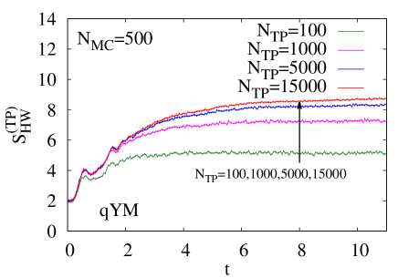
Figure 1 shows the time evolution of the HW entropy calculated in the TP method with the following test-particle numbers, $N_{\rm TP}=100,1000,5000$ and $15000$. The MC sample number is taken to be $N_{\rm MC}=500$. The statistical errors are estimated for ${N_{\mathrm{MC}}}$ samples from a standard deviation. We note that the calculated HW entropy at each $t$ tends to increase along with increasing $N_{\rm TP}$, which is an artifact due to the small number of the test particles $N_{\rm TP}$ and discussed later. Apart from tiny fluctuations, all the calculation show that the HW entropy first increases in time with a small oscillatory behavior being accompanied; its local maxima are seen around $t\simeq 0.5$ and $1.7$. We note that a similar behavior is also seen in Ref. TsaiMuller .

Entropy evaluated by the TP method has a (unphysical) maximum depending on $N_{\rm TP}$, which causes apparent saturation at large $t$ in Fig. 1. In fact, when the system is chaotic and the phase space volume is very large, all the test particles will be so separated from each other in the phase space at later time that only the $i=j$ terms in Eq. (18) will remain. In this limiting case, the HW entropy as given in (18) is evaluated as follows;

$$S_{\mathrm{HW}}^{\mathrm{(TP)}}\to -\left\langle\left[\log\left(\frac{2^{D}}{{N_{\mathrm{TP}}}}\right)-\Delta Q^{2}/\hbar-P^{2}/\Delta\hbar\right]\right\rangle_{QP}$$

$$=D-D\log{2}+\log{{N_{\mathrm{TP}}}}\ ,$$ (23)

which gives the inevitable upper limit of $S_{\rm HW}^{({\rm TP})}$. In Appendix A, we examine the HW entropy of an inverted harmonic oscillator, for which $S_{\rm HW}$ can be calculated analytically and is found to increase permanently. At later times, ${S_{\mathrm{HW}}}$ is underestimated with small ${N_{\mathrm{TP}}}$ values because of the upper limit discussed above. By comparison, ${S_{\mathrm{HW}}}$ at early times is calculated precisely in the TP method, as long as ${N_{\mathrm{TP}}}$ is large enough for ${S_{\mathrm{HW}}}$ to converge.

From the above argument, ${S_{\mathrm{HW}}}(t)$ would be obtained reliably as an extrapolated value in the limit of ${N_{\mathrm{TP}}}\to\infty$. The extrapolation should be made in the ${N_{\mathrm{TP}}}$ range, where the limiting value is larger than the HW entropy to be obtained. The limiting values are $S_{\mathrm{HW}}^{\mathrm{(TP)}}=5.2,7.5,9.1$ and $10.2$ for ${N_{\mathrm{TP}}}=100,1000,5000$ and $15000$, respectively. The large-t values found in Fig. 1 are close to these limiting values for smaller ${N_{\mathrm{TP}}}$, i.e., ${N_{\mathrm{TP}}}=100$ and $1000$. Thus we see that the saturation behavior seen for smaller values of $N_{\mathrm{TP}}$ may be an artifact of the TP method. In contrast , the large-t values for $N_{\mathrm{TP}}=5000$ and $15000$ in Fig. 1 are well below the limiting values ($9.1$ and $10.2$), found free from the above mentioned artifact, and can be used to obtain the extrapolated value at ${N_{\mathrm{TP}}}\to\infty$, as discussed later in Subsec. 4.4. Thus we conclude that the entropy production of the “quantum Yang-Mills” system can be well described with the use of HW entropy as calculated with the TP method with sufficiently large number of the test particles.

4.3 Numerical results with tsMC method

Next, we show the numerical results of the HW entropy in qYM in the tsMC method using the formula Eq. (19).

Figure 2: Time dependence of HW entropy calculated by using tsMC method.

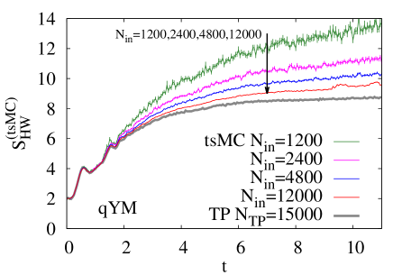
Figure 2 shows the time evolution of the HW entropy calculated in the tsMC method with the sample numbers $N_{\rm in}=1200,2400,4800$ and $12000$. $N_{\rm out}$ is taken to be the same as $N_{\rm in}$. The errors attached to $S_{\rm HW}$ in the present figure is estimated only for the Monte-Carlo integrals outside of $\log$ in Eq. (19), and those from the integral inside the $\log$ is not taken into account, which causes an additional systematic error.

We see that the larger the value of $N_{\rm in}$, the smaller the HW entropy, which is an opposite dependence on the sample number to that in the TP method. Nevertheless the gross behavior in the time evolution of the HW entropy is quite similar in the two methods apart from the tiny fluctuations; After showing an oscillatory behavior in a first short period, it increases in a monotonous way and its growth rate decreases gradually. More quantitative comparison of the two methods will be presented in the next subsection.

4.4 Comparison of the two methods

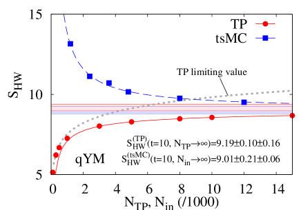
Figure 3 shows the HW entropy at $t=10$ as a function of $N_{\rm TP}$ ($N_{\rm in}$) in the TP (tsMC) method. We fit a linear function $f(t)=at+b$ to the calculated $S_{\mathrm{HW}}(t)$ data in the range $10-\Delta t\leq t\leq 10+\Delta t\ (\Delta t=1)$, and adopt $f(t=10)$ as the HW entropy value at $t=10$. This procedure provides a smoother curve and reduces the errors coming from fluctuations compared to directly using the raw data.

The HW entropy in the TP method becomes larger with increasing $N_{\rm TP}$ as already mentioned; At $t=10$, $S_{\rm HW}\simeq 5.1$ for $N_{\rm TP}=100$ and $S_{\rm HW}\simeq 8.7$ for $N_{\rm TP}=15000$. We also show the fit results to the data for larger samples, say $N_{TP}\geq 5000$, with a fit function,

$$f(N)=a-\frac{b}{N^{c}}.$$ (24)

The extrapolated value to $N_{\rm TP}\rightarrow\infty$ is $9.19\pm 0.10$. When we use other fit functions such as $f(N)=a-b/(N/c+1)$ and $f(N)=a-b/N+c/N^{2}$, the fit results have differences with a standard deviation of $0.16$, which should be considered as a systematic error. Thus the HW entropy in the TP method is obtained as

$$S_{\mathrm{HW}}^{\mathrm{(TP)}}(t=10)=9.19\pm 0.10~{}\mathrm{(stat.)}\pm 0.16~{}\mathrm{(syst.)}\ .$$ (25)

With increasing $N_{\rm in}$, the HW entropy calculated in the tsMC method decreases, which is an opposite behavior to that in the TP method as noted before. At $t=10$, $S_{\rm HW}\simeq 13.2$ for $N_{\rm in}=1200$ and $S_{\rm HW}\simeq 9.5$ for $N_{\rm in}=12000$. We also show the fit results to the data. We adopt Eq. (24) for the fit function. From the fit results, the HW entropy in the tsMC method is found to be

$$S_{\mathrm{HW}}^{\mathrm{(tsMC)}}(t=10)=9.01\pm 0.21~{}\mathrm{(stat.)}\pm 0.06~{}\mathrm{(syst.)}\ ,$$ (26)

where the central value and the statistical error are obtained from the fit using Eq. (24), and the systematic error is evaluated from the fits using several fit functions as done in the TP method.

Figure 3: HW entropy in qYM at $t=10$ as a function of ${N_{\mathrm{TP}}}$ (${N_{\mathrm{MC}}}$), and its extrapolation to infinitely large ${N_{\mathrm{TP}}}$ (${N_{\mathrm{MC}}}$) in the TP (tsMC) method. Filled circles (squares) show TP (tsMC) results, and the solid (dashed) line shows a fit function to TP (tsMC) results. The dotted line is limiting value given by Eq. (23). The shaded areas show the extrapolated value in the limit of ${N_{\mathrm{TP}}},{N_{\mathrm{MC}}}\to\infty$.

4.5 Discussions

The time evolution of the HW entropies obtained in the TP and tsMC methods shows a similar behavior with each other: The HW entropy increases with an oscillatory behavior in the early stage, then shows a monotonous increase with a decreasing rate. The HW entropy at each $t$ in the TP method increases along with ${N_{\mathrm{TP}}}$, while it decreases with increasing ${N_{\mathrm{in}}}$ in the tsMC method. Thus we can guess that the real value of the HW entropy lies between the results in the TP and tsMC methods. Actually, the extrapolated values at $t=10$, $S_{\mathrm{HW}}^{\mathrm{(TP)}}(t=10)=9.19\pm 0.10\pm 0.16$ at ${N_{\mathrm{TP}}}\to\infty$ and $S_{\mathrm{HW}}^{\mathrm{(tsMC)}}(t=10)=9.01\pm 0.21\pm 0.06$ at ${N_{\mathrm{in}}}\to\infty$ in the TP and tsMC methods respectively, are consistent with each other within the error. These results are also in agreement with that in Ref.TsaiMuller .

These two methods, TP and tsMC methods, give consistent results after $N\rightarrow\infty$ extrapolation. On the other hand, with finite number of ${N_{\mathrm{TP}}}$ and $N_{\rm in}$, they could give seemingly inconsistent results depending on the dynamics. We here have a deeper look at this issue. In the tsMC method, the entropy seems to keep increasing even for the later time, in contrast to the results in the TP method with finite ${N_{\mathrm{TP}}}$ and in Ref.TsaiMuller . The discrepancy may come from the special shape of the potential: there are two flat directions in the potential for the qYM system, although the width of them tends to shrink at large distances. Then, the classical trajectory can keep growing along the flat direction, which would cause an unlimited spreading of the Husimi function and a permanent increase of the HW entropy calculated in the semiclassical approximation. (In the case of the TP methods, there exists limiting value of the HW entropy depending on ${N_{\mathrm{TP}}}$, which gives rise to the apparent saturation of $S$ at large $t$. ) By comparison, it is shown that the exact energy spectra of the qYM are all discrete ones, because of the shrinking width leading to an increase of the kinetic energy due to the uncertainty relation, although the volume of $\{(p,q)|H(p,q)\leq E\}$ is infinite Simon1983 . Note that the discrete spectra implies that the wave functions of the energy eigen states are all bound. Thus the corresponding Husimi function would not have a support at the infinite distance due to the quantum effect, and the HW entropy may not show the ever increasing behavior but have a saturated value. This plausible conjecture can only be confirmed by a full quantum calculation beyond the semiclassical approximation. Such a calculation is beyond the scope of the present work and will be left as a future work. Instead, we shall take another model, which is a modified version of the qYM one free from flat directions in its potential.

5 Modified quantum Yang-Mills model

Figure 4: Time dependence of HW entropy by using TP method in modified qYM.

Figure 5: Time dependence of HW entropy by using tsMC method in modified qYM.

Figure 6: HW entropy in mqYM at $t=10$ as a function of ${N_{\mathrm{TP}}}$ (${N_{\mathrm{MC}}}$), and its extrapolation to infinitely large ${N_{\mathrm{TP}}}$ (${N_{\mathrm{MC}}}$) in the TP (tsMC) method. Filled circles (squares) show TP (tsMC) results, and the solid (dashed) line shows a fit function to TP (tsMC) results. The dotted line is limiting value given by Eq. (23). The shaded areas show the extrapolated value in the limit of ${N_{\mathrm{TP}}},{N_{\mathrm{MC}}}\to\infty$.

Let us consider the model in which quartic potential terms are added to the qYM Hamiltonian;

$$H=\frac{p_{1}^{2}}{2m}+\frac{p_{1}^{2}}{2m}+\frac{1}{2}g^{2}q_{1}^{2}q_{2}^{2}+\frac{\epsilon}{4}q_{1}^{4}+\frac{\epsilon}{4}q_{2}^{4}.$$ (27)

We call the system “modified quantum Yang-Mills (mqYM)”. The system is studied in Ref.Sugita-Aiba2002 ; Sugita03 with $g^{2}<0$ in the context of chaos. It is apparent that there is no flat direction in the potential due to the quartic terms. We take $g^{2}=1$ and $\epsilon=0.1$ in the Hamiltonian, Eq. (27). The mqYM system is found to be integrable with $\epsilon/g^{2}=1,1/3$ and $\infty$ Baker:1995bp ; Sugita-Aiba2002 . Our choice of $\epsilon/g^{2}=0.1$ is well apart from the integrable region. Since $\epsilon$ is not very large, the HW entropy shows a similar behavior to that in qYM at early times, as shown later.

In this section, we shall calculate the HW entropy of the mqYM system in the TP and tsMC methods . The analyses are carried out in a similar way to those for the qYM system.

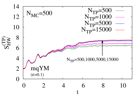
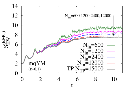
In Figs. 4 and 5, we show the time evolution of the HW entropy in mqYM calculated using the TP (${N_{\mathrm{TP}}}=500,1000,5000$ and $15000$ with ${N_{\mathrm{MC}}}=500$) and tsMC (${N_{\mathrm{in}}}=600,1200,2400$ and $12000$) methods, respectively. $N_{\rm out}$ is taken to be the same as ${N_{\mathrm{in}}}$ for tsMC.

The distribution function in Eq. (22) is used as the initial condition, and the statistical errors are estimated for ${N_{\mathrm{MC}}}$ (${N_{\mathrm{in}}}$) samples from a standard deviation in the TP (tsMC) method, as in the qYM cases.

Both of the calculated results show that the HW entropy first increases with an oscillatory behavior and tends to saturate at later times, $t\gtrsim 6$. The later-time ${S_{\mathrm{HW}}}$ values depend on the sample number, ${N_{\mathrm{TP}}}$ and ${N_{\mathrm{in}}}$; With increasing ${N_{\mathrm{TP}}}$ (${N_{\mathrm{in}}}$), the HW entropy increases (decreases) in the TP (tsMC) method. These are the features also found in qYM. By comparison, it should be noted that there seems to be saturation of ${S_{\mathrm{HW}}}$ both in the TP and tsMC methods in mqYM, in contrast to qYM. This may be originated from the finite phase space volume where the Husimi function has a support.

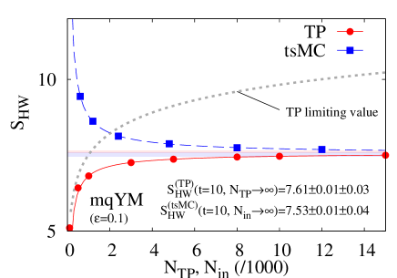
In Fig. 6, we show the HW entropy at $t=10$ as a function of ${N_{\mathrm{TP}}}$ or ${N_{\mathrm{in}}}$. We fit a linear function to calculated $S_{\mathrm{HW}}(t)$ results in the range $9<t<11$, and adopt $f(t=10)$ as the HW entropy value at $t=10$. In the TP method, $S_{\mathrm{HW}}^{\mathrm{(TP)}}(t=10)\simeq 6.4$ and $7.5$ for ${N_{\mathrm{TP}}}=500$ and $15000$, respectively. In tsMC, we find $S_{\rm HW}^{\mathrm{(tsMC)}}(t=10)\simeq 9.4$ and $7.7$ for ${N_{\mathrm{in}}}=600$ and $12000$, respectively.

The extrapolated values of ${S_{\mathrm{HW}}}$ at ${N_{\mathrm{TP}}}\to\infty$ and ${N_{\mathrm{in}}}\to\infty$ are found to be

$$S_{\mathrm{HW}}^{\mathrm{(TP)}}(t=10)=7.61\pm 0.01\mathrm{(stat.)}\pm 0.03\mathrm{(syst.)}\ ,$$ (28)

$$S_{\mathrm{HW}}^{\mathrm{(tsMC)}}(t=10)=7.53\pm 0.01\mathrm{(stat.)}\pm 0.04\mathrm{(syst.)}\ ,$$ (29)

in the TP and tsMC methods, respectively. The central values and the statistical errors are obtained from the fit using Eq. (24), and the systematic error is evaluated from the fits using several fit functions. These two values are consistent with each other within the error.

The observation shows that the two methods, tsMC and TP, are especially effective for such a potential which bounds Husimi function in finite region. Thus, we are confident of the validity of the two methods in the mqYM system.

6 Summary

We have discussed entropy creation in isolated quantum systems by using the Husimi-Wehrl entropy evaluated in a semiclassical treatment. The semiclassical treatment is known to be useful in some of the systems such as the inflation in early universe and the early stage of relativistic heavy ion collisions. These systems are expected to bear instabilities and/or chaoticities in their classical counter systems, then the smearing of the phase space distribution by the minimal wave packet causes the entropy production in terms of the Wehrl entropy or the $H$ function of Boltzmann even in isolated quantum systems. This is nothing but the Husimi-Wehrl entropy, the Wehrl entropy obtained by using the Gaussian smeared Wigner function (Husimi function) for the phase space distribution.

The semiclassical time evolution of the Husimi function is given by solving a classical equation of motion and smearing with a Gaussian packet. Combining this semiclassical treatment with the Monte-Carlo numerical integral technique, we have developed two methods, the test-particle (TP) method and the two-step Monte Carlo (tsMC) method. We have applied these two methods to quantum mechanical systems in two dimensions, the quantum Yang-Mills (qYM) and the modified quantum Yang-Mills (mqYM) systems. The classical counter systems of these are known to be chaotic. We have demonstrated that the Husimi-Wehrl entropy obtained in the TP (tsMC) method approaches the converged value from below (from above) with an increasing sample number, then we can guess the true value of HW entropy. We have further found that the results of the TP and tsMC methods in the infinite sampling number limit are consistent within the error. Therefore, the simultaneous application of the two methods ensures the reliability of the results of the Husimi-Wehrl entropy at a given time.

The extension of our methods to a multidimensional system is straightforward. We expect that these methods are useful in systems with many degrees of freedom such as the quantum field theory. These methods are, in principle, applicable to higher-dimensional problems, and we have confirmed that they actually work in three and four dimensional systems. In higher dimensions, we need much more Monte-Carlo samples to obtain statistically reliable results, and it would be necessary to make some approximations for practical purposes. Work in this direction is in progress.

Appendix A HW entropy in inverted harmonics

The inverted harmonic oscillator (IHO) is an unstable system, where the Hamiltonian is given as

$$H=\frac{p^{2}}{2m}-\frac{1}{2}\lambda^{2}q^{2}.$$ (30)

In this system, the classical trajectories are not restricted in a finite region, but extends to infinitely large spatial and momentum regions. While this unbounded nature makes the numerical calculation difficult, the analytic expression of the HW entropy is known KMOS . Then by comparing the numerical results with the analytic solution, we can examine the validity and the precision of the numerical methods.

A.1 Analytic solution

When the initial distribution of Wigner function is given by a Gaussian,

$$f_{W}(p,q;t=0)=2\exp\left(-\frac{1}{\hbar\omega}p^{2}-\frac{\omega}{\hbar}q^{2}\right),$$ (31)

the time evolution of the HW entropy is obtained analytically KMOS . Since the potential is quadratic, the semiclassical analysis is exact, and the time evolution of the Wigner function is calculated by solving the classical equation of motion. The HW entropy at time $t$ is given as KMOS ,

$$S_{HW}(t)=\log\frac{\sqrt{A(t)}}{2}+1\ ,$$ (32)

$$A(t)=2(\sigma\rho\cosh(2\lambda t)+1+\delta\delta^{\prime})\ ,$$ (33)

$$\sigma=\frac{\lambda^{2}+\omega^{2}}{2\lambda\omega}\ ,\quad\delta=\frac{\lambda^{2}-\omega^{2}}{2\lambda\omega}\ ,$$ (34)

$$\rho=\frac{\Delta^{2}+\lambda^{2}}{2\Delta\lambda}\ ,\quad\delta^{\prime}=\frac{\Delta^{2}-\lambda^{2}}{2\Delta\lambda}.$$ (35)

Figure 7: Time dependence of the HW entropy of the inverted harmonic oscillator in the TP method.

A.2 Numerical results with TP

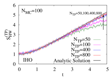
Figure 7 shows the time evolution of the HW entropy of IHO calculated in the TP method with ${N_{\mathrm{TP}}}=50-800$. We find that the TP method can well describe the time evolution of the HW entropy at early times, and that numerical results show saturated behavior in later times. Since there exists a limiting value of ${S_{\mathrm{HW}}}$ in the TP method as discussed in Subsec. 4.2, we need to take a large number of ${N_{\mathrm{TP}}}$ to describe a large amount of entropy production. It should be noted that numerical results converge in the limit of ${N_{\mathrm{TP}}}\to\infty$, and the converged result well describe the analytic result.

Figure 8: Time dependence of the HW entropy of the inverted harmonic oscillator in the tsMC method.

A.3 Numerical results with tsMC

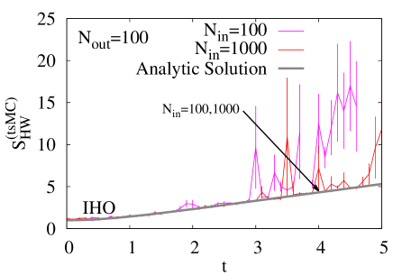
Figure 8 shows the time evolution of the HW entropy of IHO in the tsMC method with ${N_{\mathrm{in}}}=N_{\mathrm{out}}=100$ and $1000$. We find that numerical results are consistent with the analytic solution at early times $t\leq 3$, but that the numerical results tend to overestimate the analytic results and numerical errors become very large at later times. The large error would come from the poor overlap between the Wigner function and the coarse-graining Gaussian function at later time, which makes importance sampling spoiled. On the other hand, the systematic overestimation may be due to the lack of sampling points in the Monte-Carlo integration in the logarithmic function (See Eq. (19)). We note here that the statistical-error estimation is performed only for the Monte-Carlo integration outside the log.

References

- (1) J. von Neumann, Gött. Nach. 1927, 273 (1927); ”Mathematische Grundlagen der Quantenmechanik” (Springer, Berlin, 1932).
- (2) E.P. Wigner, Phys. Rev. 40, 749 (1932).
- (3) H. Groenewold, Physica 12, 405 (1946).
- (4) J.E. Moyal, Proc. Cambridge Phil. Soc. 45, 99 (1949).
- (5) M. Hillery, R. F. O’Connell, M. O. Scully and E. P. Wigner, Phys. Rept. 106, 121 (1984).
- (6) Hai-Woong Lee, Phys. Rep. 259 (1995), 147.
- (7) T. L. Curtright, D. B. Fairlie and C. K. Zachos, “A concise treaties on quantum mechanics in phase space” (World Scientific, 2014).
- (8) K. Husimi, Proc. Phys. Math. Soc. Jpn. 22, 123 (1940).
- (9) K. Takahashi and N. Saito, Phys. Rev. Lett. 56, 645 (1985).
- (10) K. Takahashi, Prog. Theor. Phys. Suppl. 98, 109 (1989).
- (11) A. Sugita, J. Phys. A 34, 9081 (2003).
- (12) A. Sugita and H. Aiba, Phys. Rev. E. 65, 036205 (2002).
- (13) A. Wehrl, Rev. Mod. Phys. 50, 221 (1978).
- (14) A. Anderson, J. J. Halliwell, Phys. Rev. D 48, 2753 (1993).
- (15) T. Kunihiro, B. Muller, A. Ohnishi and A. Schafer, Prog. Theor. Phys. 121, 555 (2009).
- (16) F. Mintert and K. Zyczkowski, Phys. Rev. A 69, 022317 (2004).
- (17) M. Abdel-Aty, Progress in Quantum Electronics 31, 1 (2007).
- (18) A. Wehrl, Rep. Math. Phys. 16, 353 (1979).
- (19) E. H. Lieb, Commun. Math. Phys. 62, 35 (1978).
- (20) A. Orlowski, H. Paul and G. Kastelewicz, Phys. Rev. A 52, 1621 (1995).
- (21) H. M. Tsai and B. Muller, Phys. Rev. E 85, 011110 (2012).
- (22) K. Takahashi, J. Phys. Soc. Jpn. 55, 762 (1986).
- (23) W. H. Zurek and J. P. Paz, Phys. Rev. Lett. 72, 2508 (1994).
- (24) C. Y. Wong, Phys. Rev. C 25, 1460 (1982).
- (25) G. F. Bertsch and S. Das Gupta, Phys. Rept. 160, 189 (1988).
- (26) N. Rostoker and M. N. Rosenbluth, Phys. Fluids 3, 1 (1960).
- (27) R. W. Hockney and J. W. Eastwood, ”Computer simulation using particles” (1988, CRC Press, London).
- (28) S. G. Matinyan, G. K. Savvidy, and N. G. Ter-Arutyunyan- Savvidy, Zh. Eksp. Teor. Fiz. 80, 830 (1981) [Sov. Phys. JETP 53, 421 (1981)].
- (29) B. Simon Ann. Phys 146 209-220 (1983).
- (30) S. Baker, V. Z. Enolsky and A. P. Fordy, Phys. Lett. A 201, 167 (1995).