A survey of recent results in (generalized) graph entropies

Abstract

The entropy of a graph was first introduced by Rashevsky [1] and Trucco [2] to interpret as the structural information content of the graph and serve as a complexity measure. In this paper, we first state a number of definitions of graph entropy measures and generalized graph entropies. Then we survey the known results about them from the following three respects: inequalities and extremal properties on graph entropies, relationships between graph structures, graph energies, topological indices and generalized graph entropies, complexity for calculation of graph entropies. Various applications of graph entropies together with some open problems and conjectures are also presented for further research.
Keywords: graph entropy, generalized graph entropy, shannon’s entropy, complex networks, information measures, graph energies, graph indices, structural information content, hierarchical graphs, chemical graph theory
AMS subject classification 2010: 94A17, 05C90, 92C42, 92E10

1 Introduction

Graph entropy measures play an important role in a variety of subjects, including information theory, biology, chemistry, and sociology. It was first introduced by Rashevsky [1] and Trucco [2]. Mowshowitz [3, 4, 5, 6] first defined and investigated the entropy of graphs, and Körner [7] introduced a different definition of graph entropy closely linked to problems in information and coding theory. In fact, there may be no “right” one or “good” one, since what may be useful in one domain may not be serviceable in another.

Distinct graph entropies have been used extensively to characterize the structures of graph-based systems in various fields. In these applications the entropy of a graph is interpreted as the structural information content of the graph and serves as a complexity measure. It is worth mentioning that two different approaches to measure the complexity of graphs have been developed: deterministic and probabilistic. The deterministic category encompasses the encoding, substructure count and generative approaches, while the probabilistic category includes measures that apply an entropy function to a probability distribution associated with a graph. The second category is subdivided into intrinsic and extrinsic subcategories. Intrinsic measures use structural features of a graph to partition the graph (usually the set of vertices or edges) and thereby determine a probability distribution over the components of the partition. Extrinsic measures impose an arbitrary probability distribution on graph elements. Both of these categories employ the probability distribution to compute an entropy value. Shannon’s entropy function is most commonly used, but several different families of entropy functions are also considered.

Actually, three survey papers [9, 10, 8] on graph entropy measures were published already. However, [9, 10] focused narrowly on the properties of Körner’s entropy measures and [8] provided an overview of the most well-known graph entropy measures which contains not so many results and only concepts were preferred. Here we focus on the development of graph entropy measures and aim to provide a broad overview of the main results and applications of the most well-known graph entropy measures.

Now we start our survey by providing some mathematical preliminaries. Note that all graphs discussed in this chapter are assumed to be connected.

Definition 1.1

We use $G=(V,E)$ with $|V|<\infty$ and $E\subseteq{V\choose 2}$ to denote a finite undirected graph. If $G=(V,E)$, $|V|<\infty$ and $E\subseteq V\times V$, then $G$ is called a finite directed graph. We use $\mathcal{G}_{\cup C}$ to denote the set of finite undirected connected graphs.

Definition 1.2

Let $G=(V,E)$ be a graph. The quantity $d(v_{i})$ is called the degree of a vertex $v_{i}\in V$ where $d(v_{i})$ equals the number of edges $e\in E$ incident with $v_{i}$. In the following, we simply denote $d(v_{i})$ by $d_{i}$. If a graph $G$ has $a_{i}$ vertices of degree $\mu_{i}\ (i=1,2,\cdots,t)$, where $\Delta(G)=\mu_{1}>\mu_{2}>\cdots>\mu_{t}=\delta(G)$ and $\sum_{i=1}^{t}a_{i}=n$, we define the degree sequence of $G$ as $D(G)=[\mu_{1}^{a_{1}},\mu_{2}^{a_{2}},\cdots,\mu_{t}^{a_{t}}]$. If $a_{i}=1$, we use $\mu_{i}$ instead of $\mu_{i}^{1}$ for convenience.

Definition 1.3

The distance between two vertices $u,v\in V$, denoted by $d(u,v)$, is the length of a shortest path between $u,v\in V$. A path $P$ connecting $u$ and $v$ in $G$ is called a geodesic path if the length of the path $P$ is exactly $d(u,v)$. We call $\sigma(v)=max_{u\in V}d(u,v)$ the eccentricity of $v\in V$. In addition, $r(G)=min_{v\in V}\sigma(v)$ and $\rho(G)=max_{v\in V}\sigma(v)$ are called the radius and diameter of $G$, respectively. Without causing any confusion, we simply denote $r(G),\rho(G)$ as $r,\rho$, respectively.

A path graph is a simple graph whose vertices can be arranged in a linear sequence in such a way that two vertices are adjacent if they are consecutive in the sequence, and are nonadjacent otherwise. Likewise, a cycle graph on three or more vertices is a simple graph whose vertices can be arranged in a cyclic sequence in such a way that two vertices are adjacent if they are consecutive in the sequence, and are nonadjacent otherwise. Denote by $P_{n}$ and $C_{n}$ the path graph and the cycle graph on $n$ vertices, respectively.

A connected graph without any cycle is a tree. A star of order $n$, denoted by $S_{n}$, is the tree with $n-1$ pendant vertices. Its unique vertex with degree $n-1$ is called the center vertex of $S_{n}$. A simple connected graph is called unicyclic if it has exactly one cycle. We use $S^{+}_{n}$ to denote the unicyclic graph obtained from the star $S_{n}$ by adding to it an edge between two pendant vertices of $S_{n}$. Observe that a tree and a unicyclic graph of order $n$ have exactly $n-1$ and $n$ edges, respectively. A bicyclic graph is a graph of order $n$ with $n+1$ edges. A tree is called a double star $S_{p,q}$ if it is obtained from $S_{p+1}$ and $S_{q}$ by identifying a leaf of $S_{p+1}$ with the center vertex of $S_{q}$. So, for the double star $S_{p,q}$ with $n$ vertices, we have $p+q=n$. We call a double star $S_{p,q}$ balanced if $p=\lfloor\frac{n}{2}\rfloor$ and $q=\lceil\frac{n}{2}\rceil$. A comet is a tree composed of a star and a pendant path. For any integers $n$ and $t$ with $2\leq t\leq n-1$, we denote by $CS(n,t)$ the comet of order $n$ with $t$ pendant vertices, i.e., a tree formed by a path $P_{n-t}$ of which one end vertex coincides with a pendant vertex of a star $S_{t+1}$ of order $t+1$.

Definition 1.4

The $j$-sphere of a vertex $v_{i}$ in $G=(V,E)\in\mathcal{G}_{\cup C}$ is defined by the set

$$S_{j}(v_{i},G):=\{v\in V|d(v_{i},v)=j,j\geq 1\}.$$

Definition 1.5

Let $X$ be a discrete random variable by using alphabet $\mathcal{A}$, and $p(x_{i})=Pr(X=x_{i})$ the probability mass function of $X$. The mean entropy of $X$ is then defined by

$$H(X):=\sum_{x_{i}\in\mathcal{A}}p(x_{i})\log(p(x_{i})).$$

The concept of graph entropy introduced by Rashevsky in [1] and Trucco in [2] is used to measure structural complexity. Several graph invariants such as the number of vertices, the vertex degree sequence, and extended degree sequences have been used in the construction of graph entropy measures. The main graph entropy measures can be divided into two classes: classical measures and parametric measures. Classical measures, denoted by $I(G,\tau)$, are defined relative to a partition of a set $X$ of graph elements induced by an equivalence relation $\tau$ on $X$. More precisely, let $X$ be a set of graph elements (typically vertices), and let $\{X_{i}\}$, $1\leq i\leq k$, be a partition of $X$ induced by $\tau$. Suppose further that $p_{i}:=\frac{|X_{i}|}{|X|}$. Then

$$I(G,\tau)=-\sum\limits_{i=1}^{k}p_{i}\log(p_{i}).$$

As mentioned in [8], Rashevsky [1] defined the following graph entropy measure

$$I^{V}(G):=-\sum\limits_{i=1}^{k}\frac{|N_{i}|}{|V|}\log\left(\frac{|N_{i}|}{|V|}\right)$$ (1.1)

where $|N_{i}|$ denotes the number of topologically equivalent vertices in the $i$-th vertex orbit of $G$ and $k$ is the number of different orbits. Vertices are considered as topologically equivalent if they belong to the same orbit of a graph. According to [11], we have that if a graph $G$ is vertex-transitive [12, 13], then $I^{V}(G)=0$. Additionally, Trucco [2] introduced a similar graph entropy measure

$$I^{E}(G):=-\sum\limits_{i=1}^{k}\frac{|N_{i}^{E}|}{|E|}\log\left(\frac{|N_{i}^{E}|}{|E|}\right)$$ (1.2)

where $|N^{E}_{i}|$ stands for the number of edges in the $i$-th edge orbit of $G$. These two entropies are both classical measures, in which special graph invariants (e.g., numbers of vertices, edges, degrees, distances, etc.) and equivalence relations have given rise to these measures of information contents. And thus far, a number of specialized measures have been developed that are used primarily to characterize the structural complexity of chemical graphs [14, 15, 16].

In recent years, instead of inducing partitions and determining their probabilities, researchers assign a probability value to each individual element of a graph to derive graph entropy measures. This leads to the other class of graph entropy measures: parametric measures. Parametric measures are defined on graphs relative to information functions. Such functions are not identically zero and map graph elements (typically vertices) to nonnegative reals. Now we give the precise definition for entropies belonging to parametric measures.

Definition 1.6

Let $G\in\mathcal{G}_{\cup C}$ and let $S$ be a given set, e.g., a set of vertices or paths, etc. Functions $f:S\rightarrow\mathbb{R}_{+}$ play a role in defining information measures on graphs and we call them information functions of $G$.

Definition 1.7

Let $f$ be an information function of $G$. Then

$$p^{f}(v_{i}):=\frac{f(v_{i})}{\sum\limits_{j=1}^{|V|}f(v_{j})}.$$

Obviously,

$$p^{f}(v_{1})+p^{f}(v_{2})+\cdots+p^{f}(v_{n})=1,\ \text{where}\ n=|V|.$$

Hence, $(p^{f}(v_{1}),p^{f}(v_{2}),\cdots,p^{f}(v_{n}))$ forms a probability distribution.

Definition 1.8

Let $G$ be a finite graph and let $f$ be an information function of $G$. Then

$$I_{f}(G):=-\sum\limits_{i=1}^{|V|}\frac{f(v_{i})}{\sum_{j=1}^{|V|}f(v_{j})}\log\frac{f(v_{i})}{\sum_{j=1}^{|V|}f(v_{j})}$$ (1.3)

$$I_{f}^{\lambda}(G):=\lambda\left(\log(|V|)+\sum\limits_{i=1}^{|V|}\frac{f(v_{i})}{\sum_{j=1}^{|V|}f(v_{j})}\log\frac{f(v_{i})}{\sum_{j=1}^{|V|}f(v_{j})}\right)$$ (1.4)

are families of information measures representing structural information content of $G$, where $\lambda>0$ is a scaling constant. $I_{f}$ is the entropy of $G$ which belongs to parametric measures and $I_{f}^{\lambda}$ its information distance between maximum entropy and $I_{f}$.

The meaning of $I_{f}(G)$ and $I_{f}^{\lambda}(G)$ has been investigated by calculating the information content of real and synthetic chemical structures [17]. Also, the information measures were calculated using specific graph classes to study extremal values and, hence, to detect the kind of structural information captured by the measures.

In fact, there also exist graph entropy measures based on integral though we do not focus on them in this paper. We introduce simply here one such entropy: the tree entropy. For more details we refer to [18, 19]. A graph $G=(V,E)$ with a distinguished vertex $o$ is called a rooted graph, which is denoted by $(G,o)$ here. A rooted isomorphism of rooted graphs is an isomorphism of the underlying graphs that takes the root of one to the root of the other. The simple random walk on $G$ is the Markov chain whose state space is $V$ and whose transition probability from $x$ to $y$ equals the number of edges joining $x$ to $y$ divided by $d(x)$. The average degree of $G$ is $\frac{\sum_{x\in V}d(x)}{|V|}$.

Let $p_{k}(x;G)$ denote the probability that the simple random walk on $G$ started at $x$ and back at $x$ after $k$ steps. Given a positive integer $R$, a finite rooted graph $H$, and a probability distribution $\rho$ on rooted graphs, let $p(R,H,\rho)$ denote the probability that $H$ is rooted isomorphic to the ball of radius $R$ about the root of a graph chosen with distribution $\rho$. Define the expected degree of a probability measure $\rho$ on rooted graphs to be

$$\overline{d}(\rho):=\int d(o)d\rho(G,o).$$

For a finite graph $G$, let $U(G)$ denote the distribution of rooted graphs obtained by choosing a uniform random vertex of $G$ as root of $G$. Suppose that $\langle G_{n}\rangle$ is a sequence of finite graphs and that $\rho$ is a probability measure on rooted infinite graphs. We say that the random weak limit of $\langle G_{n}\rangle$ is $\rho$ if for any positive integer $R$, any finite graph $H$, and any $\epsilon>0$, we have $\lim\limits_{n\rightarrow\infty}P[|p(R,H,U(G_{n}))-p(R,H,\rho)|>\epsilon]=0$.

Lyons [18] proposed the tree entropy of a probability measure $\rho$ on rooted infinite graphs

$$\textbf{h}(\rho):=\int\left(\log d(o)-\sum_{k\geq 1}\frac{1}{k}p_{k}(o,G)\right)d\rho(G,o).$$

For labeled networks, i.e., labeled graphs, Lyons [19] also gave a definition of information measure, which is more general than the tree entropy.

Definition 1.9

[19] Let $\rho$ be a probability measure on rooted networks. We call $\rho$ unimodular if

$$\int\sum_{x\in V(G)}f(G,o,x)d\rho(G,o)=\int\sum_{x\in V(G)}f(G,x,o)d\rho(G,o)$$

for all non-negative Borel functions $f$ on locally finite connected networks with an ordered pair of distinguished vertices that is invariant in the sense that for any (non-rooted) network isomorphism $\gamma$ of $G$ and any $x,y\in V(G)$, we have $f(\gamma G,\gamma x,\gamma y)=f(G,x,y)$.

Actually, following the seminal paper of Shannon [20], many generalizations of the entropy measure have been proposed. An important example of such a measure is called the Rényi entropy [21] which is defined by

$$I_{\alpha}^{r}(P):=\frac{1}{1-\alpha}\log\left(\sum\limits_{i=1}^{n}(P_{i})^{\alpha}\right),\ \alpha\neq 1$$

where $n=|V|$ and $P:=(p_{1},p_{2},\cdots,p_{n})$. For further discussion of the properties of Rényi entropy, see [22]. Rényi and other general entropy functions allow for specifying families of information measures that can be applied to graphs. Like some generalized information measures that have been investigated in information theory, Dehmer and Mowshowitz call these families generalized graph entropies. And in [23], they introduced six distinct such entropies which are stated as follows.

Definition 1.10

Let $G=(V,E)$ be a graph on $n$ vertices. Then

$$I^{1}_{\alpha}(G) := \frac{1}{1-\alpha}\log\left(\sum\limits_{i=1}^{k}\left(\frac{|X_{i}|}{|X|}\right)^{\alpha}\right)$$ (1.5)

$$I^{2}_{\alpha}(G)_{f} := \frac{1}{1-\alpha}\log\left(\sum\limits_{i=1}^{n}\left(\frac{f(v_{i})}{\sum_{j=1}^{n}f(v_{j})}\right)^{\alpha}\right)$$ (1.6)

$$I^{3}_{\alpha}(G) := \frac{\sum\limits_{i=1}^{k}\left(\frac{|X_{i}|}{|X|}\right)^{\alpha}-1}{2^{1-\alpha}-1}$$ (1.7)

$$I^{4}_{\alpha}(G)_{f} := \frac{\sum\limits_{i=1}^{n}\left(\frac{f(v_{i})}{\sum_{j=1}^{n}f(v_{j})}\right)^{\alpha}-1}{2^{1-\alpha}-1}$$ (1.8)

$$I^{5}(G) := \sum\limits_{i=1}^{k}\frac{|X_{i}|}{|X|}\left[1-\frac{|X_{i}|}{|X|}\right]$$ (1.9)

$$I^{6}(G)_{f} := \sum\limits_{i=1}^{n}\frac{f(v_{i})}{\sum_{j=1}^{n}f(v_{j})}\left[1-\frac{f(v_{i})}{\sum_{j=1}^{n}f(v_{j})}\right]$$ (1.10)

where $X$ is a set of graph elements (typically vertices), $\{X_{i}\}$ for $1\leq i\leq k$ is a partition of $X$ induced by the equivalence relation $\tau$, $f$ is an information function of $G$ and $\alpha\neq 1$.

Parametric complexity measures have been proved useful in the study of complexity associated with machine learning. And Dehmer et al. [24] showed that generalized graph entropies can be applied to problems in machine learning such as graph classification and clustering. Interestingly, these new generalized entropies have been proved useful in demonstrating that hypotheses can be learned by using appropriate data sets and parameter optimization techniques.

This chapter is organized as follows. Section 2 shows some inequalities and extremal properties of graph entropies and generalized graph entropies. Relationships between graph structures, graph energies, topological indices and generalized graph entropies are presented in Section 3, and the last section is a simple summary.

2 Inequalities and extremal properties on (generalized) graph entropies

Thanks to the fact that graph entropy measures have been applied to characterize the structures and complexities of graph-based systems in various areas, identity and inequality relationships between distinct graph entropies have been a hot and popular research topic. In the meantime, extremal properties of graph entropies have also been widely studied and lots of results were obtained.

2.1 Inequalities for classical graph entropies and parametric measures

Most of the graph entropy measures developed thus far have been applied in mathematical chemistry and biology [14, 25, 8]. These measures have been used to quantify the complexity of chemical and biological systems that can be represented as graphs. Given the profusion of such measures, it is useful to prove bounds for special graph classes or to study interrelations among them. Dehmer et al. [26] gave interrelation between the parametric entropy and a classical entropy measure that is based on certain equivalence classes associated with an arbitrary equivalence relation.

Theorem 2.1

[26] Let $G=(V,E)$ be an arbitrary graph, and let $X_{i},\ 1\leq i\leq k$, be the equivalence classes associated with an arbitrary equivalence relation on $X$. Suppose further that $f$ is an information function with $f(v_{i})>|X_{i}|$ for $1\leq i\leq k$ and $c:=\frac{1}{\sum_{j=1}^{|V|}f(v_{j})}$. Then

$$\frac{1}{|X|}I_{f}(G) < c\cdot I(G,\tau)-\sum\limits_{i=1}^{k}\frac{|X_{i}|}{|X|}c\cdot\log(c)-\frac{\log(|X|)}{|X|}\sum\limits_{i=1}^{k}p^{f}(v_{i})$$

$$-\frac{1}{|X|}\sum\limits_{i=k+1}^{|V|}p^{f}(v_{i})\log(p^{f}(v_{i}))+\frac{1}{|X|}\sum\limits_{i=1}^{k}p^{f}(v_{i})\log\left(1+\frac{|X|}{c\cdot f(v_{i})}\right)$$

$$+\sum\limits_{i=1}^{k}\log\left(\frac{p^{f}(v_{i})}{|X|}+1\right).$$

Assume that $f(v_{i})>|X_{i}|$, $1\leq i\leq k$, for some special graph classes and take the set $X$ to be the vertex set $V$ of $G$. Three corollaries of the above theorem on the upper bounds of $I_{f}(G)$ can be obtained.

Corollary 2.2

[26] Let $S_{n}$ be a star graph on $n$ vertices and suppose that $v_{1}$ is the vertex with degree $n-1$. The remaining $n-1$ non-hub vertices are labeled arbitrarily. $v_{\mu}$ stands for a non-hub vertex. Let $f$ be an information function satisfying the conditions of Theorem 2.1. Let $V_{1}:=\{v_{1}\}$ and $V_{2}:=\{v_{2},v_{3},\cdots,v_{n}\}$ denote the orbits of the automorphism group of $S_{n}$ forming a partition of $V$. Then

$$I_{f}(S_{n}) < p^{f}(v_{1})\log\left(1+\frac{1}{p^{f}(v_{1})}\right)+p^{f}(v_{\mu})\log\left(1+\frac{1}{p^{f}(v_{\mu})}\right)$$

$$+\log(1+p^{f}(v_{1}))+\log(1+p^{f}(v_{\mu}))-\sum\limits_{i=2,i\neq\mu}^{n}p^{f}(v_{i})\log(p^{f}(v_{i}))$$

$$-(n-1)\cdot c\cdot\log[(n-1)c]-c\log(c).$$

Corollary 2.3

[26] Let $G_{n}^{I}$ be an identity graph (a graph possessing a single graph automorphism) on $n\geq 6$ vertices. $G_{n}^{I}$ has only the identity automorphism and therefore each orbit is a singleton set, i,e., $|V_{i}|=1,\ 1\leq i\leq n$. Let $f$ be an information function satisfying the conditions of Theorem 2.1. Then

$$I_{f}(G_{n}^{I})<\sum\limits_{j=1}^{n}p^{f}(v_{j})\log\left(1+\frac{1}{p^{f}(v_{j})}\right)+\sum\limits_{j=1}^{n}\log(1+p^{f}(v_{j}))-n\cdot c\cdot\log(c).$$

Corollary 2.4

[26] Let $G_{n}^{P}$ be a path graph on $n$ vertices and let $f$ be an information function satisfying the conditions of Theorem 2.1. If $n$ is even, $G_{n}^{P}$ posses $\frac{n}{2}$ equivalence classes $V_{i}$ and each $V_{i}$ contains $2$ vertices. Then

$$I_{f}(G_{n}^{P}) < \sum\limits_{j=1}^{\frac{n}{2}}p^{f}(v_{j})\log\left(1+\frac{1}{p^{f}(v_{j})}\right)+\sum\limits_{j=1}^{\frac{n}{2}}\log(1+p^{f}(v_{j}))$$

$$-\sum\limits_{j=\frac{n}{2}+1}^{n}p^{f}(v_{j})\log(1+p^{f}(v_{j}))-n\cdot c\cdot\log(2c).$$

If $n$ is odd, then there exist $n-\lfloor\frac{n}{2}\rfloor$ equivalence classes, $n-\lfloor\frac{n}{2}\rfloor-1$ that have $2$ elements and only one class containing a single element. This implies that

$$I_{f}(G_{n}^{P}) < \sum\limits_{j=1}^{n-\lfloor\frac{n}{2}\rfloor}p^{f}(v_{j})\log\left(1+\frac{1}{p^{f}(v_{j})}\right)+\sum\limits_{j=1}^{n-\lfloor\frac{n}{2}\rfloor}\log(1+p^{f}(v_{j}))$$

$$-\sum\limits_{j=n-\lfloor\frac{n}{2}\rfloor+1}^{n}p^{f}(v_{j})\log(p^{f}(v_{j}))-(n-\lfloor\frac{n}{2}\rfloor-1)\cdot 2c\cdot\log(2c)$$

$$-c\cdot\log(c).$$

Assuming different initial conditions, Dehmer et al. [26] derived additional inequalities between classical and parametric measures.

Theorem 2.5

[26] Let $G$ be an arbitrary graph and $p^{f}(v_{i})<|X_{i}|$. Then

$$\frac{1}{|X|}I_{f}(G) > I(G,\tau)-\frac{1}{|X|}\sum\limits_{i=k+1}^{|V|}p^{f}(v_{i})\log(p^{f}(v_{i}))-\frac{\log(|X|)}{|X|}\sum\limits_{i=1}^{k}p^{f}(v_{i})$$

$$-\frac{1}{|X|}\sum\limits_{i=1}^{k}|X_{i}|\log\left(1+\frac{|X|}{|X_{i}|}\right)-\sum\limits_{i=1}^{k}\log\left(1+\frac{|X_{i}|}{|X|}\right).$$

Theorem 2.6

[26] Let $G$ be an arbitrary graph with $p_{i}$ being the probabilities such that $p_{i}<f(v_{i})$. Then

$$\frac{1}{c}I(G,\tau) > I_{f}(G)+\frac{\log(c)}{c}+\sum\limits_{i=k+1}^{|V|}p^{f}(v_{i})\log(p^{f}(v_{i}))$$

$$-\sum\limits_{i=1}^{k}\log(p^{f}(v_{i}))-\sum\limits_{i=1}^{k}\log\left(1+\frac{1}{p^{f}(v_{i})}\right)(1+p^{f}(v_{i})).$$

For identity graphs, they also obtained a general upper bound for the parametric entropy measure.

Corollary 2.7

[26] Let $G_{n}^{I}$ be an identity graph on $n$ vertices. Then

$$I_{f}(G_{n}^{I}) < \log(n)-c\cdot\log(c)+\sum\limits_{i=1}^{n}\log(p^{f}(v_{i}))$$

$$+\sum\limits_{i=1}^{n}\log\left(1+\frac{1}{p^{f}(v_{i})}\right)(1+p^{f}(v_{i})).$$

2.2 Graph entropy inequalities with information functions $f^{V}$, $f^{P}$ and $f^{C}$

In complex networks, information-theoretical methods are important for analyzing and understanding information processing. One major problem is to quantify structural information in networks based on so-called information functions. Considering a complex network as an undirected connected graph and based on such information functions, one can directly obtain different graphs entropies.

Now we define two information functions $f^{V}(v_{i}),\ f^{P}(v_{i})$, based on metrical properties of graphs, and a novel information function $f^{C}(v_{i})$, based on a vertex centrality measure.

Definition 2.1

[27] Let $G=(V,E)\in\mathcal{G}_{\cup C}$. For a vertex $v_{i}\in V$, we define the information function

$$f^{V}(v_{i}):=\alpha^{c_{1}|S_{1}(v_{i},G)|+c_{2}|S_{2}(v_{i},G)|+\cdots+c_{\rho}|S_{\rho}(v_{i},G)|},\quad c_{k}>0,\ 1\leq k\leq\rho,\ \alpha>0,$$

where the $c_{k}$ are arbitrary real positive coefficients, $S_{j}(v_{i},G)$ denotes the $j$-sphere of $v_{i}$ regarding $G$ and $|S_{j}(v_{i},G)|$ its cardinality, respectively.

Before giving the definition of the information function $f^{P}(v_{i})$, we introduce the following concepts first.

Definition 2.2

[27] Let $G=(V,E)\in\mathcal{G}_{UC}$. For a vertex $v_{i}\in V$ we determine the set $S_{j}(v_{i},G)=\{v_{u_{j}},v_{w_{j}},\cdots,v_{x_{j}}\}$ and define associated paths

$$P^{j}_{1}(v_{i}) = (v_{i},v_{u_{1}},v_{u_{2}},\cdots,v_{u_{j}}),$$

$$P^{j}_{2}(v_{i}) = (v_{i},v_{w_{1}},v_{w_{2}},\cdots,v_{w_{j}}),$$

$$\vdots$$

$$P^{j}_{k_{j}}(v_{i}) = (v_{i},v_{x_{1}},v_{x_{2}},\cdots,v_{x_{j}}),$$

and their edge sets

$$E_{1} = \{\{v_{i},v_{u_{1}}\},\{v_{u_{2}},v_{u_{3}}\},\cdots,\{v_{u_{j-1}},v_{u_{j}}\}\},$$

$$E_{2} = \{\{v_{i},v_{w_{1}}\},\{v_{w_{2}},v_{w_{3}}\},\cdots,\{v_{w_{j-1}},v_{w_{j}}\}\},$$

$$\vdots$$

$$E_{k_{j}} = \{\{v_{i},v_{x_{1}}\},\{v_{x_{2}},v_{x_{3}}\},\cdots,\{v_{x_{j-1}},v_{x_{j}}\}\}.$$

Now we define the graph $\mathscr{L}_{G}(v_{i},j)=(V_{\mathscr{L}},E_{\mathscr{L}})\subseteq G$ as the local information graph regarding $v_{i}\in V$ with respect to $f$, where

$$V_{\mathscr{L}}:=\{v_{i},v_{u_{1}},v_{u_{2}},\cdots,v_{u_{j}}\}\cup\{v_{i},v_{w_{1}},v_{w_{2}},\cdots,v_{w_{j}}\}\cup\cdots\cup\{v_{i},v_{x_{1}},v_{x_{2}},\cdots,v_{x_{j}}\}$$

and

$$E_{\mathscr{L}}:=E_{1}\cup E_{2}\cup\cdots\cup E_{k_{j}}.$$

Further, $j=j(v_{i})$ is called the local information radius regarding $v_{i}$.

Definition 2.3

[27] Let $G=(V,E)\in\mathcal{G}_{\cup C}$. For each vertex $v_{i}\in V$ and for $j\in 1,2,\cdots,\rho$, we determine the local information graph $\mathscr{L}_{G}(v_{i},j)$ where $\mathscr{L}_{G}(v_{i},j)$ is induced by the paths $P_{1}^{j}(v_{i}),P_{2}^{j}(v_{i}),\cdots,P_{k_{j}}^{j}(v_{i})$. The quantity $l(P_{\mu}^{j}(v_{i}))\in\mathbb{N},\ \mu\in\{1,2,\cdots,k_{j}\}$ denotes the length of $P_{\mu}^{j}(v_{i})$ and

$$l(P(\mathscr{L}_{G}(v_{i},j))):=\sum\limits_{\mu=1}^{k_{j}}l(P_{\mu}^{j}(v_{i}))$$

expresses the sum of the path lengths associated to each $\mathscr{L}_{G}(v_{i},j)$. Now we define the information function $f^{P}(v_{i})$ as

$$f^{P}(v_{i}):=\alpha^{b_{1}l(P(\mathscr{L}_{G}(v_{i},1)))+b_{2}l(P(\mathscr{L}_{G}(v_{i},2)))+\cdots+b_{\rho}l(P(\mathscr{L}_{G}(v_{i},\rho)))}$$

where $b_{k}>0,\ 1\leq k\leq\rho,\ \alpha>0$ and $b_{k}$ are arbitrary real positive coefficients.

Definition 2.4

[27] Let $G=(V,E)\in\mathcal{G}_{\cup C}$ and $\mathscr{L}_{G}(v_{i},j)$ denote the local information graph defined as above for each vertex $v_{i}\in V$. We define $f^{C}(v_{i})$ as

$$f^{C}(v_{i}):=\alpha^{a_{1}\beta^{\mathscr{L}_{G}(v_{i},1)}(v_{i})+a_{2}\beta^{\mathscr{L}_{G}(v_{i},2)}(v_{i})+\cdots+a_{\rho}\beta^{\mathscr{L}_{G}(v_{i},\rho)}(v_{i})}$$

where $\beta\leq 1,\ a_{k}>0,\ 1\leq k\leq\rho,\ \alpha>0$, $\beta$ is a certain vertex centrality measure, $\beta^{\mathscr{L}_{G}(v_{i},j)}(v_{i})$ expresses that we apply $\beta$ to $v_{i}$ regarding $\mathscr{L}_{G}(v_{i},j)$ and $a_{k}$ are arbitrary real positive coefficients.

By applying Definitions 2.1, 2.3, 2.4 and Equation 1.3, we obviously obtain the following three special graph entropies:

$$I_{f^{V}}(G)=-\sum\limits_{i=1}^{|V|}\frac{f^{V}(v_{i})}{\sum_{j=1}^{|V|}f^{V}(v_{j})}\log\frac{f^{V}(v_{i})}{\sum_{j=1}^{|V|}f^{V}(v_{j})}$$ (2.11)

$$I_{f^{P}}(G)=-\sum\limits_{i=1}^{|V|}\frac{f^{P}(v_{i})}{\sum_{j=1}^{|V|}f^{P}(v_{j})}\log\frac{f^{P}(v_{i})}{\sum_{j=1}^{|V|}f^{P}(v_{j})}$$ (2.12)

and

$$I_{f^{C}}(G)=-\sum\limits_{i=1}^{|V|}\frac{f^{C}(v_{i})}{\sum_{j=1}^{|V|}f^{C}(v_{j})}\log\frac{f^{C}(v_{i})}{\sum_{j=1}^{|V|}f^{C}(v_{j})}.$$ (2.13)

The entropy measures based on the defined information functions ($f^{V}$, $f^{P}$ and $f^{C}$) can detect the structural complexity between graphs and therefore capture important structural information meaningfully. In [27], Dehmer investigated relationships between the above graph entropies and analyzed the computational complexity of these entropy measures.

Theorem 2.8

[27] Let $G=(V,E)\in\mathcal{G}_{\cup C}$ and let $f^{V}$, $f^{P}$ and $f^{C}$ be information functions defined above. For the associated graph entropies, it holds the inequality

$$I_{f^{V}}(G)>\alpha^{\rho[\phi^{P}\omega^{P}-\varphi]}\left[I_{f^{P}}(G)-log\left(\alpha^{\rho[\phi^{P}\omega^{P}-\varphi]}\right)\right],\quad\alpha>1$$

where $\omega^{P}=max_{1\leq i\leq|V|}\omega^{P}(v_{i})$, $\omega^{P}(v_{i})=max_{1\leq j\leq\rho}l(P(\mathscr{L}_{G}(v_{i},j)))$, $\phi^{P}=max_{1\leq j\leq\rho}b_{j}$ and $\varphi=min_{1\leq j\leq\rho}c_{j}$; and

$$I_{f^{V}}(G)<\alpha^{\rho[\varphi^{C}m^{C}-\phi\omega]}\left[I_{f^{C}}(G)-log\left(\alpha^{\rho[\varphi^{C}m^{C}-\phi\omega]}\right)\right],\quad\alpha>1$$

where $\phi=max_{1\leq j\leq\rho}c_{j}$, $\varphi^{C}=min_{1\leq j\leq\rho}a_{j}$, $m^{C}=min_{1\leq i\leq|V|}m^{C}(v_{i})$, $\omega=max_{1\leq i\leq|V|}(\omega(v_{i}))$ and $\omega(v_{i})=max_{1\leq j\leq\rho}|S_{j}(v_{i},G)|$.

Theorem 2.9

[27] The time complexity to compute the entropies $I_{f^{V}}(G)$, $I_{f^{P}}(G)$ and $I_{f^{C}}(G)$ for $G\in\mathcal{G}_{\cup C}$ is $O(|V|^{3})$.

2.3 Information theoretic measures of UHG graphs

Let $G$ be an undirected graph with vertex set $V$, edge set $E$ and $N=|V|$ vertices. We call the function $L:\ V\rightarrow\mathscr{L}$ multi-level function, which assigns to all vertices of $G$ an element $l\in\mathscr{L}$ that corresponds to the level it will be assigned. Then a universal hierarchical graph is defined by a vertex set $V$, an edge set $E$, a level set $\mathscr{L}$ and a multi-level function $L$. The vertex and edge sets define the connectivity and the level set and the multi-level function induce a hierarchy between the vertices of $G$. We denote the class of universal hierarchical graphs (UHG) by $\mathscr{G}_{UH}$.

Rashevsky [1] suggested to partition a graph and to assign probabilities $p_{i}$ to all partitions in a certain way. Here, for a graph $G=(V,E)\in\mathscr{G}_{UH}$, such a partition is given naturally by the hierarchical levels of $G$. This property directly leads to the definition of its graph entropies.

Definition 2.5

We assign a discrete probability distribution $P^{n}$ to a graph $G\in\mathscr{G}_{UH}$ with $\mathscr{L}$ in the following way: $P^{n}:\ \mathscr{L}\rightarrow[0,1]^{|\mathscr{L}|}$ with $p_{i}^{n}:=\frac{n_{i}}{N}$, where $n_{i}$ is the number of vertices on level $i$. The vertex entropy of $G$ is defined as

$$H^{n}(G)=-\sum\limits_{i}^{|\mathscr{L}|}p_{i}^{n}\log(p_{i}^{n}).$$

Definition 2.6

We assign a discrete probability distribution $P^{e}$ to a graph $G\in\mathscr{G}_{UH}$ with $\mathscr{L}$ in the following way: $P^{e}:\ \mathscr{L}\rightarrow[0,1]^{|\mathscr{L}|}$ with $p_{i}^{e}:=\frac{e_{i}}{E^{0}}$. Here $e_{i}$ is the number of edges incident with the vertices on level $i$ and $E^{0}=2|E|$. The edge entropy of $G$ is defined as

$$H^{e}(G)=-\sum\limits_{i}^{|\mathscr{L}|}p_{i}^{e}\log(p_{i}^{e}).$$

Emmert-Streib and Dehmer [28] focused on the extremal properties of entropy measures of UHG graphs. In addition, they proposed the concept of joint entropy of universal hierarchical graphs and further studied its extremal properties.

Theorem 2.10

[28] For $G\in\mathscr{G}_{UH}$ with $N$ vertices and $|\mathscr{L}|$ levels. The condition for $G$ to have maximum vertex entropy is

(1)  if $\frac{N}{|\mathscr{L}|}\in\mathbb{N}:\ p_{i}=\frac{n}{N}$ with $n=\frac{N}{|\mathscr{L}|}$, or

(2)  if $\frac{N}{|\mathscr{L}|}\in\mathbb{R}:$

$$p_{i}=\left\{\begin{array}[]{ll}\frac{n}{N}:&1\leq i\leq I_{1},\\ \frac{n-1}{N}:&I_{1}+1\leq i\leq|\mathscr{L}|=I_{1}+I_{2}.\end{array}\right.$$

Theorem 2.11

[28] For $G\in\mathscr{G}_{UH}$ with $|E|$ edges and $|\mathscr{L}|$ levels. The condition for $G$ to have maximum edge entropy is

(1)  if $\frac{E^{0}}{|\mathscr{L}|}\in\mathbb{N}:\ p_{i}=\frac{e}{E^{0}}$ with $e=\frac{E^{0}}{|\mathscr{L}|}$, or

(2)  if $\frac{E^{0}}{|\mathscr{L}|}\in\mathbb{R}:$

$$p_{i}=\left\{\begin{array}[]{ll}\frac{e}{E^{0}}:&1\leq i\leq I_{1},\\ \frac{e-1}{E^{0}}:&I_{1}+1\leq i\leq|\mathscr{L}|=I_{1}+I_{2}.\end{array}\right.$$

Now we give two joint probability distributions on $G\in\mathscr{G}_{UH}$ and introduce two joint entropies for $G$.

Definition 2.7

A discrete joint probability distribution on $G\in\mathscr{G}_{UH}$ is naturally given by $p_{ij}:=p_{i}^{n}p_{j}^{e}$. The resulting joint entropy of $G$ is given by

$$H_{2}(G)=-\sum\limits_{i}^{|\mathscr{L}|}\sum\limits_{j}^{|\mathscr{L}|}p_{ij}\log(p_{ij}).$$

Definition 2.8

A discrete joint probability distribution on $G\in\mathscr{G}_{UH}$ can also be given by

$$p_{ij}=\left\{\begin{array}[]{ll}\frac{p_{i}^{n}p_{i}^{e}}{\sum_{j}p_{j}^{n}p_{j}^{e}}:&i=j,\\ 0:&i\neq j.\end{array}\right.$$

The resulting joint entropy of $G$ is given by

$$H^{\prime}_{2}(G)=-\sum\limits_{i}^{|\mathscr{L}|}\sum\limits_{j}^{|\mathscr{L}|}p_{ij}\log(p_{ij}).$$

Interestingly, the extremal property of joint entropy in Definition 2.8 for $\frac{N}{|\mathscr{L}|}\in\mathbb{N}$ or $\frac{E^{0}}{|\mathscr{L}|}\in\mathbb{N}$ is similar to that of joint entropy in Definition 2.7.

Theorem 2.12

[28] For $G\in\mathscr{G}_{UH}$ with $N$ vertices, $|E|$ edges and $|\mathscr{L}|$ levels. The condition for $G$ to have maximum joint entropy is

(1)  if $\frac{N}{|\mathscr{L}|}\in\mathbb{N}$ and $\frac{E^{0}}{|\mathscr{L}|}\in\mathbb{N}$: $p_{i}^{n}=\frac{n}{N}$ with $n=\frac{N}{|\mathscr{L}|}$ and $p_{i}^{e}=\frac{e}{E^{0}}$ with $e=\frac{E^{0}}{|\mathscr{L}|}$

(2)  if $\frac{N}{|\mathscr{L}|}\in\mathbb{N}$ and $\frac{E^{0}}{|\mathscr{L}|}\in\mathbb{R}$: $p_{i}^{n}=\frac{n}{N}$ with $n=\frac{N}{|\mathscr{L}|}$ and

$$p_{i}^{e}=\left\{\begin{array}[]{ll}\frac{e}{E^{0}}:&1\leq i\leq I_{1}^{e},\\ \frac{e-1}{E^{0}}:&I_{1}^{e}+1\leq i\leq L=|\mathscr{L}|=I_{1}^{e}+I_{2}^{e}\end{array}\right.$$

(3)  if $\frac{N}{|\mathscr{L}|}\in\mathbb{R}$ and $\frac{E^{0}}{|\mathscr{L}|}\in\mathbb{N}$: $p_{i}^{e}=\frac{e}{E^{0}}$ with $e=\frac{E^{0}}{|\mathscr{L}|}$ and

$$p_{i}^{n}=\left\{\begin{array}[]{ll}\frac{n}{N}:&1\leq i\leq I_{1}^{n},\\ \frac{n-1}{N}:&I_{1}^{n}+1\leq i\leq|\mathscr{L}|=I_{1}^{n}+I_{2}^{n}\end{array}\right.$$

(4)  if $\frac{N}{|\mathscr{L}|}\in\mathbb{R}$ and $\frac{E^{0}}{|\mathscr{L}|}\in\mathbb{R}$:

$$p_{i}^{e}=\left\{\begin{array}[]{ll}\frac{e}{E^{0}}:&1\leq i\leq I_{1}^{e},\\ \frac{e-1}{E^{0}}:&I_{1}^{e}+1\leq i\leq|\mathscr{L}|=I_{1}^{e}+I_{2}^{e},\end{array}\right.$$

$$p_{i}^{n}=\left\{\begin{array}[]{ll}\frac{n}{N}:&1\leq i\leq I_{1}^{n},\\ \frac{n-1}{N}:&I_{1}^{n}+1\leq i\leq|\mathscr{L}|=I_{1}^{n}+I_{2}^{n}.\end{array}\right.$$

Note that the algorithmic computation of information-theoretical measures always requires polynomial time complexity. Also in [28], Emmert-Streib and Dehmer provided some results about the time complexity to compute the vertex and edge entropy introduced as above.

Theorem 2.13

[28] The time complexity to compute the vertex entropy (or edge entropy, which is defined in Definition 2.6) of an UHG graph $G$ with $N$ vertices and $|\mathscr{L}|$ hierarchical levels is $O(N)(or\ O(N^{2}))$.

Let $e_{li}$ denote the number of edges the $i$-th vertex has on level $l$ and $\pi_{l}(\cdot)$ be a permutation function on level $l$ that orders the $e_{li}$’s such that $e_{li}\geq e_{l,i+1}$ with $i=\pi_{l}(k)$ and $i+1=\pi_{l}(m)$. This leads to an $L\times N_{max}$ matrix $M$ whose elements correspond to $e_{li}$ where $i$ is the column index and $l$ the row index. The number $N_{max}$ is the maximal number of vertices a level can have. Additionally, the authors [28] also introduced another edge entropy and studied the time complexity to compute it, which we will state it in the following.

Definition 2.9

We assign a discrete probability distribution $P^{e}$ to a graph $G\in\mathscr{G}_{UH}$ with $\mathscr{L}$ in the following way: $P^{e}:\ \mathscr{L}\rightarrow[0,1]^{|\mathscr{L}|}$ with $p_{i}^{e}:=\frac{1}{N_{max}}\sum_{i}\frac{e_{li}}{M_{i}}$, $M_{i}=\sum_{i}e_{li}$. The edge entropy of $G$ is now defined as

$$H^{e}(G)=-\sum\limits_{i}^{|\mathscr{L}|}p_{i}^{e}\log(p_{i}^{e}).$$

Theorem 2.14

[28] The time complexity to compute the edge entropy in Definition 2.9 of an UHG graph $G$ with $N$ vertices and $|\mathscr{L}|$ hierarchical levels is $O(|\mathscr{L}|\cdot max((N^{0})^{2},(N^{1})^{2},\cdots,(N^{|\mathscr{L}|})^{2}))$. Here, $N^{l}$ with $l\in\{0,\cdots,|\mathscr{L}|\}$ is the number of vertices on level $l$.

2.4 Bounds for the entropies of rooted trees and generalized trees

The investigation of topological aspects of chemical structures constitutes a major part of the research in chemical graph theory and mathematical chemistry [29, 30, 31, 32]. There is a universe of problems dealing with trees for modeling and analyzing chemical structures. However, also rooted trees have wide applications in chemical graph theory such as enumeration and coding problems of chemical structures and so on.

Here, a hierarchical graph means a graph having a distinct vertex that is called a root and we also call it a rooted graph. Dehmer et al. [33] derived bounds for the entropies of hierarchical graphs in which they chose the classes of rooted trees and so-called generalized trees. To start with the results of entropy bounds, we first define the graph classes mentioned above.

Definition 2.10

An undirected graph is called undirected tree if this graph is connected and cycle free. An undirected rooted tree $\mathcal{T}=(V,E)$ is an undirected graph which has exactly one vertex $r\in V$ for which every edge is directed away from the root $r$. Then, all vertices in $\mathcal{T}$ are uniquely accessible from $r$. The level of a vertex $v$ in a rooted tree $\mathcal{T}$ is simply the length of the path from $r$ to $v$. The path with the largest path length from the root to a leaf is denoted as $h$.

Definition 2.11

As a special case of $\mathcal{T}=(V,E)$ we also define an ordinary $w$-tree denoted as $\mathcal{T}_{w}$ where $w$ is a natural number. For the root vertex $r$, it holds $d(r)=w$ and for all internal vertices $r\in V$ holds $d(v)=w+1$. Leaves are vertices without successors. A $w$-tree is fully occupied, denoted by $\mathcal{T}_{w}^{o}$ if all leaves possess the same height $h$.

Definition 2.12

Let $\mathcal{T}=(V,E_{1})$ be an undirected finite rooted tree. $|L|$ denotes the cardinality of the level set $L:=\{l_{0},l_{1},\cdots,l_{h}\}$. The longest length of a path in $\mathcal{T}$ is denoted as $h$. It holds $h=|L|-1$. The mapping $\Lambda:V\rightarrow L$ is surjective and it is called a multi level function if it assigns to each vertex an element of the level set $L$. A graph $H=(V,E_{G\mathcal{T}})$ is called a finite, undirected generalized tree if its edge set can be represented by the union $E_{G\mathcal{T}}:=E_{1}\cup E_{2}\cup E_{3}$, where

$\bullet$ $E_{1}$ forms the edge set of the underlying undirected rooted tree $\mathcal{T}$.

$\bullet$ $E_{2}$ denotes the set of horizontal across-edges, i.e., an edge whose incident vertices are at the same level $i$.

$\bullet$ $E_{3}$ denotes the set of edges whose incident vertices are at different levels.

Note that the definition of graph entropy here are the same as Definition 2.1 and Equation 2.11. Inspired by the technical assertion proved in [28], Dehmer et al. [33] studied bounds for the entropies of rooted trees and so-called generalized trees. Here we give the entropy bounds of rooted trees first.

Theorem 2.15

[33] Let $\mathcal{T}$ be a rooted tree. For the entropy of $\mathcal{T}$, it holds the inequality

$$I_{f^{V}}(\mathcal{T})>\alpha^{\rho[\phi\cdot\omega-\varphi]}\left[I_{g}(\mathcal{T})-\log\left(\alpha^{\rho[\phi\cdot\omega-\varphi]}\right)\right],\ \forall\alpha>1$$

where

$$I_{g}(\mathcal{T}):=-\left[g(v_{01})+\sum\limits_{i=1}^{h}\sum\limits_{k=1}^{\sigma_{i}}(v_{ik})\log(g(v_{ik}))\right]$$

and $\omega:=max_{0\leq i\leq h,1\leq k\leq\sigma_{i}}\omega(v_{ik})$, $\omega(v_{ik}):=max_{1\leq j\leq\rho}|S_{j}(v_{ik},\mathcal{T})|$, $\phi:=max_{1\leq j\leq\rho}c_{j}$, $\varphi:=min_{1\leq j\leq\rho}c_{j}$, $v_{ik}$ denotes the $k$-th vertex on the $i$-th level, $1\leq i\leq h$, $1\leq k\leq\sigma_{i}$ and $\sigma_{i}$ denotes the number of vertices on level $i$.

As directed corollaries, special bounds for the corresponding entropies have been obtained by considering special classes of rooted trees.

Corollary 2.16

[33] Let $\mathcal{T}_{w}^{o}$ be a fully occupied $w$-tree. For the entropy of $\mathcal{T}_{w}^{o}$ holds

$$I_{f^{V}}(\mathcal{T}^{o})>\alpha^{2h[\phi\cdot\omega^{h}-\varphi]}\left[I_{g}(\mathcal{T}_{w}^{o})-\log\left(\alpha^{2h[\phi\cdot\omega^{h}-\varphi]}\right)\right],\ \forall\alpha>1.$$

Corollary 2.17

[33] Let $\mathcal{T}_{w}$ be an ordinary $w$-tree. For the entropy of $\mathcal{T}_{w}$ holds

$$I_{f^{V}}(\mathcal{T})>\alpha^{\rho[\phi\cdot\omega^{h}-\varphi]}\left[I_{g}(\mathcal{T})-\log\left(\alpha^{\rho[\phi\cdot\omega^{h}-\varphi]}\right)\right],\ \forall\alpha>1.$$

Next we will state the entropy bounds for generalized trees. In fact, the entropy of a specific generalized tree can be characterized by the entropy of another generalized tree that is extremal with respect to a certain structural property; see the following theorems.

Theorem 2.18

[33] Let $H=(V,E_{G\mathcal{T}})$ be a generalized tree with $E_{G\mathcal{T}}:=E_{1}\cup E_{2}$, i.e., $H$ possesses across-edges only. Starting from $H$, we define $H^{*}$ as the generalized tree with the maximal number of across-edges on each level $i$, $1\leq i\leq h$.

$\bullet$ First, there exist positive real coefficients $c_{k}$ which satisfy the inequality system

$$c_{1}|S_{1}(v_{ik},H^{*})|+c_{2}|S_{2}(v_{ik},H^{*})|+\cdots+c_{\rho}|S_{\rho}(v_{ik},H^{*})|$$

$$>c_{1}|S_{1}(v_{ik},H)|+c_{2}|S_{2}(v_{ik},H)|+\cdots+c_{\rho}|S_{\rho}(v_{ik},H)|$$

where $0\leq i\leq h$, $1\leq k\leq\sigma_{i}$, $c_{j}\geq 0$, $1\leq j\leq\rho$ and $\sigma_{i}$ denotes the number of vertices on level $i$.

$\bullet$ Second, it holds

$$I_{f^{V}}(H)>\alpha^{\rho[\phi^{*}\cdot\omega^{*}-\varphi]}\left[I_{f^{V}}(H^{*})-\log\left(\alpha^{\rho[\phi^{*}\cdot\omega^{*}-\varphi]}\right)\right],\ \forall\alpha>1.$$

Theorem 2.19

[33] Let $H=(V^{H},E)$ be an arbitrary generalized tree and let $H_{|V|,|V|}$ be the complete generalized tree such that $|V^{H}|\leq|V|$. It holds

$$I_{f^{V}}(H)\leq I_{f^{V}}(H_{|V|,|V|}).$$

2.5 Information inequalities for $I_{f}(G)$ based on different information functions

We begin this section with some definition and notation.

Definition 2.13

Parameterized exponential information function using $j$-spheres:

$$f_{P}(v_{i})=\beta^{\sum\limits_{j=1}^{\rho(G)}c_{j}|S_{j}(v_{i},G)|}$$ (2.14)

where $\beta>0$ and $c_{k}>0$ for $1\leq k\leq\rho(G)$.

Definition 2.14

Parameterized linear information function using $j$-spheres:

$$f_{P^{\prime}}(v_{i})=\sum\limits_{j=1}^{\rho(G)}c_{j}|S_{j}(v_{i},G)|$$ (2.15)

where $c_{k}>0$ for $1\leq k\leq\rho(G)$.

Let $L_{G}(v,j)$ be the subgraph induced by the shortest path starting from the vertex $v$ to all the vertices at distance $j$ in $G$. Then, $L_{G}(v,j)$ is called the local information graph regarding $v$ with respect to $j$, which is defined as in Definition 2.2 [27]. A local centrality measure that can be applied to determine the structural information content of a network [27] is then defined as follows. We assume that $G=(V,E)$ is a connected graph with $|V|=n$ vertices.

Definition 2.15

The closeness centrality of the local information graph is defined by

$$\gamma(v;L_{G}(v,j))=\frac{1}{\sum\limits_{x\in L_{G}(v,j)}d(v,x)}.$$

Similar to the $j$-sphere functions, we define further functions based on the local centrality measure as follows.

Definition 2.16

Parameterized exponential information function using local centrality measure:

$$f_{C}(v_{i})=\alpha^{\sum_{j=1}^{n}c_{j}\gamma(v_{i};L_{G}(v_{i},j))},$$

where $\alpha>0$, $c_{k}>0$ for $1\leq k\leq\rho(G)$.

Definition 2.17

Parameterized linear information function using local centrality measure:

$$f_{C^{\prime}}(v_{i})=\sum\limits_{j=1}^{n}c_{j}\gamma(v_{i};L_{G}(v_{i},j)),$$

where $c_{k}>0$ for $1\leq k\leq\rho(G)$.

Recall that entropy measures have been used to quantify the information content of the underlying networks and functions became more meaningful when we choose the coefficients to emphasize certain structural characteristics of the underlying graphs.

Now, we first present closed form expressions for the graph entropy $I_{f}(S_{n})$.

Theorem 2.20

[34] Let $S_{n}$ be a star graph on $n$ vertices. Let $f\in\{f_{P},f_{P^{\prime}},f_{C},f_{C^{\prime}}\}$ be the information functions as defined above. The graph entropy is given by

$$I_{f}(S_{n})=-x\log_{2}x-(1-x)\log_{2}\left(\frac{1-x}{n-1}\right),$$

where $x$ is the probability of the central vertex of $S_{n}$:

$$x = \frac{1}{1+(n-1)\beta^{(c_{2}-c_{1})(n-2)}},\quad\text{if}\ f=f_{P},$$

$$x = \frac{c_{1}}{2c_{1}+c_{2}(n-2)},\quad\text{if}\ f=f_{P^{\prime}},$$

$$x = \frac{1}{1+(n-1)\alpha^{c_{1}\left(\frac{n-2}{n-1}\right)+c_{2}\left(\frac{1}{2n-3}\right)}},\quad\text{if}\ f=f_{C},$$

$$x = \frac{c_{1}}{c_{1}(1+(n-1)^{2})+c_{2}\left(\frac{(n-1)^{2}}{2n-3}\right)},\quad\text{if}\ f=f_{C^{\prime}}.$$

Note that to compute a closed form expression even for a path is not always simple. To illustrate this, we present the graph entropy $I_{f_{P^{\prime}}}(P_{n})$ by choosing particular values for its coefficients.

Theorem 2.21

[34] Let $P_{n}$ be a path graph and set $c_{1}:=\rho(P_{n})=n-1,\ c_{2}:=\rho(P_{n})-1=n-2,\cdots,c_{\rho}:=1$. We have

$$I_{f_{P^{\prime}}}(P_{n}) = 3\sum\limits_{r=1}^{\lceil n/2\rceil}\left(\frac{n^{2}+n(2r-3)-2r(r-1)}{n(n-1)(2n-1)}\right)$$

$$\cdot\log_{2}\left(\frac{2n(n-1)(2n-1)}{3n^{2}+3n(2r-3)-6r(r-1)}\right).$$

In [34], the authors presented explicit bounds or information inequalities for any connected graph if the measure is based on the information function using $j$-spheres, i.e., $f=f_{P}$ or $f=f_{P^{\prime}}$.

Theorem 2.22

[34] Let $G=(V,E)$ be a connected graph on $n$ vertices. Then we infer the following bounds:

$$I_{f_{P}}(G) \leq \left\{\begin{array}[]{ll}\beta^{X}\log_{2}(n\cdot\beta^{X}),&\text{if}\ \beta>1,\\ \beta^{-X}\log_{2}(n\cdot\beta^{-X}),&\text{if}\ \beta<1,\end{array}\right.$$

$$I_{f_{P}}(G) \geq \left\{\begin{array}[]{ll}\beta^{X}\log_{2}(n\cdot\beta^{X}),&\text{if}\ \left(\frac{1}{n}\right)^{\frac{1}{X}}\leq\beta\leq 1,\\ \beta^{-X}\log_{2}(n\cdot\beta^{-X}),&\text{if}\ 1\leq\beta\leq n^{\frac{1}{X}},\\ 0,&\text{if}\ 0<\beta\leq\left(\frac{1}{n}\right)^{\frac{1}{X}}\ \text{or}\ \beta\geq n^{\frac{1}{X}},\end{array}\right.$$

where $X=(c_{max}-c_{min})(n-1)$ with $c_{max}=max\{c_{j}:1\leq j\leq\rho(G)\}$ and $c_{min}=min\{c_{j}:1\leq j\leq\rho(G)\}$.

Theorem 2.23

[34] Let $G=(V,E)$ be a connected graph on $n$ vertices. Then we infer the following bounds:

$$I_{f_{P^{\prime}}}(G) \leq \frac{c_{max}}{c_{min}}\log_{2}\left(\frac{n\cdot c_{max}}{c_{min}}\right),$$

$$I_{f_{P^{\prime}}}(G) \geq \left\{\begin{array}[]{ll}0,&\text{if}\ n\leq\frac{c_{max}}{c_{min}},\\ \frac{c_{min}}{c_{max}}\log_{2}\left(\frac{n\cdot c_{min}}{c_{max}}\right),&\text{if}\ n>\frac{c_{max}}{c_{min}},\end{array}\right.$$

where $c_{max}=max\{c_{j}:1\leq j\leq\rho(G)\}$ and $c_{min}=min\{c_{j}:1\leq j\leq\rho(G)\}$.

Let $I_{f_{1}}(G)$ and $I_{f_{2}}(G)$ be entropies of graph $G$ defined using the information functions $f_{1}$ and $f_{2}$, respectively. Further, we define another function $f(v)=c_{1}f_{1}(v)+c_{2}f_{2}(v),\ v\in V$. In the following, we will give the relations between the graph entropy $I_{f}(G)$ and the entropies $I_{f_{1}}(G)$ and $I_{f_{2}}(G)$ which were found and proved by Dehmer and Sivakumar [34].

Theorem 2.24

[34] Suppose $f_{1}(v)\leq f_{2}(v)$ for all $v\in V$. Then $I_{f}(G)$ can be bounded by $I_{f_{1}}(G)$ and $I_{f_{2}}(G)$ as follows:

$$I_{f}(G) \geq \frac{(c_{1}+c_{2})A_{1}}{A}\left(I_{f_{1}}(G)-\log_{2}\frac{c_{1}A_{1}}{A}\right)-\frac{c_{2}(c_{1}+c_{2})A_{2}}{c_{1}A\ln(2)},$$

$$I_{f}(G) \leq \frac{(c_{1}+c_{2})A_{2}}{A}\left(I_{f_{2}}(G)-\log_{2}\frac{c_{2}A_{2}}{A}\right),$$

where $A=c_{1}A_{1}+c_{2}A_{2}$, $A_{1}=\sum\limits_{v\in V}f_{1}(v)$ and $A_{2}=\sum\limits_{v\in V}f_{2}(v)$.

Theorem 2.25

[34] Given two information functions $f_{1}(v),f_{2}(v)$ such that $f_{1}(v)\leq f_{2}(v)$ for all $v\in V$, then

$$I_{f_{1}}(G)\leq\frac{A_{2}}{A_{1}}I_{f_{2}}(G)+\log_{2}\frac{A_{1}}{A_{1}+A_{2}}-\frac{A_{2}}{A_{1}}\log_{2}\frac{A_{2}}{A_{1}+A_{2}}+\frac{A_{2}\log_{2}e}{A_{1}}$$

where $A_{1}=\sum\limits_{v\in V}f_{1}(v)$ and $A_{2}=\sum\limits_{v\in V}f_{2}(v)$.

The next theorem gives another bound for $I_{f}(G)$ in terms of both $I_{f_{1}}(G)$ and $I_{f_{2}}(G)$ by using the concavity property of the logarithmic function.

Theorem 2.26

[34] Let $f_{1}(v)$ and $f_{2}(v)$ be two arbitrary functions defined on a graph $G$. If $f(v)=c_{1}f_{1}(v)+c_{2}f_{2}(v)$ for all $v\in V$, we infer

$$I_{f}(G) \geq \frac{c_{1}A_{1}}{A}\left[I_{f_{1}}(G)-\log_{2}\frac{c_{1}A_{1}}{A}\right]+\frac{c_{2}A_{2}}{A}\left[I_{f_{2}}(G)-\log_{2}\frac{c_{2}A_{2}}{A}\right]-\log_{2}e,$$

$$I_{f}(G) \leq \frac{c_{1}A_{1}}{A}\left[I_{f_{1}}(G)-\log_{2}\frac{c_{1}A_{1}}{A}\right]+\frac{c_{2}A_{2}}{A}\left[I_{f_{2}}(G)-\log_{2}\frac{c_{2}A_{2}}{A}\right],$$

where $A=c_{1}A_{1}+c_{2}A_{2}$, $A_{1}=\sum\limits_{v\in V}f_{1}(v)$ and $A_{2}=\sum\limits_{v\in V}f_{2}(v)$.

The following theorem is a straightforward extension of the previous statement. Here, an information function is expressed as a linear combination of $k$ arbitrary information functions.

Corollary 2.27

[34] Let $k\geq 2$ and $f_{1}(v),f_{2}(v),\cdots,f_{k}(v)$ be arbitrary functions defined on a graph $G$. If $f(v)=c_{1}f_{1}(v)+c_{2}f_{2}(v)+\cdots+c_{k}f_{k}(v)$ for all $v\in V$, we infer

$$I_{f}(G) \geq \sum\limits_{i=1}^{k}\left\{\frac{c_{i}A_{i}}{A}\left[I_{f_{i}}(G)-\log_{2}\frac{c_{i}A_{i}}{A}\right]\right\}-(k-1)\log_{2}e,$$

$$I_{f}(G) \leq \sum\limits_{i=1}^{k}\left\{\frac{c_{i}A_{i}}{A}\left[I_{f_{i}}(G)-\log_{2}\frac{c_{i}A_{i}}{A}\right]\right\},$$

where $A=\sum\limits_{i=1}^{k}c_{i}A_{i}$, $A_{j}=\sum\limits_{v\in V}f_{j}(v)$ for $1\leq j\leq k$.

Let $G_{1}=(V_{1},E_{1})$ and $G_{2}=(V_{2},E_{2})$ be two arbitrary connected graphs on $n_{1}$ and $n_{2}$ vertices, respectively. The union of the graphs $G_{1}\cup G_{2}$ is the disjoint union of $G_{1}$ and $G_{2}$. The join of the graphs $G_{1}+G_{2}$ is defined as the graph $G=(V,E)$ with vertex set $V=V_{1}\cup V_{2}$ and edge set $E=E_{1}\cup E_{2}\cup\{(x,y):x\in V_{1},y\in V_{2}\}$. In the following, we will state the results of entropy $I_{f}(G)$ based on union of graphs and join of graphs.

Theorem 2.28

[34] Let $G=(V,E)=G_{1}\cup G_{2}$ be the disjoint union of graphs $G_{1}=(V_{1},E_{1})$ and $G_{2}=(V_{2},E_{2})$. Let $f$ be an arbitrary information function. Then

$$I_{f}(G)=\frac{A_{1}}{A}\left(I_{f}(G_{1})-\log_{2}\frac{A_{1}}{A}\right)+\frac{A_{2}}{A}\left(I_{f}(G_{2})-\log_{2}\frac{A_{2}}{A}\right)$$

where $A=A_{1}+A_{2}$ with $A_{1}=\sum\limits_{v\in V_{1}}f_{G_{1}}(v)$ and $A_{2}=\sum\limits_{v\in V_{2}}f_{G_{2}}(v)$.

As an immediate generalization of the previous theorem by taking $k$ disjoint graphs into account, we have the following corollary.

Corollary 2.29

[34] Let $G_{1}=(V_{1},E_{1}),G_{2}=(V_{2},E_{2}),\cdots,G_{k}=(V_{k},E_{k})$ be $k$ arbitrary connected graphs on $n_{1},n_{2},\cdots,n_{k}$ vertices, respectively. Let $f$ be an arbitrary information function. Let $G=(V,E)=G_{1}\cup G_{2}\cup\cdots\cup G_{k}$ be the disjoint union of graphs $G_{i}$. Then

$$I_{f}(G)=\sum\limits_{i=1}^{k}\left\{\frac{A_{i}}{A}\left(I_{f}(G_{i})-\log_{2}\frac{A_{i}}{A}\right)\right\}$$

where $A=A_{1}+A_{2}+\cdots+A_{k}$ with $A_{i}=\sum\limits_{v\in V_{i}}f_{G_{i}}(v)$ for $1\leq i\leq k$.

Next we focus on the value of $I_{f_{P}}(G)$ and $I_{f_{P^{\prime}}}(G)$ depending on the join of graphs.

Theorem 2.30

[34] Let $G=(V,E)=G_{1}+G_{2}$ be the join of graphs $G_{1}=(V_{1},E_{1})$ and $G_{2}=(V_{2},E_{2})$, where $|V_{i}|=n_{i},\ i=1,2$. The graph entropy $I_{f_{P}}(G)$ can then be expressed in terms of $I_{f_{P}}(G_{1})$ and $I_{f_{P}}(G_{2})$ as follows:

$$I_{f_{P}}(G)=\frac{A_{1}\beta^{c_{1}n_{2}}}{A}\left(I_{f_{P}}(G_{1})-\log_{2}\frac{A_{1}\beta^{c_{1}n_{2}}}{A}\right)+\frac{A_{2}\beta^{c_{1}n_{1}}}{A}\left(I_{f_{P}}(G_{2})-\log_{2}\frac{A_{2}\beta^{c_{1}n_{2}}}{A}\right)$$

where $A=A_{1}\beta^{c_{1}n_{2}}+A_{2}\beta^{c_{1}n_{2}}$ with $A_{1}=\sum\limits_{v\in V_{1}}f_{G_{1}}(v)$ and $A_{2}=\sum\limits_{v\in V_{2}}f_{G_{2}}(v)$.

Theorem 2.31

[34] Let $G=(V,E)=G_{1}+G_{2}$ be the join of graphs $G_{1}=(V_{1},E_{1})$ and $G_{2}=(V_{2},E_{2})$, where $|V_{i}|=n_{i},\ i=1,2$. Then

$$I_{f_{P^{\prime}}}(G)\geq\frac{A_{1}}{A}\left(I_{f_{P^{\prime}}}(G_{1})-\log_{2}\frac{A_{1}}{A}\right)+\frac{A_{2}}{A}\left(I_{f_{P^{\prime}}}(G_{2})-\log_{2}\frac{A_{2}}{A}\right)-\frac{2c_{1}n_{1}n_{2}}{A\ln(2)}$$

where $A=2c_{1}n_{1}n_{2}+A_{1}+A_{2}$ with $A_{1}=\sum\limits_{v\in V_{1}}f_{G_{1}}(v)$ and $A_{2}=\sum\limits_{v\in V_{2}}f_{G_{2}}(v)$.

Furthermore, an alternate set of bounds have been achieved in [34].

Theorem 2.32

[34] Let $G=(V,E)=G_{1}+G_{2}$ be the join of graphs $G_{1}=(V_{1},E_{1})$ and $G_{2}=(V_{2},E_{2})$, where $|V_{i}|=n_{i},\ i=1,2$. Then

$$I_{f_{P^{\prime}}}(G) \leq \frac{A_{1}}{A}\left(I_{f_{P^{\prime}}}(G_{1})-\log_{2}\frac{A_{1}}{A}\right)+\frac{A_{2}}{A}\left(I_{f_{P^{\prime}}}(G_{2})-\log_{2}\frac{A_{2}}{A}\right)-\frac{c_{1}n_{1}n_{2}}{A}\log_{2}\frac{c_{1}^{2}n_{1}n_{2}}{A^{2}},$$

$$I_{f_{P^{\prime}}}(G) \geq \frac{A_{1}}{A}\left(I_{f_{P^{\prime}}}(G_{1})-\log_{2}\frac{A_{1}}{A}\right)+\frac{A_{2}}{A}\left(I_{f_{P^{\prime}}}(G_{2})-\log_{2}\frac{A_{2}}{A}\right)$$

$$-\frac{c_{1}n_{1}n_{2}}{A}\log_{2}\frac{c_{1}^{2}n_{1}n_{2}}{A^{2}}-\log_{2}e,$$

where $A=2c_{1}n_{1}n_{2}+A_{1}+A_{2}$ with $A_{1}=\sum\limits_{v\in V_{1}}f_{G_{1}}(v)$ and $A_{2}=\sum\limits_{v\in V_{2}}f_{G_{2}}(v)$.

2.6 Extremal properties of degree-based and distance-based graph entropies

Many graph invariants have been used to construct entropy-based measures to characterize the structure of complex networks or deal with inferring and characterizing relational structures of graphs in discrete mathematics, computer science, information theory, statistics, chemistry, biology, etc. In this section, we will state the extremal properties of graph entropies that are based on information functions $f^{l}_{d}(v_{i})=d^{l}_{i}$ and $f^{n}_{k}(v_{i})=n_{k}(v_{i})$, respectively, where $l$ is an arbitrary real number and $n_{k}(v_{i})$ is the number of vertices with distance $k$ to $v_{i}$, $1\leq k\leq\rho(G)$.

In this section, we assume that $G=(V,E)$ is a simple connected graph with $n$ vertices and $m$ edges. By applying Equation 1.3 in Definition 1.8, we can obtain two special graph entropies based on information functions $f^{l}_{d}$ and $f^{n}_{k}$.

$$I_{f^{l}_{d}}(G) := -\sum\limits_{i=1}^{n}\frac{d^{l}_{i}}{\sum_{j=1}^{n}d^{l}_{j}}\log\frac{d^{l}_{i}}{\sum_{j=1}^{n}d^{l}_{j}}=\log\left(\sum_{i=1}^{n}d^{l}_{i}\right)-\sum\limits_{i=1}^{n}\frac{d^{l}_{i}}{\sum_{j=1}^{n}d^{l}_{j}}\log d^{l}_{i},$$

$$I_{f^{n}_{k}}(G) := -\sum\limits_{i=1}^{n}\frac{n_{k}(v_{i})}{\sum_{j=1}^{n}n_{k}(v_{j})}\log\left(\frac{n_{k}(v_{i})}{\sum_{j=1}^{n}n_{k}(v_{j})}\right)$$

$$= \log\left(\sum_{i=1}^{n}n_{k}(v_{i})\right)-\frac{1}{\sum_{j=1}^{n}n_{k}(v_{j})}\sum\limits_{i=1}^{n}n_{k}(v_{i})\log n_{k}(v_{i}).$$

The entropy $I_{f^{l}_{d}}(G)$ is based on an information function by using degree powers, which is one of the most important graph invariants and has been proved useful in information theory, social networks, network reliability and mathematical chemistry [35, 36]. In addition, the sum of degree powers has received considerable attention in graph theory and extremal graph theory, which is related to the famous Ramsey problem [37, 38]. Meanwhile, the entropy $I_{f^{n}_{k}}(G)$ relates to a new information function, which is the number of vertices with distance $k$ to a given vertex. Distance is one of the most important graph invariants. For a given vertex $v$ in a graph, the number of pairs of vertices with distance three, which is related to the clustering coefficient of networks [39], is also called the Wiener polarity index introduced by Wiener [40].

Since $\sum\limits_{i=1}^{n}d_{i}=2m$, we have

$$I_{f^{1}_{d}}=\log(2m)-\frac{1}{2m}\sum\limits_{i=1}^{n}(d_{i}\log d_{i}).$$

In [41], the authors focused on extremal properties of graph entropy $I_{f^{1}_{d}}(G)$ and obtained the maximum and minimum entropies for certain families of graphs, i.e., trees, unicyclic graphs, bicyclic graphs, chemical trees and chemical graphs. Furthermore, they proposed some conjectures for extremal values of those measures of trees.

Theorem 2.33

[41] Let $T$ be a tree on $n$ vertices. Then we have $I_{f^{1}_{d}}(T)\leq I_{f^{1}_{d}}(P_{n})$, the equality holds if and only if $T\cong P_{n}$; $I_{f^{1}_{d}}(T)\geq I_{f^{1}_{d}}(S_{n})$, the equality holds if and only if $T\cong S_{n}$.

A dendrimer is a tree with $2$ additional parameters, the progressive degree $p$ and the radius $r$. Every internal vertex of the tree has degree $p+1$. In [42], the authors obtained the following result.

Theorem 2.34

[42] Let $D$ be a dendrimer with $n$ vertices. The star graph and path graph attain the minimal and maximal value of $I_{f^{1}_{d}}(D)$, respectively.

Theorem 2.35

[41] Let $G$ be a unicyclic graph with $n$ vertices. Then we have $I_{f^{1}_{d}}(G)\leq I_{f^{1}_{d}}(C_{n})$, the equality holds if and only if $G\cong C_{n}$; $I_{f^{1}_{d}}(G)\geq I_{f^{1}_{d}}(S^{+}_{n})$, the equality holds if and only if $G\cong S^{+}_{n}$.

Denote by $G^{*}$ and $G^{**}$ the bicyclic graphs with degree sequence $[3^{2},2^{n-2}]$ and $[n-1,3,2^{2},1^{n-4}]$, respectively.

Theorem 2.36

[41] Let $G$ be a bicyclic graph of order $n$. Then we have $I_{f^{1}_{d}}(G)\leq I_{f^{1}_{d}}(G^{*})$, the equality holds if and only if $G\cong G^{*}$; $I_{f^{1}_{d}}(G)\geq I_{f^{1}_{d}}(G^{**})$, the equality holds if and only if $G\cong G^{**}$.

In chemical graph theory, a chemical graph is a representation of the structural formula of a chemical compound in terms of graph theory. In this case, a graph corresponds to a chemical structural formula, in which a vertex and an edge correspond to an atom and a chemical bond, respectively. Since carbon atoms are $4$-valent, we obtain graphs in which no vertex has degree greater than four. A chemical tree is a tree $T$ with maximum degree at most four. We call chemical graphs with $n$ vertices and $m$ edges $(n,m)$-chemical graphs. For a more thorough introduction on chemical graphs, we refer to [29, 43].

Let $T^{*}$ be a tree with $n$ vertices and $n-2=3a+i,\ i=0,1,2$, whose degree sequence is $[4^{a},i+1,1^{n-a-1}]$. Let $G_{1}$ be the $(n,m)$-chemical graph with degree sequence $[d_{1},d_{2},\cdots,d_{n}]$ such that $|d_{i}-d_{j}|\leq 1$ for any $i\neq j$ and $G_{2}$ be an $(n,m)$-chemical graph with at most one vertex of degree $2$ or $3$.

Theorem 2.37

[41] Let $T$ be a chemical tree of order $n$ such that $n-2=3a+i,\ i=0,1,2$. Then we have $I_{f^{1}_{d}}(T)\leq I_{f^{1}_{d}}(P_{n})$, the equality holds if and only if $T\cong P_{n}$; $I_{f^{1}_{d}}(T)\geq I_{f^{1}_{d}}(T^{*})$, the equality holds if and only if $T\cong T^{*}$.

Theorem 2.38

[41] Let $G$ be an $(n,m)$-chemical graph. Then we have $I_{f^{1}_{d}}(G)\leq I_{f^{1}_{d}}(G_{1})$, the equality holds if and only if $G\cong G_{1}$; $I_{f^{1}_{d}}(G)\geq I_{f^{1}_{d}}(G_{2})$, the equality holds if and only if $G\cong G_{2}$.

By performing numerical experiments, the authors [41] proposed the following conjecture while several attempts to prove the statement by using different methods failed.

Conjecture 2.39

[41] Let $T$ be a tree with $n$ vertices and $l>0$. Then we have $I_{f^{l}_{d}}(T)\leq I_{f^{l}_{d}}(P_{n})$, the equality holds if and only if $T\cong P_{n}$; $I_{f^{l}_{d}}(T)\geq I_{f^{l}_{d}}(S_{n})$, the equality holds if and only if $T\cong S_{n}$.

Furthermore, Cao and Dehmer [44] extended the results performed in [41]. The authors explored the extremal values of $I_{f^{l}_{d}}(G)$ and the relations between this entropy and the sum of degree powers for different values of $l$. In addition, they demonstrated those results by generating numerical results using trees with $11$ vertices and connected graphs with $7$ vertices, respectively.

Theorem 2.40

[44] Let $G$ be a graph with $n$ vertices. Denote by $\delta$ and $\Delta$ the minimum degree and maximum degree of $G$, respectively. Then we have

$$\log\left(\sum\limits_{i=1}^{n}d_{i}^{l}\right)-l\log\Delta\leq I_{f^{l}_{d}}(G)\leq\log\left(\sum\limits_{i=1}^{n}d_{i}^{l}\right)-l\log\delta.$$

The following corollary can be obtained directly from the above theorem.

Corollary 2.41

[44] If $G$ is a $d$-regular graph, then $I_{f^{l}_{d}}(G)=\log n$ for any $l$.

Observe that if $G$ is regular, then $I_{f^{l}_{d}}(G)$ is a function only on $n$. For the trees with $11$ vertices and connected graphs with $7$ vertices, the authors [44] gave numerical results on $\sum_{i=1}^{n}d_{i}^{l}$ and $I_{f^{l}_{d}}(G)$, which gives support for the following conjecture.

Conjecture 2.42

[44] For $l>0$, $I_{f^{l}_{d}}(G)$ is a monotonously increasing function on $l$ for connected graphs.

In [45], the authors discuss the extremal properties of the graph entropy $I_{f^{n}_{k}}(G)$ thereof leading to a better understanding of this new information-theoretic quantity. For $k=1$, $I_{f^{n}_{1}}(G)=\log(2m)-\frac{1}{2m}\cdot\sum_{i=1}^{n}d_{i}\log d_{i}$ because $n_{1}(v_{i})=d_{i}$ and $\sum_{i=1}^{n}d_{i}=2m$. Denote by $p_{k}(G)$ the number of geodesic paths with length $k$ in graph $G$. Then we have $\sum_{i=1}^{n}n_{k}(v_{i})=2p_{k}(G)$, since each path of length $k$ is counted twice in $\sum_{i=1}^{n}n_{k}(v_{i})$. Therefore,

$$I_{f^{n}_{k}}(G)=\log(2p_{k}(G))-\frac{1}{2p_{k}(G)}\cdot\sum\limits_{i=1}^{n}n_{k}(v_{i})\log n_{k}(v_{i}).$$

As is known to all, there are some good algorithms for finding shortest paths in a graph. From this aspect, the authors obtained the following result first.

Proposition 2.43

[45] Let $G$ be a graph with $n$ vertices. For a given integer $k$, the value of $I_{f^{n}_{k}}(G)$ can be computed in polynomial time.

Let $T$ be a tree with $n$ vertices and $V(T)=\{v_{1},v_{2},\cdots,v_{n}\}$. In the following, we present the properties of $I_{f^{n}_{k}}(T)$ for $k=2$ proved by Chen, Dehmer and Shi [45]. By some elementary calculations, the authors [45] found that

$$I_{f^{n}_{2}}(T) = \log\left(\sum_{i=1}^{n}d_{i}^{2}-2(n-1)\right)-\frac{\sum_{i=1}^{n}n_{2}(v_{i})\log n_{2}(v_{i})}{\sum_{i=1}^{n}d_{i}^{2}-2(n-1)},$$

$$I_{f^{n}_{2}}(S_{n}) = \log(n-1),$$

$$I_{f^{n}_{2}}(P_{n}) = \log(n-2)+\frac{2}{n-2},$$

$$I_{f^{n}_{2}}(S_{\lfloor\frac{n}{2}\rfloor,\lceil\frac{n}{2}\rceil}) = \left\{\begin{array}[]{ll}\log(n)&if\ n=2k,\\ \frac{3k-1}{2k}\log(k)-\frac{k-1}{2k}\log(k-1)+1&if\ n=2k+1,\end{array}\right.$$

$$I_{f^{n}_{2}}(CS(n,t)) = \log(t^{2}-3t+2n-2)$$

$$-\frac{2(n-t-3)+n_{1}\log t+(t-1)^{2}\log(t-1)}{t^{2}-3t+2n-2},\ n-t\geq 3.$$

Then they obtained the following result.

Theorem 2.44

[45] Let $S_{n},P_{n},S_{\lfloor\frac{n}{2}\rfloor,\lceil\frac{n}{2}\rceil}$ be the star, the path and the balanced double star with $n$ vertices, respectively. Then

$$I_{f^{n}_{2}}(S_{n})<I_{f^{n}_{2}}(P_{n})<I_{f^{n}_{2}}(S_{\lfloor\frac{n}{2}\rfloor,\lceil\frac{n}{2}\rceil}).$$

Depending on the above extremal trees of $I_{f^{n}_{2}}(T)$, Chen, Dehmer and Shi [45] proposed the following conjecture.

Conjecture 2.45

[45] For a tree $T$ with $n$ vertices, the balanced double star and the comet $CS(n,t_{0})$ can attain the maximum and the minimum values of $I_{f^{n}_{2}}(T)$, respectively.

By calculating the values $I_{f^{n}_{2}}(T)$ for $n=7,8,9,10$, the authors obtained the trees with extremal values of entropy which are shown in Figures 2.1 and 2.2, respectively.

Observe that the extremal graphs for $n=10$ is not unique. From this observation, they [45] obtained the following result.

Theorem 2.46

[45] Let $CS(n,t)$ be a comet with $n-t\geq 4$. Denote by $T$ a tree obtained from $CS(n,t)$ by deleting the leaf that is not adjacent to the vertex of maximum degree and attaching a new vertex to one leaf that is adjacent to the vertex of maximum degree. Then $I_{f^{n}_{2}}(T)=I_{f^{n}_{2}}(CS(n,t))$.

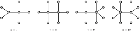
Figure 2.1: The trees with maximum value of $I_{f^{n}_{2}}(T)$ among all trees with $n$ vertices for $7\leq n\leq 10$.

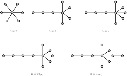
Figure 2.2: The trees with minimum value of $I_{f^{n}_{2}}(T)$ among all trees with $n$ vertices for $7\leq n\leq 10$.

2.7 Extremality of $I_{f^{\lambda}}(G)$, $I_{f^{2}}(G)$ $I_{f^{3}}(G)$ and entropy bounds for dendrimers

In the setting of information-theoretic graph measures, we will often consider a tuple $(\lambda_{1},\lambda_{2},\cdots,\lambda_{k})$ of nonnegative integers $\lambda_{i}\in N$. Let $G=(V,E)$ be a connected graph with $|V|=n$ vertices. Here, we define $f^{\lambda}(v_{i})=\lambda_{i}$, for all $v_{i}\in V$. Next we define $f^{2},f^{3}$ as follows.

Definition 2.18

[46] Let $G=(V,E)$. For a vertex $v_{i}\in V$, we define

$$f^{2}(v_{i}) := c_{1}|S_{1}(v_{i},G)|+c_{2}|S_{2}(v_{i},G)|+\cdots+c_{\rho}|S_{\rho}(v_{i},G)|,$$

$$c_{k}>0,\ 1\leq k\leq\rho,\ \alpha>0,$$

$$f^{3}(v_{i}) := c_{i}\sigma(v_{i}),\quad c_{k}>0,\ 1\leq k\leq n,$$

where $\sigma(v)$ and $S_{j}(v,G)$ are the eccentricity and the $j$-sphere of vertex $v$, respectively.

For the information function $f^{2}$, by applying the Equations 1.3 and 1.4 in Definition 1.8, we can obtain the following two entropy measures $I_{f^{2}}(G)$ and $I_{f^{2}}^{\lambda}(G)$.

$$I_{f^{2}}(G) := -\sum\limits_{i=1}^{|V|}\frac{f^{2}(v_{i})}{\sum_{j=1}^{|V|}f^{2}(v_{j})}\log\frac{f^{2}(v_{i})}{\sum_{j=1}^{|V|}f^{2}(v_{j})},$$

$$I_{f^{2}}^{\lambda}(G) := \lambda\left(\log(|V|)+\sum\limits_{i=1}^{|V|}\frac{f^{2}(v_{i})}{\sum_{j=1}^{|V|}f^{2}(v_{j})}\log\frac{f^{2}(v_{i})}{\sum_{j=1}^{|V|}f^{2}(v_{j})}\right).$$

In [11], the authors proved that if the graph $G=(V,E)$ is $k$-regular, then $I_{f^{2}}(G)=\log(|V|)$ and, hence, $I_{f^{2}}^{\lambda}(G)=0$.

For our purpose, we will mainly use decreasing sequences $c_{1},\cdots,c_{\rho(G)}$ of
(1)  constant decrease: $c_{1}:=S,c_{2}:=S-k,\cdots,c_{\rho(G)}:=S-(\rho(G)-1)k$,
(2)  quadratic decrease: $c_{1}:=S^{2},c_{2}:=(S-k)^{2},\cdots,c_{\rho(G)}:=(S-(\rho(G)-1)k)^{2}$,
(3)  exponential decrease: $c_{1}:=S,c_{2}:=Se^{-k},\cdots,c_{\rho(G)}:=Se^{-(\rho(G)-1)k}$.
Intuitive choices for the parameters are $S=\rho(G)$ and $k=1$.

Applying the Equation 1.3 in Definition 1.8, we can obtain three graph entropies as follows.

$$I(\lambda_{1},\lambda_{2},\cdots,\lambda_{n})=I_{f^{\lambda}}(G) = -\sum\limits_{i=1}^{n}\frac{\lambda_{i}}{\sum_{j=1}^{n}\lambda_{j}}\log\frac{\lambda_{i}}{\sum_{j=1}^{n}\lambda_{j}},$$

$$I_{f^{2}}(G) = -\sum\limits_{i=1}^{n}\frac{f^{2}(v_{i})}{\sum_{j=1}^{n}f^{2}(v_{j})}\log\frac{f^{2}(v_{i})}{\sum_{j=1}^{n}f^{2}(v_{j})},$$

$$I_{f^{3}}(G) = -\sum\limits_{i=1}^{n}\frac{f^{3}(v_{i})}{\sum_{j=1}^{n}f^{3}(v_{j})}\log\frac{f^{3}(v_{i})}{\sum_{j=1}^{n}f^{3}(v_{j})}.$$

As described in Definition 1.7, $p_{i}:=p^{f^{\lambda}}(v_{i})=\frac{\lambda_{i}}{\sum_{j=1}^{n}\lambda_{j}},\ i=1,2,\cdots,n$. We call $p=(p_{1},p_{2},\cdots,p_{n})$ be the probability distribution vector. Depending on probability distribution vector, we denote the entropy $I_{f^{\lambda}}(G)$ as $I_{p}(G)$ as well. Now we present some extremal properties of the entropy measure $I_{f^{\lambda}}(G)$, i.e., $I(\lambda_{1},\lambda_{2},\cdots,\lambda_{n})$.

Lemma 2.47

[46] If

(i)  $\lambda_{m}+x\leq\frac{\Sigma_{m}}{n-1}$ and $x\geq 0$, or

(ii)  $(\lambda_{m}+x)\Sigma_{m}\geq\sum_{i\in\{1,\cdots,n\}-m}\lambda_{i}^{2}$ and $-\lambda_{m}<x<0$,

then

$$I(\lambda_{1},\cdots,\lambda_{m-1},\lambda_{m},\lambda_{m+1},\cdots,\lambda_{n})\leq I(\lambda_{1},\cdots,\lambda_{m-1},\lambda_{m}+x,\lambda_{m+1},\cdots,\lambda_{n});$$

on the other hand, if

(iii)  $\lambda_{m}\leq\frac{\Sigma_{m}}{n-1}$ and $-\lambda_{m}<x<0$, or

(iv)  $\lambda_{m}\Sigma_{m}\geq\sum_{i\in\{1,\cdots,n\}-m}\lambda_{i}^{2}$ and $x>0$,

then

$$I(\lambda_{1},\cdots,\lambda_{m-1},\lambda_{m},\lambda_{m+1},\cdots,\lambda_{n})\geq I(\lambda_{1},\cdots,\lambda_{m-1},\lambda_{m}+x,\lambda_{m+1},\cdots,\lambda_{n}),$$

where $x\geq-\lambda_{m}$, $\Sigma=\sum_{j=1}^{n}\lambda_{j}$ and $\Sigma_{m}=\sum_{j\in\{1,\cdots,n\}-m}\lambda_{j}$.

Let $p=(p_{1},p_{2},\cdots,p_{n})$ be the original probability distribution vector and $\bar{p}=(\bar{p}_{1},\bar{p}_{2},\cdots,\bar{p}_{n})$ be the changed one, both ordered in increasing order. Further, let $\Delta p=\bar{p}-p=(\delta_{1},\cdots,\delta_{n})$ where $\delta_{1},\cdots,\delta_{n}\in\mathbb{R}$. Obviously, $\sum_{i=1}^{n}\delta_{i}=0$.

Lemma 2.48

[46] If

(i)  there exists a $k$ such that for all $1\leq i\leq k$, $\delta_{i}\leq 0$ and for all $k+1\leq i\leq n$, $\delta_{i}\geq 0$ or, more generally, if

(ii)  $\sum_{i=1}^{\ell}\delta_{i}\leq 0$ for all $\ell=1,\cdots,n$,

then

$$I_{\bar{p}}(G)\leq I_{p}(G).$$

Lemma 2.49

[46] For two probability distribution vectors $\bar{p}$ and $p$ fulfilling condition (ii) of Lemma 2.48, we have

$$I_{p}(G)-I_{\bar{p}}(G)\geq\sum\limits_{i=1}^{n}\delta_{i}\log p_{i}$$

where $\delta_{i}$ are the entries of $\Delta p=\bar{p}-p$.

Lemma 2.50

[46] Assume that for two probability distribution vectors $p$ and $\bar{p}$, the opposite of condition (ii) in Lemma 2.48 is true, that is $\sum_{i=\ell}^{n}\delta_{i}\geq 0$ for all $\ell=1,\cdots,n$. Then

$$0>I_{p}(G)-I_{\bar{p}}(G)\geq\sum\limits_{i:\delta_{i}<0}\delta_{i}\log(p_{i}-\rho)+\sum\limits_{i:\delta_{i}>0}\delta_{i}\log(p_{i}+\rho)$$

where $\rho=max_{i\in\{2,\cdots,n\}}(p_{i}-p_{i-1})$.

Proposition 2.51

[46] For two probability distribution vectors $p$ and $\bar{p}$ with $\sum_{i=1}^{\ell}\delta_{i}\leq 0$ for all $\ell$ in $\{0,\cdots,\ell_{1}-1\}\cup\{\ell_{2},\cdots,n\}\ (1\leq\ell_{1}<\ell_{2}\leq n)$, we have that

$$I_{p}(G)-I_{\bar{p}}(G) \geq \sum\limits_{i=1}^{\ell_{1}-1}\delta_{i}\log p_{i}+\sum\limits_{i=\ell_{2}}^{n}\delta_{i}\log p_{i}+\sum\limits_{i=\ell_{1}}^{\ell_{2}-1}\delta_{i}\log(p_{i}+\rho)$$

$$+\sum\limits_{i=1}^{\ell_{1}-1}\delta_{i}\log\left(\frac{p_{\ell_{1}}-\rho}{p_{\ell_{1}}}\right)+\sum\limits_{i=1}^{\ell_{2}-1}\delta_{i}\log\left(\frac{p_{\ell_{2}}}{p_{\ell_{2}}+\rho}\right)$$

where $\rho=max_{i\in\{2,\cdots,n\}}(p_{i}-p_{i-1})$. Hence, if

$$\sum\limits_{i=1}^{\ell_{1}-1}\delta_{i}\log p_{i}+\sum\limits_{i=\ell_{2}}^{n}\delta_{i}\log p_{i} \geq -\left(\sum\limits_{i=\ell_{1}}^{\ell_{2}-1}\delta_{i}\log(p_{i}+\rho)+\sum\limits_{i=1}^{\ell_{1}-1}\delta_{i}\log\left(\frac{p_{\ell_{1}}-\rho}{p_{\ell_{1}}}\right)\right.$$

$$\left.+\sum\limits_{i=1}^{\ell_{2}-1}\delta_{i}\log\left(\frac{p_{\ell_{2}}}{p_{\ell_{2}}+\rho}\right)\right),$$

it follows that

$$I_{p}(G)\geq I_{\bar{p}}(G).$$

In the following, we will show some results [42, 46] regarding the maximum and minimum entropy by using certain families of graphs.

As in every tree, a dendrimer has one (monocentric dendrimer) or two (dicentric dendrimer) central vertices, the radius $r$ denotes the (largest) distance from an external vertex to the (closer) center. If all external vertices are at distance $r$ from the center, the dendrimer is called homogeneous. Internal vertices different from the central vertices are called branching nodes and are said to be on the $i$-th orbit if their distance to the (nearer) center is $r$.

Let $D_{n}$ denote a homogeneous dendrimer on $n$ vertices with radius $r$ and progressive degree $p$, and let $z$ be its (unique) center. Further denote by $V_{i}(D_{n})$ the set of vertices in the $i$-th orbit. Now we consider the function $f^{3}(v_{i})=c_{i}\sigma(v_{i})$, where $c_{i}=c_{j}$ for $v_{i},v_{j}\in V_{i}$. We denote $\bar{c}_{i}=c(v),\ v\in V_{i}$.

Lemma 2.52

[46] For $\bar{c}_{i}=1$ with $i=0,\cdots,n$, the entropy fulfills

$$\log n-\frac{1}{4\ln 2}\leq I_{f^{3}}(D_{n})\leq\log n.$$

For $\bar{c}_{i}=r-i+1$ with $i=0,\cdots,n$, we have

$$\log n-\frac{(r-1)^{2}}{4\ln 2(r+1)}\leq I_{f^{3}}(D_{n})=\log n.$$

In general, for weight sequence $\bar{c}(i)$, $i=0,\cdots,r$, where $c(i)(r+i)$ is monotonic in $i$, we have

$$\log n-\frac{(\rho-1)^{2}}{2\rho\ln 2}\leq I_{f^{3}}(D_{n})\leq\log n$$

where $\rho=\frac{c(1)}{2c(r)}$ for decreasing and $\rho=\frac{2c(r)}{c(1)}$ for increasing sequences. The latter estimate is also true for any sequence $c(i)$, when $\rho=\frac{max_{i}(c(i)(r+i))}{min_{j}(c(j)(r+j))}$.

Lemma 2.53

[46] For dendrimers, the entropy $I_{f^{3}}(D_{n})$ is of order $\log n$ as $n$ tends to infinity.

By performing numerical experiments, Dehmer and Kraus [46] raised the following conjecture and also gave some ideas on how to prove it.

Conjecture 2.54

[46] Let $D$ be a dendrimer on $n$ vertices. For all sequences $\bar{c}_{0}\geq\bar{c}_{1}\geq\cdots\geq\bar{c}_{r}$, the star graph ($r=1,p=n-2$) have maximal and the path graph ($r=\lceil n-1/2\rceil,p=1$) have minimal values of entropy $I_{f^{3}}(D)$.

Additionally, in [42], the authors proposed another conjecture which is stated as follows.

Conjecture 2.55

[42] Let $D$ be a dendrimer on $n$ vertices. For all sequences $c_{i}=c_{j}$ with $i\neq j$, the star graph ($r=1,p=n-2$) has the minimal value of entropy $I_{f^{3}}(D)$.

Let $G$ be a generalized tree with hight $h$ which is defined as in Section 2.4. Denote by $|V|$ and $|V_{i}|$ the total number of vertices and the number of vertices on the $i$-th level, respectively. A probability distribution based on the vertices of $G$ is assigned as follows:

$$p_{i}^{V^{\prime}}=\frac{|V_{i}|}{|V|-1}.$$

Then another entropy of a generalized tree $G$ is defined by

$$I^{V^{\prime}}(G)=-\sum\limits_{i=1}^{h}p_{i}^{V^{\prime}}\log(p_{i}^{V^{\prime}}).$$

Similarly, denote by $|E|$ and $|E_{i}|$ the total number of edges and the number of edges on the $i$-th level, respectively. A probability distribution based on the edges of $G$ is assigned as follows:

$$p_{i}^{E^{\prime}}=\frac{|E_{i}|}{|E|-1}.$$

Then another entropy of a generalized tree $G$ is defined by

$$I^{E^{\prime}}(G)=-\sum\limits_{i=1}^{h}p_{i}^{E^{\prime}}\log(p_{i}^{E^{\prime}}).$$

Now we give some extremal properties [42] of $I^{V^{\prime}}(D)$ and $I^{E^{\prime}}(D)$, where $D$ is a dendrimer.

Theorem 2.56

[42] Let $D$ be a dendrimer on $n$ vertices. The star graph attains the minimal value of $I^{V^{\prime}}(D)$ and $I^{E^{\prime}}(D)$, and the dendrimer with parameter $t=t_{0}$ attains the maximal value of $I^{V^{\prime}}(D)$ and $I^{E^{\prime}}(D)$, where $t=t_{0}\in(1,n-2)$ is the integer which is closest to the root of the equation

$$\frac{n}{n-1}\ln\left(\frac{nt-n+2}{t+1}\right)-\ln\left(\frac{t(t+1)}{n-1}\right)-\frac{2t}{t+1}=0.$$

According to Rashevsky [1], $|X_{i}|$ denotes the number of topologically equivalent vertices in the $i$-th vertex orbit of $G$, where $k$ is the number of different orbits. Suppose $|X|=|V|-1$. Then the probability of $X_{i}$ can be expressed as $p_{i}^{V^{\prime}}=\frac{|V_{i}|}{|V|-1}$. Therefore, by applying Equations 1.9, 1.5, 1.7 in Definition 1.10, we can obtain the entropies as follows:

$$(i) \ I^{5}(G):=\sum\limits_{i=1}^{k}p_{i}^{V^{\prime}}(1-p_{i}^{V^{\prime}}),$$

$$(ii) \ I^{1}_{\alpha}(G):=\frac{1}{1-\alpha}\log\left(\sum\limits_{i=1}^{k}\left(p_{i}^{V^{\prime}}\right)^{\alpha}\right),\ \alpha\neq 1,$$

$$(iii) \ I^{3}_{\alpha}(G):=\frac{\sum\limits_{i=1}^{k}\left(p_{i}^{V^{\prime}}\right)^{\alpha}-1}{2^{1-\alpha}-1},\ \alpha\neq 1.$$

Theorem 2.57

[42] Let $D$ be a dendrimer on $n$ vertices.

(i)  The star graph and path graph attain the minimal and maximal value of $I^{5}(D)$, respectively.

(ii)  For $\alpha\neq 1$, the star graph and path graph attain the minimal and maximal value of $I^{1}_{\alpha}(D)$, respectively.

(iii)  For $\alpha\neq 1$, the star graph and path graph attain the minimal and maximal value of $I^{3}_{\alpha}(D)$, respectively.

Next we describe the algorithm for uniquely decomposing a graph $G\in\mathcal{G}_{UC}$ into a set of undirected generalized trees [47].

Algorithm 3.1: A graph $G\in\mathcal{G}_{UC}$ with $|V|$ vertices can be locally decomposed into a set of generalized trees as follows: Assign vertex labels to all vertices from $1$ to $|V|$. These labels form the label set $L_{S}=\{1,\cdots,|V|\}$. Choose a desired height of the trees that is denoted by $h$. Choose an arbitrary label from $L_{S}$, e.g., $i$. The vertex with this label is the root vertex of a tree. Now, perform the following steps:

1. Calculate the shortest distance from the vertex $i$ to all other vertices in the graph $G$, e.g., by the algorithm of Dijkstra; see Dijkstra (1959).

2. The vertices with distance $k$ from the vertex $i$ are the vertices on the $k$-th level of the resulting generalized trees. Select all vertices of the graph up to distance $h$, including the connections between the vertices. Connections to vertices with distance $>h$ are deleted.

3. Delete the label $i$ from the label set $L_{S}$.

4. Repeat this procedure if $L_{S}$ is not empty by choosing an arbitrary label from $L_{S}$; otherwise terminate.

Now we replace $p_{i}^{E^{\prime}}=\frac{|E_{i}|}{|E|-1}$ by $p_{i}^{E^{\prime}}=\frac{|E_{i}|}{2|E|-d(r)}$, where $r$ is the root of the generalized tree and $d(r)$ is the degree of $r$. Then we can obtain a new $I^{E^{\prime}}(G)$ which is defined similarly as above. Additionally, we give another definition of the structural information content of a graph as follows.

Definition 2.19

[47] Let $G\in\mathcal{G}_{UC}$ and $S_{G}^{H}:=\{H_{1},H_{2},\cdots,H_{|V|}\}$ be the associated set of generalized trees obtained from Algorithm 3.1. We now define the structural information content of $G$ by

$$I^{V^{\prime}}(G):=-\sum\limits_{i=1}^{|V|}I^{V^{\prime}}(H_{i})$$

and

$$I^{E^{\prime}}(G):=-\sum\limits_{i=1}^{|V|}I^{E^{\prime}}(H_{i}).$$

In [47], Dehmer analyzed the time complexities for calculating the entropies $I^{V^{\prime}}(G)$ and $I^{E^{\prime}}(G)$ depending on the decomposition given by Algorithm 3.1.

Theorem 2.58

[47] The overall time complexity to calculate $I^{V^{\prime}}(G)$ and $I^{E^{\prime}}(G)$ is finally $O(|V|^{3}+\sum_{i=1}^{|V|}|V_{H_{i}}|^{2})$.

Let $T_{n,d}$ be the family of trees of order $n$ with a fixed diameter $d$. We call a tree consisting of a star on $n-d+1$ vertices together with a path of length $d-1$ attached to the central vertex, a comet of order $n$ with tail length $d-1$, and denote it by $C_{n,d-1}$. Analogously, we call a tree consisting of a star on $n-d$ vertices together with $2$ paths of lengths $\lfloor\frac{d}{2}\rfloor$ and $\lceil\frac{d}{2}\rceil$, respectively, attached to the central vertex, a two-tailed comet of order $n$ and denote it by $C_{n,\lfloor\frac{d}{2}\rfloor,\lceil\frac{d}{2}\rceil}$.

Theorem 2.59

[46] For every linearly or exponentially decreasing sequence $c_{1}>c_{2}>\cdots>c_{d}$ with $d\geq 4$ as well as every quadratically decreasing sequence with $d\geq 5$, for large enough $n$, the probability distribution $q(n,d)$ of the $2$-tailed comet $C_{n,\lfloor\frac{d}{2}\rfloor,\lceil\frac{d}{2}\rceil}$ is majorities by the probability distribution $p(n,d)$ of the comet $C_{n,d-1}$. This is equivalent to the fact that $\Delta p=q-p$ fulfills condition (ii) of Lemma 2.48. Hence,

$$I_{f^{2}}(C_{n,\lfloor\frac{d}{2}\rfloor,\lceil\frac{d}{2}\rceil})\geq I_{f^{2}}(C_{n,d-1}).$$

Conjecture 2.60

[46] Among all trees $T_{n,d}$, with $d<<n$, the $2$-tailed comet $C_{n,\lfloor\frac{n}{2}\rfloor,\lceil\frac{n}{2}\rceil}$ achieves maximal value of the entropies $I_{f^{2}}(G)$ and $I_{f^{3}}(G)$.

2.8 Sphere-regular graphs and the extremality entropies $I_{f^{2}}(G)$ and $I_{f^{\sigma}}(G)$

Let $G=(V,E)$ be a connected graph with $|V|=n$ vertices. As we have defined before, the information function $f^{2}(v_{i})=c_{1}|S_{1}(v_{i},G)|+c_{2}|S_{2}(v_{i},G)|+\cdots+c_{\rho}|S_{\rho}(v_{i},G)|$, where $c_{k}>0$, $1\leq k\leq\rho,\ \alpha>0$, and $S_{j}(v,G)$ is the $j$-sphere of the vertex $v$. Now we define another information function.

Definition 2.20

The eccentricity-function $f^{\sigma}$ if defined by

$$f^{\sigma}:\ V\rightarrow\mathbb{Z}:\quad f^{\sigma}(v)=\sigma(v).$$

Applying the Equation 1.3 in Definition 1.8, we can obtain the following two graph entropy measures [48].

$$I_{f^{2}}(G):=-\sum\limits_{i=1}^{n}\frac{f^{2}(v_{i})}{\sum_{j=1}^{n}f^{2}(v_{j})}\log\frac{f^{2}(v_{i})}{\sum_{j=1}^{n}f^{2}(v_{j})},$$

$$I_{f^{\sigma}}(G):=-\sum\limits_{i=1}^{n}\frac{f^{\sigma}(v_{i})}{\sum_{j=1}^{n}f^{\sigma}(v_{j})}\log\frac{f^{\sigma}(v_{i})}{\sum_{j=1}^{n}f^{\sigma}(v_{j})}.$$

In [48], the authors proposed the concept of sphere-regular.

Definition 2.21

[48] We call a graph sphere-regular if there exist positive integers $s_{1},\cdots,s_{\rho(G)}$, such that

$$(|S_{1}(v,G)|,|S_{2}(v,G)|,\cdots,|S_{\rho(G)}(v,G)|)=(s_{1},\cdots,s_{\rho(G)})$$

for all vertices $v\in V$.

In [48], the authors also tried to classify those graphs which return maximal value of entropy $I_{f^{2}}(G)$ for the sphere-function and an arbitrary decreasing weight sequence. In the following, we state their results.

Proposition 2.61

[48] Every sphere-regular graph with $n$ vertices has maximum entropy $I_{f^{2}}(G)=\log n$.

Lemma 2.62

[48] Sphere-regular graphs are the only maximal graphs for $I_{f^{2}}(G)$ when using a weight sequence such that there exist no numbers $a_{i},\ i=1,\cdots,\rho(G)$, $a_{i}\in\mathbb{Z}$ with $\sum_{i=1}^{\rho(G)}a_{i}=0$, where

$$\sum_{j=1}^{\rho(G)}a_{j}c_{j}=0.$$

Theorem 2.63

[48] There are maximal graphs with respect to $I_{f^{2}}(G)$ which are not sphere-regular.

Next, we will present some restrictions on maximal graphs for $I_{f^{2}}(G)$, which are valid for any decreasing weight sequence.

Lemma 2.64

[48] A graph of diameter $2$ is maximal for $I_{f^{2}}(G)$ if and only if it is sphere-regular.

Lemma 2.65

[48] Maximal graphs for $I_{f^{2}}(G)$ cannot have unary vertices (vertices with degree $1$). Hence, in particular, trees cannot be maximal for $I_{f^{2}}(G)$.

Corollary 2.66

[48] The last nonzero entries of the sphere-sequence of a vertex in a maximal graph cannot be $2$ or more consecutive ones.

Lemma 2.67

[48] A maximal graph for $I_{f^{2}}(G)$ different from the complete graph $K_{n}$ cannot contain a vertex of degree $n-1$.

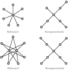
Figure 2.3: Minimal graphs for $I_{f^{2}}(G)$ of orders $8$ and $9$.

In [48], the authors gave the minimal graphs for $I_{f^{2}}(G)$ of orders $8$ and $9$ by computations, which are depicted in Figure 2.3. Its left graphs are minimal for the linear sequence and the right ones are minimal for the exponential sequence. Unfortunately, there is very little known about minimal entropy graphs. And the authors gave the following conjecture in [48].

Conjecture 2.68

[48] The minimal graph for $I_{f^{2}}(G)$ with the exponential sequence is a tree. Further it is a generalized star of diameter approximately $\sqrt{2n}$ and, hence, with approximately $\sqrt{2n}$ branches.

Interestingly, the graph $9(linear)$ is also one of the maximal graphs for $I_{f^{\sigma}}(G)$ in $N_{9}$, where $N_{i}$ is the set of all non-isomorphic graphs on $i$ vertices. In addition, one elementary result on maximal graphs with respect to $f^{\sigma}$ is also obtained.

Lemma 2.69

[48] (i) A graph $G$ is maximal with respect to $I_{f^{\sigma}}(G)$ if and only if its every vertex is an endpoint of a maximal path in $G$.

(ii) A maximal graph different from the complete graph $K_{n}$ cannot contain a vertex of degree $n-1$.

Similar to the case of $I_{f^{2}}(G)$, there is still very little known about minimal entropy graphs respect to $I_{f^{\sigma}}(G)$. For $N_{8}$ and $N_{9}$, computations show that there are $2$ minimal graphs. For $n=8$, they are depicted in Figure 2.4, for $n=9$ they contain $5$ vertices of degree $8$ each. The authors [48] gave another conjecture as follows.

Conjecture 2.70

[48] A minimal graph for $I_{f^{\sigma}}(G)$ is a highly connected graph, i.e., it is a graph obtained from the complete graph $K_{n}$ by removal of a small number of edges. In particular, we conjecture that a minimal graph for $I_{f^{\sigma}}(G)$ on $n$ vertices will have $m\geq\frac{n}{2}$ vertices of degree $n-1$.

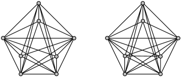
Figure 2.4: Minimal graphs for $I_{f^{\sigma}}(G)$ of order $8$.

2.9 Information inequalities for generalized graph entropies

Sivakumar and Dehmer [49] discussed the problem of establishing relations between information measures for network structures. Two types of entropy measures, namely, the Shannon entropy and its generalization, the Rényi entropy have been considered for their study. They established formal relationships, by means of inequalities, between these two kinds of measures. In addition, they proved inequalities connecting the classical partition-based graph entropies and partition-independent entropy measures, and also gave several explicit inequalities for special classes of graphs.

To begin with, we give the theorem which provide the bounds for Rényi entropy in terms of Shannon entropy.

Theorem 2.71

[49] Let $p^{f}(v_{1}),p^{f}(v_{2}),\cdots,p^{f}(v_{n})$ be the probability values on the vertices of a graph $G$ with $n$ vertices. Then the Rényi entropy can be bounded by the Shannon entropy as follows:
when $0<\alpha<1$,

$$I_{f}(G)\leq I^{2}_{\alpha}(G)_{f}<I_{f}(G)+\frac{n(n-1)(1-\alpha)\rho^{\alpha-2}}{2\ln 2},$$

when $\alpha>1$,

$$I_{f}(G)-\frac{(\alpha-1)n(n-1)}{2\ln 2\cdot\rho^{\alpha-2}}<I^{2}_{\alpha}(G)_{f}\leq I_{f}(G),$$

where $\rho=max_{i,k}\frac{p^{f}(v_{i})}{p^{f}(v_{k})}$.

Observe that Theorem 2.71, in general, holds for any probability distribution with non-zero probability values. The following theorem illustrates this fact with the help of a probability distribution obtained by partitioning a graph object.

Theorem 2.72

[49] Let $p_{1},p_{2},\cdots,p_{k}$ be the probabilities of the partitions obtained using an equivalence relation $\tau$ as stated before. Then
when $0<\alpha<1$,

$$I(G,\tau)\leq I^{1}_{\alpha}(G)<I(G,\tau)+\frac{k(k-1)(1-\alpha)\rho^{\alpha-2}}{2\ln 2},$$

when $\alpha>1$,

$$I(G,\tau)\geq I^{1}_{\alpha}(G)>I(G,\tau)-\frac{k(k-1)(\alpha-1)}{2\ln 2\cdot\rho^{\alpha-2}},$$

where $\rho=max_{i,j}\frac{p_{i}}{p_{j}}$.

In the next theorem, bounds between like-entropy measures are established, by considering the two different probability distributions.

Theorem 2.73

[49] Let $G$ be a graph with $n$ vertices. Suppose $|X_{i}|<f(v_{i})$ for $1\leq i\leq k$. Then

$$I^{1}_{\alpha}(G)<I^{2}_{\alpha}(G)_{f}+\frac{\alpha}{1-\alpha}\log_{2}\left(\frac{S}{|X|}\right)$$

if  $0<\alpha<1$, and

$$I^{1}_{\alpha}(G)>I^{2}_{\alpha}(G)_{f}-\frac{\alpha}{\alpha-1}\log_{2}\left(\frac{S}{|X|}\right)$$

if  $\alpha>1$. Here $S=\sum_{i=1}^{n}f(v_{i})$.

Furthermore, Sivakumar and Dehmer [49] also paid attention to generalized graph entropies which is inspired by the Rényi entropy, and presented various bounds when two different functions and their probability distributions satisfy certain initial conditions. Let $f_{1}$ and $f_{2}$ be two information functions defined on $G=(V,E)$ with $|V|=n$. Let $S_{1}=\sum_{i=1}^{n}f_{1}(v_{i})$ and $S_{2}=\sum_{i=1}^{n}f_{2}(v_{i})$. Let $p^{f_{1}}(v)$ and $p^{f_{2}}(v)$ denote the probabilities of $f_{1}$ and $f_{2}$, respectively, on a vertex $v\in V$.

Theorem 2.74

[49] Suppose $p^{f_{1}}(v)\leq\psi p^{f_{2}}(v)$, $\forall v\in V$ and $\psi>0$ a constant. Then,
if  $0<\alpha<1$,

$$I^{2}_{\alpha}(G)_{f_{1}}\leq I^{2}_{\alpha}(G)_{f_{2}}+\frac{\alpha}{1-\alpha}\log_{2}\psi,$$

and if  $\alpha>1$,

$$I^{2}_{\alpha}(G)_{f_{1}}\geq I^{2}_{\alpha}(G)_{f_{2}}-\frac{\alpha}{\alpha-1}\log_{2}\psi.$$

Theorem 2.75

[49] Suppose $p^{f_{1}}(v)\leq p^{f_{2}}(v)+\phi$, $\forall v\in V$ and $\phi>0$ a constant. Then,

$$I^{2}_{\alpha}(G)_{f_{1}}-I^{2}_{\alpha}(G)_{f_{2}}<\frac{1}{1-\alpha}\frac{n\cdot\phi^{\alpha}}{\sum\limits_{v\in V}\left(p^{f_{2}}(v)\right)^{\alpha}}$$

if  $0<\alpha<1$, and

$$I^{2}_{\alpha}(G)_{f_{2}}-I^{2}_{\alpha}(G)_{f_{1}}<\frac{\alpha}{\alpha-1}\frac{n^{\frac{1}{\alpha}}\cdot\phi}{\left(\sum\limits_{v\in V}\left(p^{f_{2}}(v)\right)^{\alpha}\right)^{\frac{1}{\alpha}}}$$

if  $\alpha>1$.

Theorem 2.76

[49] Let $f(v)=c_{1}f_{1}(v)+c_{2}f_{2}(v)$, $\forall v\in V$. Then
for $0<\alpha<1$,

$$I^{2}_{\alpha}(G)_{f}<I^{2}_{\alpha}(G)_{f_{1}}+\frac{\alpha}{1-\alpha}\log_{2}A_{1}+\frac{1}{1-\alpha}\frac{A^{\alpha}_{2}}{A^{\alpha}_{1}}\frac{\sum\limits_{v\in V}\left(p^{f_{2}}(v)\right)^{\alpha}}{\sum\limits_{v\in V}\left(p^{f_{1}}(v)\right)^{\alpha}},$$

and for $\alpha>1$,

$$I^{2}_{\alpha}(G)_{f}>I^{2}_{\alpha}(G)_{f_{1}}-\frac{\alpha}{\alpha-1}\log_{2}A_{1}-\frac{\alpha}{\alpha-1}\frac{A_{2}}{A_{1}}\left(\frac{\sum\limits_{v\in V}\left(p^{f_{2}}(v)\right)^{\alpha}}{\sum\limits_{v\in V}\left(p^{f_{1}}(v)\right)^{\alpha}}\right)^{\frac{1}{\alpha}},$$

where $A_{1}=\frac{c_{1}S_{1}}{c_{1}S_{1}+c_{2}S_{2}}$ and $A_{2}=\frac{c_{2}S_{2}}{c_{1}S_{1}+c_{2}S_{2}}$.

Theorem 2.77

[49] Let $f(v)=c_{1}f_{1}(v)+c_{2}f_{2}(v)$, $\forall v\in V$. Then
if  $0<\alpha<1$,

$$I^{2}_{\alpha}(G)_{f} < \frac{1}{2}\left[I^{2}_{\alpha}(G)_{f_{1}}+I^{2}_{\alpha}(G)_{f_{2}}\right]+\frac{\alpha}{2(1-\alpha)}\log_{2}(A_{1}A_{2})$$

$$+\frac{1}{2(1-\alpha)}\left[\frac{A^{\alpha}_{2}}{A^{\alpha}_{1}}\frac{\sum\limits_{v\in V}\left(p^{f_{2}}(v)\right)^{\alpha}}{\sum\limits_{v\in V}\left(p^{f_{1}}(v)\right)^{\alpha}}+\frac{A^{\alpha}_{1}}{A^{\alpha}_{2}}\frac{\sum\limits_{v\in V}\left(p^{f_{1}}(v)\right)^{\alpha}}{\sum\limits_{v\in V}\left(p^{f_{2}}(v)\right)^{\alpha}}\right],$$

and if  $\alpha>1$,

$$I^{2}_{\alpha}(G)_{f} > \frac{1}{2}\left[I^{2}_{\alpha}(G)_{f_{1}}+I^{2}_{\alpha}(G)_{f_{2}}\right]-\frac{\alpha}{2(\alpha-1)}\log_{2}(A_{1}A_{2})$$

$$-\frac{\alpha}{2(\alpha-1)}\left[\frac{A_{2}}{A_{1}}\left(\frac{\sum\limits_{v\in V}\left(p^{f_{2}}(v)\right)^{\alpha}}{\sum\limits_{v\in V}\left(p^{f_{1}}(v)\right)^{\alpha}}\right)^{\frac{1}{\alpha}}+\frac{A_{1}}{A_{2}}\left(\frac{\sum\limits_{v\in V}\left(p^{f_{1}}(v)\right)^{\alpha}}{\sum\limits_{v\in V}\left(p^{f_{2}}(v)\right)^{\alpha}}\right)^{\frac{1}{\alpha}}\right],$$

where $A_{1}=\frac{c_{1}S_{1}}{c_{1}S_{1}+c_{2}S_{2}}$ and $A_{2}=\frac{c_{2}S_{2}}{c_{1}S_{1}+c_{2}S_{2}}$.

Let $S_{n}$ be a star on $n$ vertices whose central vertex is denoted by $u$. Let $\tau$ be an automorphism defined on $S_{n}$ such that $\tau$ partitions $V(S_{n})$ into two orbits, $V_{1}$ and $V_{2}$, where $V_{1}=\{u\}$ and $V_{2}=V(S_{n})-\{u\}$.

Theorem 2.78

[49] If $\tau$ is the automorphism, as defined above, on $S_{n}$, then
for $0<\alpha<1$,

$$I^{1}_{\alpha}(S_{n})<\log_{2}n-\frac{n-1}{n}\log_{2}(n-1)+\frac{(1-\alpha)(n-1)^{\alpha-2}}{\ln 2},$$

and for $\alpha>1$,

$$I^{1}_{\alpha}(S_{n})>\log_{2}n-\frac{n-1}{n}\log_{2}(n-1)-\frac{\alpha-1}{(n-1)^{\alpha-2}\ln 2}.$$

Theorem 2.79

[49] Let $\tau$ be an automorphism on $V(S_{n})$ and let $f$ be any information function defined on $V(S_{n})$ such that $|V_{1}|<f(v_{i})$ and $|V_{2}|<f(v_{j})$ for some $i,j$, $1\leq i\neq j\leq n$. Then
for $0<\alpha<1$,

$$I^{2}_{\alpha}(S_{n})_{f}>\frac{1}{1-\alpha}\log_{2}(1+(n-1)^{\alpha})-\frac{\alpha}{1-\alpha}\log_{2}S,$$

and for $\alpha>1$,

$$I^{2}_{\alpha}(S_{n})_{f}<\frac{1}{1-\alpha}\log_{2}(1+(n-1)^{\alpha})+\frac{\alpha}{\alpha-1}\log_{2}S,$$

where $S=\sum_{v\in V}f(v)$.

The path graph, denoted by $P_{n}$, are the only trees with maximum diameter among all the trees on $n$ vertices. Let $\tau$ be an automorphism defined on $P_{n}$, where $\tau$ partitions the vertices of $P_{n}$ into $\frac{n}{2}$ orbits $(V_{i})$ of size $2$, when $n$ is even, and $\frac{n-1}{2}$ orbits of size $2$ and one orbit of size $1$, when $n$ is odd. Sivakumar and Dehmer [49] derived equalities and inequalities on generalized graph entropies $I^{1}_{\alpha}(P_{n})$ and $I^{2}_{\alpha}(P_{n})_{f}$ depending on the parity of $n$.

Theorem 2.80

[49] Let $n$ be an even integer and $f$ be any information function such that $f(v)>2$ for at least $\frac{n}{2}$ vertices of $P_{n}$ and let $\tau$ be stated as above. Then

$$I^{1}_{\alpha}(P_{n})=\log_{2}\frac{n}{2},$$

and

$$I^{2}_{\alpha}(P_{n})_{f}>\frac{1}{1-\alpha}\log_{2}n-\frac{\alpha}{1-\alpha}\log_{2}S-1$$

if  $0<\alpha<1$,

$$I^{2}_{\alpha}(P_{n})_{f}<\frac{1}{1-\alpha}\log_{2}n+\frac{\alpha}{\alpha-1}\log_{2}S-1$$

if  $\alpha>1$, where $S=\sum_{v\in V}f(v)$.

Theorem 2.81

[49] Let $n$ be an odd integer and $\tau$ be defined as before. Then
when $0\leq\alpha<1$,

$$\log_{2}n-\frac{n-1}{n}\leq I^{1}_{\alpha}(P_{n})<\log_{2}n+(n-1)\left[\frac{(n+1)\cdot(1-\alpha)}{\ln 2\cdot 2^{5-\alpha}}-\frac{1}{n}\right],$$

and when $\alpha>1$,

$$\log_{2}n-\frac{n-1}{n}\geq I^{1}_{\alpha}(P_{n})>\log_{2}n-(n-1)\left[\frac{(n+1)\cdot(\alpha-1)}{\ln 2\cdot 2^{\alpha+1}}+\frac{1}{n}\right].$$

Further if $f$ is an information function such that $f(v)>2$ for at least $\frac{n+1}{2}$ vertices of $P_{n}$, then

$$I^{2}_{\alpha}(P_{n})_{f}>\frac{1}{1-\alpha}\log_{2}n-\frac{\alpha}{1-\alpha}\log_{2}S-\frac{n-1}{n}$$

if  $0<\alpha<1$, and

$$I^{2}_{\alpha}(P_{n})_{f}<\frac{1}{1-\alpha}\log_{2}n+\frac{\alpha}{\alpha-1}\log_{2}S-\frac{n-1}{n}$$

if  $\alpha>1$, where $S=\sum_{v\in V}f(v)$.

In [49], Sivakumar and Dehmer derived bounds of generalized graph entropy $I^{2}_{\alpha}(G)_{f}$ for not only special graph classes but also special information functions. Let $G=(V,E)$ be a simple undirected graph on $n$ vertices and let $d(u,v)$, $S_{j}(u,G)$ be the distance between $u,v$ and the $j$-sphere of $u$, respectively. For the two special information functions $f_{P}(v_{i})$ and $f_{P^{\prime}}(v_{i})$, Sivakumar and Dehmer [49] presented the explicit bounds for the graph entropy measures $I^{2}_{\alpha}(G)_{f_{P}}$ and $I^{2}_{\alpha}(G)_{f_{P^{\prime}}}$.

Theorem 2.82

[49] Let $f_{P}$ be given by equation 2.14. Let $c_{max}=max\{c_{i}:1\leq i\leq\rho(G)\}$ and $c_{min}=min\{c_{i}:1\leq i\leq\rho(G)\}$ where $c_{i}$ is defined in $f_{P}$. Then the value of $I^{2}_{\alpha}(G)_{f_{P}}$ can be bounded as follows.
If  $0<\alpha<1$,

$$\log_{2}n-\frac{\alpha(n-1)X}{1-\alpha}\log_{2}\beta\leq I^{2}_{\alpha}(G)_{f_{P}}\leq\log_{2}n+\frac{\alpha(n-1)X}{1-\alpha}\log_{2}\beta,$$

and if  $\alpha>1$,

$$\log_{2}n-\frac{\alpha(n-1)X}{\alpha-1}\log_{2}\beta\leq I^{2}_{\alpha}(G)_{f_{P}}\leq\log_{2}n+\frac{\alpha(n-1)X}{\alpha-1}\log_{2}\beta,$$

where $X=c_{max}-c_{min}$.

Theorem 2.83

[49] Let $f_{P^{\prime}}$ be given by equation 2.15. Let $c_{max}=max\{c_{i}:1\leq i\leq\rho(G)\}$ and $c_{min}=min\{c_{i}:1\leq i\leq\rho(G)\}$ where $c_{i}$ is defined in $f_{P^{\prime}}$. Then the value of $I^{2}_{\alpha}(G)_{f_{P^{\prime}}}$ can be bounded as follows.
If  $0<\alpha<1$,

$$\log_{2}n-\frac{\alpha}{1-\alpha}\log_{2}Y\leq I^{2}_{\alpha}(G)_{f_{P^{\prime}}}\leq\log_{2}n+\frac{\alpha}{1-\alpha}\log_{2}Y,$$

and if  $\alpha>1$,

$$\log_{2}n-\frac{\alpha}{\alpha-1}\log_{2}Y\leq I^{2}_{\alpha}(G)_{f_{P^{\prime}}}\leq\log_{2}n+\frac{\alpha}{\alpha-1}\log_{2}Y,$$

where $Y=\frac{c_{max}}{c_{min}}$.

3 Relationships between graph structures, graph energies, topological indices and generalized graph entropies

In this section, we introduce ten generalized graph entropies based on distinct graph matrices. Connections between such generalized graph entropies and the graph energies, the spectral moments and topological indices are provided. Moreover, we will give some extremal properties of these generalized graph entropies and several inequalities between them.

Let $G$ be a graph of order $n$ and $M$ be a matrix related to the graph $G$. Denote $\mu_{1},\mu_{2},\cdots,\mu_{n}$ be the eigenvalues of $M$ (or the singular values for some matrices). If $f:=|\mu_{i}|$, then as defined in Definition 1.7,

$$p^{f}(v_{i})=\frac{|\mu_{i}|}{\sum\limits_{j=1}^{n}|\mu_{j}|}.$$

Therefore, the generalized graph entropies are defined as follows:

$$(i) \ I^{6}(G)_{\mu}=\sum_{i=1}^{n}\frac{|\mu_{i}|}{\sum\limits_{j=1}^{n}|\mu_{j}|}\left[1-\frac{|\mu_{i}|}{\sum\limits_{j=1}^{n}|\mu_{j}|}\right],$$

$$(ii) \ I^{2}_{\alpha}(G)_{\mu}=\frac{1}{1-\alpha}\log\left(\sum_{i=1}^{n}\left(\frac{|\mu_{i}|}{\sum\limits_{j=1}^{n}|\mu_{j}|}\right)^{\alpha}\right),\quad\alpha\neq 1,$$

$$(iii) \ I^{4}_{\alpha}(G)_{\mu}=\frac{1}{2^{1-\alpha}-1}\left(\sum\limits_{i=1}^{n}\left(\frac{|\mu_{i}|}{\sum\limits_{j=1}^{n}|\mu_{j}|}\right)^{\alpha}-1\right),\quad\alpha\neq 1.$$

1. Let $A(G)$ be the adjacency matrix of graph $G$ and the eigenvalues of $A(G)$, $\lambda_{1},\lambda_{2},\cdots,\lambda_{n}$, are said to be the eigenvalues of the graph $G$. The energy of $G$ is $\varepsilon(G)=\sum_{i=1}^{n}|\lambda_{i}|$. The $k$-th spectral moment of the graph $G$ is defined as $M_{k}(G)=\sum_{i=1}^{n}\lambda_{i}^{k}$. In [50], the authors defined the moment-like quantities, $M^{*}_{k}(G)=\sum_{i=1}^{n}|\lambda_{i}|^{k}$.

Theorem 3.1

[51] Let $G$ be a graph with $n$ vertices and $m$ edges. Then for $\alpha\neq 1$, we have

$$(i) \ I^{6}(G)_{\lambda}=1-\frac{2m}{\varepsilon^{2}},$$

$$(ii) \ I_{\alpha}^{2}(G)_{\lambda}=\frac{1}{1-\alpha}\log\frac{M_{\alpha}^{*}}{\varepsilon^{\alpha}},$$

$$(iii) \ I_{\alpha}^{4}(G)_{\lambda}=\frac{1}{2^{1-\alpha}-1}\left(\frac{M_{\alpha}^{*}}{\varepsilon^{\alpha}}-1\right),$$

where $\varepsilon$ denotes the energy of graph $G$ and $M_{\alpha}^{*}=\sum\limits_{i=1}^{n}|\lambda_{i}|^{\alpha}$.

The above theorem directly implies that for a graph $G$, each upper (lower) bound of energy can be used to deduce an upper (a lower) bound of $I^{6}(G)_{\lambda}$.

Corollary 3.2

[51]

(i)   For a graph $G$ with $m$ edges, we have

$$\frac{1}{2}\leq I^{6}(G)_{\lambda}\leq 1-\frac{1}{2m}.$$

(ii)   Let $G$ be a graph with $n$ vertices and $m$ edges. Then

$$I^{6}(G)_{\lambda}\leq 1-\frac{1}{n}.$$

(iii)  Let $T$ be a tree of order $n$. We have

$$I^{6}(S_{n})_{\lambda}\leq I^{6}(T)_{\lambda}\leq I^{6}(P_{n})_{\lambda},$$

where $S_{n}$ and $P_{n}$ denote the star graph and path graph of order $n$, respectively.

(iv)  Let $G$ be a unicyclic graph of order $n$. Then we have

$$I^{6}(G)_{\lambda}\leq I^{6}(P_{n}^{6})_{\lambda},$$

where $P_{n}^{6}$ [52, 53] denotes the unicyclic graph obtained by connecting a vertex of $C_{6}$ with a leaf of order $P_{n-6}$, respectively.

(v)  Let $G$ be a graph with $n$ vertices and $m$ edges. If its cyclomatic number is $k=m-n+1$, then we have

$$I^{6}(G)_{\lambda}\leq 1-\frac{2m}{(4n/\pi+c_{k})^{2}},$$

where $c_{k}$ is a constant which only depends on $k$.

2. Let $Q(G)$ be the signless Laplacian matrix of a graph $G$. Then $Q(G)=D(G)+A(G)$, where $D(G)={\rm diag}(d_{1},d_{2},\cdots,d_{n})$ denotes the diagonal matrix of vertex degrees of $G$ and $A(G)$ is the adjacency matrix of $G$. Let $q_{1},q_{2},\cdots,q_{n}$ be the eigenvalues of $Q(G)$.

Theorem 3.3

[54] Let $G$ be a graph with $n$ vertices and $m$ edges. Then for $\alpha\neq 1$, we have

$$(i) \ I^{6}(G)_{q}=1-\frac{1}{4m^{2}}(M_{1}+2m),$$

$$(ii) \ I_{\alpha}^{2}(G)_{q}=\frac{1}{1-\alpha}\log\frac{M_{\alpha}^{*}}{(2m)^{\alpha}},$$

$$(iii) \ I_{\alpha}^{4}(G)_{q}=\frac{1}{2^{1-\alpha}-1}\left(\frac{M_{\alpha}^{*}}{(2m)^{\alpha}}-1\right),$$

where $M_{1}$ denotes the first Zagreb index and $M_{\alpha}^{*}=\sum\limits_{i=1}^{n}|q_{i}|^{\alpha}$.

Corollary 3.4

[54]

(i)  For a graph $G$ with $n$ vertices and $m$ edges, we have

$$I^{6}(G)_{q}\leq 1-\frac{1}{2m}-\frac{1}{n}.$$

(ii)  Let $G$ be a graph with $n$ vertices and $m$ edges. The minimum degree of $G$ is $\delta$ and the maximum degree of $G$ is $\Delta$. Then

$$I^{6}(G)_{q}\geq 1-\frac{1}{2m}-\frac{1}{2n}-\frac{\Delta^{2}+\delta^{2}}{4n\Delta\delta},$$

with equality if and only if $G$ is a regular graph, or $G$ is a graph whose vertices have exactly two degrees $\Delta$ and $\delta$ such that $\Delta+\delta$ divides $\delta n$ and there are exactly $p=\frac{\delta n}{\delta+\Delta}$ vertices of degree $\Delta$ and $q=\frac{\Delta n}{\delta+\Delta}$ vertices of degree $\delta$.

3. Let $\mathscr{L}(G)$ and $\mathcal{Q}(G)$ be the normalized Laplacian matrix and the normalized signless Laplacian matrix, respectively. By definition, $\mathscr{L}(G)=D(G)^{-\frac{1}{2}}L(G)D(G)^{-\frac{1}{2}}$ and $\mathcal{Q}(G)=D(G)^{-\frac{1}{2}}Q(G)D(G)^{-\frac{1}{2}}$, where $D(G)$ is the diagonal matrix of vertex degrees, and $L(G)=D(G)-A(G)$, $Q(G)=D(G)+A(G)$ are, respectively, the Laplacian and the signless Laplacian matrices of the graph $G$. Denote the eigenvalues of $\mathscr{L}(G)$ and $\mathcal{Q}(G)$ by $\mu_{1},\mu_{2},\cdots,\mu_{n}$ and $q_{1},q_{2},\cdots,q_{n}$, respectively.

Theorem 3.5

[54] Let $G$ be a graph with $n$ vertices and $m$ edges. Then for $\alpha\neq 1$, we have

$$(i) \ I^{6}(G)_{\mu}=I^{6}(G)_{q}=1-\frac{1}{n^{2}}(n+2R_{-1}(G)),$$

$$(ii) \ I_{\alpha}^{2}(G)_{\mu}=\frac{1}{1-\alpha}\log\frac{M_{\alpha}^{*}}{n^{\alpha}},\ \ I_{\alpha}^{2}(G)_{q}=\frac{1}{1-\alpha}\log\frac{M_{\alpha}^{*^{\prime}}}{n^{\alpha}},$$

$$(iii) \ I_{\alpha}^{4}(G)_{\mu}=\frac{1}{2^{1-\alpha}-1}\left(\frac{M_{\alpha}^{*}}{n^{\alpha}}-1\right),\ \ I_{\alpha}^{4}(G)_{q}=\frac{1}{2^{1-\alpha}-1}\left(\frac{M_{\alpha}^{*^{\prime}}}{n^{\alpha}}-1\right),$$

where $R_{-1}(G)$ denotes the general Randić index $R_{\beta}(G)$ of $G$ with $\beta=-1$ and $M_{\alpha}^{*}=\sum\limits_{i=1}^{n}|\mu_{i}|^{\alpha}$, $M_{\alpha}^{*^{\prime}}=\sum\limits_{i=1}^{n}|q_{i}|^{\alpha}$.

Corollary 3.6

[54]

(i)  For a graph $G$ with $n$ vertices and $m$ edges, if $n$ is odd, then we have

$$1-\frac{2}{n}+\frac{1}{n^{2}}\leq I^{6}(G)_{\mu}=I^{6}(G)_{q}\leq 1-\frac{1}{n-1},$$

if $n$ is even, then we have

$$1-\frac{2}{n}\leq I^{6}(G)_{\mu}=I^{6}(G)_{q}\leq 1-\frac{1}{n-1}$$

with right equality if and only if $G$ is a complete graph, and with left equality if and only if $G$ is the disjoint union of $\frac{n}{2}$ paths of length 1 for $n$ is even, and is the disjoint union of $\frac{n-3}{2}$ paths of length 1 and a path of length 2 for $n$ is odd.

(ii)  Let $G$ be a graph with $n$ vertices and $m$ edges. The minimum degree of $G$ is $\delta$ and the maximum degree of $G$ is $\Delta$. Then

$$1-\frac{1}{n}-\frac{1}{n\delta}\leq I^{6}(G)_{\mu}=I^{6}(G)_{q}\leq 1-\frac{1}{n}-\frac{1}{n\Delta}.$$

Equality occurs in both bounds if and only if $G$ is a regular graph.

4. Let $I(G)$ be the incidence matrix of a graph $G$ with vertex set $V(G)=\{v_{1},v_{2},\cdots,v_{n}\}$ and edge set $E(G)=\{e_{1},e_{2},\cdots,e_{m}\}$, such that the $(i,j)$-entry of $I(G)$ is 1 if the vertex $v_{i}$ is incident with the edge $e_{j}$, and is 0 otherwise. As we know, $Q(G)=D(G)+A(G)=I(G)\cdot I^{T}(G)$. If the eigenvalues of $Q(G)$ are $q_{1},q_{2},\cdots,q_{n}$, then $\sqrt{q_{1}},\sqrt{q_{2}},\cdots,\sqrt{q_{n}}$ are the singular values of $I(G)$. In addition, the incidence energy of $G$ is defined as $IE(G)=\sum_{i=1}^{n}\sqrt{q_{i}}$.

Theorem 3.7

[54] Let $G$ be a graph with $n$ vertices and $m$ edges. Then for $\alpha\neq 1$, we have

$$(i) \ I^{6}(G)_{\sqrt{q}}=1-\frac{2m}{(IE(G))^{2}},$$

$$(ii) \ I_{\alpha}^{2}(G)_{\sqrt{q}}=\frac{1}{1-\alpha}\log\frac{M_{\alpha}^{*}}{(IE(G))^{\alpha}},$$

$$(iii) \ I_{\alpha}^{4}(G)_{\sqrt{q}}=\frac{1}{2^{1-\alpha}-1}\left(\frac{M_{\alpha}^{*}}{(IE(G))^{\alpha}}-1\right),$$

where $IE(G)$ denotes the incidence energy of $G$ and $M_{\alpha}^{*}=\sum\limits_{i=1}^{n}(\sqrt{q_{i}})^{\alpha}$.

Corollary 3.8

[54]

(i)  For a graph $G$ with $n$ vertices and $m$ edges, we have

$$0\leq I^{6}(G)_{\sqrt{q}}\leq 1-\frac{1}{n}.$$

The left equality holds if and only if $m\leq 1$, whereas the right equality holds if and only if $m=0$.

(ii)  Let $T$ be a tree of order $n$. Then we have

$$I^{6}(S_{n})_{\sqrt{q}}\leq I^{6}(T)_{\sqrt{q}}\leq I^{6}(P_{n})_{\sqrt{q}},$$

where $S_{n}$ and $P_{n}$ denote the star and path of order $n$, respectively.

5. Let the graph $G$ be a connected graph whose vertices are $v_{1},v_{2},\cdots,v_{n}$. The distance matrix of $G$ is defined as $D(G)=[d_{ij}]$, where $d_{ij}$ is the distance between the vertices $v_{i}$ and $v_{j}$ in $G$. We denote the eigenvalues of $D(G)$ by $\mu_{1},\mu_{2},\cdots,\mu_{n}$. The distance energy of the graph $G$ is $DE(G)=\sum_{i=1}^{n}|\mu_{i}|$.

The $k$-th distance moment of $G$ is defined as $W_{k}(G)=\frac{1}{2}\sum_{1\leq i<j\leq n}(d_{ij})^{k}$. Particularly, $W(G)=W_{1}(G)$ and $WW(G)=\frac{1}{2}(W_{2}(G)+W_{1}(G))$, where $W(G)$ and $WW(G)$ respectively denote the Wiener index and hyper-Wiener index of $G$. We get the equality $W_{2}(G)=\frac{1}{2}\sum_{1\leq i<j\leq n}(d_{ij})^{2}=2WW(G)-W(G)$ by simple calculations. The following theorem describes the equality relationships of the generalized graph entropy $I^{6}(G)_{\mu}$, $DE(G)$, $W(G)$, $WW(G)$ and so on.

Theorem 3.9

[54] Let $G$ be a graph with $n$ vertices and $m$ edges. Then for $\alpha\neq 1$, we have

$$(i) \ I^{6}(G)_{\mu}=1-\frac{4}{(DE(G))^{2}}(2WW(G)-W(G)),$$

$$(ii) \ I_{\alpha}^{2}(G)_{\mu}=\frac{1}{1-\alpha}\log\frac{M_{\alpha}^{*}}{(DE(G))^{\alpha}},$$

$$(iii) \ I_{\alpha}^{4}(G)_{\mu}=\frac{1}{2^{1-\alpha}-1}\left(\frac{M_{\alpha}^{*}}{(DE(G))^{\alpha}}-1\right),$$

where $M_{\alpha}^{*}=\sum_{i=1}^{n}|\mu_{i}|^{\alpha}$ and $DE(G)$ denotes the distance energy of $G$. Here, $W(G)$ and $WW(G)$ are the Wiener index and hyper-Wiener index of $G$, respectively.

Corollary 3.10

[54] For a graph with $n$ vertices and $m$ edges, we have

$$0\leq I^{6}(G)_{\mu}\leq 1-\frac{1}{n}.$$

6. Let $G$ be a simple undirected graph, and $G^{\sigma}$ be an oriented graph of $G$ with the orientation $\sigma$. The skew adjacency matrix of $G^{\sigma}$ is the $n\times n$ matrix $S(G^{\sigma})=[s_{ij}]$, where $s_{ij}=1$ and $s_{ji}=-1$ if $\langle v_{i},v_{j}\rangle$ is an arc of $G^{\sigma}$, otherwise $s_{ij}=s_{ji}=0$. Let $\lambda_{1},\lambda_{2},\cdots,\lambda_{n}$ be the eigenvalues of it. The skew energy of $G^{\sigma}$ is $SE(G^{\sigma})=\sum_{i=1}^{n}|\lambda_{i}|$.

Theorem 3.11

[54] Let $G^{\sigma}$ be an oriented graph with $n$ vertices and $m$ arcs. Then for $\alpha\neq 1$, we have

$$(i) \ I^{6}(G^{\sigma})_{\lambda}=1-\frac{2m}{(SE(G^{\sigma}))^{2}},$$

$$(ii) \ I_{\alpha}^{2}(G^{\sigma})_{\lambda}=\frac{1}{1-\alpha}\log\frac{M_{\alpha}^{*}}{(SE(G^{\sigma}))^{\alpha}},$$

$$(iii) \ I_{\alpha}^{4}(G^{\sigma})_{\lambda}=\frac{1}{2^{1-\alpha}-1}\left(\frac{M_{\alpha}^{*}}{(SE(G^{\sigma}))^{\alpha}}-1\right),$$

where $SE(G^{\sigma})$ denotes the skew energy of $G^{\sigma}$ and $M_{\alpha}^{*}=\sum\limits_{i=1}^{n}|\lambda_{i}|^{\alpha}$.

Corollary 3.12

[54]

(i)  For an oriented graph $G^{\sigma}$ with $n$ vertices, $m$ arcs and maximum degree $\Delta$, we have

$$1-\frac{2m}{2m+n(n-1)|det(S(G^{\sigma}))|^{\frac{2}{n}}}\leq I^{6}(G^{\sigma})_{\lambda}\leq 1-\frac{1}{n}\leq 1-\frac{2m}{n^{2}\Delta}.$$

(ii)  Let $T^{\sigma}$ be an oriented tree of order $n$. We have

$$I^{6}(S_{n}^{\sigma})_{\lambda}\leq I^{6}(T^{\sigma})_{\lambda}\leq I^{6}(P_{n}^{\sigma})_{\lambda},$$

where $S_{n}^{\sigma}$ and $P_{n}^{\sigma}$ denote an oriented star and an oriented path of order $n$ with any orientation, respectively. Equality holds if and only if the underlying tree $T_{n}$ satisfies that $T_{n}\cong S_{n}$ or $T_{n}\cong P_{n}$.

7. Let $G$ be a simple graph. The Randić adjacency matrix of $G$ is defined as $R(G)=[r_{ij}]$, where $r_{ij}=(d_{i}d_{j})^{-\frac{1}{2}}$ if $v_{i}$ and $v_{j}$ are adjacent vertices of $G$, otherwise $r_{ij}=0$. Denote $\rho_{1},\rho_{2},\cdots,\rho_{n}$ be its eigenvalues. The Randić energy of the graph $G$ is defined as $RE(G)=\sum_{i=1}^{n}|\rho_{i}|$.

Theorem 3.13

[54] Let $G$ be a graph with $n$ vertices and $m$ edges. Then for $\alpha\neq 1$, we have

$$(i) \ I^{6}(G)_{\rho}=1-\frac{2}{(RE(G))^{2}}R_{-1}(G),$$

$$(ii) \ I_{\alpha}^{2}(G)_{\rho}=\frac{1}{1-\alpha}\log\frac{M_{\alpha}^{*}}{(RE(G))^{\alpha}},$$

$$(iii) \ I_{\alpha}^{4}(G)_{\rho}=\frac{1}{2^{1-\alpha}-1}\left(\frac{M_{\alpha}^{*}}{(RE(G))^{\alpha}}-1\right),$$

where $RE(G)$ denotes the Randić energy of $G$, and $R_{-1}(G)$ denotes the general Randić index $R_{\beta}(G)$ of $G$ with $\beta=-1$ and $M_{\alpha}^{*}=\sum_{i=1}^{n}|\rho_{i}|^{\alpha}$.

Corollary 3.14

[54] For a graph with $n$ vertices and $m$ edges, we have

$$I^{6}(G)_{\rho}\leq 1-\frac{1}{n}.$$

Equality is attained if and only if $G$ is the graph without edges, or if all its vertices have degree one.

8. Let $G$ be a simple graph with vertex set $V(G)=\{v_{1},v_{2},\cdots,v_{n}\}$ and edge set $E(G)=\{e_{1},e_{2},\cdots,e_{m}\}$, and let $d_{i}$ be the degree of vertex $v_{i},i=1,2,\cdots,n$. Define an $n\times m$ matrix whose $(i,j)$-entry is $(d_{i})^{-\frac{1}{2}}$ if $v_{i}$ is incident to $e_{j}$ and 0 otherwise. We call it the Randić incidence matrix of $G$ and denote it by $I_{R}(G)$. Obviously, $I_{R}(G)=D(G)^{-\frac{1}{2}}I(G)$. Let $\sigma_{1},\sigma_{2},\cdots,\sigma_{n}$ be its singular values. And also $\sum_{i=1}^{n}\sigma_{i}$ are defined as the Randić incidence energy $I_{R}E(G)$ of the graph $G$. Let $U$ be the set of isolated vertices of $G$ and $W=V(G)-U$. Set $r=|W|$. Then we have $\sum_{i=1}^{n}\sigma_{i}^{2}=r$. Particularly, $\sum_{i=1}^{n}\sigma_{i}^{2}=n$ if $G$ has no isolated vertices.

Theorem 3.15

[54] Let $G$ be a graph with $n$ vertices and $m$ edges. Let $U$ be the set of isolated vertices of $G$ and $W=V(G)-U$. Set $r=|W|$. Then for $\alpha\neq 1$, we have

$$(i) \ I^{6}(G)_{\sigma}=1-\frac{r}{(I_{R}E(G))^{2}},$$

$$(ii) \ I_{\alpha}^{2}(G)_{\sigma}=\frac{1}{1-\alpha}\log\frac{M_{\alpha}^{*}}{(I_{R}E(G))^{\alpha}},$$

$$(iii) \ I_{\alpha}^{4}(G)_{\sigma}=\frac{1}{2^{1-\alpha}-1}\left(\frac{M_{\alpha}^{*}}{(I_{R}E(G))^{\alpha}}-1\right),$$

where $I_{R}E(G)$ denotes the Randić incidence energy of $G$ and $M_{\alpha}^{*}=\sum\limits_{i=1}^{n}|\sigma_{i}|^{\alpha}$.

Corollary 3.16

[54]

(i)  For a graph $G$ with $n$ vertices and $m$ edges, we have

$$I^{6}(G)_{\sigma}\geq 1-\frac{r}{n},$$

the equality holds if and only if $G\cong K_{2}$.

(ii)  Let $G$ be a graph with $n$ vertices and $m$ edges. Then

$$I^{6}(G)_{\sigma}\leq 1-\frac{r}{n^{2}-3n+4+2\sqrt{2(n-1)(n-2)}},$$

the equality holds if and only if $G\cong K_{n}$.

(iii)  Let $T$ be a tree of order $n$. We have

$$I^{6}(T)_{\sigma}\leq I^{6}(S_{n})_{\sigma},$$

where $S_{n}$ denotes the star graph of order $n$.

9. Let $R_{\beta}(G)$ be the general Randić matrix of a graph $G$. Define $R_{\beta}(G)=[r_{ij}]$, where $r_{ij}=(d_{i}d_{j})^{-\beta}$ if $v_{i}$ and $v_{j}$ are adjacent vertices of $G$, otherwise $r_{ij}=0$. Set $\gamma_{1},\gamma_{2},\cdots,\gamma_{n}$ be the eigenvalues of $R_{\beta}(G)$. By the definition of $R_{\beta}(G)$ we can get $R_{\beta}(G)=D(G)^{\beta}A(G)D(G)^{\beta}$ and $\sum_{i=1}^{n}\gamma_{i}^{2}=tr(R_{\beta}^{2}(G))=2\sum_{i\sim j}(d_{i}d_{j})^{2\beta}$ directly. The general Randić energy is defined as $RE_{\beta}(G)=\sum_{i=1}^{n}|\gamma_{i}|$. Similarly, we obtain the theorem as follows.

Theorem 3.17

[54] Let $G$ be a graph with $n$ vertices and $m$ edges. Then for $\alpha\neq 1$, we have

$$(i) \ I^{6}(G)_{\gamma}=1-\frac{2}{(RE_{\beta}(G))^{2}}R_{2\beta}(G),$$

$$(ii) \ I_{\alpha}^{2}(G)_{\gamma}=\frac{1}{1-\alpha}\log\frac{M_{\alpha}^{*}}{(RE_{\beta}(G))^{\alpha}},$$

$$(iii) \ I_{\alpha}^{4}(G)_{\gamma}=\frac{1}{2^{1-\alpha}-1}\left(\frac{M_{\alpha}^{*}}{(RE_{\beta}(G))^{\alpha}}-1\right),$$

where $RE_{\beta}(G)$ denotes the general Randić energy of $G$, and $R_{2\beta}(G)$ denotes the general Randić index of $G$ and $M_{\alpha}^{*}=\sum_{i=1}^{n}|\gamma_{i}|^{\alpha}$.

10. Let $G$ be a simple undirected graph, and $G^{\sigma}$ be an oriented graph of $G$ with the orientation $\sigma$. The skew Randić matrix of $G^{\sigma}$ is the $n\times n$ matrix $R_{s}(G^{\sigma})=[(r_{s})_{ij}]$, where $(r_{s})_{ij}=(d_{i}d_{j})^{-\frac{1}{2}}$ and $(r_{s})_{ji}=-(d_{i}d_{j})^{-\frac{1}{2}}$ if $\langle v_{i},v_{j}\rangle$ is an arc of $G^{\sigma}$, otherwise $(r_{s})_{ij}=(r_{s})_{ji}=0$. Let $\rho_{1},\rho_{2},\cdots,\rho_{n}$ be the eigenvalues of $R_{s}(G^{\sigma})$. It follows that $R_{s}(G^{\sigma})=D(G)^{-\frac{1}{2}}S(G^{\sigma})D(G)^{-\frac{1}{2}}$ and $\sum_{i=1}^{n}\rho_{i}^{2}=tr(R_{s}^{2}(G^{\sigma}))=-2\sum_{i\sim j}(d_{i}d_{j})^{-1}=-2R_{-1}(G)$, which implies that $\sum_{i=1}^{n}|\rho_{i}|^{2}=2R_{-1}(G)$. The skew Randić energy is $RE_{s}(G^{\sigma})=\sum_{i=1}^{n}|\rho_{i}|$.

Theorem 3.18

[54] Let $G^{\sigma}$ be an oriented graph with $n$ vertices and $m$ arcs. Then for $\alpha\neq 1$, we have

$$(i) \ I^{6}(G^{\sigma})_{\rho}=1-\frac{2}{(RE_{S}(G^{\sigma}))^{2}}R_{-1}(G),$$

$$(ii) \ I_{\alpha}^{2}(G^{\sigma})_{\rho}=\frac{1}{1-\alpha}\log\frac{M_{\alpha}^{*}}{(RE_{S}(G^{\sigma}))^{\alpha}},$$

$$(iii) \ I_{\alpha}^{4}(G^{\sigma})_{\rho}=\frac{1}{2^{1-\alpha}-1}\left(\frac{M_{\alpha}^{*}}{(RE_{S}(G^{\sigma}))^{\alpha}}-1\right),$$

where $RE_{S}(G^{\sigma})$ denotes the skew Randić energy of $G^{\sigma}$, and $R_{-1}(G)$ denotes the general Randić index of the underlying graph $G$ with $\beta=-1$ and $M_{\alpha}^{*}=\sum_{i=1}^{n}|\rho_{i}|^{\alpha}$.

Corollary 3.19

[54] For an oriented graph $G^{\sigma}$ with $n$ vertices and $m$ arcs, we have

$$I^{6}(G^{\sigma})_{\rho}\leq 1-\frac{1}{n}.$$

For the above ten distinct entropies, we present the following results on implicit information inequality, which can be obtained by the method in [51].

Theorem 3.20

[54]

(i)  When $0<\alpha<1$, we have $I_{\alpha}^{2}<I_{\alpha}^{4}\cdot\ln 2$; and when $\alpha>1$, we have $I_{\alpha}^{2}>\frac{(1-2^{1-\alpha})\ln 2}{\alpha-1}I_{\alpha}^{4}$.

(ii)  When $\alpha\geq 2$ and $0<\alpha<1$, we have $I_{\alpha}^{4}>I^{6}$; when $1<\alpha<2$, we have $I^{6}>(1-2^{1-\alpha})I_{\alpha}^{4}$.

(iii)  When $\alpha\geq 2$, we have $I_{\alpha}^{2}>\frac{(1-2^{1-\alpha})\ln 2}{\alpha-1}I^{6};$ when $1<\alpha<2$, we have $I_{\alpha}^{2}>\frac{(1-2^{1-\alpha})^{2}\ln 2}{\alpha-1}I^{6};$ when $0<\alpha<1$, we have $I_{\alpha}^{2}>I^{6}$.

4 Summary and conclusion

The entropy of a probability distribution can be interpreted not only as a measure of uncertainty, but also as a measure of information, and the entropy of a graph is an information-theoretic quantity for measuring the complexity of a graph. Information-theoretic network complexity measures have already been intensely used in mathematical and medicinal chemistry including drug design. So far, numerous such measures have been developed such that it is meaningful to show relatedness between them.

This chapter mainly attempts to capture the extremal properties of different (generalized) graph entropy measures and to describe various connections and relationships between (generalized) graph entropies and other variables in graph theory. The first section aims to introduce various entropy measures contained in distinct entropy measure classes. Inequalities and extremal properties of graph entropies and generalized graph entropies, which are based on different information functions or distinct graph classes, have been described in Section 2. The last section focuses on the generalized graph entropies and shows the relationships between graph structures, graph energies, topological indices and some selected generalized graph entropies. In addition, throughout this chapter, we also state various applications of graph entropies together with some open problems and conjectures for further research.

Actually, graph entropy measures can be used to derive so-called implicit information inequalities for graphs. Generally, information inequalities describe relations between information measures for graphs. In [17], the authors found and proved implicit information inequalities which were also stated in the survey paper [8]. As a consequence, we will not give the detail results in this aspect.

It is worth mentioning that many numerical results and analyses have been obtained, which we refer the details to [23, 27, 28, 33, 42, 17, 55, 56]. These numerical results imply that the change of different entropies corresponds to different structural properties of graphs. Even for special graphs, such as trees, stars, paths and regular graphs, the increase or decrease of graph entropies implies special properties of these graphs. As is known to all, graph entropy measures have important applications in a variety of problem areas, including information theory, biology, chemistry, and sociology, which we refer to [11, 57, 24, 58, 59, 60, 61, 62, 63] for details. This further inspires researchers to explore the extremal properties and relationships among these (generalized) graph entropies.

References

- [1] N. Rashevsky, Life, information theory and topology, Bull. Math. Biophys. 17 (1955) 229-235.
- [2] E. Trucco, A note on the information content of graphs, Bull. Math. Biophys. 18 (2) (1956) 129-135.
- [3] A. Mowshowitz, Entropy and the complexity of the graphs I: an index of the relative complexity of a graph, Bull. Math. Biophys. 30 (1968) 175-204.
- [4] A. Mowshowitz, Entropy and the complexity of graphs II: the information content of digraphs and infinite graphs, Bull. Math. Biophys. 30 (1968) 225-240.
- [5] A. Mowshowitz, Entropy and the complexity of graphs III: graphs with prescribed information content, Bull. Math. Biophys. 30 (1968) 387-414.
- [6] A. Mowshowitz, Entropy and the complexity of graphs IV: entropy measures and graphical structure, Bull. Math. Biophys. 30 (1968) 533-546.
- [7] J. Körner, Coding of an information source having ambiguous alphabet and the entropy of graphs, Trans. Sixth. Prag. Confere. Infor. Theo. (1973) 411-425.
- [8] M. Dehmer, A. Mowshowitz, A history of graph entropy measures, Infor. Sci. 181 (2011) 57-78.
- [9] G. Simonyi, Graph entropy: A survey, Combinatorial Optimization, DIMACS Ser. Discr. Math. Theor. Comput. Sci. 20 (1995) 399-441.
- [10] G. Simonyi, Perfect graphs and graph entropy: An updated survey, J. Ramirez-Alfonsin, B. Reed (Eds.), Perfect Graphs, John Wiley & Sons (2001) 293-328.
- [11] M. Dehmer, N. Barbarini, K. Varmuza, A. Graber, A Large Scale Analysis of Information-Theoretic Network Complexity Measures Using Chemical Structures, PLoS ONE 4(12) (2009) e8057.
- [12] A. Mowshowitz, V. Mitsou, Entropy, orbits and spectra of graphs, Analysis of Complex Networks: From Biology to Linguistics (Wiley-VCH), 2009, pp.1-22.
- [13] F. Harary, Graph Theory, Addison Wesley Publishing Company, 1969.
- [14] D. Bonchev, Information Theoretic Indices for Characterization of Chemical Structures, Research Studies Press, 1983.
- [15] D. Bonchev, Information indices for atoms and molecules, Commun. Math. Comp. Chem.7 (1979) 65-113.
- [16] D. Bonchev, D. Rouvray, Complexity in chemistry, biology, and ecology, Springer, 2005.
- [17] M. Dehmer, A. Mowshowitz, Inequalities for entropy-based measures of network information content, Appl. Math. Comput. 215 (2010) 4263-4271.
- [18] R. Lyons, Asymptotic enumeration of spanning trees, Combin. Probab. Comput. 14 (2005) 491-522.
- [19] R. Lyons, Identities and inequalities for tree entropy, Combin. Probab. Comput. 19 (2010) 303-313.
- [20] C. E. Shannon, W. Weaver, The Mathematical Theory of Communication, University of Illinois Press, 1949.
- [21] P. Rényi, On measures of information and entropy, Statis. Prob. 1 (1961) 547-561.
- [22] C. Arndt, Information Measures, Springer, 2004.
- [23] M. Dehmer, A. Mowshowitz, Generalized graph entropies, Complexity 17 (2011) 45-50.
- [24] M. Dehmer, N. Barbarini, K. Varmuza, A. Graber, Novel topological descriptors for analyzing biological networks, BMC Struct. Bio. 10(18) 2010.
- [25] D. Bonchev, Information theoretic measures of complexity, Encycl. Compl. Sys. Sci. 5 (2009) 4820-4838.
- [26] M. Dehmer, A. Mowshowitz, F. Emmert-Streib, Connections between classical and parametric network entropies, PLoS ONE 6(1) (2011) e15733.
- [27] M. Dehmer, Information processing in complex networks: Graph entropy and information functions, Appl. Math. Comput. 201 (2008) 82-94.
- [28] F. Emmert-Streib, M. Dehmer, Information theoretic measures of UHG graphs with low computational complexity, Appl. Math. Comput. 190 (2007) 1783-1794.
- [29] D. Bonchev, D. H. Rouvray, Chemical Graph Theory: Introduction and Fundamentals, Mathematical Chemistry, 1991.
- [30] M. V. Diudea, I. Gutman, L. Jäntschi, Molecular topology, Nova, 2001.
- [31] I. Gutman, O. E. Polansky, Mathematical Concepts in Organic Chemistry, Springer, 1986.
- [32] Trinajstić, Chemical Graph Theory, CRC, 1992.
- [33] M. Dehmer, S. Borgert, F. Emmert-Streib, Entropy bounds for hierarchical molecular networks, PLoS ONE 3(8) (2008) e3079.
- [34] M. Dehmer, L. Sivakumar, Recent developments in quantitative graph theory: information inequalities for networks, PLoS ONE 7(2) (2012) e31395.
- [35] B. Bollob s, V. Nikiforov, Degree powers in graphs with forbidden subgraphs, Electron. J. Comb. 11 (2004) R42.
- [36] B. Bollob s, V. Nikiforov, Degree powers in graphs: the Erdös-Stone theorem, Comb. Probab. Comput. 21 (2012) 89-105.
- [37] A. W. Goodman, On sets of acquaintances and strangers at any party, Amer. Math. Month. 66 (1959) 778-783.
- [38] A. W. Goodman, Triangles in a complete chromatic graph, J. Austral. Math. Soc. (Ser. A) 39 (1985) 86-93.
- [39] L. D. F. Costa, F. A. Rodrigues, G. Travieso, P. R. Villas Boas, Characterization of complex networks: A survey of measurements, Adv. Phys. 56 (2007) 167-242.
- [40] H. Wiener, Structural determination of paraffin boiling points, J. Am. Chem. Soc. 69 (1947) 17-20.
- [41] S. Cao, M. Dehmer, Y. Shi, Extremality of degree-based graph entropies, Infor. Sci. 278 (2014) 22-33.
- [42] Z. Chen, M. Dehmer, F. Emmert-Streib, Y. Shi, Entropy bounds for dendrimers, Appl. Math. Comput. 242 (2014) 462-472.
- [43] N. Trinajstic, Chemical Graph Theory, CRC Press, 1992.
- [44] S. Cao, M. Dehmer, Degree-based entropies of networks revisited, Appl. Math. Comput. 261 (2015) 141-147.
- [45] Z. Chen, M. Dehmer, Y. Shi, A Note on Distance-based Graph Entropies, Entropy 16 (2014) 5416-5427.
- [46] M. Dehmer, V. Kraus, On extremal properties of graph entropies, MATCH Commun. Math. Comput. Chem. 68 (2012) 889-912.
- [47] M. Dehmer, Information-theoretic concepts for the analysis of complex networks, Appl. Artif. Intel. 22 (2008) 684-706.
- [48] V. Kraus, M. Dehmer, M. Schutte, On sphere-regular graphs and the extremality of information-theoretic network measures, MATCH Commun. Math. Comput. Chem. 70 (2013) 885-900.
- [49] L. Sivakumar, M. Dehmer, Towards Information Inequalities for Generalized Graph Entropies, PLoS ONE 7(6) (2012) e38159.
- [50] B. Zhou, I. Gutman, J.A. de la Pẽna, J. Rada, L. Mendoza, On the spectral moments and energy of graphs, MATCH Commun. Math. Comput. Chem. 57 (2007) 183-191.
- [51] M. Dehmer, X. Li, Y. Shi, Connections between generalized graph entropies and graph energy, Complexity, 2014.
- [52] X. Li, Y. Mao, M. Wei, More on a conjecture about tricyclic graphs with maximal energy, MATCH Commun. Math. Comput. Chem. 73 (2015) 11-26.
- [53] X. Li, Y. Shi, M. Wei, J. Li, On a conjecture about tricyclic graphs with maximal energy, MATCH Commun. Math. Comput. Chem. 72 (2014) 183-214.
- [54] X. Li, Z. Qin, M. Wei, I. Gutman, M. Dehmer, Novel inequalities for generalized graph entropies-Graph energies and topological indices, Appl. Math. Comput. 259 (2015) 470-479.
- [55] M. Dehmer, M. Moosbrugger, Y. Shi, Encoding structural information uniquely with polynomial-based descriptors by employing the Randić matrix, Appl. Math. Comput., to appear.
- [56] W. Du, X. Li, Y. Li, S. Severini, A note on the von Neumann entropy of random graphs, Linear Algebra Appl. 433 (2010) 1722-1725.
- [57] M. Dehmer, K. Varmuza, S. Borgert, F. Emmert-Streib, On entropy-based molecular descriptors: Statistical analysis of real and synthetic chemical structures, J. Chem. Inf. Model. 49 (2009) 1655-1663.
- [58] M. Dehmer, L. Sivakumar, K. Varmuzab, Uniquely discriminating molecular structures using novel eigenvalue-based descriptors, MATCH Commun. Math. Comput. Chem. 67 (2012) 147-172.
- [59] M. Dehmera, F. Emmert-Streib, Structural information content of networks: Graph entropy based on local vertex functions, Comput. Bio. Chem. 32 (2008) 131-138.
- [60] A. Holzinger, B. Ofner, C. Stocker, A. C. Valdez, A. K. Schaar, M. Ziefle, M. Dehmer, On graph entropy measures for knowledge discovery from publication network data, CD-ARES, LNCS 8127 (2013) 354-362.
- [61] F. Emmert-Streib, M. Dehmera, Exploring statistical and population aspects of network complexity, PLoS ONE 7(5) (2012) e34523.
- [62] T. M. Ignac, N. A. Sakhanenko, D. J. Galas, Complexity of networks II: The set complexity of edge-colored graphs, Complexity 17 (2012) 23-36.
- [63] N. A. Sakhanenko, D. J. Galas, Complexity of networks I: The set-complexity of binary graphs, Complexity 17 (2011) 51-64.