Ensemble of Example-Dependent Cost-Sensitive Decision Trees

Abstract

Several real-world classification problems are example-dependent cost-sensitive in nature, where the costs due to misclassification vary between examples and not only within classes. However, standard classification methods do not take these costs into account, and assume a constant cost of misclassification errors. In previous works, some methods that take into account the financial costs into the training of different algorithms have been proposed, with the example-dependent cost-sensitive decision tree algorithm being the one that gives the highest savings. In this paper we propose a new framework of ensembles of example-dependent cost-sensitive decision-trees. The framework consists in creating different example-dependent cost-sensitive decision trees on random subsamples of the training set, and then combining them using three different combination approaches. Moreover, we propose two new cost-sensitive combination approaches; cost-sensitive weighted voting and cost-sensitive stacking, the latter being based on the cost-sensitive logistic regression method. Finally, using five different databases, from four real-world applications: credit card fraud detection, churn modeling, credit scoring and direct marketing, we evaluate the proposed method against state-of-the-art example-dependent cost-sensitive techniques, namely, cost-proportionate sampling, Bayes minimum risk and cost-sensitive decision trees. The results show that the proposed algorithms have better results for all databases, in the sense of higher savings.

1 Introduction

Classification, in the context of machine learning, deals with the problem of predicting the class of a set of examples given their features. Traditionally, classification methods aim at minimizing the misclassification of examples, in which an example is misclassified if the predicted class is different from the true class. Such a traditional framework assumes that all misclassification errors carry the same cost. This is not the case in many real-world applications. Methods that use different misclassification costs are known as cost-sensitive classifiers. Typical cost-sensitive approaches assume a constant cost for each type of error, in the sense that, the cost depends on the class and is the same among examples [1].

This class-dependent approach is not realistic in many real-world applications. For example in credit card fraud detection, failing to detect a fraudulent transaction may have an economical impact from a few to thousands of Euros, depending on the particular transaction and card holder [2]. In churn modeling, a model is used for predicting which customers are more likely to abandon a service provider. In this context, failing to identify a profitable or unprofitable churner has a significant different economic result [3]. Similarly, in direct marketing, wrongly predicting that a customer will not accept an offer when in fact he will, may have a different financial impact, as not all customers generate the same profit [4]. Lastly, in credit scoring, accepting loans from bad customers does not have the same economical loss, since customers have different credit lines, therefore, different profit [5].

In order to deal with these specific types of cost-sensitive problems, called example-dependent cost-sensitive, some methods have been proposed. Standard solutions consist in re-weighting the training examples based on their costs, either by cost-proportionate rejection-sampling [4], or cost-proportionate-sampling [1]. The rejection-sampling approach consists in selecting a random subset of the training set, by randomly selecting examples and accepting them with a probability proportional to the misclassification cost of each example. The over-sampling method consists in creating a new training set, by making copies of each example taking into account the misclassification cost. However, cost-proportionate over-sampling increases the training set and it also may result in over-fitting [6]. Also, none of these methods uses take into account the cost of correct classification. Moreover, the literature on example-dependent cost-sensitive methods is limited, often because there is a lack of publicly available datasets that fit the problem [7]. Recently, we have proposed different methods that take into account the different example-dependent costs, in particular: Bayes minimum risk ($BMR$) [8], cost-sensitive logistic regression [9], and cost-sensitive decision tree ($CSDT$) [10].

The $CSDT$ method is based on a new splitting criteria which is cost-sensitive, used during the tree construction. Then, after the tree is fully grown, it is pruned by using a cost-based pruning criteria. This method was shown to have better results than traditional approaches, in the sense of lower financial costs across different real-world applications, such as in credit card fraud detection and credit scoring. However, the $CSDT$ algorithm only creates one tree in order to make a classification, and as noted in [11], individual decision trees typically suffer from high variance. A very efficient and simple way to address this flaw is to use them in the context of ensemble methods.

Ensemble learning is a widely studied topic in the machine learning community. The main idea behind the ensemble methodology is to combine several individual base classifiers in order to have a classifier that outperforms each of them [12]. Nowadays, ensemble methods are one of the most popular and well studied machine learning techniques [13], and it can be noted that since 2009 all the first-place and second-place winners of the KDD-Cup competition used ensemble methods. The core principle in ensemble learning, is to induce random perturbations into the learning procedure in order to produce several different base classifiers from a single training set, then combining the base classifiers in order to make the final prediction. In order to induce the random permutations and therefore create the different base classifiers, several methods have been proposed, in particular: bagging [14], pasting [15], random forests [16] and random patches [11]. Finally, after the base classifiers are trained, they are typically combined using either majority voting, weighted voting or stacking [13].

In the context of cost-sensitive classification, some authors have proposed methods for using ensemble techniques. In [17], the authors proposed a framework for cost-sensitive boosting that is expected to minimized the losses by using optimal cost-sensitive decision rules. In [18], a bagging algorithm with adaptive costs was proposed. In his doctoral thesis, Nesbitt [19], proposed a method for cost-sensitive tree-stacking. In this method different decision trees are learned, and then combined in a way that a cost function is minimize. Lastly in [20], a survey of application of cost-sensitive learning with decision trees is shown, in particular including other methods that create cost-sensitive ensembles. However, in all these methods, the misclassification costs only dependent on the class, therefore, assuming a constant cost across examples. As a consequence, these methods are not well suited for example-dependent cost-sensitive problems.

In this paper we propose a new framework of ensembles of example-dependent cost-sensitive decision-trees, by training example-dependent cost-sensitive decision trees using four different random inducer methods and then blending them using three different combination approaches. Moreover, we propose two new cost-sensitive combination approaches, cost-sensitive weighted voting and cost-sensitive stacking. The latter being an extension of our previously proposed cost-sensitive logistic regression. We evaluate the proposed framework using five different databases from four real-world problems. In particular, credit card fraud detection, churn modeling, credit scoring and direct marketing. The results show that the proposed method outperforms state-of-the-art example-dependent cost-sensitive methods in three databases, and have a similar result in the other two. Furthermore, our source code, as used for the experiments, is publicly available as part of the CostSensitiveClassification library.

The remainder of the paper is organized as follows. In Section 2, we explain the background behind example-dependent cost-sensitive classification and ensemble learning. In Section 3, we present the proposed ensembles of cost-sensitive decision-trees framework. Moreover, in Section 4, we prove theoretically that combining individual cost-sensitive classifiers achives better results in the sense of higher financial savings. Then the experimental setup and the different datasets are described in Section 5. Subsequently, the proposed algorithms are evaluated and compared against state-of-the-art methods on these different datasets. Finally, conclusions are given in Section 7.

2 Background and problem formulation

This work is related to two groups of research in the field of machine learning: (i) example-dependent cost-sensitive classification, and (ii) ensemble learning.

2.1 Example-dependent cost-sensitive classification

Classification deals with the problem of predicting the class $y_{i}$ of a set $\mathcal{S}$ of examples or instances, given their $k$ features $\mathbf{x}_{i}\in\mathbb{R}^{k}$. The objective is to construct a function $f(\cdot)$ that makes a prediction $c_{i}$ of the class of each example using its variables $\mathbf{x}_{i}$. Traditionally, machine learning classification methods are designed to minimize some sort of misclassification measure such as the F1Score [21]; therefore, assuming that different misclassification errors have the same cost. As discussed before, this is not suitable in many real-world applications. Indeed, two classifiers with equal misclassification rate but different numbers of false positives and false negatives do not have the same impact on cost since $C_{FP_{i}}\neq C_{FN_{i}}$; therefore, there is a need for a measure that takes into account the actual costs of each example $i$.

In this context, binary classification costs can be represented using a 2x2 cost matrix [1], that introduces the costs associated with two types of correct classification, true positives ($C_{TP_{i}}$), true negatives ($C_{TN_{i}}$), and the two types of misclassification errors, false positives ($C_{FP_{i}}$), false negatives ($C_{FN_{i}}$), as defined in TABLE I. Conceptually, the cost of correct classification should always be lower than the cost of misclassification. These are referred to as the reasonableness conditions [1], and are defined as $C_{FP_{i}}>C_{TN_{i}}$ and $C_{FN_{i}}>C_{TP_{i}}$.

TABLE I: Classification cost matrix

	Actual Positive	Actual Negative
	$y_{i}=1$	$y_{i}=0$
Predicted Positive	$C_{TP_{i}}$	$C_{FP_{i}}$
$c_{i}=1$
Predicted Negative	$C_{FN_{i}}$	$C_{TN_{i}}$
$c_{i}=0$

Let $\mathcal{S}$ be a set of $N$ examples $\mathbf{x}_{i}$, where each example is represented by the augmented feature vector $\mathbf{x}_{i}^{*}=[\mathbf{x}_{i},C_{TP_{i}},C_{FP_{i}},C_{FN_{i}},C_{TN_{i}}]$ and labelled using the class label $y_{i}$. A classifier $f$ which generates the predicted label $c_{i}$ for each example $i$ is trained using the set $\mathcal{S}$. Using the cost matrix, an example-dependent cost statistic [8], is defined as:

$$Cost(f(\mathbf{x}_{i}^{*}))= y_{i}(c_{i}C_{TP_{i}}+(1-c_{i})C_{FN_{i}})+$$

$$(1-y_{i})(c_{i}C_{FP_{i}}+(1-c_{i})C_{TN_{i}}),$$ (1)

leading to a total cost of:

$$Cost(f(\mathcal{S}))=\sum_{i=1}^{N}Cost(f(\mathbf{x}_{i}^{*})).$$ (2)

However, the total cost may not be easy to interpret. In [22], a normalized cost measure was proposed, by dividing the total cost by the theoretical maximum cost, which is the cost of misclassifying every example. The normalized cost is calculated using

$$Cost_{n}(f(\mathcal{S}))=\frac{Cost(f(\mathcal{S}))}{\sum_{i=1}^{N}C_{FN_{i}}\cdot\mathbf{1}_{0}(y_{i})+C_{FP_{i}}\cdot\mathbf{1}_{1}(y_{i})},$$ (3)

where $\mathbf{1}_{c}(z)$ is an indicator function that takes the value of one if $z=c$ and zero if $z\neq c$.

We proposed a similar approach in [9], where the savings corresponding to using an algorithm are defined as the cost of the algorithm versus the cost of using no algorithm at all. To do that, the cost of the costless class is defined as

$$Cost_{l}(\mathcal{S})=\min\{Cost(f_{0}(\mathcal{S})),Cost(f_{1}(\mathcal{S}))\},$$ (4)

where

$$f_{a}(\mathcal{S})=\mathbf{a},\text{ with }a\in\{0,1\}.$$ (5)

The cost improvement can be expressed as the cost of savings as compared with $Cost_{l}(\mathcal{S})$.

$$Savings(f(\mathcal{S}))=\frac{Cost_{l}(\mathcal{S})-Cost(f(\mathcal{S}))}{Cost_{l}(\mathcal{S})}.$$ (6)

2.2 Ensemble learning

Ensemble learning is a widely studied topic in the machine learning community. The main idea behind the ensemble methodology is to combine several individual classifiers, referred to as base classifiers, in order to have a classifier that outperforms everyone of them [12]. There are three main reasons regarding why ensemble methods perform better than single models: statistical, computational and representational [23]. First, from a statistical point of view, when the learning set is too small, an algorithm can find several good models within the search space, that arise to the same performance on the training set $\mathcal{S}$. Nevertheless, without a validation set, there is risk of choosing the wrong model. The second reason is computational; in general, algorithms rely on some local search optimization and may get stuck in a local optima. Then, an ensemble may solve this by focusing different algorithms to different spaces across the training set. The last reason is representational. In most cases, for a learning set of finite size, the true function $f$ cannot be represented by any of the candidate models. By combining several models in an ensemble, it may be possible to obtain a model with a larger coverage across the space of representable functions.

The most typical form of an ensemble is made by combining $T$ different base classifiers. Each base classifier $M(\mathcal{S}_{j})$ is trained by applying algorithm $M$ to a random subset $\mathcal{S}_{j}$ of the training set $\mathcal{S}$. For simplicity we define $M_{j}\equiv M(\mathcal{S}_{j})$ for $j=1,\dots,T$, and $\mathcal{M}=\{M_{j}\}_{j=1}^{T}$ a set of base classifiers. Then, these models are combined using majority voting to create the ensemble $H$ as follows

$$f_{mv}(\mathcal{S},\mathcal{M})=\arg\!\max_{c\in\{0,1\}}\sum_{j=1}^{T}\mathbf{1}_{c}(M_{j}(\mathcal{S})).$$ (7)

Moreover, if we assume that each one of the $T$ base classifiers has a probability $\rho$ of being correct, the probability of an ensemble making the correct decision, denoted by $P_{c}$, can be calculated using the binomial distribution [24]

$$P_{c}=\sum_{j>T/2}^{T}{{T}\choose{j}}\rho^{j}(1-\rho)^{T-j}.$$ (8)

Furthermore, as shown in [25], if $T\geq 3$ then:

$$\lim_{T\to\infty}P_{c}=\begin{cases}1&\mbox{if }\rho>0.5\\ 0&\mbox{if }\rho<0.5\\ 0.5&\mbox{if }\rho=0.5,\end{cases}$$ (9)

leading to the conclusion that

$$\rho\geq 0.5\quad\text{and}\quad T\geq 3\quad\Rightarrow\quad P_{c}\geq\rho.$$ (10)

3 Ensembles of cost-sensitive decision-trees

In this section, we present our proposed framework for ensembles of example-dependent cost-sensitive decision-trees ($ECSDT$). The framework is based on expanding our previous contribution on example-dependent cost-sensitive decision trees ($CSDT$) [10]. In particular, we create many different $CSDT$ on random subsamples of the training set, and then combine them using different combination methods. Moreover, we propose two new cost-sensitive combination approaches, cost-sensitive weighted voting and cost-sensitive stacking. The latter being an extension of our previously proposed cost-sensitive logistic regression ($CSLR$) [9].

The remainder of the section is organized as follows: First, we introduce the example-dependent cost-sensitive decision tree. Then we present the different random inducers and combination methods. Finally, we define our proposed algorithms.

3.1 Cost-sensitive decision tree ($CSDT$)

Introducing the cost into the training of a decision tree has been a widely study way of making classifiers cost-sensitive [20]. However, in most cases, approaches that have been proposed only deal with the problem when the cost depends on the class and not on the example [26, 27, 28, 29, 30, 31]. In [10], we proposed an example-dependent cost-sensitive decision trees ($CSDT$) algorithm, that takes into account the example-dependent costs during the training and pruning of a tree.

In the $CSDT$ method, a new splitting criteria is used during the tree construction. In particular, instead of using a traditional splitting criteria such as Gini, entropy or misclassification, the cost as defined in (2.1), of each tree node is calculated, and the gain of using each split evaluated as the decrease in total cost of the algorithm.

The cost-based impurity measure is defined by comparing the costs when all the examples in a leaf are classified as negative and as positive,

$$I_{c}(\mathcal{S})=\min\bigg{\{}Cost(f_{0}(\mathcal{S})),Cost(f_{1}(\mathcal{S}))\bigg{\}}.$$ (11)

Then, using the cost-based impurity, the gain of using the splitting rule $(\mathbf{x}^{j},l^{j})$, that is the rule of splitting the set $\mathcal{S}$ on feature $\mathbf{x}^{j}$ on value $l^{j}$, is calculated as:

$$Gain(\mathbf{x}^{j},l^{j})=I_{c}(\mathcal{S})-\frac{|\mathcal{S}^{l}|}{|\mathcal{S}|}I_{c}(\mathcal{S}^{l})-\frac{|\mathcal{S}^{r}|}{|\mathcal{S}|}I_{c}(\mathcal{S}^{r}),$$ (12)

where $\mathcal{S}^{l}=\{\mathbf{x}_{i}^{*}|\mathbf{x}_{i}^{*}\in\mathcal{S}\wedge x^{j}_{i}\leq l^{j}\}$, $\mathcal{S}^{r}=\{\mathbf{x}_{i}^{*}|\mathbf{x}_{i}^{*}\in\mathcal{S}\wedge x^{j}_{i}>l^{j}\}$, and $|\cdot|$ denotes the cardinality. Afterwards, using the cost-based gain measure, a decision tree is grown until no further splits can be made.

Lastly, after the tree is constructed, it is pruned by using a cost-based pruning criteria

$$PC_{c}=Cost(f(S))-Cost(f^{*}(S)),$$ (13)

where $f^{*}$ is the classifier of the tree without the pruned node.

3.2 Algorithms

With the objective of creating an ensemble of example-dependent cost-sensitive decision trees, we first create $T$ different random subsamples $\mathcal{S}_{j}$ for $j=1,\dots,T$, of the training set $\mathcal{S}$, and train a $CSDT$ algorithm on each one. In particular we create the different subsets using four different methods: bagging [14], pasting [15], random forests [16] and random patches [11].

In bagging [14], base classifiers are built on randomly drawn bootstrap subsets of the original data, hence producing different base classifiers. Similarly, in pasting [15], the base classifiers are built on random samples without replacement from the training set. In random forests [16], using decision trees as the base learner, bagging is extended and combined with a randomization of the input features that are used when considering candidates to split internal nodes. In particular, instead of looking for the best split among all features, the algorithm selects, at each node, a random subset of features and then determines the best split only over these features. In the random patches algorithm [11], base classifiers are created by randomly drawn bootstrap subsets of both examples and features.

Lastly, the base classifiers are combined using either majority voting, cost-sensitive weighted voting and cost-sensitive stacking. Majority voting consists in collecting the predictions of each base classifier and selecting the decision with the highest number of votes, see (7).

Cost-sensitive weighted voting

This method is an extension of weighted voting. First, in the traditional approach, a similar comparison of the votes of the base classifiers is made, but giving a weight $\alpha_{j}$ to each classifier $M_{j}$ during the voting phase [13]

$$f_{wv}(\mathcal{S},\mathcal{M},\mathbf{\alpha})=\arg\!\max_{c\in\{0,1\}}\sum_{j=1}^{T}\alpha_{j}\mathbf{1}_{c}(M_{j}(\mathcal{S})),$$ (14)

where $\mathbf{\alpha}=\{\alpha_{j}\}_{j=1}^{T}$. The calculation of $\alpha_{j}$ is related to the performance of each classifier $M_{j}$. It is usually defined as the normalized misclassification error $\epsilon$ of the base classifier $M_{j}$ in the out of bag set $\mathcal{S}_{j}^{oob}=\mathcal{S}-\mathcal{S}_{j}$

$$\alpha_{j}=\frac{1-\epsilon(M_{j}(\mathcal{S}_{j}^{oob}))}{\sum_{j_{1}=1}^{T}1-\epsilon(M_{j_{1}}(\mathcal{S}_{j_{1}}^{oob}))}.$$ (15)

However, as discussed in Section 2.1, the misclassification measure is not suitable in many real-world classification problems. We herein propose a method to calculate the weights $\alpha_{j}$ taking into account the actual savings of the classifiers. Therefore using (6), we define

$$\alpha_{j}=\frac{Savings(M_{j}(\mathcal{S}_{j}^{oob}))}{\sum_{j_{1}=1}^{T}Savings(M_{j_{1}}(\mathcal{S}_{j}^{oob}))}.$$ (16)

This method guaranties that the base classifiers that contribute to a higher increase in savings have more importance in the ensemble.

Cost-sensitive stacking

The staking method consists in combining the different base classifiers by learning a second level algorithm on top of them [32]. In this framework, once the base classifiers are constructed using the training set $\mathcal{S}$, a new set is constructed where the output of the base classifiers are now considered as the features while keeping the class labels.

Even though there is no restriction on which algorithm can be used as a second level learner, it is common to use a linear model [13], such as

$$f_{s}(\mathcal{S},\mathcal{M},\mathcal{\beta})=g\left(\sum_{j=1}^{T}\beta_{j}M_{j}(\mathcal{S})\right),$$ (17)

where $\mathcal{\beta}=\{\beta_{j}\}_{j=1}^{T}$, and $g(\cdot)$ is the sign function $g(z)=sign(z)$ in the case of a linear regression or the sigmoid function, defined as $g(z)=1/(1+e^{-z})$, in the case of a logistic regression.

Moreover, following the logic used in [19], we propose learning the set of parameters $\mathcal{\beta}$ using our proposed cost-sensitive logistic regression ($CSLR$) [9]. The $CSLR$ algorithm consists in introducing example-dependent costs into a logistic regression, by changing the objective function of the model to one that is cost-sensitive. For the specific case of cost-sensitive stacking, we define the cost function as:

$$J(\mathcal{S},\mathcal{M},\beta)=$$

$$\sum_{i=1}^{N}\bigg{[}y_{i}\bigg{(}f_{s}(\mathbf{x}_{i},\mathcal{M},\mathcal{\beta})\cdot(C_{TP_{i}}-C_{FN_{i}})+C_{FN_{i}}\bigg{)}+$$

$$(1-y_{i})\bigg{(}f_{s}(\mathbf{x}_{i},\mathcal{M},\mathcal{\beta})\cdot(C_{FP_{i}}-C_{TN_{i}})+C_{TN_{i}}\bigg{)}\bigg{]}.$$ (18)

Then, the parameters $\beta$ that minimize the logistic cost function are used in order to combine the different base classifiers. However, as discussed in [9], this cost function is not convex for all possible cost matrices, therefore, we use genetic algorithms to minimize it.

Similarly to cost-sensitive weighting, this method guarantees that the base classifiers that contribute to a higher increase in savings have more importance in the ensemble. Furthermore, by learning an additional second level cost-sensitive method, the combination is made such that the overall savings measure is maximized.

Finally, Algorithm 1 summarizes the proposed $ECSDT$ methods. In total, we evaluate 12 different algorithms, as four different random inducers (bagging, pasting, random forest and random patches) and three different combinators (majority voting, cost-sensitive weighted voting and cost-sensitive stacking) can be selected in order to construct the cost-sensitive ensemble.

Algorithm 1 The proposed $ECSDT$ algorithms.

0:  $CSDT$ (an example-dependent cost-sensitive decision tree algorithm), $T$ the number of iterations, $\mathcal{S}$ the training set, $inducer$, $N_{e}$ number of examples for each base classifier, $N_{f}$ number of examples for each base classifier, $combinator$.

  Step 1: Create the set of base classifiers

  for $j\leftarrow 1$ to $T$ do

     switch ($inducer$)

     case Bagging:

        $\mathcal{S}_{j}\leftarrow$ Sample $N_{e}$ examples from $\mathcal{S}$ with replacement.

     case Pasting:

        $\mathcal{S}_{j}\leftarrow$ Sample $N_{e}$ examples from $\mathcal{S}$ without replacement.

     case Random forests:

        $\mathcal{S}_{j}\leftarrow$ Sample $N_{e}$ examples from $\mathcal{S}$ with replacement.

     case Random patches:

        $\mathcal{S}_{j}\leftarrow$ Sample $N_{e}$ examples and $N_{f}$ features from $\mathcal{S}$ with replacement.

     end switch

     $M_{j}\leftarrow CSDT(\mathcal{S}_{j})$

     $\mathcal{S}_{j}^{oob}\leftarrow\mathcal{S}-\mathcal{S}_{j}$

     $\alpha_{j}\leftarrow Savings(M_{j}(\mathcal{S}_{j}^{oob}))$

  end for

  Step 2: Combine the different base classifiers

  switch ($combinator$)

  case Majority voting:

     $H\leftarrow f_{mv}(\mathcal{S},\mathcal{M})$

  case Cost-sensitive weighted voting:

     $H\leftarrow f_{wv}(\mathcal{S},\mathcal{M},\alpha)$

  case Cost-sensitive stacking:

     $\mathcal{\beta}\leftarrow\arg\!\min_{\beta\in\mathbb{R}^{T}}J(\mathcal{S},\mathcal{M},\beta)$

     $H\leftarrow f_{s}(\mathcal{S},\mathcal{M},\mathcal{\beta})$

  $H$ (Ensemble of cost-sensitive decision trees)

4 Theoretical analysis of the cost-sensitive ensemble

Although the above proposed algorithm is simple, there is no work that has formally investigated ensemble performance in terms other than accuracy. In this section, our aim is to prove theoretically that combining individual cost-sensitive classifiers achieves better results in the sense of higher savings.

We denote $\mathcal{S}_{a}$, where $a\in\{0,1\}$, as the subset of $\mathcal{S}$ where the examples belong to the class $a$:

$$\mathcal{S}_{a}=\{\mathbf{x}_{i}^{*}|y_{i}=a,i\in 1,\dots,N\},$$ (19)

where $\mathcal{S}=\mathcal{S}_{0}\cup\mathcal{S}_{1}$, $\mathcal{S}_{0}\cap\mathcal{S}_{1}=\varnothing$, and $N_{a}=|\mathcal{S}_{a}|$. Also, we define the average cost of the base classifiers as:

$$\overline{Cost}(\mathcal{M}(\mathcal{S}))=\frac{1}{T}\sum_{j=1}^{T}Cost(M_{j}(\mathcal{S})).$$ (20)

Firstly, we prove the following lemma that states the cost of an ensemble $H$ on the subset $\mathcal{S}_{a}$ is lower than the average cost of the base classifiers on the same set for $a\in\{0,1\}$.

Lemma 1.

Let $H$ be an ensemble of $T\geq 3$ classifiers $\mathcal{M}=\{M_{1},M_{2},\dots,M_{T}\}$, and $\mathcal{S}$ a testing set of size $N$. If each one of the base classifiers has a probability of being correct higher or equal than one half, $\rho\geq\frac{1}{2}$, and the reasonableness conditions of the cost matrix are satisfied, then the following holds true

$$Cost(H(\mathcal{S}_{a})) \leq\overline{Cost}(\mathcal{M}(\mathcal{S}_{a})),\quad a\in\{0,1\},$$ (21)

Proof. First, we decompose the total cost of the ensemble by applying equations (2.1) and (2). Additionally, we separate the analysis for $a=0$ and $a=1$:

• $a=0:$

$$Cost(H(\mathcal{S}_{0}))= \sum_{i=1}^{N_{0}}y_{i}(c_{i}C_{TP_{i}}+(1-c_{i})C_{FN_{i}})+$$

$$(1-y_{i})(c_{i}C_{FP_{i}}+(1-c_{i})C_{TN_{i}}).$$ (22)

Moreover, we know from (8) that the probability of an ensemble making the right decision, i.e., $y_{i}=c_{i}$, for any given example, is equal to $P_{c}$. Therefore, we can use this probability to estimate the expected savings of an ensemble:

$$Cost(H(\mathcal{S}_{0})) =\sum_{i=1}^{N_{0}}P_{c}C_{TN_{i}}+(1-P_{c})C_{FP_{i}}.$$ (23)

• $a=1:$

In the case of $\mathcal{S}_{1}$, and following the same logic as when $a=0$, the cost of an ensemble is:

$$Cost(H(\mathcal{S}_{1})) =\sum_{i=1}^{N_{1}}P_{c}C_{TP_{i}}+(1-P_{c})C_{FN_{i}}.$$ (24)

The second part of the proof consists in analyzing the right hand side of (21), specifically, the average cost of the base classifiers on set $\mathcal{S}_{a}$. To do that, with the help of (2) and (20), we may express the average cost of the base classifiers as:

$$\overline{Cost}(\mathcal{M}(\mathcal{S}_{a}))=\frac{1}{T}\sum_{j=1}^{T}\sum_{i=1}^{N_{a}}Cost(M_{j}(\mathbf{x}_{i}^{*})).$$ (25)

We define the set of base classifiers that make a negative prediction as $\mathcal{T}_{i0}=\{M_{j}(\mathbf{x}_{i}^{*})|M_{j}(\mathbf{x}_{i}^{*})=0,j\in 1,\dots,T\}$, similarly, the set of classifiers that make a positive prediction as $\mathcal{T}_{i1}=\{M_{j}(\mathbf{x}_{i}^{*})|M_{j}(\mathbf{x}_{i}^{*})=1,j\in 1,\dots,T\}$. Then, by taking the cost of negative and positive predictions from (5), the average cost of the base learners becomes:

$$\overline{Cost}(\mathcal{M}(\mathcal{S}_{a}))= \frac{1}{T}\sum_{i=1}^{N_{a}}\bigg{(}|\mathcal{T}_{i0}|\cdot Cost(f_{0}(\mathbf{x}_{i}^{*}))$$

$$+|\mathcal{T}_{i1}|\cdot Cost(f_{1}(\mathbf{x}_{i}^{*}))\bigg{)}.$$ (26)

We separate the analysis for $a=0$ and $a=1$:

• $a=0:$

$$\overline{Cost}(\mathcal{M}(\mathcal{S}_{0}))= \sum_{i=1}^{N_{0}}\bigg{(}\frac{|\mathcal{T}_{i0}|}{T}\cdot C_{TN_{i}}+\frac{|\mathcal{T}_{i1}|}{T}\cdot C_{FP_{i}}\bigg{)}.$$ (27)

Furthermore, we know from (8) that an average base classifier will have a correct classification probability of $\rho$, then $\frac{|\mathcal{T}_{i0}|}{T}=\rho$, leading to:

$$\overline{Cost}(\mathcal{M}(\mathcal{S}_{0}))= \sum_{i=1}^{N_{0}}\rho\cdot C_{TN_{i}}+(1-\rho)\cdot C_{FP_{i}}.$$ (28)

• $a=1:$

Similarly, for the set $\mathcal{S}_{1}$, the average classifier will have a correct classification probability of $\rho$, then $\frac{|\mathcal{T}_{i1}|}{T}=\rho$.

Therefore,

$$\overline{Cost}(\mathcal{M}(\mathcal{S}_{1}))= \sum_{i=1}^{N_{1}}\rho\cdot C_{TP_{i}}+(1-\rho)\cdot C_{FN_{i}}.$$ (29)

Finally, by replacing in (21) the expected savings of an ensemble with (23) for $a=0$ and (24) for $a=1$, and the average cost of the base learners with (28) for $a=0$ and (29) for $a=1$, (21) is rewritten as:

for $a=0$:

$$\sum_{i=1}^{N_{0}}P_{c}C_{TN_{i}}+(1-P_{c})C_{FP_{i}}\leq\sum_{i=1}^{N_{0}}\rho C_{TN_{i}}+(1-\rho)C_{FP_{i}},$$ (30)

for $a=1$:

$$\sum_{i=1}^{N_{1}}P_{c}C_{TP_{i}}+(1-P_{c})C_{FN_{i}}\leq\sum_{i=1}^{N_{1}}\rho C_{TP_{i}}+(1-\rho)C_{FN_{i}}.$$ (31)

Since $\rho\geq\frac{1}{2}$ , then $P_{c}\geq\rho$ from (10), and using the reasonableness conditions described in Section 2.1, i.e, $C_{FP_{i}}>C_{TN_{i}}$ and $C_{FN_{i}}>C_{TP_{i}}$, we find that (30) and (31) are True. ∎

Lemma 1 separates the costs on sets $\mathcal{S}_{0}$ and $\mathcal{S}_{1}$. We are interested in analyzing the overall savings of an ensemble. In this direction, we demonstrate in the following theorem, that the expected savings of an ensemble of classifiers are higher than the expected average savings of the base learners.

Theorem 1.

Let $H$ be an ensemble of $T\geq 3$ classifiers $\mathcal{M}=\{M_{1},\dots,M_{T}\}$, and $\mathcal{S}$ a testing set of size $N$, then the expected savings of using $H$ in $\mathcal{S}$ are lower than the average expected savings of the base classifiers, in other words,

$$Savings(H(\mathcal{S}))\geq\overline{Savings}(\mathcal{M}(\mathcal{S})).$$ (32)

Proof. Given (6), (32) is equivalent to

$$Cost(H(\mathcal{S}))\leq\overline{Cost}(\mathcal{M}(\mathcal{S})).$$ (33)

Afterwards, by applying the cost definition (2.1), and grouping the sets of negative and positive examples using (19), (33) becomes

$$\sum_{a\in\{0,1\}}Cost(H(\mathcal{S}_{a}))\leq\sum_{a\in\{0,1\}}\overline{Cost}(\mathcal{M}(\mathcal{S}_{a})),$$ (34)

which can be easily proved using Lemma 1, since, if the cost of an ensemble $H$ is lower than the average cost of the base classifiers on both $\mathcal{S}_{0}$ and $\mathcal{S}_{1}$, implies that it is also lower on the sum of the cost on both sets, therefore, proving Theorem 1. ∎

5 Experimental setup

In this section we present the datasets used to evaluate the propose Ensembles of Example-Dependent Cost-Sensitive Decision-Trees algorithms. We used five datasets from four different real world example-dependent cost-sensitive problems: Credit card fraud detection, churn modeling, credit scoring and direct marketing.

For each dataset we used a pre-defined a cost matrix that we previously proposed in different publications. Additionally, we perform an under-sampling, cost-proportionate rejection-sampling and cost-proportionate over-sampling procedures.

5.1 Credit card fraud detection

A credit card fraud detection algorithm, consist in identifying those transactions with a high probability of being fraud, based on historical fraud patterns. Different detection systems that are based on machine learning techniques have been successfully used for this problem, for a review see [2].

Credit card fraud detection is by definition a cost sensitive problem, since the cost of failing to detect a fraud is significantly different from the one when a false alert is made. We used the fraud detection example-dependent cost matrix we proposed in [8], in which the cost of failing to detect a fraud is equal to the amount of the transaction ($Amt_{i}$), and the costs of correct classification and false positives is equal to the administrative cost of investigating a fraud alert ($C_{a}$). The cost table is presented in TABLE II. For a further discussion see [8, 33].

For this paper we used a dataset provided by a large European card processing company. The dataset consists of fraudulent and legitimate transactions made with credit and debit cards between January 2012 and June 2013. The total dataset contains 236,735 individual transactions, each one with 27 attributes, including a fraud label indicating whenever a transaction is identified as fraud. This label was created internally in the card processing company, and can be regarded as highly accurate.

TABLE II: Credit card fraud detection cost matrix [8]

	Actual Positive	Actual Negative
	$y_{i}=1$	$y_{i}=0$
Predicted Positive	$C_{TP_{i}}=C_{a}$	$C_{FP_{i}}=C_{a}$
$c_{i}=1$
Predicted Negative	$C_{FN_{i}}=Amt_{i}$	$C_{TN_{i}}=0$
$c_{i}=0$

5.2 Churn modeling

Customer churn predictive modeling deals with estimating the probability of a customer defecting using historical, behavioral and socio-economical information. The problem of churn predictive modeling has been widely studied by the data mining and machine learning communities. It is usually tackled by using classification algorithms in order to learn the different patterns of both the churners and non-churners. For a review see [34]. Nevertheless, current state-of-the-art classification algorithms are not well aligned with commercial goals, in the sense that, the models miss to include the real financial costs and benefits during the training and evaluation phases [3].

We then follow the example-dependent cost-sensitive methodology for churn modeling we proposed in [35]. When a customer is predicted to be a churner, an offer is made with the objective of avoiding the customer defecting. However, if a customer is actually a churner, he may or not accept the offer with a probability $\gamma_{i}$. If the customer accepts the offer, the financial impact is equal to the cost of the offer ($C_{o_{i}}$) plus the administrative cost of contacting the customer ($C_{a}$). On the other hand, if the customer declines the offer, the cost is the expected income that the clients would otherwise generate, also called customer lifetime value ($CLV_{i}$), plus $C_{a}$. Lastly, if the customer is not actually a churner, he will be happy to accept the offer and the cost will be $C_{o_{i}}$ plus $C_{a}$. In the case that the customer is predicted as non-churner, there are two possible outcomes. Either the customer is not a churner, then the cost is zero, or the customer is a churner and the cost is $CLV_{i}$. In TABLE III, the cost matrix is shown.

TABLE III: Churn modeling cost matrix [35]

	Actual Positive	Actual Negative
	$y_{i}=1$	$y_{i}=0$
Predicted Pos	$C_{TP_{i}}=\gamma_{i}C_{o_{i}}+$	$C_{FP_{i}}=C_{o_{i}}+C_{a}$
$c_{i}=1$	$(1-\gamma_{i})(CLV_{i}+C_{a})$
Predicted Neg	$C_{FN_{i}}=CLV_{i}$	$C_{TN_{i}}=0$
$c_{i}=0$

For this paper we used a dataset provided by a TV cable provider. The dataset consists of active customers during the first semester of 2014. The total dataset contains 9,410 individual registries, each one with 45 attributes, including a churn label indicating whenever a customer is a churner.

5.3 Credit scoring

The objective in credit scoring is to classify which potential customers are likely to default a contracted financial obligation based on the customer’s past financial experience, and with that information decide whether to approve or decline a loan [36]. When constructing credit scores, it is a common practice to use standard cost-insensitive binary classification algorithms such as logistic regression, neural networks, discriminant analysis, genetic programing, decision tree, among others [37]. However, in practice, the cost associated with approving a bad customer is quite different from the cost associated with declining a good customer. Furthermore, the costs are not constant among customers, as customers have different credit line amounts, terms, and even interest rates.

In this paper, we used the credit scoring example-dependent cost-sensitive cost matrix we proposed in [9]. The cost matrix is shown in TABLE IV. First, the costs of a correct classification are zero for every customer. Then, the cost of a false negative is defined as the credit line $Cl_{i}$ times the loss given default $L_{gd}$. On the other hand, in the case of a false positive, the cost is the sum of $r_{i}$ and $C^{a}_{FP}$, where $r_{i}$ is the loss in profit by rejecting what would have been a good customer. The second term $C^{a}_{FP}$, is related to the assumption that the financial institution will not keep the money of the declined customer idle. It will instead give a loan to an alternative customer, and it is calculated as $C^{a}_{FP}=-\overline{r}\cdot\pi_{0}+\overline{Cl}\cdot L_{gd}\cdot\pi_{1}$.

For this paper we use two different publicly available credit scoring datasets. The first dataset is the 2011 Kaggle competition Give Me Some Credit, in which the objective is to identify those customers of personal loans that will experience financial distress in the next two years. The second dataset is from the 2009 Pacific-Asia Knowledge Discovery and Data Mining conference (PAKDD) competition. Similarly, this competition had the objective of identifying which credit card applicants were likely to default and by doing so deciding whether or not to approve their applications.

The Kaggle Credit dataset contains 112,915 examples, each one with 10 features and the class label. The proportion of default or positive examples is 6.74%. On the other hand, the PAKDD Credit dataset contains 38,969 examples, with 30 features and the class label, with a proportion of 19.88% positives. This database comes from a Brazilian financial institution, and as it can be inferred from the competition description, the data was obtained around 2004.

TABLE IV: Credit scoring cost matrix [9]

	Actual Positive	Actual Negative
	$y_{i}=1$	$y_{i}=0$
Predicted Positive	$C_{TP_{i}}=0$	$C_{FP_{i}}=r_{i}+C^{a}_{FP}$
$c_{i}=1$
Predicted Negative	$C_{FN_{i}}=Cl_{i}\cdot L_{gd}$	$C_{TN_{i}}=0$
$c_{i}=0$

5.4 Direct Marketing

In direct marketing the objective is to classify those customers who are more likely to have a certain response to a marketing campaign [34]. We used a direct marketing dataset from [38]. The dataset contains 45,000 clients of a Portuguese bank who were contacted by phone between March 2008 and October 2010 and received an offer to open a long-term deposit account with attractive interest rates. The dataset contains features such as age, job, marital status, education, average yearly balance and current loan status and the label indicating whether or not the client accepted the offer.

This problem is example-dependent cost sensitive, since there are different costs of false positives and false negatives. Specifically, in direct marketing, false positives have the cost of contacting the client, and false negatives have the cost due to the loss of income by failing to contact a client that otherwise would have opened a long-term deposit.

TABLE V: Direct marketing cost matrix [33]

	Actual Positive	Actual Negative
	$y_{i}=1$	$y_{i}=0$
Predicted Positive	$C_{TP_{i}}=C_{a}$	$C_{FP_{i}}=C_{a}$
$c_{i}=1$
Predicted Negative	$C_{FN_{i}}=Int_{i}$	$C_{TN_{i}}=0$
$c_{i}=0$

We used the direct marketing example-dependent cost matrix we proposed in [33]. The cost matrix is shown in TABLE V, where $C_{a}$ is the administrative cost of contacting the client, and $Int_{i}$ is the expected income when a client opens a long-term deposit. This last term is defined as the long-term deposit amount times the interest rate spread.

5.5 Database partitioning

For each database, 3 different datasets are extracted: training, validation and testing. Each one containing 50%, 25% and 25% of the transactions, respectively. Afterwards, because classification algorithms suffer when the label distribution is skewed towards one of the classes [21], an under-sampling of the positive examples is made, in order to have a balanced class distribution. Additionally, we perform the cost-proportionate rejection-sampling and cost-proportionate over-sampling procedures. TABLE VI, summarizes the different datasets. It is important to note that the sampling procedures were only applied to the training dataset since the validation and test datasets must reflect the real distribution.

6 Results

For the experiments we first used three classification algorithms, decision tree ($DT$), logistic regression ($LR$) and random forest ($RF$). Using the implementation of Scikit-learn [39], each algorithm is trained using the different training sets: training ($t$), under-sampling ($u$), cost-proportionate rejection-sampling ($r$) [4] and cost-proportionate over-sampling ($o$) [1]. Afterwards, we evaluate the results of the algorithms using $BMR$ [33]. Then, the cost-sensitive logistic regression ($CSLR$) [9] and cost-sensitive decision tree ($CSDT$) [10] were also evaluated. Lastly, we calculate the proposed ensembles of cost-sensitive decision trees algorithms. In particular, using each of the random inducer methods, bagging ($CSB$), pasting ($CSP$), random forests ($CSRF$) and random patches ($CSRP$), and then blending the base classifiers using each one of the combination methods; majority voting ($mv$), cost-sensitive weighted voting ($wv$) and cost-sensitive stacking ($s$). Unless otherwise stated, the random selection of the training set was repeated 50 times, and in each time the models were trained and results collected, this allows us to measure the stability of the results.

TABLE VI: Summary of the datasets

Database	Set	# Obs	%Pos	Cost
Fraud	total	236,735	1.50	895,154
Detection	$t$	94,599	1.51	358,078
	$u$	2,828	50.42	358,078
	$r$	94,522	1.43	357,927
	$o$	189,115	1.46	716,006
	val	70,910	1.53	274,910
	test	71,226	1.45	262,167
Churn	total	9,410	4.83	580,884
Modeling	$t$	3,758	5.05	244,542
	$u$	374	50.80	244,542
	$r$	428	41.35	431,428
	$o$	5,767	31.24	2,350,285
	val	2,824	4.77	174,171
	test	2,825	4.42	162,171
Credit	total	112,915	6.74	83,740,181
Scoring1	$t$	45,264	6.75	33,360,130
	$u$	6,038	50.58	33,360,130
	$r$	5,271	43.81	29,009,564
	$o$	66,123	36.16	296,515,655
	val	33,919	6.68	24,786,997
	test	33,732	6.81	25,593,055
Credit	total	38,969	19.88	3,117,960
Scoring 2	$t$	15,353	19.97	1,221,174
	$u$	6,188	49.56	1,221,174
	$r$	2,776	35.77	631,595
	$o$	33,805	33.93	6,798,282
	val	11,833	20.36	991,795
	test	11,783	19.30	904,991
Direct	total	37,931	12.62	59,507
Marketing	$t$	15,346	12.55	24,304
	$u$	3,806	50.60	24,304
	$r$	1,644	52.43	20,621
	$o$	22,625	40.69	207,978
	val	11,354	12.30	16,154
	test	11,231	13.04	19,048

The results are shown in TABLE VII. First, when observing the results of the cost-insensitive methods ($CI$), that is, $DT$, $LR$ and $RF$ algorithms trained on the $t$ and $u$ sets, the $RF$ algorithm produces the best result by savings in three out of the five sets, followed by the $LR-u$. It is also clear that the results on the $t$ dataset are not as good as the ones on the $u$, this is highly related to the unbalanced distribution of the positives and negatives in all the databases.

In the case of cost-proportionate sampling methods ($CPS$), specifically the cost-proportionate rejection sampling ($r$) and cost-proportionate over sampling ($o$). It is observed than in four cases the savings increases quite significantly. It is on the fraud detection database where these methods do not outperform the algorithms trained on the under-sampled set. This may be related to the fact that in this database the initial percentage of positives is 1.5% which is similar to the percentage in the $r$ and $o$ sets. However it is 50.42% in the $u$ set, which may help explain why this method performs much better as measured by savings.

Afterwards, in the case of the $BMR$ algorithms, the results show that this method outperforms the previous ones in four cases and has almost the same result in the other set. In the fraud detection set, the results are quite better, since the savings of the three classification algorithms increase when using this methodology. The next family of algorithms is the cost-sensitive training, which includes the $CSLR$ and $CSDT$ techniques. In this case, only in two databases the results are improved. Lastly, we evaluate the proposed $ECSDT$ algorithms. The results show that these methods arise to the best overall results in three sets, while being quite competitive in the others.

TABLE VII: Results of the algorithms measured by savings

Family	Algorithm	Fraud			Churn			Credit 1			Credit 2			Marketing
CI	DT-t	0.3176	$\pm$	0.0357	-0.0018	$\pm$	0.0194	0.1931	$\pm$	0.0087	-0.0616	$\pm$	0.0229	-0.2342	$\pm$	0.0609
	LR-t	0.0092	$\pm$	0.0002	-0.0001	$\pm$	0.0002	0.0177	$\pm$	0.0126	0.0039	$\pm$	0.0012	-0.2931	$\pm$	0.0602
	RF-t	0.3342	$\pm$	0.0156	-0.0026	$\pm$	0.0079	0.1471	$\pm$	0.0071	0.0303	$\pm$	0.0040	-0.2569	$\pm$	0.0637
	DT-u	0.5239	$\pm$	0.0118	-0.0389	$\pm$	0.0583	0.3287	$\pm$	0.0125	-0.1893	$\pm$	0.0314	-0.0278	$\pm$	0.0475
	LR-u	0.1243	$\pm$	0.0387	0.0039	$\pm$	0.0492	0.4118	$\pm$	0.0313	0.1850	$\pm$	0.0231	0.2200	$\pm$	0.0376
	RF-u	0.5684	$\pm$	0.0097	0.0433	$\pm$	0.0533	0.4981	$\pm$	0.0079	0.1237	$\pm$	0.0228	0.1227	$\pm$	0.0443
CPS	DT-r	0.3439	$\pm$	0.0453	0.0054	$\pm$	0.0568	0.3310	$\pm$	0.0126	0.0724	$\pm$	0.0212	0.1960	$\pm$	0.0527
	LR-r	0.3077	$\pm$	0.0301	0.0484	$\pm$	0.0375	0.3965	$\pm$	0.0263	0.2650	$\pm$	0.0115	0.4210	$\pm$	0.0267
	RF-r	0.3812	$\pm$	0.0264	0.1056	$\pm$	0.0412	0.4989	$\pm$	0.0080	0.3055	$\pm$	0.0106	0.3840	$\pm$	0.0360
	DT-o	0.3172	$\pm$	0.0274	0.0251	$\pm$	0.0195	0.1738	$\pm$	0.0092	0.0918	$\pm$	0.0225	-0.2598	$\pm$	0.0559
	LR-o	0.2793	$\pm$	0.0185	0.0316	$\pm$	0.0228	0.3301	$\pm$	0.0109	0.2554	$\pm$	0.0090	0.3129	$\pm$	0.0277
	RF-o	0.3612	$\pm$	0.0295	0.0205	$\pm$	0.0156	0.2128	$\pm$	0.0081	0.2242	$\pm$	0.0070	-0.1782	$\pm$	0.0618
BMR	DT-t-BMR	0.6045	$\pm$	0.0386	0.0298	$\pm$	0.0145	0.1054	$\pm$	0.0358	0.2740	$\pm$	0.0067	0.4598	$\pm$	0.0089
	LR-t-BMR	0.4552	$\pm$	0.0203	0.1082	$\pm$	0.0316	0.2189	$\pm$	0.0541	0.3148	$\pm$	0.0094	0.4973	$\pm$	0.0084
	RF-t-BMR	0.6414	$\pm$	0.0154	0.0856	$\pm$	0.0354	0.4924	$\pm$	0.0087	0.3133	$\pm$	0.0094	0.4807	$\pm$	0.0093
CST	CSLR-t	0.6113	$\pm$	0.0262	0.1118	$\pm$	0.0484	0.4554	$\pm$	0.1039	0.2748	$\pm$	0.0069	0.4484	$\pm$	0.0072
	CSDT-t	0.7116	$\pm$	0.2557	0.1115	$\pm$	0.0378	0.4829	$\pm$	0.0098	0.2835	$\pm$	0.0078	0.4741	$\pm$	0.0063
ECSDT	CSB-mv-t	0.7124	$\pm$	0.0162	0.1237	$\pm$	0.0368	0.4862	$\pm$	0.0102	0.2945	$\pm$	0.0105	0.4837	$\pm$	0.0078
	CSB-wv-t	0.7276	$\pm$	0.0116	0.1539	$\pm$	0.0255	0.4862	$\pm$	0.0102	0.2948	$\pm$	0.0106	0.4838	$\pm$	0.0079
	CSB-s-t	0.7181	$\pm$	0.0109	0.1441	$\pm$	0.0364	0.4847	$\pm$	0.0096	0.2856	$\pm$	0.0088	0.4769	$\pm$	0.0078
	CSP-mv-t	0.7106	$\pm$	0.0113	0.1227	$\pm$	0.0399	0.4853	$\pm$	0.0104	0.2919	$\pm$	0.0097	0.4831	$\pm$	0.0081
	CSP-wv-t	0.7244	$\pm$	0.0202	0.1501	$\pm$	0.0302	0.4854	$\pm$	0.0105	0.2921	$\pm$	0.0098	0.4832	$\pm$	0.0082
	CSP-s-t	0.7212	$\pm$	0.0067	0.1488	$\pm$	0.0272	0.4848	$\pm$	0.0084	0.2870	$\pm$	0.0084	0.4752	$\pm$	0.0089
	CSRF-mv-t	0.6498	$\pm$	0.0598	0.0300	$\pm$	0.0488	0.4980	$\pm$	0.0120	0.2274	$\pm$	0.0520	0.3929	$\pm$	0.0655
	CSRF-wv-t	0.7249	$\pm$	0.0742	0.0624	$\pm$	0.0477	0.4979	$\pm$	0.0124	0.2948	$\pm$	0.0079	0.4728	$\pm$	0.0125
	CSRF-s-t	0.6731	$\pm$	0.0931	0.0586	$\pm$	0.0507	0.4839	$\pm$	0.0160	0.2518	$\pm$	0.0281	0.3854	$\pm$	0.0899
	CSRP-mv-t	0.7220	$\pm$	0.0082	0.1321	$\pm$	0.0280	0.5154	$\pm$	0.0077	0.3053	$\pm$	0.0087	0.4960	$\pm$	0.0075
	CSRP-wv-t	0.7348	$\pm$	0.0131	0.1615	$\pm$	0.0252	0.5152	$\pm$	0.0083	0.3015	$\pm$	0.0086	0.4885	$\pm$	0.0076
	CSRP-s-t	0.7336	$\pm$	0.0108	0.1652	$\pm$	0.0264	0.4989	$\pm$	0.0088	0.2956	$\pm$	0.0078	0.4878	$\pm$	0.0080
(those models with the highest savings are market as bold)

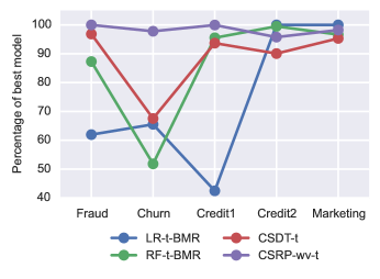
Figure 1: Comparison of the savings of the algorithms versus the highest savings in each database. The $CSRP-wt$ is very close to the best result in all the databases. Additionally, even though the $LR-BMR$ is the best algorithm in two databases, the performance in the other three is very poor.

Subsequently, in order to statistically sort the classifiers we computed the Friedman ranking (F-Rank) statistic [40]. This rank increases with the cost of the algorithms. We also calculate the average savings of each algorithm compared with the highest savings in each set (perBest), as a measure of how close are the savings of an algorithm to the best result. In TABLE VIII, the results are shown. It is observed that the first six algorithms, according to the F-Rank, belong to the $ECSDT$ family. In particular, the best three classifiers is the ensemble of cost-sensitive decision trees using the random patches approach. Giving the best result the one that blends the base classifiers using weighted voting method. Moreover as shown in TABLE IX, this method ranks on each dataset 1, 2, 2, 5 and 3, respectively. For comparison the best method from an other family is the $RF$ with $BMR$, which ranks 14, 14, 8, 2 and 9.

TABLE VIII: Savings Friedman ranking and average percentage of best result

Family	Algorithm	F-Rank	perBest
ECSDT	CSRP-wv-t	2.6	98.35
ECSDT	CSRP-s-t	3.4	97.72
ECSDT	CSRP-mv-t	4.0	94.99
ECSDT	CSB-wv-t	5.6	95.49
ECSDT	CSP-wv-t	7.4	94.72
ECSDT	CSB-mv-t	8.2	91.39
ECSDT	CSRF-wv-t	9.4	84.35
BMR	RF-t-BMR	9.4	86.16
ECSDT	CSP-s-t	9.6	93.80
ECSDT	CSP-mv-t	10.2	91.00
ECSDT	CSB-s-t	10.2	93.12
BMR	LR-t-BMR	11.2	73.98
CPS	RF-r	11.6	77.37
CST	CSDT-t	12.6	88.69
CST	CSLR-t	14.4	83.34
ECSDT	CSRF-mv-t	15.2	70.88
ECSDT	CSRF-s-t	16.0	75.68
CI	RF-u	17.2	52.83
CPS	LR-r	19.0	63.39
BMR	DT-t-BMR	19.0	60.05
CPS	LR-o	21.0	53.05
CPS	DT-r	22.6	35.33
CI	LR-u	22.8	40.43
CPS	RF-o	22.8	34.81
CI	DT-u	24.4	27.01
CPS	DT-o	25.0	24.25
CI	DT-t	26.0	16.14
CI	RF-t	26.2	16.73
CI	LR-t	28.0	1.19

(a) Comparison of the Friedman ranking.

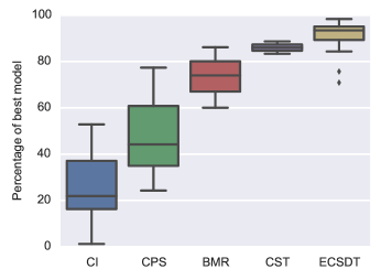
(b) Comparison of the average savings of the algorithms versus the highest savings.

Figure 2: Comparison of the results by family of classifiers. The $ECSDT$ family has the best performance measured either by Friedman ranking or average percentage of best model.

TABLE IX: Savings ranks of best algorithm of each family by database

Algorithm	Fraud	Churn	Credit1	Credit2	Marketing
RF-u	17	18	5	23	23
RF-r	20	13	3	3	19
RF-t-BMR	14	14	8	2	9
CSDT-t	10	11	16	14	12
CSRP-wv-t	1	2	2	5	3

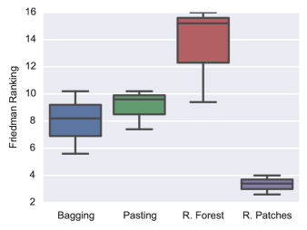
(a) Comparison by inducer methodology.

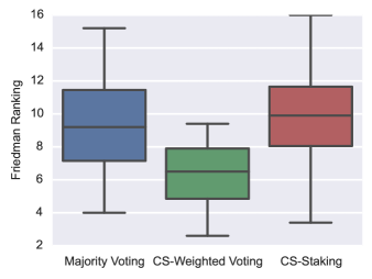
(b) Comparison by combination of base classifiers approach.

Figure 3: Comparison of the Friedman ranking within the $ECSDT$ family. Overall, the random inducer method that provides the best results is the $CSRP$. Moreover, the best combination method compared by Friedman ranking is the cost-sensitive weighted voting.

Moreover, when analyzing the perBest statistic, it is observed that it follows almost the same order as the F-Rank. Notwithstanding, there are cases in which algorithms ranks are different in the two statistics, for example the $CSDT-t$ algorithm has a lower F-Rank than the $RF-BMR$, but the perBest if better. This happens because, the F-Rank does not take into account the difference in savings within algorithms. This can be further investigated in Figure 1. Even that ranks of the $BMR$ models are better than the $CSDT$, the latter is on average closer to the best performance method in each set. Moreover, it is confirmed that the $CSRP-wt$ is very close to the best result in all cases. Lastly, it is shown why the F-Rank of the $LR-BMR$ is high, given the fact that is the best model in two databases. The reason for that, is because the performance on the other sets is very poor.

TABLE X: Results as measured by F1Score

Family	Algorithm	Fraud			Churn			Credit 1			Credit 2			Marketing
CI	DT-t	0.4458	$\pm$	0.0133	0.0733	$\pm$	0.0198	0.2593	$\pm$	0.0068	0.2614	$\pm$	0.0083	0.2647	$\pm$	0.0079
	LR-t	0.1531	$\pm$	0.0045	0.0000	$\pm$	0.0000	0.0494	$\pm$	0.0277	0.0155	$\pm$	0.0037	0.2702	$\pm$	0.0125
	RF-t	0.2061	$\pm$	0.0041	0.0249	$\pm$	0.0146	0.2668	$\pm$	0.0085	0.0887	$\pm$	0.0061	0.2884	$\pm$	0.0116
	DT-u	0.1502	$\pm$	0.0066	0.1175	$\pm$	0.0103	0.2276	$\pm$	0.0044	0.3235	$\pm$	0.0055	0.2659	$\pm$	0.0061
	LR-u	0.0241	$\pm$	0.0163	0.1222	$\pm$	0.0098	0.3160	$\pm$	0.0314	0.3890	$\pm$	0.0053	0.3440	$\pm$	0.0083
	RF-u	0.0359	$\pm$	0.0065	0.1346	$\pm$	0.0112	0.3193	$\pm$	0.0053	0.3815	$\pm$	0.0051	0.3088	$\pm$	0.0065
CPS	DT-r	0.4321	$\pm$	0.0086	0.1206	$\pm$	0.0132	0.2310	$\pm$	0.0049	0.3409	$\pm$	0.0046	0.2739	$\pm$	0.0076
	LR-r	0.1846	$\pm$	0.0123	0.1258	$\pm$	0.0111	0.3597	$\pm$	0.0156	0.3793	$\pm$	0.0049	0.3374	$\pm$	0.0101
	RF-r	0.2171	$\pm$	0.0100	0.1450	$\pm$	0.0131	0.3361	$\pm$	0.0067	0.3570	$\pm$	0.0048	0.3103	$\pm$	0.0075
	DT-o	0.4495	$\pm$	0.0063	0.1022	$\pm$	0.0180	0.2459	$\pm$	0.0081	0.3258	$\pm$	0.0056	0.2634	$\pm$	0.0089
	LR-o	0.1776	$\pm$	0.0117	0.1085	$\pm$	0.0203	0.3769	$\pm$	0.0067	0.3804	$\pm$	0.0044	0.3568	$\pm$	0.0102
	RF-o	0.2129	$\pm$	0.0080	0.0841	$\pm$	0.0201	0.3281	$\pm$	0.0078	0.3212	$\pm$	0.0054	0.3083	$\pm$	0.0093
BMR	DT-t-BMR	0.2139	$\pm$	0.0215	0.0941	$\pm$	0.0157	0.1514	$\pm$	0.0390	0.3338	$\pm$	0.0052	0.2433	$\pm$	0.0071
	LR-t-BMR	0.1384	$\pm$	0.0044	0.1370	$\pm$	0.0150	0.1915	$\pm$	0.0340	0.3572	$\pm$	0.0045	0.2954	$\pm$	0.0079
	RF-t-BMR	0.2052	$\pm$	0.0183	0.1264	$\pm$	0.0156	0.3186	$\pm$	0.0072	0.3551	$\pm$	0.0053	0.2744	$\pm$	0.0070
CST	CSLR-t	0.2031	$\pm$	0.0065	0.1134	$\pm$	0.0151	0.1454	$\pm$	0.0517	0.3363	$\pm$	0.0045	0.2339	$\pm$	0.0051
	CSDT-t	0.2522	$\pm$	0.0980	0.1288	$\pm$	0.0194	0.2754	$\pm$	0.0059	0.3483	$\pm$	0.0046	0.2680	$\pm$	0.0060
ECSDT	CSB-mv-t	0.2112	$\pm$	0.0125	0.1481	$\pm$	0.0122	0.2927	$\pm$	0.0108	0.3503	$\pm$	0.0046	0.2758	$\pm$	0.0072
	CSB-wv-t	0.2112	$\pm$	0.0091	0.1686	$\pm$	0.0125	0.2926	$\pm$	0.0108	0.3503	$\pm$	0.0046	0.2757	$\pm$	0.0072
	CSB-s-t	0.2072	$\pm$	0.0103	0.1554	$\pm$	0.0121	0.2818	$\pm$	0.0075	0.3533	$\pm$	0.0046	0.2799	$\pm$	0.0074
	CSP-mv-t	0.2098	$\pm$	0.0126	0.1480	$\pm$	0.0136	0.2903	$\pm$	0.0108	0.3499	$\pm$	0.0044	0.2749	$\pm$	0.0064
	CSP-wv-t	0.2099	$\pm$	0.0054	0.1651	$\pm$	0.0120	0.2905	$\pm$	0.0110	0.3498	$\pm$	0.0045	0.2749	$\pm$	0.0064
	CSP-s-t	0.2064	$\pm$	0.0069	0.1590	$\pm$	0.0099	0.2809	$\pm$	0.0062	0.3524	$\pm$	0.0046	0.2778	$\pm$	0.0104
	CSRF-mv-t	0.2208	$\pm$	0.0022	0.1081	$\pm$	0.0224	0.2994	$\pm$	0.0226	0.3560	$\pm$	0.0118	0.2780	$\pm$	0.0106
	CSRF-wv-t	0.2175	$\pm$	0.0019	0.1220	$\pm$	0.0234	0.2992	$\pm$	0.0236	0.3549	$\pm$	0.0069	0.2552	$\pm$	0.0187
	CSRF-s-t	0.2169	$\pm$	0.0045	0.1304	$\pm$	0.0162	0.2916	$\pm$	0.0236	0.3540	$\pm$	0.0071	0.2578	$\pm$	0.0186
	CSRP-mv-t	0.2691	$\pm$	0.0054	0.1511	$\pm$	0.0110	0.4031	$\pm$	0.0079	0.3743	$\pm$	0.0050	0.2916	$\pm$	0.0062
	CSRP-wv-t	0.2780	$\pm$	0.0041	0.1710	$\pm$	0.0140	0.4049	$\pm$	0.0066	0.3721	$\pm$	0.0051	0.2781	$\pm$	0.0063
	CSRP-s-t	0.2735	$\pm$	0.0148	0.1622	$\pm$	0.0103	0.3953	$\pm$	0.0141	0.3720	$\pm$	0.0049	0.2922	$\pm$	0.0137
(those models with the highest F1Score are market as bold)

Furthermore Figure 2a, shows the Friedman ranking of each family of classifiers. The $ECSDT$ methods are overall better, followed by the $BMR$ and the $CST$ methods. As expected, the $CI$ family is the one that performs the worst. Nevertheless, there is a significant variance within the ranks in the $ECSDT$ family, as the best one has a Friedman ranking of 2.6 and the worst 16. Similar results are found when observing the perBest shown in Figure 2b. However, in the case of the perBest, the $CST$ methods perform better than the $BMR$. It is important, in both cases it is confirmed that the $ECSDT$ family of methods is the one that arise to the best results as measured by savings.

We further investigate the different methods that compose the $ECSDT$ family, first by inducer methods and by the combination approach. In Figure 3a, the Friedman ranking of the $ECSDT$ methods grouped by inducer algorithm are shown. It is observed that the worst method is the random forest methodology. This may be related to the fact that within the random inducer methods, this is the only one that also modified the learner algorithm in the sense that it randomly select features for each step during the decision tree growing. Moreover, as expected the bagging and pasting methods perform quite similar, after all the only difference is that in bagging the sampling is done with replacement, while it is not the case in pasting. In general the best methodology is random patches. Additionally, in Figure 3b, a similar analysis is made taking into account the combination of base classifiers approach. In this case, the best combination method is weighted voting, while majority voting and staking have a similar performance.

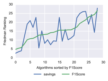
Figure 4: Comparison of the Friedman ranking of the savings and F1Score sorted by F1Score ranking. The best two algorithms according to their Friedman rank of F1Score are indeed the best ones measured by the Friedman rank of the savings. However, this relation does not consistently hold for the other algorithms as the correlation between the rankings is just 65.10%.

Finally, in TABLE X the results of the algorithms measured by F1Score are shown. It is observed that the model with the highest savings is not the same as the one with the highest F1Score in all of the databases, corroborating the conclusions from [8], as selecting a method by a traditional statistic does not give the same result as selecting it using a business oriented measure such as financial savings. This can be further examined in Figure 4, where the ranking of the F1Score and savings are compared. It is observed that the best two algorithms according to their Friedman rank of F1Score are indeed the best ones measured by the Friedman rank of the savings. However, this relation does not consistently hold for the other algorithms as the correlation between the rankings is just 65.10%.

7 Conclusions and future work

In this paper we proposed a new framework of ensembles of example-dependent cost-sensitive decision-trees by creating cost-sensitive decision trees using four different random inducer methods and then blending them using three different combination approaches. The proposed method was tested using five databases, from four real-world applications: credit card fraud detection, churn modeling, credit scoring and direct marketing. We have shown theoretically and experimentally that our method ranks the best and outperforms state-of-the-art example-dependent cost-sensitive methodologies, when measured by financial savings.

In total, our framework is composed of 12 different algorithms, since the example-dependent cost-sensitive ensemble can be constructed by inducing the base classifiers using either bagging, pasting, random forest or random patches, and then blending them using majority voting, cost-sensitive weighted voting or cost-sensitive stacking. When analyzing the results within our proposed framework, it is observed that the inducer method that performs the best is random patches algorithm. Furthermore, the random patches algorithm is the one with the lowest complexity as each base classifier is learned on a smaller subset than with the other inducer methods. Nevertheless, there is no clear winner among the different combination methods. Since the most time consuming step is inducing and constructing the base classifiers, testing all combination methods does not add a significant additional complexity.

Our results show the importance of using the real example-dependent financial costs associated with real-world applications. In particular, we found significant differences in the results when evaluating a model using a traditional cost-insensitive measure such as the accuracy or F1Score, than when using the savings. The final conclusion is that it is important to use the real practical financial costs of each context.

To improve the results, future research should be focused on developing an example-dependent cost-sensitive boosting approach. For some applications boosting methods have proved to outperform the bagging algorithms. Moreover, the methods covered in this work are all batch, in the sense that the batch algorithms keeps the system weights constant while calculating the evaluation measures. However in some applications such as fraud detection, the evolving patters due to change in the fraudsters behavior is not capture by using batch methods. Therefore, the need for investigate this problem from an online-learning perspective.

References

- [1] C. Elkan, “The Foundations of Cost-Sensitive Learning,” in Seventeenth International Joint Conference on Artificial Intelligence, 2001, pp. 973–978.
- [2] E. Ngai, Y. Hu, Y. Wong, Y. Chen, and X. Sun, “The application of data mining techniques in financial fraud detection: A classification framework and an academic review of literature,” Decision Support Systems, vol. 50, no. 3, pp. 559–569, Feb. 2011.
- [3] T. Verbraken, W. Verbeke, and B. Baesens, “A novel profit maximizing metric for measuring classification performance of customer churn prediction models,” IEEE Transactions on Knowledge and Data Engineering, vol. 25, no. 5, pp. 961–973, 2013.
- [4] B. Zadrozny, J. Langford, and N. Abe, “Cost-sensitive learning by cost-proportionate example weighting,” in Third IEEE International Conference on Data Mining. IEEE Comput. Soc, 2003, pp. 435–442.
- [5] T. Verbraken, C. Bravo, R. Weber, and B. Baesens, “Development and application of consumer credit scoring models using profit-based classification measures,” European Journal of Operational Research, vol. 238, no. 2, pp. 505–513, Oct. 2014.
- [6] C. Drummond and R. Holte, “C4.5, class imbalance, and cost sensitivity: why under-sampling beats over-sampling,” in Workshop on Learning from Imbalanced Datasets II, ICML, Washington, DC, USA, 2003.
- [7] O. M. Aodha and G. J. Brostow, “Revisiting Example Dependent Cost-Sensitive Learning with Decision Trees,” in 2013 IEEE International Conference on Computer Vision, Washington, DC, USA, Dec. 2013, pp. 193–200.
- [8] A. Correa Bahnsen, A. Stojanovic, D. Aouada, and B. Ottersten, “Cost Sensitive Credit Card Fraud Detection Using Bayes Minimum Risk,” in 2013 12th International Conference on Machine Learning and Applications. Miami, USA: IEEE, Dec. 2013, pp. 333–338.
- [9] A. Correa Bahnsen, D. Aouada, and B. Ottersten, “Example-Dependent Cost-Sensitive Logistic Regression for Credit Scoring,” in 2014 13th International Conference on Machine Learning and Applications. Detroit, USA: IEEE, 2014, pp. 263–269.
- [10] ——, “Example-Dependent Cost-Sensitive Decision Trees,” Expert Systems with Applications, vol. inpress, 2015.
- [11] G. Louppe and P. Geurts, “Ensembles on random patches,” in ECML PKDD’12 Proceedings of the 2012 European conference on Machine Learning and Knowledge Discovery in Databases. Springer Berlin Heidelberg, 2012, pp. 346–361.
- [12] L. Rokach, “Ensemble-based classifiers,” Artificial Intelligence Review, vol. 33, no. 1-2, pp. 1–39, Nov. 2009.
- [13] Z.-H. Zhou, Ensemble Methods Foundations and Algorithms. Boca Raton, FL, US: CRC Press, 2012.
- [14] L. Breiman, “Bagging predictors,” Machine Learning, vol. 24, no. 2, pp. 123–140, Aug. 1996.
- [15] ——, “Pasting small votes for classification in large databases and on-line,” Machine Learning, vol. 103, pp. 85–103, 1999.
- [16] ——, “Random Forests,” Machine Learning, vol. 45, pp. 5–32, 2001.
- [17] H. Masnadi-shirazi and N. Vasconcelos, “Cost-Sensitive Boosting,” IEEE Transactions on Pattern Analysis and Machine Intelligence, vol. 33, no. 2, pp. 294–309, 2011.
- [18] W. Street, “Bagging with Adaptive Costs,” IEEE Transactions on Knowledge and Data Engineering, vol. 20, no. 5, pp. 577–588, May 2008.
- [19] T. A. Nesbitt, “Cost-Sensitive Tree-Stacking : Learning with Variable Prediction Error Costs,” Ph.D. dissertation, University of California, Los Angeles, 2010.
- [20] S. Lomax and S. Vadera, “A survey of cost-sensitive decision tree induction algorithms,” ACM Computing Surveys, vol. 45, no. 2, pp. 1–35, Feb. 2013.
- [21] T. Hastie, R. Tibshirani, and J. Friedman, The Elements of Statistical Learning: Data Mining, Inference, and Prediction, 2nd ed. Stanford, CA: Springer, 2009.
- [22] C. Whitrow, D. J. Hand, P. Juszczak, D. J. Weston, and N. M. Adams, “Transaction aggregation as a strategy for credit card fraud detection,” Data Mining and Knowledge Discovery, vol. 18, no. 1, pp. 30–55, Jul. 2008.
- [23] T. Dietterich, “Ensemble methods in machine learning,” in Multiple classifier systems. Springer, 2000, pp. 1–15.
- [24] L. K. Hansen and P. Salamon, “Neural network ensembles,” IEEE Transactions on Pattern Analysis and Machine Intelligence, vol. 12, no. October, pp. 993–1001, 1990.
- [25] L. Lam and S. Y. Suen, “Application of majority voting to pattern recognition: an analysis of its behavior and performance,” IEEE Transactions on Systems Man and Cybernetics Part A Systems and Humans, vol. 27, no. 5, pp. 553–568, 1997.
- [26] B. Draper, C. Brodley, and P. Utgoff, “Goal-directed classification using linear machine decision trees,” IEEE Transactions on Pattern Analysis and Machine Intelligence, vol. 16, no. 9, pp. 888–893, 1994.
- [27] K. Ting, “An instance-weighting method to induce cost-sensitive trees,” IEEE Transactions on Knowledge and Data Engineering, vol. 14, no. 3, pp. 659–665, 2002.
- [28] C. X. Ling, Q. Yang, J. Wang, and S. Zhang, “Decision trees with minimal costs,” in Twenty-first international conference on Machine learning - ICML ’04, no. Icml. New York, New York, USA: ACM Press, 2004, p. 69.
- [29] J. Li, X. Li, and X. Yao, “Cost-Sensitive Classification with Genetic Programming,” in 2005 IEEE Congress on Evolutionary Computation, vol. 3. IEEE, 2005, pp. 2114–2121.
- [30] M. Kretowski and M. Grześ, “Evolutionary induction of cost-sensitive decision trees,” in Foundations of Intelligent Systems. Springer Berlin Heidelberg, 2006, pp. 121–126.
- [31] S. Vadera, “CSNL: A cost-sensitive non-linear decision tree algorithm,” ACM Transactions on Knowledge Discovery from Data, vol. 4, no. 2, pp. 1–25, 2010.
- [32] D. H. Wolpert, “Stacked generalization,” Neural Networks, vol. 5, pp. 241–259, 1992.
- [33] A. Correa Bahnsen, A. Stojanovic, D. Aouada, and B. Ottersten, “Improving Credit Card Fraud Detection with Calibrated Probabilities,” in Proceedings of the fourteenth SIAM International Conference on Data Mining, Philadelphia, USA, 2014, pp. 677 – 685.
- [34] E. Ngai, L. Xiu, and D. Chau, “Application of data mining techniques in customer relationship management: A literature review and classification,” Expert Systems with Applications, vol. 36, no. 2, pp. 2592–2602, Mar. 2009.
- [35] A. Correa Bahnsen, D. Aouada, and B. Ottersten, “A novel cost-sensitive framework for customer churn predictive modeling,” Decision Analytics, vol. inpress, 2015.
- [36] J. He, Y. Zhang, Y. Shi, S. Member, and G. Huang, “Domain-Driven Classification Based on Multiple Criteria and Multiple Constraint-Level Programming for Intelligent Credit Scoring,” IEEE Transactions on Knowledge and Data Engineering, vol. 22, no. 6, pp. 826–838, 2010.
- [37] L. C. Thomas, R. M. Oliver, and D. J. Hand, “A survey of the issues in consumer credit modelling research,” Journal of the Operational Research Society, vol. 56, no. 9, pp. 1006–1015, Jul. 2005.
- [38] S. Moro, R. Laureano, and P. Cortez, “Using data mining for bank direct marketing: An application of the crisp-dm methodology,” in European Simulation and Modelling Conference, Guimares, Portugal, 2011, pp. 117–121.
- [39] F. Pedregosa, G. Varoquaux, A. Gramfort, V. Michel, B. Thirion, O. Grisel, M. Blondel, P. Prettenhofer, R. Weiss, V. Dubourg, J. Vanderplas, A. Passos, D. Cournapeau, M. Brucher, M. Perrot, and E. Duchesnay, “Scikit-learn: Machine learning in Python,” Journal of Machine Learning Research, vol. 12, pp. 2825–2830, 2011.
- [40] J. Demšar, “Statistical Comparisons of Classifiers over Multiple Data Sets,” Journal of Machine Learning Research, vol. 7, pp. 1–30, 2006.