Simple regret for infinitely many armed bandits

Abstract

We consider a stochastic bandit problem with infinitely many arms. In this setting, the learner has no chance of trying all the arms even once and has to dedicate its limited number of samples only to a certain number of arms. All previous algorithms for this setting were designed for minimizing the cumulative regret of the learner. In this paper, we propose an algorithm aiming at minimizing the simple regret. As in the cumulative regret setting of infinitely many armed bandits, the rate of the simple regret will depend on a parameter $\beta$ characterizing the distribution of the near-optimal arms. We prove that depending on $\beta$, our algorithm is minimax optimal either up to a multiplicative constant or up to a $\log(n)$ factor. We also provide extensions to several important cases: when $\beta$ is unknown, in a natural setting where the near-optimal arms have a small variance, and in the case of unknown time horizon.

1 Introduction

Sequential decision making has been recently fueled by several industrial applications, e.g., advertisement, and recommendation systems. In many of these situations, the learner is faced with a large number of possible actions, among which it has to make a decision. The setting we consider is a direct extension of a classical decision-making setting, in which we only receive feedback for the actions we choose, the bandit setting. In this setting, at each time $t$, the learner can choose among all the actions (called the arms) and receives a sample (reward) from the chosen action, which is typically a noisy characterization of the action. The learner performs $n$ such rounds and its performance is then evaluated with respect to some criterion, for instance the cumulative regret or the simple regret.

In the classical, multi-armed bandit setting, the number of actions is assumed to be finite and small when compared to the number of decisions. In this paper, we consider an extension of this setting to infinitely many actions, the infinitely many armed bandits (Berry et al., 1997; Wang et al., 2008; Bonald & Proutière, 2013). Inevitably, the sheer amount of possible actions makes it impossible to try each of them even once. Such a setting is practically relevant for cases where one faces a finite, but extremely large number of actions. This setting was first formalized by Berry et al. (1997) as follows. At each time $t$, the learner can either sample an arm (a distribution) that has been already observed in the past, or sample a new arm, whose mean $\mu$ is sampled from the mean reservoir distribution $\mathcal{L}$.

The additional challenges of the infinitely many armed bandits with respect to the multi-armed bandits come from two sources. First, we need to find a good arm among the sampled ones. Second, we need to sample (at least once) enough arms in order to have (at least once) a reasonably good one. These two difficulties ask for a while which we call the arm selection tradeoff. It is different from the known exploration/exploitation tradeoff and more linked to model selection principles: On one hand, we want to sample only from a small subsample of arms so that we can decide, with enough accuracy, which one is the best one among them. On the other hand, we want to sample as many arms as possible in order to have a higher chance to sample a good arm at least once. This tradeoff makes the problem of infinitely many armed bandits significantly different from the classical bandit problem.

Berry et al. (1997) provide asymptotic, minimax-optimal (up to a $\log n$ factor) bounds for the average cumulative regret, defined as the difference between $n$ times the highest possible value $\bar{\mu}^{*}$ of the mean reservoir distribution and the mean of the sum of all samples that the learner collects. A follow-up on this result was the work of Wang et al. (2008), providing algorithms with finite-time regret bounds and the work of Bonald & Proutière (2013), giving an algorithm that is optimal with exact constants in a strictly more specific setting. In all of this prior work, the authors show that it is the shape of the arm reservoir distribution what characterizes the minimax-optimal rate of the average cumulative regret. Specifically, Berry et al. (1997) and Wang et al. (2008) assume that the mean reservoir distribution is such that, for a small $\varepsilon>0$, locally around the best arm $\bar{\mu}^{*}$, we have that

$$\mathbb{P}_{\mu\sim\mathcal{L}}\left(\bar{\mu}^{*}-\mu\geq\varepsilon\right)\approx\varepsilon^{\beta},$$ (1)

that is, they assume that the mean reservoir distribution is $\beta$-regularly varying in $\bar{\mu}^{*}$. When this assumption is satisfied with a known $\beta$, their algorithms achieve an expected cumulative regret of order

$$\!\!\!\!\!\mathbb{E}\left[R_{n}\right]\!=\!\mathcal{O}\left(\max\left(n^{\frac{\beta}{\beta+1}}\operatorname{polylog}n,\sqrt{n}\operatorname{polylog}n\right)\right).$$ (2)

The limiting factor in the general setting is a $1/\sqrt{n}$ rate for estimating the mean of any of the arms with $n$ samples. This gives the rate (2) of $\sqrt{n}$. It can be refined if the distributions of the arms, that are sampled from the mean reservoir distribution, are Bernoulli of mean $\mu$ and $\bar{\mu}^{*}=1$ or in the same spirit, if the distributions of the arms are defined on $[0,1]$ and $\bar{\mu}^{*}=1$ as

$$\mathbb{E}\left[R_{n}\right]=\mathcal{O}\left(n^{\frac{\beta}{\beta+1}}\operatorname{polylog}n\right).$$ (3)

Bonald & Proutière (2013) refine the result (3) even more by removing the $\operatorname{polylog}n$ factor and proving upper and lower bounds that exactly match, even in terms of constants, for a specific sub-case of a uniform mean reservoir distribution. Notice that the rate (3) is faster than the more general rate (2). This comes from the fact that they assume that the variances of the arms decay with their quality, making finding a good arm easier. For both rates (2 and 3), $\beta$ is the key parameter for solving the arm selection tradeoff: with smaller $\beta$ it is more likely that the mean reservoir distribution outputs a high value, and therefore, we need fewer arms for the optimal arm selection tradeoff.

Previous algorithms for this setting were designed for minimizing the cumulative regret of the learner which optimizes the cumulative sum of the rewards. In this paper, we consider the problem of minimizing the simple regret. We want to select an optimal arm given the time horizon $n$. The simple regret is the difference between the mean of the arm that the learner selects at time $n$ and the highest possible mean $\bar{\mu}^{*}$. The problem of minimizing the simple regret in a multi-armed bandit setting (with finitely many arms) has recently attracted significant attention (Even-Dar et al., 2006; Audibert et al., 2010; Kalyanakrishnan et al., 2012; Kaufmann & Kalyanakrishnan, 2013; Karnin et al., 2013; Gabillon et al., 2012; Jamieson et al., 2014) and algorithms have been developed either in the setting of a fixed budget which aims at finding an optimal arm or in the setting of a floating budget which aims at finding an $\varepsilon$-optimal arm.

All prior work on simple regret considers a fixed number of arms that will be ultimately all explored and cannot be applied to an infinitely many armed bandits or to a bandit problem with the number of arms larger than the available time budget. An example where efficient strategies for minimizing the simple regret of an infinitely many armed bandit are relevant is the search of a good biomarker in biology, a single feature that performs best on average (Hauskrecht et al., 2006). There can be too many possibilities that we cannot afford to even try each of them in a reasonable time. Our setting is then relevant for this special case of single feature selection. In this paper, we provide the following results for the simple regret of an infinitely many armed bandit, a problem that was not considered before.

• We propose an algorithm that for a fixed horizon $n$ achieves the finite-time simple regret rate

  $$r_{n}=\mathcal{O}\left(\max\left(n^{-1/2},n^{-\frac{1}{\beta}}\operatorname{polylog}n\right)\right).$$

• We prove corresponding lower bounds for this infinitely many armed simple regret problem, that are matching up to a multiplicative constant for $\beta<2$, and matching up to a $\operatorname{polylog}n$ for $\beta\geq 2$.

• We provide three important extensions:

  • The first extension concerns the case where the distributions of the arms are defined on $[0,1]$ and where $\bar{\mu}^{*}=1$. In this case, replacing the Hoeffding bound in the confidence term of our algorithm by a Bernstein bound, bounds the simple regret as

    $$r_{n}\!=\!\mathcal{O}\big{(}\!\max(\tfrac{1}{n}\operatorname{polylog}n,(n\log n)^{-\frac{1}{\beta}}\operatorname{polyloglog}n\big{)}.$$

  • The second extension treats unknown $\beta$. We prove that it is possible to estimate $\beta$ with enough precision, so that its knowledge is not necessary for implementing the algorithm. This can be also applied to the prior work (Berry et al., 1997; Wang et al., 2008) where $\beta$ is also necessary for implementation and optimal bounds.

  • Finally, in the third extension we make the algorithm anytime using known tools.

• We provide simple numerical simulations of our algorithm and compare it to infinitely many armed bandit algorithms optimizing cumulative regret and to multi-armed bandit algorithms optimizing simple regret.

Besides research on infinitely many arms bandits, there exist many other settings where the number of actions may be infinite. One class of examples is fixed design such as linear bandits (Dani et al., 2008) other settings consider bandits in known or unknown metric space (Kleinberg et al., 2008; Munos, 2014; Azar et al., 2014). These settings assume regularity properties that are very different from the properties assumed in the infinitely many arm bandits and give rise to significantly different approaches and results. Furthermore, in classic optimization settings, one assumes that in addition to the rewards, there is side information available through the position of the arms, combined with a smoothness assumption on the reward, which is much more restrictive. On the contrary, we only assume a bound on the proportion of near-optimal arms. It is not always the case that there is side information through a topology on the arms. In such cases, the infinitely many armed setting is applicable while optimization routines are not.

2 Setting

Learning setting

Let $\tilde{\mathcal{L}}$ be a distribution of distributions. We call $\tilde{\mathcal{L}}$ the arm reservoir distribution, i.e., the distribution of the means of arms. Let $\mathcal{L}$ be the distribution of the means of the distributions output by $\tilde{\mathcal{L}}$, i.e., the mean reservoir distribution. Let $\mathbb{A}_{t}$ denote the changing set of $K_{t}$ arms at time $t$.

At each time $t+1$, the learner can either choose an arm $k_{t+1}$ among the set of the $K_{t}$ arms $\mathbb{A}_{t}=\{\nu_{1},\ldots,\nu_{K_{t}}\}$ that it has already observed (in this case, $K_{t+1}=K_{t}$ and $\mathbb{A}_{t+1}=\mathbb{A}_{t}$), or choose to get a sample of a new arm that is generated according to $\tilde{\mathcal{L}}$ (in this case, $K_{t+1}=K_{t}+1$ and $\mathbb{A}_{t+1}=\mathbb{A}_{t}\cup\{\nu_{K_{t}+1}\}$ where $\nu_{K_{t}+1}\sim\tilde{\mathcal{L}}$). Let $\mu_{i}$ be the mean of arm $i$, i.e., the mean of distribution $\nu_{i}$ for $i\leq K_{t}$. We assume that $\mu_{i}$ always exists.

In this setting, the learner observes a sample at each time. At the end of the horizon, which happens at a given time $n$, the learner has to output an arm $\widehat{k}\leq K_{n}$, and its performance is assessed by the simple regret

$$r_{n}=\bar{\mu}^{*}-\mu_{\widehat{k}},$$

where $\bar{\mu}^{*}=\operatorname*{arg\,inf}_{m}\left(\mathbb{P}_{\mu\sim\mathcal{L}}(\mu\leq m)=1\right)$ is the right end point of the domain.

Assumption on the samples

The domain of the arm reservoir distribution $\tilde{\mathcal{L}}$ are distributions of arm samples. We assume that these distributions $\nu$ are bounded.

Assumption 1 (Bounded distributions in the domain of $\tilde{\mathcal{L}}$).

Let $\nu$ be a distribution in the domain of $\tilde{\mathcal{L}}$. Then $\nu$ is a bounded distribution. Specifically, there exists an universal constant $C>0$ such that the domain of $\nu$ is contained in $[-C,C]$.

This implies that the expectations of all distributions generated by $\tilde{\mathcal{L}}$ exist, are finite, and bounded by $C$. In particular, this implies that

$$\bar{\mu}^{*}=\operatorname*{arg\,inf}_{m}\left(\mathbb{P}_{\mu\sim\mathcal{L}}(\mu\leq m)=1\right)<+\infty,$$

which implies that the regret is well defined, and that the domain of $\mathcal{L}$ is bounded by $2C$. Note that all the results that we prove hold also for sub-Gaussian distributions $\nu$ and bounded $\mathcal{L}$. Furthermore, it would possible to relax the sub-Gaussianity using different estimators recently developed for heavy-tailed distributions (Catoni, 2012).

Assumption on the arm reservoir distribution

We now assume that the mean reservoir distribution $\mathcal{L}$ has a certain regularity in its right end point, which is a standard assumption for infinitely many armed bandits. Note that this implies that the distribution of the means of the arms is in the domain of attraction of a Weibull distribution, and that it is related to assuming that the distribution is $\beta$ regularly varying in its end point $\bar{\mu}^{*}$.

Assumption 2 ($\beta$ regularity in $\bar{\mu}^{*}$).

Let $\beta>0$. There exist $\tilde{E},\tilde{E}^{\prime}>0$, and $0<\tilde{B}<1$ such that for any $0\leq\varepsilon\leq\tilde{B}$,

$$\tilde{E}^{\prime}\varepsilon^{\beta}\geq\mathbb{P}_{\mu\sim\mathcal{L}}\left(\mu>\bar{\mu}^{*}-\varepsilon\right)\geq\tilde{E}\varepsilon^{\beta}.$$

This assumption is the same as the classical one (1). Standard bounded distributions satisfy Assumption 2 for a specific $\beta$, e.g., all the $\beta$ distributions, in particular the uniform distribution, etc.

3 Main results

In this section, we first present the information theoretic lower bounds for the infinitely many armed bandits with simple regret as the objective. We then present our algorithm and its analysis proving the upper bounds that match the lower bounds — in some cases, depending on $\beta$, up to a $\operatorname{polylog}n$ factor. This makes our algorithm (almost) minimax optimal. Finally, we provide three important extensions as corollaries.

3.1 Lower bounds

The following theorem exhibits the information theoretic complexity of our problem and is proved in Appendix C. Note that the rates crucially depend on $\beta$.

Theorem 1 (Lower bounds).

Let us write $\mathcal{S}_{\beta}$ for the set of distributions of arms distributions $\tilde{\mathcal{L}}$ that satisfy Assumptions 1 and 2 for the parameters $\beta,\tilde{E},\tilde{E}^{\prime},C$. Assume that $n$ is larger than a constant that depends on $\beta,\tilde{E},\tilde{E}^{\prime},\tilde{B},C$. Depending on the value of $\beta$, we have the following results, for any algorithm $\mathcal{A}$, where $v$ is a small enough constant.

• Case $\beta<2$: With probability larger than $1/3$,

  $$\inf_{\mathcal{A}}\sup_{\tilde{\mathcal{L}}\in\mathcal{S}_{\beta}}r_{n} \geq vn^{-1/2}.$$

• Case $\beta\geq 2$: With probability larger than $1/3$,

  $$\inf_{\mathcal{A}}\sup_{\tilde{\mathcal{L}}\in\mathcal{S}_{\beta}}r_{n}\geq vn^{-1/\beta}.$$

Remark 1.

Comparing these results with the rates for the cumulative regret problem (2) from the prior work, one can notice that there are two regimes for the cumulative regret results. One regime is characterized by a rate of $\sqrt{n}$ for $\beta\leq 1$, and the other characterized by a $n^{\beta/(1+\beta)}$ rate for $\beta\geq 1$. Both of these regimes are related to the arm selection tradeoff. The first regime corresponds to easy problems where the mean reservoir distribution puts a high mass close to $\bar{\mu}^{*}$, which favors sampling a good arm with high mean from the reservoir. In this regime, the $\sqrt{n}$ rate comes from the parametric $1/\sqrt{n}$ rate for estimating the mean of any arm with $n$ samples. The second regime corresponds to more difficult problems where the reservoir is unlikely to output a distribution with mean close to $\bar{\mu}^{*}$ and where one has to sample many arms from the reservoir. In this case, the $\sqrt{n}$ rate is not reachable anymore because there are too many arms to choose from sub-samples of arms containing good arms. The same dynamics exists also for the simple regret, where there are again two regimes, one characterized by a $n^{-1/2}$ rate for $\beta\leq 2$, and the other characterized by a $n^{-1/\beta}$ rate for $\beta\geq 2$. Provided that these bounds are tight (which is the case, up to a $\operatorname{polylog}n$, Section 3.2), one can see that there is an interesting difference between the cumulative regret problem and the simple regret one. Indeed, the change of regime is here for $\beta=2$ and not for $\beta=1$, i.e., the parametric rate of $n^{-1/2}$ is valid for larger values of $\beta$ for the simple regret. This comes from the fact that for the simple regret objective, there is no exploitation phase and everything is about exploring. Therefore, an optimal strategy can spend more time exploring the set of arms and reach the parametric rate also in situations where the cumulative regret does not correspond to the parametric rate. This has also practical implications examined empirically in Section 5.

3.2 SiRI and its upper bounds

In this section, we present our algorithm, the Simple Regret for Infinitely many arms (SiRI) and its analysis.

The SiRI algorithm

Let $b=\min(\beta,2),$ and let

$$\bar{T}_{\beta}=\lceil A(n)n^{b/2}\rceil,$$

where

$$A(n)=\begin{cases}A,&\text{if $\beta<2$}\\ A/\log(n)^{2},&\text{if $\beta=2$}\\ A/\log(n),&\text{if $\beta>2$}\end{cases}$$

where $A$ is a small constant whose precise value will depend on our analysis. Let $\log_{2}$ be the logarithm in base 2. Let us define

$$\bar{t}_{\beta}=\lfloor\log_{2}(\bar{T}_{\beta})\rfloor.$$

Let $T_{k,t}$ be the number of pulls of arm $k\leq K_{t}$, and $X_{k,u}$ for the $u$-th sample of $\nu_{k}$. The empirical mean of the samples of arm $k$ is defined as

$$\widehat{\mu}_{k,t}=\frac{1}{T_{k,t}}\sum_{u=1}^{T_{k,t}}X_{k,u}.$$

With this notation, we provide SiRI as Algorithm 1.

  Parameters: $\beta,C,\delta$

  Initial pull of arms from the reservoir:

  Choose $\bar{T}_{\beta}$ arms from the reservoir $\tilde{\mathcal{L}}$ .

  Pull each of $\bar{T}_{\beta}$ arms once.

  $t\leftarrow\bar{T}_{\beta}$

  Choice between these arms:

  while $t\leq n$ do

     For any $k\leq\bar{T}_{\beta}$:

$$B_{k,t}\leftarrow\widehat{\mu}_{k,t} +2\sqrt{\frac{C}{T_{k,t}}\log\big{(}2^{2\bar{t}_{\beta}/b}/(T_{k,t}\delta)\big{)}}$$

$$+\frac{2C}{T_{k,t}}\log\left(2^{2\bar{t}_{\beta}/b}/(T_{k,t}\delta)\right)$$ (4)

     Pull $T_{k,t}$ times the arm $k_{t}$ that maximizes $B_{k,t}$ and  receive $T_{k,t}$ samples from it.

     $t\leftarrow t+T_{k,t}$

  end while

  Output: Return the most pulled arm $\widehat{k}$.

Algorithm 1 SiRI
      Simple Regret for Infinitely Many Armed Bandits

Discussion

SiRI is a UCB-based algorithm, where the leading confidence term is of order

$$\sqrt{\frac{\log\left(n/(\delta T_{k,t})\right)}{T_{k,t}}}\cdot$$

Similar to the MOSS algorithm (Audibert & Bubeck, 2009), we divide the $\log(\cdot)$ term by $T_{k,t}$, in order to avoid additional logarithmic factors in the bound. But a simpler algorithm with a confidence term as in a classic UCB algorithm for cumulative regret,

$$\sqrt{\frac{\log(n/\delta)}{T_{k,t}}}\text{,}$$

would provide almost optimal regret, up to a $\log n$, i.e., with a slightly worse regret than what we get. It is quite interesting that with such a confidence term, SiRI is optimal for minimizing the simple regret for infinitely many armed bandits, since MOSS, as well as the classic UCB algorithm, targets the cumulative regret. The main difference between our strategy and the cumulative strategies (Berry et al., 1997; Wang et al., 2008; Bonald & Proutière, 2013) is in the number of arms sampled from the arm reservoir: For the simple regret, we need to sample more arms. Although the algorithms are related, their analyses are quite different: Our proof is event-based whereas the proof for the cumulative regret targets directly the expectations.

It is also interesting to compare SiRI with existing algorithms targeting the simple regret for finitely many arms, as the ones by Audibert et al. (2010). SiRI can be related to their UCB-E with a specific confidence term and a specific choice of the number of arms selected. Consequently, the two algorithms are related but the regret bounds obtained for UCB-E are not informative when there are infinitely many arms. Indeed, the theoretical performance of UCB-E is decreasing with the sum of the inverse of the gaps squared, which is infinite when there are infinitely many arms. In order to obtain a useful bound in this case, we need to consider a more refined analysis which is the one that leads to Theorem 2.

Remark 2.

Note that SiRI pulls series of samples from the same arm without updating the estimate which may seem wasteful. In fact, it is possible to update the estimates after each pull. On the other hand, SiRI is already minimax optimal, so one can only hope to get improvement in constants. Therefore, we present this version of SiRI, since its analysis is easier to follow.

Main result

We now state the main result which characterizes SiRI’s simple regret according to $\beta$.

Theorem 2 (Upper bounds).

Let $\delta>0$. Assume all Assumptions 1 and 2 of the model and that $n$ is larger than a large constant that depends on $\beta,\tilde{E},\tilde{E}^{\prime},\tilde{B},C$. Depending on the value of $\beta$, we have the following results, where $E$ is a large enough constant.

• Case $\beta<2$: With probability larger than $1-\delta$,

  $$r_{n} \leq En^{-1/2}\log(1/\delta)(\log(\log(1/\delta)))^{96}\sim n^{-1/2}.$$

• Case $\beta>2$: With probability larger than $1-\delta$,

  $$r_{n} \leq E(n\log(n))^{-1/\beta}(\log(\log(\log(n)/\delta)))^{96}\times$$

  $$\times\log(\log(n)/\delta)\sim(n\log n)^{-1/\beta}\operatorname{polyloglog}n.$$

• Case $\beta=2$: With probability larger than $1-\delta$,

  $$r_{n} \leq E\log(n)n^{-1/2}(\log(\log(\log(n)/\delta)))^{96}\times$$

  $$\times\log(\log(n)/\delta)\sim n^{-1/2}\log n\operatorname{polyloglog}n.$$

Short proof sketch.

In order to prove the results, the main tools are events $\xi_{1}$ and $\xi_{2}$ (Appendix B). One event controls the number of arms at a given distance from $\bar{\mu}^{*}$ and the other one controls the distance between the empirical means and the true means of the arms.

Provided that events $\xi_{1}$ and $\xi_{2}$ hold, which they do with high probability, we know that there are less than approximately $N_{u}=\bar{T}_{\beta}2^{-u}$ arms at a distance larger than $2^{-u/\beta}$ from $\bar{\mu}^{*}$, and that each arm that is at a distance larger than $2^{-u/\beta}$ from $\bar{\mu}^{*}$ will be pulled less than $P_{u}=2^{2u/\beta}$ times. After these many pulls, the algorithm recognizes that it is suboptimal.

Since a simple computation yields

$$\sum_{0\leq u\leq\log_{2}(\bar{T}_{\beta})}N_{u}P_{u}\leq\frac{n}{C},$$

we know that all the suboptimal arms at a distance further than $2^{-\log_{2}(\bar{T}_{\beta})/\beta}$ from the optimal arm are discarded since they are all sampled enough to be proved suboptimal. We thus know that an arm at a distance less than $2^{-\log_{2}(T_{\bar{\beta}})/\beta}$ from the optimal arm is selected in high probability, which concludes the proof.

The full proof(Appendix B) is quite technical, since it uses a peeling argument to correctly define the high probability event to avoid a suboptimal rate, in particular in terms of $\log n$ terms for $\beta<2$, and since we need to control accurately the number of arms at a given distance from $\bar{\mu}^{*}$ at the same time as their empirical means. ∎

Discussion

The bound we obtain is minimax optimal for $\beta<2$ without additional $\log n$ factors. We emphasize it since the previous results on infinitely many armed bandits give results which are optimal up to a $\operatorname{polylog}n$ factor for the cumulative regret, except the one by Bonald & Proutière (2013) which considers a very specific and fully parametric setting. For $\beta\geq 2$, our result is optimal up to a $\operatorname{polylog}n$ factor. We conjecture that the lower bound of Theorem 1 for $\beta\geq 2$ can be improved to $(\log(n)/n)^{1/\beta}$ and that SiRI is actually optimal up to a $\operatorname{polyloglog}(n)$ factor for $\beta>2$.

4 Extensions of SiRI

We now discuss briefly three extensions of the SiRI algorithm that are very relevant either for practical or computational reasons, or for a comparison with the prior results. In particular, we consider the cases 1) when $\beta$ is unknown, 2) in a natural setting where the near-optimal arms have a small variance, and 3) in the case of unknown time horizon. These extensions are all in some sense following from our results and from the existing literature, and we will therefore state them as corollaries.

4.1 Case of distributions on $[0,1]$ with $\bar{\mu}^{*}=1$

The first extension concerns the specific setting, particularly highlighted by Bonald & Proutière (2013) but also presented by Berry et al. (1997) and Wang et al. (2008), where the domain of the distributions of the arms are included in $[0,1]$ and where $\bar{\mu}^{*}=1$. In this case, the information theoretic complexity of the problem is smaller than the one of the general problem stated in Theorem 1. Specifically, the variance of the near-optimal arms is very small, i.e., in the order of $\varepsilon$ for an $\varepsilon$-optimal arm. This implies a better bound, in particular, that the parametric limitation of $1/\sqrt{n}$ can be circumvented. In order to prove it, the simplest way is to modify SiRI into Bernstein-SiRI, displayed in Algorithm 2. It is an Empirical Bernstein-modified SiRI algorithm that accommodates the situation of distributions of support included in $[0,1]$ with $\bar{\mu}^{*}=1$. Note that in the general case, it would provide similar results as what is provided in Theorem 2.

  Parameters: $C,\beta,\delta$

  Newly defined quantities:

  Set the number of arms as

$$\bar{T}_{\beta}=\lceil\min(n/\log(n),A(n)n^{\beta/2})\rceil,$$

  Modify the SiRI algorithm’s UCB (4) with

$$B_{k,t} \leftarrow\widehat{\mu}_{k,t}+2\widehat{\sigma}_{k,t}\sqrt{\frac{C}{T_{k,t}}\log\big{(}2^{2\bar{t}_{\beta}/b}/(T_{k,t}\delta)\big{)}}$$

$$+\frac{4C}{T_{k,t}}\log\left(2^{2\bar{t}_{\beta}/b}/(T_{k,t}\delta)\right),$$

where $\widehat{\sigma}_{k,t}^{2}$ is the empirical variance, defined as

$$\widehat{\sigma}_{k,t}^{2}=\frac{1}{T_{k,t}}\sum_{l=1}^{T_{k,t}}\left(X_{k,t}-\widehat{\mu}_{k,t}\right)^{2}.$$

  Call SiRI:

  Run SiRI on the samples using these new parameters

Algorithm 2 Bernstein-SiRI

A similar idea was already introduced by Wang et al. (2008) in the infinitely many armed setting for cumulative regret. The idea is that the confidence term is more refined using the empirical variance and hence it will be very large for a near-optimal arm, thereby enhancing exploration. Plugging this term in the proof, conditioning on the event of high probability, such that $\widehat{\sigma}_{k,t}^{2}$ is close to the true variance, and using similar ideas as Wang et al. (2008), we can immediately deduce the following corollary.

Corollary 1.

Let $\delta>0$. Assume Assumptions 1 and 2 of the model and that $n$ is larger than a large constant that depends on $\beta,\tilde{E},\tilde{E}^{\prime},\tilde{B},C$. Furthermore, assume that all the arms have distributions of support included in $[0,1]$ and that $\bar{\mu}^{*}=1$. Depending on $\beta$, we have the following results for Bernstein-SiRI.

• Case $\beta\leq 1$: The order of the simple regret is with high probability

  $$r_{n}=\mathcal{O}\left(\tfrac{1}{n}\operatorname{polylog}n\right).$$

• Case $\beta>1$: The order of the simple regret is with high probability

  $$r_{n}=\mathcal{O}\left(\left(\tfrac{1}{n}\right)^{1/\beta}\operatorname{polylog}n\right).$$

  Moreover, the rate

  $$\max\left(\frac{1}{n},\left(\tfrac{\log n}{n}\right)^{1/\beta}\right),$$

  is minimax-optimal for this problem, i.e., there exists no algorithm that achieves a better simple regret in a minimax sense.

The proof follows immediately from the proof of Theorem 2 using the empirical Bernstein bound as by Wang et al. (2008). Moreover, the lower bounds’ rates follow directly from the two facts: 1) $1/n$ is clearly a lower bound, and therefore optimal for $\beta<1$, since it takes at least $n$ samples of a Bernoulli arm that is constant times $1/n$ suboptimal, in order to discover that it is not optimal, and 2) $n^{-1/\beta}$ can be trivially deduced from Theorem 1. Bernstein-SiRI is thus minimax optimal for $\beta\geq 1$ up to a $\operatorname{polylog}n$ factor.

Discussion

Corollary 1 improves the results of Theorem 2 when $\beta\in(0,2)$. For these $\beta$, it is possible to beat the parametric rate of $1/\sqrt{n}$, since in this case, the variance of the arms decays with the quality of the arms. In this situation, for $\beta<2$, it is possible to beat the parametric rate $1/\sqrt{n}$ and keep the rate of $n^{-1/\beta}$ until $\beta\leq 1$, where the limiting rate of $1/n$ imposes its limitations: the regret cannot be smaller than the second order parametric rate of $1/n$. Here, the change point of regime is $\beta=1$ which differs from the general simple regret case but is the same as the general case of cumulative regret as discussed in Remark 1. Notice that this comes from the fact that the limiting rate is now $1/n$ and not for same reasons as for the cumulative regret.

4.2 Dealing with unknown $\beta$

In practice, the parameter $\beta$ is almost never available. Yet its knowledge is crucial for the implementation of SiRI, as well as for all the cumulative regret strategies described in (Berry et al., 1997; Wang et al., 2008; Bonald & Proutière, 2013). Consequently, a very important question is whether it is possible to estimate it well enough to obtain good results, which we answer in the affirmative.

An interesting remark is that Assumption 2 is actually related to assuming that the distribution function $\mathcal{L}$ is $\beta$ regularly varying in $\bar{\mu}^{*}$. Therefore, $\beta$ is the tail index of the distribution function of $\mathcal{L}$ and can be estimated with tools from extreme value theory (de Haan & Ferreira, 2006). Many estimators exist for estimating this tail index $\beta$, for instance, the popular Hill’s estimate (Hill, 1975), but also Pickand’s’ estimate (Pickands, 1975) and others.

However, our situation is slightly different from the one where the convergence of these estimators is proved, as the means of the arms are not directly observed. As a result, we propose another estimate, related to the estimate of Carpentier & Kim (2014), which accommodates our setting. Assume that we have observed $N$ arms, and that all of these arms have been sampled $N$ times. Let us write $\widehat{m}_{k}$ for the empirical mean estimates of the mean $m_{k}$ of these $N$ arms and define

$$\widehat{m}^{*}=\max_{k}\widehat{m}_{k}.$$

We further define

$$\widehat{p}=\frac{1}{N}\sum_{k=1}^{N}\mathbf{1}\{\widehat{m}^{*}-\widehat{m}_{k}\leq N^{-\varepsilon}\}$$

and set

$$\widehat{\beta}=-\frac{\log\widehat{p}}{\varepsilon\log N}\cdot$$ (5)

This estimate satisfies the following weak concentration inequality and its proof is in Appendix D.

Lemma 1.

Let $\underline{\beta}$ be a lower bound on $\beta$. If Assumptions 1 and 2 are satisfied and $\varepsilon<\min(\underline{\beta},1/2,1/(\underline{\beta}))$, then with probability larger than $1-\delta$, for $N$ larger than a constant that depends only on $\tilde{B}$ of Assumption 2,

$$|\widehat{\beta}-\beta| \leq\frac{\frac{\delta^{-1/\underline{\beta}}}{\underline{\beta}}+\sqrt{\log(\frac{1}{\delta})}+\max(1,\log(\tilde{E}^{\prime}),|\log(\tilde{E})|)}{\varepsilon\log N}$$

$$\leq\frac{c^{\prime}\max(\sqrt{\log(1/\delta)},\delta^{-1/\underline{\beta}})}{\varepsilon\log N},$$

where $c^{\prime}>0$ is a constant that depends only on $\varepsilon$ and the parameter $C$ of Assumption 1.

  Parameters: $C,\delta,\underline{\beta}$

  Initial phase for estimating $\beta$:

  Let $N\leftarrow n^{1/4}$ and $\varepsilon\leftarrow 1/\log\log\log(n)$.

  Sample $N$ arms from the arm reservoir $N$ times

  Compute $\widehat{\beta}$ following (5)

  Set

$$\bar{\beta}\leftarrow\widehat{\beta}+\frac{c^{\prime}\max\left(\sqrt{\log(1/\delta)},\delta^{-1/\underline{\beta}}\right)\operatorname{logloglog}n}{\log n}$$ (6)

  Call SiRI:

  Run SiRI using $\bar{\beta}$ instead of $\beta$ with $n-N^{2}=n-\sqrt{n}$ remaining samples.

Algorithm 3 $\bar{\beta}$-SiRI: $\bar{\beta}$-modified SiRI for unknown $\beta$

Let us now modify SiRI in the way as in Algorithm 3. The knowledge of $\beta$ is not anymore required, and one just needs a lower bound $\underline{\beta}$ on $\beta$. We get $\bar{\beta}$-SiRI which satisfies the following corollary.

Corollary 2.

Let the Assumptions 1 and 2 be satisfied. If $n$ is large enough with respect to a constant that depends on $\beta,\tilde{E},\tilde{E}^{\prime},\tilde{B},C$, then $\bar{\beta}-$SiRI satisfies the following:

• Case $\beta<2$: The order of the simple regret is with high probability

  $$r_{n}=\mathcal{O}\left(\tfrac{1}{\sqrt{n}}\operatorname{polyloglog}n\right).$$

• Case $\beta>2$: The order of the simple regret is with high probability

  $$r_{n}=\mathcal{O}\left(\left(\tfrac{\log n}{n}\right)^{1/\beta}\operatorname{polyloglog}n\right).$$

• Case $\beta=2$: The order of the simple regret is with high probability

  $$r_{n}=\mathcal{O}\left(\tfrac{\log n}{\sqrt{n}}\operatorname{polyloglog}n\right).$$

The proof can be deduced easily from Theorem 2 using the result from Lemma 1, noting that a $1/\log n$ rate in learning $\beta$ is fast enough to guarantee that all bounds will only be modified by a constant factor when we use $\widehat{\beta}$ instead of $\beta$ in the exponent.

Discussion

Corollary 2 implies that even in situations with unknown $\beta$, it is possible to estimate it accurately enough so that the modified $\bar{\beta}$-SiRI remains minimax-optimal up to a $\operatorname{polylog}n$, by only using a lower bound $\underline{\beta}$ on $\beta$. This is the same that holds for SiRI with known $\beta$. We would like to emphasize that $\bar{\beta}$ estimate (6) of $\beta$ can be used to improve cumulative regret algorithms that need $\beta$, such as the ones by Berry et al. (1997) and Wang et al. (2008). Similarly for these algorithms, one should spend a preliminary phase of $N^{2}=\sqrt{n}$ rounds to estimate $\beta$ and then run the algorithm of choice. This will modify the cumulative regret rates in the general setting by only a $\operatorname{polyloglog}n$ factor, which suggests that our $\beta$ estimation can be useful beyond the scope of this paper. For instance, consider the cumulative regret rate of UCB-F by Wang et al. (2008). If UCB-F uses our estimate of $\beta$ instead of the true $\beta$, it would still satisfy

$$\mathbb{E}\left[R_{n}\right]=\mathcal{O}\left(\max\left(n^{\frac{\beta}{\beta+1}}\operatorname{polylog}n,\sqrt{n}\operatorname{polylog}n\right)\right).$$

Finally, this modification can be used to prove that this problem is learnable over all mean reservoir distributions with $\beta>0$: This can be seen by setting the lower bound on $\beta$ as $\underline{\beta}=1/\log\log\log N$, which goes to $0$ but very slowly with $n$. In this case, we only loose a $\log\log(n)$ factor.

4.3 Anytime algorithm

Another interesting question is whether it is possible to make SiRI anytime. This question can be quickly answered in the affirmative. First, we can easily just use a doubling trick to double the size of the sample in each period and throw away the preliminary samples that were used in the previous period. Second, Wang et al. (2008) propose a more refined way to deal with an unknown time horizon (UCB-AIR), that also directly applies to SiRI. Using these modifications it is straightforward to transform SiRI into an anytime algorithm. The simple regret in this anytime setting will only be worsened by a $\operatorname{polylog}n$, where $n$ is the unknown horizon. Specifically, in the anytime setting, the regret of SiRI modified either using the doubling trick or by the construction of UCB-AIR has a simple regret that satisfies with high probability

$$r_{n}=\mathcal{O}\left(\operatorname{polylog}(n)\max(n^{-1/2},n^{-1/\beta}\operatorname{polylog}n)\right).$$

5 Numerical simulations

To simulate different regimes of the performance according to $\beta$-regularity, we consider different reservoir distributions of the arms. In particular, we consider beta distributions ${\rm B}(x,y)$ with as $x=1$ and $y=\beta$. For ${\rm B}(1,\beta)$, the Assumption 2 is satisfied precisely with regularity $\beta$. Since to our best knowledge, SiRI is the first algorithm optimizing simple regret in the infinitely many arms setting, there is no natural competitor for it. Nonetheless, in our experiments we compare to the algorithms designed for linked settings.

First such comparator is UCB-F (Wang et al., 2008), an algorithm that optimizes cumulative regret for this setting. UCB-F is designed for fixed horizon of $n$ evaluations and it is an extension of a version of UCB-V by Audibert et al. (2007). Second, we compare SiRI to lil’UCB (Jamieson et al., 2014) designed for the best-arm identification in the fixed confidence setting. The purpose of comparison with lil’UCB is to show that SiRI performs at par with lil’UCB equipped with the optimal number of $\bar{T}_{\beta}$ arms. In all our experiments, we set constant $A$ of SiRI to $0.3$, constant $C$ to 1, and confidence $\delta$ to 0.01.

All the experiments have some specific beta distribution as a reservoir and the arm pulls are noised with $\mathcal{N}(0,1)$ truncated to $[0,1]$. We perform 3 experiments based on different regimes of $\beta$ coming from our analysis: $\beta<2$, $\beta=2$, and $\beta>2$. In the first experiment (Figure 1, left) we take $\beta=1$, i.e., ${\rm B}(1,1)$ which is just a uniform distribution. In the second experiment (Figure 1, right) we consider ${\rm B}(1,2)$ as the reservoir. Finally, Figure 2 features the experiments for ${\rm B}(1,3)$. The first obvious observation confirming the analysis is that higher $\beta$ leads to a more difficult problem. Second, UCB-F performs well for $\beta=1$, slightly worse for $\beta=2$, and much worse for $\beta=3$. This empirically confirms our discussion in Remark 1. Finally, SiRI performs empirically as well as lil’UCB equipped with the optimal number of arms and the same confidence $\delta$.

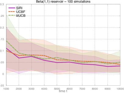
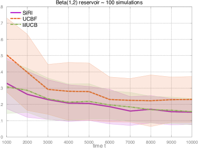
Figure 1: Uniform and ${\rm B}(1,2)$ reservoir distribution

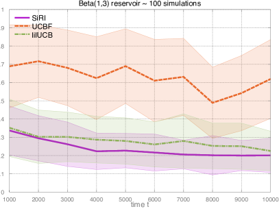
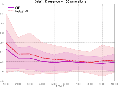
Figure 2: Comparison on ${\rm B}(1,3)$ and unknown $\beta$ on ${\rm B}(1,1)$

Figure 2 also compares SiRI with $\bar{\beta}$-SiRI for the uniform distribution. For this experiment, using $\sqrt{n}$ samples just for the $\beta$ estimation did not decrease the budget too much and at the same time, the estimated $\bar{\beta}$ was precise enough not to hurt the final simple regret.

Conclusion

We presented SiRI, a minimax optimal algorithm for simple regret in infinitely many arms bandit setting, which is interesting when we face enormous number of potential actions. Both the lower and upper bounds give different regimes depending on a complexity $\beta$, a parameter for which we also give an efficient estimation procedure.

Acknowledgments

This work was supported by the French Ministry of Higher Education and Research and the French National Research Agency (ANR) under project ExTra-Learn n.ANR-14-CE24-0010-01.

Appendix A Additional notation

We write $\mathbb{P}_{1}$ for the probability with respect to the arm reservoir distribution, $\mathbb{P}_{2}$ for the probability with respect to the distribution of the samples from the arms, and $\mathbb{P}_{1,2}$ for the probability both with respect to the arm reservoir distribution and the distribution of the samples from the arms.

Let $F$ be the distribution function of the mean reservoir distribution $\mathcal{L}$. Let $F^{-1}$ be the pseudo-inverse of the mean reservoir distribution. In order to express the regularity assumption, we define

$$G\left(\cdot\right)=\bar{\mu}^{*}-F^{-1}\left(1-\cdot\right).$$

We assume that $G$ has a certain regularity in its right end point, which is a standard assumption for infinitely many armed bandits. In particular, we rewrite Assumption 2 by only modifying the constants $\tilde{E},\tilde{E}^{\prime},$ and $\tilde{B}$.

Assumption 3 ($\beta$ regularity in $\bar{\mu}^{*}$, version 2).

Let $\beta>0$. There exist $E,E^{\prime},B\in(0,1)$ such that $\forall u\in[0,B]$,

$$E^{\prime}u^{1/\beta}\geq G\left(u\right)\geq Eu^{1/\beta}.$$

This assumption is equivalent to Assumption 2 which is the same as the classic one (1) by definition of $G$ and $F$ and we reformulate it for the convenience of analysis. Without loss of generality, we assume that $\bar{\mu}^{*}>0$.

Appendix B Full proof of Theorem 2

B.1 Roadmap

The proof of Theorem 2 (upper bounds) is composed of two layers. The first layer consists of proving results on the empirical distributions of the arms emitted by the arms reservoir, the crucial object is event $\xi_{1}$. The second layer consists of proving results on the random samples of the arms, and in particular that the empirical means of the arms are not too different from the true means of the arms. For this part, the crucial object is event $\xi_{2}$. More precisely, these two layers can be decomposed as follows.

• We prove of suitable high probability upper bounds and lower bounds on the number of arms among the $\bar{T}_{\beta}$ arms pulled by the algorithm that have a given gap (with respect to $\bar{\mu}^{*}$), depending on the considered gap. This is done in Lemma 4. Two important results can be consequently deduced: (i) An upper bound on the number of suboptimal arms depending on how suboptimal they are. The more suboptimal they are, the more arms they are, which depends on $\beta$. (ii) A proof that among the $\bar{T}_{\beta}$ arms pulled by the algorithm, there is with high probability at least one arm, and not significantly more than one arm, that has a gap smaller than the simple regret from Theorem 2. This is done in Corollary 3.

• In Lemma 5, we prove that with high probability, the empirical means of the arms are not too different from their true means. The main difficulty is that the means of the arms are random. In order to avoid suboptimal $\log(n)$ dependency in the case $\beta<2$, we use a peeling argument where the peeling is done over these random gaps, using the result from the previous layer, i.e., the bound on the number of arms with a given gap.

Afterwards, we combine the two results to bound the number of suboptimal pulls (section B.5). Since the algorithm pulls the arms depending on the empirical gaps, then (i) the bounds on the number of suboptimal and near-optimal arms, and (ii) the bounds on the deviations of the empirical means with respect to the true means, will allow to obtain the desired bound on the number of suboptimal arms. By construction of the strategy and in particular, by the choice of $\bar{T}_{\beta}$, we prove that with high probability, the number of pulls of the optimal arms is smaller than a fraction of $n$. This means that there is a near-optimal arm that is pulled more than $n/2$ times. This is the one selected by the algorithm which concludes the proof.

B.2 Concentration inequalities

We make several uses of Bernstein’s inequality:

Lemma 2 (Bernstein’s inequality).

Let $\mathbb{E}(X_{t})=0,|X_{t}|\leq b>0$, and $\mathbb{E}(X_{t}^{2})\leq v>0$. Then for any $\delta>0$, with probability at least $1-\delta$

$$\sum_{t=1}^{n}X_{t}\leq\sqrt{2nv\log\delta^{-1}}+\tfrac{b}{3}\log\delta^{-1}$$

Furthermore, Algorithm 2 along with Corollary 1 are based on the empirical Bernstein concentration inequality.

Lemma 3 (Empirical Bernstein’s inequality).

Let $\mathbb{E}(X_{t})=0,|X_{t}|\leq b>0$. Let for any $j=1,\dots,n$

$$V_{j}=\frac{1}{j}\sum_{t=1}^{j}\left(X_{t}-\frac{1}{j}\sum_{i=1}^{j}X_{i}\right)^{2}$$

Then for any $\delta>0$, with probability at least $1-\delta$

$$\sum_{t=1}^{j}X_{t}\leq\sqrt{2nV_{j}\log\left(3\delta^{-1}\right)}+3b\log\left(3\delta^{-1}\right)$$

B.3 Notation

For any $i\leq K_{n}$, set

$$\Delta_{i}=\bar{\mu}^{*}-\mu_{i},$$

where we remind the reader that $\mu_{i}$ is the mean of distribution of arm $i$.

Without loss of generality, we assume that $\bar{\mu}^{*}>0$. For any $u\in\mathbb{N}$, we define

$$I_{u}=\left[\bar{\mu}^{*}-G\left(2^{-u}\right),\bar{\mu}^{*}-G\left(2^{-u-1}\right)\right].$$

We also define

$$I_{-1}=\left[0,\bar{\mu}^{*}-G\left(B\right)\right].$$

We further define

$$I^{*}=\left[\bar{\mu}^{*}-G\left(2^{-\bar{t}_{\beta}}\right),\bar{\mu}^{*}-G\left(0\right)\right]=\left[\bar{\mu}^{*}-G\left(2^{-\bar{t}_{\beta}}\right),\bar{\mu}^{*}\right].$$

Let $N_{u}$ be the number of arms in segment $I_{u}$,

$$N_{u}=\sum_{k=1}^{\bar{T}_{\beta}}\textbf{1}\{\mu_{k}\in I_{u}\},$$

and let $\bar{N}^{*}$ be the number of arms in the segment $I^{*}$,

$$\bar{N}^{*}=\sum_{k=1}^{\bar{T}_{\beta}}\textbf{1}\{\mu_{k}\in I^{*}\}.$$

B.4 Favorable high-probability event

Let $\xi_{1}$ be the event defined as

$$\xi_{1} =\Bigg{\{}\omega:\forall u\in\mathbb{N},u\leq\bar{t}_{\beta},\left|N_{u}-2^{\bar{t}_{\beta}-u-1}\right|\leq\sqrt{(\bar{t}_{\beta}-u+1)2^{\bar{t}_{\beta}-u}\log(1/\delta)}+(\bar{t}_{\beta}-u+1)\log(1/\delta),$$

$$\qquad\qquad\qquad\mathrm{\ and\ }\bar{N}^{*}\leq 1+2\sqrt{\log(1/\delta)}+2\log(1/\delta)\Bigg{\}}$$

$$=\Bigg{\{}\omega:\forall u\in\mathbb{N},u\leq\bar{t}_{\beta},\left|N_{u}-2^{\bar{t}_{\beta}-u-1}\right|\leq 2^{\bar{t}_{\beta}-u-1}\varepsilon_{u}\mathrm{\ and\ }\bar{N}^{*}\leq 1+\varepsilon_{\bar{t}_{\beta}}\Bigg{\}}.$$

where $\varepsilon_{u}=2\sqrt{(\bar{t}_{\beta}-u+1)2^{-(\bar{t}_{\beta}-u)}\log(1/\delta)}+2(\bar{t}_{\beta}-u+1)2^{-(\bar{t}_{\beta}-u)}\log(1/\delta)$.

Lemma 4.

The probability of $\xi_{1}$ under both the distribution of the arm reservoir and the samples of the arms is larger than $1-\left(1+\frac{e}{e-1}\right)\delta$ for $\delta$ small enough,

$$\mathbb{P}_{1}(\xi_{1})=\mathbb{P}_{1,2}\left(\xi_{1}\right)\geq 1-\left(1+\frac{e}{e-1}\right)\delta.$$

Proof of Lemma 4.

Let $u\in\mathbb{N}$. We have by definition that

$$N_{u}=\sum_{k=1}^{\bar{T}_{\beta}}\textbf{1}\{\mu_{k}\in I_{u}\},$$

is a sum of independent Bernoulli random variables of parameter $2^{-u}-2^{-u-1}=2^{-u-1}$. By a Bernstein concentration inequality (Lemma 2) for sums of Bernoulli random variables, this implies that with probability $1-\delta_{u}>0$,

$$\left|N_{u}-2^{\bar{t}_{\beta}-u-1}\right|\leq\sqrt{2^{\bar{t}_{\beta}-u}\log\delta_{u}^{-1}}+\log\delta_{u}^{-1}.$$

Set $\delta_{u}=\exp\left(-\left(\bar{t}_{\beta}-u+1\right)\right)\delta$. Notice that for $u\leq\bar{t}_{\beta}$, $\log\delta_{u}^{-1}\leq(\bar{t}_{\beta}-u+1)\log\delta^{-1}$. Then the result holds by a union bound since for $\delta$ small enough

$$\sum_{u=0}^{\bar{t}_{\beta}}\delta_{u}=\delta\sum_{u=0}^{\bar{t}_{\beta}}\exp\left(-\left(\bar{t}_{\beta}-u+1\right)\right)\leq\frac{e\delta}{e-1},$$

and by similar argument for $\bar{N}^{*}$ which together with another union bound give the claim. ∎

The following corollary follows from Lemma 4.

Corollary 3.

Set $\bar{t}^{*}=\lfloor\bar{t}_{\beta}-96\log_{2}(\log_{2}(\log(1/\delta)))-\log_{2}(\log(1/\delta))\rfloor-2$. Let $\delta$ be smaller than an universal constant. If $n$ is large enough so that $\bar{t}^{*}\geq\log_{2}(1/B)$, then on $\xi_{1}$, there is at least an arm of index in $\{1,\ldots,\bar{T}_{\beta}\}$ such that it belongs to $I_{\bar{t}^{*}}$. If $k^{*}$ is its index, then

$$\Delta_{k^{*}}\leq\tfrac{1}{4}E^{\prime}(\log_{2}(\log(1/\delta)))^{96}2^{-\bar{t}_{\beta}/\beta}\log(1/\delta).$$

Proof of Corollary 3.

First we have for $u\leq\bar{t}^{*}$

$$\varepsilon_{u} =2\sqrt{(\bar{t}_{\beta}-u+1)2^{-(\bar{t}_{\beta}-u)}\log(1/\delta)}+2(\bar{t}_{\beta}-u+1)2^{-(\bar{t}_{\beta}-u)}\log(1/\delta)$$

$$\leq 2\sqrt{\frac{(1+\log_{2}(\log(1/\delta))+96\log_{2}(\log_{2}(\log(1/\delta))))}{96\log_{2}(\log(1/\delta))}}+\frac{2(1+\log_{2}(\log(1/\delta))+96\log_{2}(\log_{2}(\log(1/\delta))))}{96\log_{2}(\log(1/\delta))}$$

$$\leq 4\sqrt{1/(96\log_{2}(\log(1/\delta)))+1/96+\log_{2}(\log_{2}(\log(1/\delta)))/\log_{2}(\log(1/\delta))}$$

$$\leq 1/2,$$

for $\delta$ being a small enough constant.

This implies that for $u\leq\bar{t}^{*}$

$$2^{\bar{t}_{\beta}-u-1}(1-\varepsilon_{u})\geq 2^{2-1}\times 1/2\geq 1.$$

This implies that on $\xi_{1}$, $N_{\bar{t}^{*}}\geq 1$, which means there is at least one arm in $I_{\bar{t}^{*}}$. Let us call $k$ one of these arms. By definition of $I_{\bar{t}^{*}}$, it satisfies

$$\Delta_{k^{*}}\leq G(2^{-\bar{t}^{*}})\leq E^{\prime}2^{-\bar{t}^{*}/\beta}\leq\tfrac{1}{4}E^{\prime}(\log_{2}(\log(1/\delta)))^{96}2^{-\bar{t}_{\beta}/\beta}\log(1/\delta).$$

because of Assumption 3, since $t^{*}\geq\log_{2}(1/B)$. ∎

Let for any $k\in\mathbb{N},1\leq k\leq\bar{T}_{\beta}$

$$n_{k}=\left\lfloor\log_{2}\left(\frac{D\log\left(\max(1,2^{2\bar{t}_{\beta}/b}\Delta_{k}^{2})/b\right)}{\max\left(2^{-2\bar{t}_{\beta}/b},\Delta_{k}^{2}\right)}\right)\right\rfloor,$$

where $D$ is a large constant, and

$$\tilde{n}_{u}=\log_{2}\left(\frac{D\log\left(\max\left(1,2^{2\bar{t}_{\beta}/b}G\left(2^{-\left(u+1\right)}\right)^{2}\right)/\delta\right)}{\max\left(2^{-2\bar{t}_{\beta}/b},G\left(2^{-(u+1)}\right)^{2}\right)}\right).$$

Let also

$$\tilde{n}_{-1}=\log_{2}\left(\frac{D\log\left(\max(1,2^{2\bar{t}_{\beta}/b}G\left(B\right)^{2})/\delta\right)}{\max\left(2^{-2\bar{t}_{\beta}/b},G\left(B\right)^{2}\right)}\right).$$

$$\mathrm{Let\ }\xi_{2}=\left\{\omega:\forall k\in\mathbb{N}^{*},k\leq\bar{T}_{\beta},\forall v\leq n_{k}\left|\frac{1}{2^{v}}\sum_{i=1}^{2^{v}}X_{k,i}-\mu_{k}\right|\leq 2\sqrt{C2^{-v}\log(2^{2\bar{t}_{\beta}/b-v}/\delta)}+2C2^{-v}\log(2^{2\bar{t}_{\beta}/b-v}/\delta)\right\}.$$

Lemma 5.

Case $\beta<2$: Knowing $\xi_{1}$, the probability of $\xi_{2}$ is larger than $1-H\log(1/\delta)^{2}\delta$,

$$\mathbb{P}_{2}\left(\xi_{2}|\xi_{1}\right)\geq 1-H\log\left(1/\delta\right)^{2}\delta,$$

where $H$ is a constant that depends only on $D,E,E^{\prime},\beta$.

Case $\beta\geq 2$: Knowing $\xi_{1}$, the probability of $\xi_{2}$ is larger than $1-H\log(1/\delta)^{2}\log(n)\delta$,

$$\mathbb{P}_{2}\left(\xi_{2}|\xi_{1}\right)\geq 1-H\log(1/\delta)^{2}\log(n)^{2}\delta,$$

where $H$ is a constant that depends only on $D,E,E^{\prime},\beta$.

Proof of Lemma 5.

Let $(k,v)\in\mathbb{N}^{*}\times\mathbb{N}$. Since $(X_{k,i})_{i}$ are i.i.d. from distribution bounded by $C$, we have that with probability (according to the samples) larger than $1-\delta_{k,v}$,

$$\left|\frac{1}{2^{v}}\sum_{i=1}^{2^{v}}X_{k,i}-\mu_{k}\right|\leq\sqrt{2C2^{-v}\log\left(1/\delta_{k,v}\right)}+2C\times 2^{-v}\log\left(1/\delta_{k,v}\right).$$

Set $\delta_{k,v}=2^{v}2^{-2\bar{t}_{\beta}/b}\delta$. We have

$$\sum_{k\leq\bar{T}_{\beta}}\sum_{v\leq n_{k}}\delta_{k,v} =2^{-2\bar{t}_{\beta}/b}\delta\sum_{k\leq\bar{T}_{\beta}}\sum_{v\leq n_{k}}2^{v}\leq 2\times 2^{-2\bar{t}_{\beta}/b}\delta\sum_{k\leq T_{\beta}}2^{n_{k}}\leq 2\times 2^{-2\bar{t}_{\beta}/b}\delta\sum_{u=0}^{\infty}N_{u}2^{\tilde{n}_{u}},$$

since $2^{\tilde{n}_{u}}$ is increasing in $u$.

Again, since $2^{\tilde{n}_{u}}$ is increasing in $u$, is implies that on $\xi_{1}$,

$$\sum_{k\leq\bar{T}_{\beta}}\sum_{v\leq n_{k}}\delta_{k,v} \leq 2\times 2^{-2\bar{t}_{\beta}/b}\delta\sum_{u=0}^{\infty}N_{u}2^{\tilde{n}_{u}}$$

$$\leq 2\times 2^{-2\bar{t}_{\beta}/b}\delta\left(\bar{T}_{\beta}2^{\tilde{n}_{-1}}+\sum_{u=\lfloor\log_{2}(1/B)\rfloor+1}^{\bar{t}_{\beta}}N_{u}2^{\tilde{n}_{u}}+\bar{N}^{*}2^{\tilde{n}_{\bar{t}_{\beta}}}\right)$$ (7)

$$\leq 2\times 2^{-2\bar{t}_{\beta}/b}\delta\left(\frac{\bar{T}_{\beta}D\log(2^{2\bar{t}_{\beta}/b}E^{\prime}B^{-2/\beta}/\delta)}{EB^{-2/\beta}}+\!\!\!\!\!\!\!\!\!\sum_{u=\lfloor\log_{2}(1/B)\rfloor+1}^{\bar{t}_{\beta}}\!\!\!\!\!\!\!\!\!\frac{N_{u}D\log(2^{2\bar{t}_{\beta}/b}G(2^{-(u+1)})^{2}/\delta)}{G(2^{-(u+1)})^{2}}+\bar{N}^{*}D\log\left(\tfrac{1}{\delta}\right)2^{2\bar{t}_{\beta}/b}\right)$$

$$\leq 2\times 2^{-2\bar{t}_{\beta}/b}\delta\left(\frac{2^{\bar{t}_{\beta}}DE^{\prime}\log\left(\tfrac{n}{\delta}\right)}{E}+\!\!\!\!\!\!\!\!\!\!\sum_{u=\lfloor\log_{2}(1/B)\rfloor+1}^{\bar{t}_{\beta}}\!\!\!\!\!\!\!\!\!\!\!\!2^{\bar{t}_{\beta}\!-\!u\!-1\!}(1+\varepsilon_{u})\frac{D\log\left(\tfrac{E}{\delta}\right)\left(\frac{2\bar{t}_{\beta}}{b}\!-\!\frac{2(u\!-\!1)}{\beta}\right)}{E2^{-2(u-1)/\beta}}+(1+\varepsilon_{\bar{t}_{\beta}})D\log\left(\tfrac{1}{\delta}\right)2^{2\bar{t}_{\beta}/b}\right)$$

$$\leq 2\times 2^{-2\bar{t}_{\beta}/b}\delta\left(\frac{2^{\bar{t}_{\beta}}DE^{\prime}\log\left(\tfrac{n}{\delta}\right)}{E}+\sum_{u=0}^{\bar{t}_{\beta}}6D/(Eb)\log\left(\tfrac{E}{\delta}\right)^{2}2^{\bar{t}_{\beta}-u+2u/\beta}(2\bar{t}_{\beta}-2(u-1))+5D\log\left(\tfrac{1}{\delta}\right)^{2}2^{2\bar{t}_{\beta}/b}\right),$$

since $\varepsilon_{u}\leq 4(\bar{t}_{\beta}-u+1)\log\left(\tfrac{1}{\delta}\right)$ and since $b\leq\beta$, which implies that $2\bar{t}_{\beta}-2(u-1)\geq 1$.

Case 1: $\beta<2$:

In this case, $b=\beta$. Since $\sum_{u=0}^{\infty}2^{-u/v}u^{v^{\prime}}<\infty$ for any $v,v^{\prime}>0$ that on $\xi_{1}$, the last equation implies

$$\sum_{k\leq\bar{T}_{\beta}}\sum_{v\leq n_{k}}\delta_{k,v}\leq 2\times 2^{-2\bar{t}_{\beta}/\beta}\delta\left(\frac{2^{\bar{t}_{\beta}}DE^{\prime}\log\left(\tfrac{n}{\delta}\right)}{E}+\frac{3DF_{1}^{\prime}}{E\beta}\log\left(\tfrac{E}{\delta}\right)2^{2\bar{t}_{\beta}/\beta}+5D\log\left(\tfrac{1}{\delta}\right)^{2}2^{2\bar{t}_{\beta}/\beta}\right)\leq F_{1}\log\left(\tfrac{1}{\delta}\right)^{2}\delta,$$

where $F_{1}^{\prime},F_{1}>0$ are constants.

Case 2: $\beta>2$:

In this case, $b=2$. Since $\sum_{u=0}^{\infty}2^{-u/v}<\infty$ for any $v>0$ that on $\xi_{1}$, the last equation implies

$$\!\!\!\!\!\!\!\!\!\!\!\!\!\!\!\!\!\!\!\!\!\!\!\!\!\!\!\!\!\!\!\!\!\!\!\!\!\!\!\!\!\!\!\!\!\!\!\!\sum_{k\leq\bar{T}_{\beta}}\sum_{v\leq n_{k}}\delta_{k,v} \leq 2\times 2^{-\bar{t}_{\beta}}\delta\left(\frac{2^{\bar{t}_{\beta}}DE^{\prime}\log\left(\tfrac{n}{\delta}\right)}{E}+\frac{3DF_{2}^{\prime}}{E\beta}\log\left(\tfrac{E}{\delta}\right)^{2}2^{\bar{t}_{\beta}}t_{\beta}+5D\log\left(\tfrac{1}{\delta}\right)^{2}2^{\bar{t}_{\beta}}\right)$$

$$\leq F_{2}\log\left(\tfrac{1}{\delta}\right)^{2}\bar{t}_{\beta}\delta\leq F_{2}\log\left(\tfrac{1}{\delta}\right)^{2}\log(n)\delta,$$

where $F_{2}^{\prime},F_{2}>0$ are constants.

Case 3: $\beta=2$:

In this case, we have on $\xi_{1}$

$$\sum_{k\leq\bar{T}_{\beta}}\sum_{v\leq n_{k}}\delta_{k,v} \leq 2\times 2^{-\bar{t}_{\beta}}\delta\left(\frac{2^{\bar{t}_{\beta}}DE^{\prime}\log\left(\tfrac{n}{\delta}\right)}{E}+\sum_{u=0}^{\bar{t}_{\beta}}\frac{3D}{E\beta}\log\left(\tfrac{E}{\delta}\right)^{2}2^{\bar{t}_{\beta}}(2\bar{t}_{\beta}-2(u-1))+5D\log\left(\tfrac{1}{\delta}\right)^{2}2^{\bar{t}_{\beta}}\right)$$

$$\leq F_{3}\log\left(\tfrac{1}{\delta}\right)^{2}\bar{t}_{\beta}^{2}\delta\leq F_{3}\log\left(\tfrac{1}{\delta}\right)^{2}\log(n)^{2}\delta.$$

where $F_{3}>0$ is a constant. ∎

Let $\xi=\xi_{1}\cap\xi_{2}.$ By Lemmas 4 and 5, we know that for a given constant $F_{4}$ that depends only on $\beta,D,E,E^{\prime}$,

• Case $\beta<2$:

  $$\mathbb{P}(\xi)\geq 1-F_{4}\log\left(\tfrac{1}{\delta}\right)^{2}\delta.$$

• Case $\beta\geq 2$:

  $$\mathbb{P}(\xi)\geq 1-F_{4}\log\left(\tfrac{1}{\delta}\right)^{2}\log(n)^{3}\delta.$$

B.5 Upper bound on the number of pulls of the non-near-optimal arms

Let $k$ be an arm such that $k\leq\bar{T}_{\beta}$, and $t\leq n$ be a time. On the event $\xi$, by definition, we have

$$\left|\widehat{\mu}_{k,t}-\mu_{k}\right|\leq 2\sqrt{\frac{C\log\big{(}2^{2\bar{t}_{\beta}/b}/(T_{k,t}\delta)\big{)}}{T_{k,t}}}+\frac{2C\log\big{(}2^{2\bar{t}_{\beta}/b}/(T_{k,t}\delta)\big{)}}{T_{k,t}},$$

which implies by definition of the upper confidence bound that on $\xi$

$$\mu_{k}\leq B_{k,t}\leq\mu_{k}+\varepsilon_{k,t},\quad\mathrm{where}\quad\varepsilon_{k,t}=2\sqrt{\frac{C\log\left(2^{2\bar{t}_{\beta}/b}/(T_{k,t}\delta)\right)}{T_{k,t}}}+\frac{2C\log\left(2^{2\bar{t}_{\beta}/b}/(T_{k,t}\delta)\right)}{T_{k,t}}.$$ (8)

Let us now write $k^{*}$ for the best arm among the ones in $\{1,\ldots,T_{\beta}\}$. Note that $k^{*}$ may be different from the best possible arm. By Corollary 3, we know that on $\xi$, $k^{*}$ satisfies

$$\Delta_{k^{*}}\leq\tfrac{1}{4}E^{\prime}\left(\log_{2}\left(\log\left(1/\delta\right)\right)\right)^{96}2^{-\bar{t}_{\beta}/\beta}\log\left(\tfrac{1}{\delta}\right)=\varepsilon^{*}.$$

Arm $k$ is pulled at time $t$ instead of $k^{*}$ only if

$$B_{k,t}\geq B_{k^{*},t}.$$

On $\xi$, this happens if

$$\bar{\mu}^{*}-\varepsilon^{*}\leq\mu_{k}+\varepsilon_{k,t},$$

which happens if (on $\xi$)

$$\Delta_{k}-\varepsilon^{*}\leq\varepsilon_{k,t},$$

and if we assume that $\Delta_{k}\geq 2\varepsilon^{*}$, it implies that on $\xi$ arm $k$ is pulled at time $t$ only if

$$\Delta_{k}\leq 2\varepsilon_{k,t}.$$ (9)

We define $u$ such that (i) that $\mu_{k}\in I_{u}$ if $u\geq\lfloor\log_{2}(B)\rfloor+1$ or (ii) $u=-1$ otherwise. Assume that

$$T_{k,t}\geq 2^{\tilde{n}_{u}}\geq\frac{D\log\left(\max\left(1,2^{2\bar{t}_{\beta}/b}G\left(2^{-\left(u+1\right)}\right)^{2}\right)/\delta\right)}{\max\left(2^{-2\bar{t}_{\beta}/b},G\left(2^{-\left(u+1\right)}\right)^{2}\right)} \geq\frac{D\log(2^{2\bar{t}_{\beta}/b}G(2^{-(u+1)})^{2}/\delta)}{G(2^{-(u+1)})^{2}},$$

since we assumed that $\Delta_{k}\geq 2\varepsilon^{*}$, which implies that $t_{k,t}\leq t^{*}\leq\bar{t}_{\beta}$.

By Assumption 3, and since $\mu_{k}\in I_{u}$, we know that $G(2^{-(u+1)})\leq\Delta_{k}$. Therefore, the last equation implies

$$T_{k,t}\geq 2^{\tilde{n}_{u}}\geq\frac{D\log\left(\max\left(1,2^{2\bar{t}_{\beta}/b}G\left(2^{-\left(u+1\right)}\right)^{2}\right)/\delta\right)}{\max\left(2^{-2\bar{t}_{\beta}/b},G\left(2^{-\left(u+1\right)}\right)^{2}\right)} \geq\frac{D\log\left(2^{2\bar{t}_{\beta}/b}\Delta_{k}^{2}/\delta\right)}{\Delta_{k}^{2}}.$$

For such a $T_{k,t}$, we have

$$\frac{\log\left(2^{2\bar{t}_{\beta}/b}/\left(T_{k,t}\delta\right)\right)}{T_{k,t}} \leq\frac{\Delta_{k}^{2}\log\left(D2^{2\bar{t}_{\beta}/b}\Delta_{k}^{2}/\delta\right)}{D\log\left(2^{2\bar{t}_{\beta}/b}\Delta_{k}^{2}/\delta\right)}\leq\frac{\Delta_{k}^{2}\log D}{D}\leq\Delta_{k}^{2}/(16C),$$

for $D$ large enough so that $D\geq 32(C+1)\log(32(C+1))$. Therefore, by definition of $\varepsilon_{k},t$, the last equation implies that for $T_{k,t}\geq 2^{\tilde{n}_{u}}$, we have

$$\varepsilon_{k,t}\leq\Delta_{k}/4.$$

The last equation implies together with (9) that if $T_{k,t}\geq 2^{\tilde{n}_{u}}$, then on $\xi$, arm $k$ is not pulled from time $t$ onwards. In particular, this implies that on $\xi$

$$T_{k,n}\leq 2^{\tilde{n}_{u}},$$

for any $k\leq\bar{T}_{\beta}$ such that $\Delta_{k}\geq 2\varepsilon^{*}$, and such that (i) $\mu_{k}\in I_{u}$ if $u\geq\lfloor\log_{2}(B)\rfloor+1$ or (ii) or $u=-1$ otherwise.

Let $\mathcal{A}$ be the set of arms such that $\Delta_{k}\geq 2\varepsilon^{*}$. From the previous equation, the number of times that they are pulled is bounded on $\xi$ as

$$\sum_{k\in\mathcal{A}}T_{k,n}\leq\sum_{u\leq\bar{t}_{\beta}}N_{u}2^{\tilde{n}_{u}}\leq\bar{T}_{\beta}2^{\tilde{n}_{-1}}+\!\!\!\!\!\!\!\!\sum_{\lfloor\log_{2}(B)\rfloor\leq u\leq\bar{t}_{\beta}}N_{u}2^{\tilde{n}_{u}}.$$

Bounding this quantity can be done in essentially the same way as in (7). We again obtain three cases,

• Case 1: $\beta<2$: In this case on $\xi$

  $$\sum_{k\in\mathcal{A}}T_{k,n} \leq\frac{2^{\bar{t}_{\beta}}DE^{\prime}\log(n/\delta)}{E}+\frac{3DF_{1}^{\prime}}{E\beta}\log(E/\delta)^{2}2^{2\bar{t}_{\beta}/\beta}\leq n/H,$$

  where $H$ is arbitrarily large for $A$ small enough in the definition of $\bar{T}_{\beta}$.

• Case 2: $\beta>2$: In this case on $\xi$

  $$\sum_{k\in\mathcal{A}}T_{k,n} \leq\frac{2^{\bar{t}_{\beta}}DE^{\prime}\log(n/\delta)}{E}+\frac{3DF_{2}^{\prime}}{E\beta}\log(E/\delta)^{2}2^{\bar{t}_{\beta}}t_{\beta}\leq n/H,$$

  where $H$ is arbitrarily large for $A$ small enough in the definition of $\bar{T}_{\beta}$.

• Case 3: $\beta=2$: In this case on $\xi$

  $$\sum_{k\in\mathcal{A}}T_{k,n} \leq\frac{2^{\bar{t}_{\beta}}DE^{\prime}\log(n/\delta)}{E}+\sum_{u=0}^{\bar{t}_{\beta}}\frac{3D}{E\beta}\log(E/\delta)^{2}2^{\bar{t}_{\beta}}(2\bar{t}_{\beta}-2(u-1))\leq n/H,$$

  where $H$ is arbitrarily large for $A$ small enough in the definition of $\bar{T}_{\beta}$.

Consider now $u^{*}$ such that $u^{*}=\lfloor\log_{2}\big{(}1/\bar{F}(\varepsilon^{*})\big{)}\rfloor$. By definition of $\varepsilon^{*}$, we know that on $\xi$, we have

$$u^{*}\geq t^{*}-\upsilon(\delta)$$

Therefore with high probability, by Lemma 4 and as in Corollary 3, on $\xi$, there are less than $N(\delta)$ arms of index smaller than $\bar{T}_{\beta}$ such that $\Delta_{k}\leq 2\varepsilon^{*}$, where $N(\delta)$ is a constant that depends only on $\delta$. For $H$ large enough, on $\xi$, $N(\delta)\leq H$. This implies, together with the three cases, that there is at least an arm of index smaller than $\bar{T}_{\beta}$ and such that $\Delta_{k}\leq 2\varepsilon^{*}$ that is pulled more than $n/H$ times. This implies that the most pulled arm is such that, on $\xi$, $\Delta_{k}\leq 2\varepsilon^{*}$. This implies that the regret is on $\xi$ bounded as

$$r_{n}\leq\frac{E^{\prime}(\log_{2}(\log(1/\delta)))^{96}}{4}2^{-\bar{t}_{\beta}/\beta}\log(1/\delta)\leq E^{\prime\prime}n^{b/(2\beta)}A(n)^{1/\beta}(\log(\log(1/\delta)))^{96}\log(1/\delta)$$

Therefore, by Lemmas 4 and 5, the previous equation implies in the three cases for some constants $E_{4},E^{\prime\prime\prime}$:

• Case $\beta<2$: With probability larger than $1-F_{4}\log(1/\delta)^{2}\delta$, we have

  $$r_{n} \leq E^{\prime\prime\prime}n^{-1/2}(\log(\log(1/\delta)))^{96}\log(1/\delta),$$

  hence with probability larger than $1-\delta$,

  $$r_{n} \leq E_{4}n^{-1/2}\log(1/\delta)(\log(\log(1/\delta)))^{96}\sim n^{-1/2}.$$

• Case $\beta>2$: With probability larger than $1-F_{4}\log(1/\delta)^{2}\log(n)^{3}\delta$, we have

  $$r_{n} \leq E^{\prime\prime\prime}(n\log(n))^{-1/\beta}(\log(\log(1/\delta)))^{96}\log(1/\delta),$$

  hence with probability larger than $1-\delta$,

  $$r_{n} \leq E_{4}(n\log(n))^{-1/\beta}(\log(\log(\log(n)/\delta)))^{96}\log(\log(n)/\delta)\sim(n\log(n))^{-1/\beta}\log\log(n)\log\log\log(n)^{96}.$$

• Case $\beta=2$: With probability larger than $1-F_{4}\log(1/\delta)^{2}\log(n)^{3}\delta$, we have

  $$r_{n} \leq E^{\prime\prime\prime}\log(n)n^{-1/2}(\log(\log(1/\delta)))^{96}\log(1/\delta),$$

  hence with probability larger than $1-\delta$,

  $$r_{n} \leq E_{4}\log(n)n^{-1/2}(\log(\log(\log(n)/\delta)))^{96}\log(\log(n)/\delta)\sim\log(n)n^{-1/2}\log\log(n)\log\log\log(n)^{96}.$$

Appendix C Full proof of Theorem 1

C.1 Case $\beta<2$

By Assumption 2 (equivalent to Assumption 3), we know that

$$E^{\prime}u^{1/\beta}\geq G(u)\geq Eu^{1/\beta}.$$

Assume that when pulling an arm from the reservoir, its distribution is Gaussian of mean following the distribution associated to $G$ and has variance $1$. Since the budget is bounded by $n$, an algorithm pulls at most $n$ arms from the arm reservoir. Let us define

$$I_{1}=\left[\bar{\mu}^{*}-\frac{E^{\prime}c_{1}^{1/\beta}}{\sqrt{n}},\bar{\mu}^{*}-\frac{E(c_{1}^{\prime})^{1/\beta}}{\sqrt{n}}\right]\quad\mathrm{and}\quad I_{2}=\left[\bar{\mu}^{*}-\frac{E(c_{1}^{\prime})^{1/\beta}}{\sqrt{n}},\bar{\mu}^{*}\right],$$

where $c_{1},c_{1}^{\prime}$ are constants. If we denote $N_{1}$ the number of arms in $I_{1}$ and $N_{2}$ the number of arms in $I_{2}$ among the $n$ first arms pulled from the arm reservoir, we can use Bernstein’s inequality and for $n\geq 1$ larger than a large enough constant

$$\mathbb{P}_{1}\left(N_{2}\geq n\frac{E^{\prime}/Ec_{1}^{\prime}}{n^{\beta/2}}\left(1+\log\left(1/\delta\right)\right)\right)\leq\delta\quad\mathrm{and}\quad\mathbb{P}_{1}\left(N_{1}\leq n\frac{c_{1}-c_{1}^{\prime}}{n^{\beta/2}}\left(1-\log\left(1/\delta\right)\right)\right)\leq\delta.$$

Consequently, for $c_{1}$ large enough when compared to $c^{\prime}_{1}$, it implies that with probability larger than $1-2\delta$, we have that $N_{1}>1$ and $N_{1}>N_{2}$. Consider the event $\xi$ of probability $1-2\delta$ where this is satisfied.

On $\xi$, a problem that is strictly easier than the initial problem is the one where an oracle points out two arms to the learner, the best arm in $I_{2}$ and the worst arm in $I_{1}$, and where the objective is to distinguish between these two arms and output the arm in $I_{2}$. Indeed, this problem is on $\xi$ strictly easier than an intermediate problem where an oracle provides the set of arms in $I_{1}\cup I_{2}$ and asks for an arm in $I_{2}$, since $N_{1}>N_{2}$. On $\xi$, this intermediate problem is in turn strictly easier than the original problem of outputting an arm in $I_{2}$ without oracle knowledge. Therefore, for the purpose of constructing the lower bound, we will now turn to the strictly easier problem of deciding between the arm $k^{*}$ with highest mean in $I_{2}$, and the arm $k$ with lowest mean in $I_{1}$ and prove the lower bound for this strictly easier problem.

Since the number of pulls on both $k^{*}$ and $k$ is bounded by $n$, we use the chain rule and the fact that the distributions are Gaussian to get on $\xi$

$${\rm KL}(k,k^{*})\leq n(\mu-\mu^{*})^{2},$$

where $\mu$ is the mean of $k$ and $\mu^{*}$ is the mean of $k^{*}$. Given $\xi$, let $p$ be the probability that $k$ is selected as the best arm, and $p^{*}$ the probability that $k^{*}$ is selected as the best arm. By Pinsker’s inequality, we know that on $\xi$

$$\left|p-p^{*}\right|\leq\sqrt{{\rm KL}(k_{1},k^{*})}\leq\sqrt{n}|\mu_{1}-\bar{\mu}^{*}|\leq\sqrt{n}E^{\prime}\frac{c_{1}^{1/\beta}}{\sqrt{n}}\leq E^{\prime}c_{1}^{1/\beta}.$$

Since there are only two arms in this simplified game, we know that on $\xi$

$$p^{*}\leq 1/2+E^{\prime}c_{1}^{1/\beta}\leq 7/12.$$

for $c_{1}$ small enough. By definition of $\xi$ and since the problem we considered is easier than the initial problem, we know that for all algorithms, the probability $P^{*}$ of selecting an arm in $I_{2}$ is bounded as follows where we add the probability that $\xi$ does not hold,

$$P^{*}\leq 7/12+2\delta\leq 2/3,$$

for $\delta$ small enough. This concludes the proof by definition of $I_{2}$.

C.2 Case $\beta\geq 2$

By Assumption 2 (equivalent to Assumption 3), we know that

$$E^{\prime}u^{1/\beta}\geq G(u)\geq Eu^{1/\beta}.$$

Assume that when pulling an arm from the reservoir, its distribution is Gaussian of mean following the distribution associated to $G$ and has a variance $1$. The total number of arms pulled in the reservoir is smaller than $n$ since the budget is bounded by $n$. Let

$$I_{0}=\left[\bar{\mu}^{*}-E\left(\frac{c_{0}}{n}\right)^{1/\beta},\bar{\mu}^{*}\right].$$

where $c_{0}$ is a constant defined in function of $\delta>0$ such that, if we denote $N_{0}$ for the number of arms in $I_{0}$, we have

$$\mathbb{P}_{1}\left(N_{0}=0\right)\geq\left(1-\frac{c_{0}}{n}\right)^{n}\geq\exp\left(-c_{0}/2\right)\geq 1-\delta.$$

Thereupon, there are no arms in $I_{0}$ with probability larger than $1-\delta$, and therefore, with probability larger than $1-\delta$ the regret of the algorithm is larger than

$$E\left(\frac{c_{0}}{n}\right)^{1/\beta}.$$

Appendix D Proof of Lemma 1

By a union bound, we know that with probability larger than $1-\delta$, for all $k\leq N$, we have

$$\left|\widehat{m}_{k}-m_{k}\right|\leq c\sqrt{\frac{\log\left(N/\delta\right)}{N}}.$$

Note that by Assumption 2, we have that with probability larger than $1-\delta$,

$$\left|\widehat{m}^{*}-\bar{\mu}^{*}\right|\leq c\left(\frac{1}{\delta N}\right)^{1/\beta}.$$

Let us write

$$v_{N}=c\sqrt{\frac{\log\left(N/\delta\right)}{N}}+c\left(\frac{1}{\delta N}\right)^{1/\beta}.$$

Note first that with probability larger than $1-\delta$ on the samples (not on $m_{k}$)

$$\frac{1}{N}\sum_{k=1}^{N}\mathbf{1}\{\bar{\mu}^{*}-m_{k}\leq N^{-\varepsilon}+v_{N}\}\geq\widehat{p}\geq\frac{1}{N}\sum_{k=1}^{N}\mathbf{1}\{\bar{\mu}^{*}-m_{k}\leq N^{-\varepsilon}-v_{N}\},$$

We now define for $l\in\{0,1\}$

$$p^{+}=\mathbb{P}_{m\sim\mathcal{L}}\left(\bar{\mu}^{*}-m\leq N^{-\varepsilon}+v_{N}\right)\quad\mathrm{and}\quad p^{-}=\mathbb{P}_{m\sim\mathcal{L}}\left(\bar{\mu}^{*}-m\leq N^{-\varepsilon}-v_{N}\right).$$

Notice that for $n$ larger than a constant that depends on $\tilde{B}$ of Assumption 2, we have by Assumption 2 the following bound for $*\in\{+,-\}$, since $(v_{N}N^{\varepsilon})\leq 1/2\delta^{-1/\beta}$ as $\varepsilon<\min(\beta,1/2)$, and also for $N$ larger than a constant that depends on $\tilde{B}$ only

$$\left|-\frac{\log(p^{*})}{\varepsilon\log N}-\beta\right| \leq\frac{(v_{N}N^{\varepsilon})^{\beta}/\beta+\max(1,\log(\tilde{E}^{\prime}),|\log(\tilde{E})|)}{\varepsilon\log N}\leq\frac{\delta^{-1/\beta}/\beta+\max(1,\log(\tilde{E}^{\prime}),|\log(\tilde{E})|)}{\varepsilon\log N},$$

which implies that

$$p^{*}\geq c^{\prime}N^{-\beta\varepsilon},$$

where $c^{\prime}>1/2$ is a small constant that is larger than $\tilde{E}/2$ for $n$ larger than a constant that depends only on $\tilde{B}$.

By Hoeffding’s inequality applied to Bernoulli random variables, we have that with probability larger than $1-\delta$

$$\left|\frac{1}{N}\sum_{k=1}^{N}\mathbf{1}\{\bar{\mu}^{*}-m_{k}\leq N^{-\varepsilon}+v_{N}\}-p^{+}\right|\leq c\sqrt{\frac{\log(1/\delta)}{N}}\mathop{\overset{\mathrm{def}}{\leavevmode\resizebox{0.0pt}{0.0pt}{=}}}w_{N},$$

and the same for $p^{-}$ with $\frac{1}{N}\sum_{k=1}^{N}\mathbf{1}\{\bar{\mu}^{*}-m_{k}\leq N^{-\varepsilon}-v_{N}\}$. All of this implies that with probability larger than $1-6\delta$

$$p^{+}+w_{N}\geq\widehat{p}\geq p^{-}-w_{N},$$

which implies that with probability larger than $1-6\delta$

$$-\frac{\log(p^{+}+w_{N})}{\varepsilon\log N}\leq\widehat{p}\leq-\frac{\log(p^{-}-w_{N})}{\varepsilon\log N},$$

i.e., with probability larger than $1-6\delta$, since $w_{N}/p^{-}\leq 1/2\sqrt{\log(1/\delta)}$ as $n$ is large enough (larger than a constant) and since $\beta\leq 1/(2\varepsilon)$

$$-\frac{\log(p^{+})}{\varepsilon\log N}-\frac{2w_{N}}{p^{+}\log(n)\varepsilon}\leq-\frac{\log(\widehat{p})}{\varepsilon\log N}\geq-\frac{\log(p^{-})}{\varepsilon\log N}+\frac{2w_{N}}{p^{-}\varepsilon\log N},$$

which implies the final claim

$$\left|-\frac{\log(\widehat{p})}{\varepsilon\log N}-\beta\right|\leq\frac{\delta^{-1/\beta}/\beta+\sqrt{\log(1/\delta)}+\max(1,\log(\tilde{E}^{\prime}),|\log(\tilde{E})|)}{\varepsilon\log N}.$$

References

- Audibert & Bubeck (2009) Audibert, Jean-Yves and Bubeck, Sébastien. Minimax Policies for Adversarial and Stochastic Bandits. In Conference on Learning Theory, 2009.
- Audibert et al. (2007) Audibert, Jean-Yves, Munos, Rémi, and Szepesvári, Csaba. Tuning Bandit Algorithms in Stochastic Environments. In Algorithmic Learning Theory, 2007.
- Audibert et al. (2010) Audibert, Jean-Yves, Bubeck, Sébastien, and Munos, Rémi. Best arm identification in multi-armed bandits. Conference on Learning Theory, 2010.
- Azar et al. (2014) Azar, Mohammad Gheshlaghi, Lazaric, Alessandro, and Brunskill, Emma. Online Stochastic Optimization under Correlated Bandit Feedback. In International Conference on Machine Learning, 2014.
- Berry et al. (1997) Berry, Donald A., Chen, Robert W., Zame, Alan, Heath, David C., and Shepp, Larry A. Bandit problems with infinitely many arms. Annals of Statistics, 25:2103–2116, 1997.
- Bonald & Proutière (2013) Bonald, Thomas and Proutière, Alexandre. Two-Target Algorithms for Infinite-Armed Bandits with Bernoulli Rewards. In Neural Information Processing Systems, 2013.
- Carpentier & Kim (2014) Carpentier, Alexandra and Kim, Arlene K. H. Adaptive and minimax optimal estimation of the tail coefficient. Statistica Sinica, 2014.
- Carpentier & Valko (2015) Carpentier, Alexandra and Valko, Michal. Simple regret for infinitely many armed bandits. ArXiv e-prints, 2015.
- Catoni (2012) Catoni, Olivier. Challenging the empirical mean and empirical variance: a deviation study. In Annales de l’Institut Henri Poincaré, Probabilités et Statistiques, volume 48, pp. 1148–1185, 2012.
- Dani et al. (2008) Dani, Varsha, Hayes, Thomas P, and Kakade, Sham M. Stochastic Linear Optimization under Bandit Feedback. In Conference on Learning Theory, 2008.
- de Haan & Ferreira (2006) de Haan, Laurens and Ferreira, Ana. Extreme Value Theory: An Introduction. Springer Series in Operations Research and Financial Engineering. Springer, 2006.
- Even-Dar et al. (2006) Even-Dar, Eyal, Mannor, Shie, and Mansour, Yishay. Action elimination and stopping conditions for the multi-armed bandit and reinforcement learning problems. The Journal of Machine Learning Research, 7:1079–1105, 2006.
- Gabillon et al. (2012) Gabillon, Victor, Ghavamzadeh, Mohammad, and Lazaric, Alessandro. Best arm identification: A unified approach to fixed budget and fixed confidence. In Neural Information Processing Systems, 2012.
- Hauskrecht et al. (2006) Hauskrecht, Milos, Pelikan, Richard, Valko, Michal, and Lyons-Weiler, James. Feature Selection and Dimensionality Reduction in Genomics and Proteomics. In Berrar, Dubitzky, and Granzow (eds.), Fundamentals of Data Mining in Genomics and Proteomics. Springer, 2006.
- Hill (1975) Hill, Bruce M. A Simple General Approach to Inference About the Tail of a Distribution. The Annals of Statistics, 3(5):1163–1174, 1975.
- Jamieson et al. (2014) Jamieson, Kevin, Malloy, Matthew, Nowak, Robert, and Bubeck, Sébastien. lil’UCB: An Optimal Exploration Algorithm for Multi-Armed Bandits. In Conference on Learning Theory, 2014.
- Kalyanakrishnan et al. (2012) Kalyanakrishnan, Shivaram, Tewari, Ambuj, Auer, Peter, and Stone, Peter. PAC subset selection in stochastic multi-armed bandits. In International Conference on Machine Learning, 2012.
- Karnin et al. (2013) Karnin, Zohar, Koren, Tomer, and Somekh, Oren. Almost optimal exploration in multi-armed bandits. In International Conference on Machine Learning, 2013.
- Kaufmann & Kalyanakrishnan (2013) Kaufmann, Emilie and Kalyanakrishnan, Shivaram. Information complexity in bandit subset selection. In Conference on Learning Theory, 2013.
- Kleinberg et al. (2008) Kleinberg, Robert, Slivkins, Alexander, and Upfal, Eli. Multi-armed bandit problems in metric spaces. In 40th ACM Symposium on Theory Of Computing, 2008.
- Munos (2014) Munos, Rémi. From Bandits to Monte-Carlo Tree Search: The Optimistic Principle Applied to Optimization and Planning. Foundations and Trends in Machine Learning, 7(1):1–130, 2014.
- Pickands (1975) Pickands, James III. Statistical Inference Using Extreme Order Statistics. The Annals of Statistics, 3:119–131, 1975.
- Wang et al. (2008) Wang, Yizao, Audibert, Jean-Yves, and Munos, Rémi. Algorithms for Infinitely Many-Armed Bandits. In Neural Information Processing Systems, 2008.