On the Formation of Circles in Co-authorship Networks

Abstract

The availability of an overwhelmingly large amount of bibliographic information including citation and co-authorship data makes it imperative to have a systematic approach that will enable an author to organize her own personal academic network profitably. An effective method could be to have one’s co-authorship network arranged into a set of “circles”, which has been a recent practice for organizing relationships (e.g., friendship) in many online social networks.

In this paper, we propose an unsupervised approach to automatically detect circles in an ego network such that each circle represents a densely knit community of researchers. Our model is an unsupervised method which combines a variety of node features and node similarity measures. The model is built from a rich co-authorship network data of more than 8 hundred thousand authors. In the first level of evaluation, our model achieves 13.33% improvement in terms of overlapping modularity compared to the best among four state-of-the-art community detection methods. Further, we conduct a task-based evaluation – two basic frameworks for collaboration prediction are considered with the circle information (obtained from our model) included in the feature set. Experimental results show that including the circle information detected by our model improves the prediction performance by $9.87\%$ and $15.25\%$ on average in terms of $AUC$ (Area under the ROC) and $Prec@20$ (Precision at Top 20) respectively compared to the case, where the circle information is not present.

1 Introduction

Now-a-days, public repositories of bibliographic datasets such as DBLP and Google Scholar allow us access to a stream of scientific articles published by authors from different domains. An author, we wish to analyze, might be associated with overwhelming volumes of information in terms of her collaborations and publications, which in turn leads to both information overload and high computational complexity. Moreover from an author’s perspective, it could become painstakingly difficult to keep track of the entire set of academic relationships she has with her collaborators at any point of time.

Present Work: Problem definition. In this article, we study the problem of automatically discovering an author’s academic circles. In particular, given a single author with her co-authorship network, our goal is to identify her circles, each of which is a subset of her coauthors. Some examples of real-world circles in an author’s co-authorship network are shown in Figure 1. The “owner” of such a network (the “ego”) may wish to form circles based on common bonds and attributes among her coauthors (the “alters”). An author could have several reasons behind initiating a new collaboration. Some common tendencies exhibited by authors include collaborations with the people from her own Institute or with people sharing the same research interest with her. Therefore, the problem of deciding upon a single dimension to both characterize the circles and categorize the coauthors appropriately becomes extremely challenging. Moreover, circles are author-specific, as each author organizes her personal network of coauthors independent of all other authors with whom she is not connected. This leads to a problem of designing an automatic method that organizes an author’s academic network, more precisely, categorizes her surrounding neighborhoods into meaningful circles.

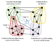
Figure 1: (Color online) A hypothetical example showing an ego network of an author $u$ with labeled circles. Alters might belong to multiple groups and form overlapping circles.

Present Work: Motivation of the work. The problem of detecting ego-centric circles in a co-authorship network is useful in many aspects. The collaborators of a particular researcher might have interests aligned with different topics, and the set of collaborators the researcher is currently working with is a reflection of her current topic of interest. Thus, by understanding circles around her co-authorship network, she might discover that she might be interested in reading papers about a certain topic that she has not been interested in before. This result in turn helps in personalized paper recommendations. On the other hand, if one is interested to start a new collaboration in a particular field with very famous researcher (usually having less opportunity for new collaboration), a more successful attempt could be to first establish a collaboration to one of the coauthors of the famous researcher who happens to belong to a circle that is most aligned to the field of interest. Therefore, the circle information could lead to the design of a meaningful collaboration prediction system. Moreover, one can also discover the collaboration pattern of a researcher by observing the temporal evolution of the ego-centric circles of an author.

Present Work: An unsupervised approach for circle detection. In this work, we propose an unsupervised method to learn the major dimensions of author profile similarity that lead to densely linked circles. In practice, since the topological evidence in such small ego networks is less, the traditional community finding algorithms fail to discover meaningful circles from it [15, 16]. Here, we intend the following two conditions to be satisfied during circle detection: first, we expect the circles to be formed by densely connected sets of alters. Different circles might overlap, i.e., alters might belong to multiple circles simultaneously. Second, we expect that the members of the same circle share common properties or traits [18]. We model the similarity between alters as a function of common profile information. We then propose an unsupervised method to learn precisely which dimensions of profile similarity lead to densely linked circles. In each iteration, our model tries to learn the connectivity between alters from the actual graph and updates the circle memberships accordingly. Once the optimal condition is encountered, the model outputs the circles. We make our experimental codes available in the spirit of reproducible research: http://cnerg.org/circle.

Summary of the evaluation. The entire experiment is conducted on a massive dataset of computer science domain constituting more than 8 hundred thousand authors. Some interesting observations from the extensive analysis of the detected ego-centric circles are as follows: (i) the highly-cited authors tend to form more number of large and highly cohesive circles, (ii) the highly-cited authors seem to coauthor with a group of people having a specific research interest in a particular time period and then leave this group to form another such group of coauthors; (iii) the highly-cited authors tend to spawn circles that have alters in very similar fields, whereas authors with medium-citations spawn more diverse circles. To evaluate the quality of the detected circles, we compare our model with four state-of-the-art overlapping community detection algorithms in terms of standard overlapping modularity measure and achieve an improvement of $13.33\%$ over the best baseline method. Further, we conduct a task based evaluation where we show that including the circle information detected by our model in the feature set improves the performance of the existing collaboration prediction models (liner regression and supervised random walks) by $9.87\%$ and $15.25\%$ respectively in terms of $AUC$ (Area under the ROC curve) and $Prec@20$, compared to the case where the circle information is not present. With respect to the best baseline which gives the circle information, our model achieves average improvement of $3.35\%$ and $6.26\%$ respectively in terms of $AUC$ and $Prec@20$.

2 Related Work

We broadly divide the related work into two subparts: research on the ego structure of a co-authorship network and research on discovering local circles in an ego network.

Research exploring ego structure in co-authorship network. One of the most interesting yet curiously understudied aspects is the analysis of the structural properties of the ego-alter interactions in co-authorship networks. Eaton et al. [8] found that the productivity of an author is associated with centrality degree confirming that scientific publishing is related with the extent of collaboration; Börner et al. [6] presented several network measures that investigated the changing impact of author-centric networks. Yan and Ding [21] analyzed the Library and Information Science co-authorship network in relation to the impact of their researchers, finding important correlations. Abbasi et al. extensively studied the relationship between scientific impact and co-authorship pattern, discovering significant correlations between network indicators (density and ego-betweenness) and performance indicators such as g-index [1] and citation counts [2]. McCarty et al. [17] attempted to predict the h-index evolution through ego networks, observing that this factor increases if one can choose to coauthor articles with authors already having a high h-index.

Research on discovering local circles in ego network McAuley and Leskovec [15, 16] were the first who explored social circles in ego networks. They mapped this problem as a multi-membership node clustering problem and developed a model for detecting circles that combines network structure as well as user profile information from Google+, Facebook and Twitter. They remarked that these local circles can not be discovered using traditional community detection algorithms [19] because of the dearth of information on topological structure in the ego network of each author [9, 16]. According to them, under such circumstances topic-modeling techniques [3, 5] are the best to uncover “mixed memberships” of nodes to multiple groups. This, to the best of our knowledge, is the first attempt to detect local circles (groups of coauthors with similar features) centered around each ego/author in a co-authorship network and to use this information further to enhance the performance of existing collaboration prediction models.

3 An Unsupervised Model for discovering ego-centric circles

Our model for detecting ego-centric circles applies to any general ego network, where each node is considered as an ego and the set of her one-hop neighbor nodes constitute the set of alters. The ego is said to spawn the ego network, but is not considered as a part of the network. Our method intends to discover circles in this ego network in an unsupervised fashion, leveraging properties specific to nodes as well as properties of the network. Our model requires each node to have a profile, which is essentially the feature vector characterizing the node in a feature space. Two nodes are said to be similar if their feature vectors are similar, as evaluated by an appropriate similarity metric. Although exact profile details and the similarity metrics will vary depending on the nature of the network, some general assumptions made by our model are as follows:
$\bullet$ Alters of the same ego, that have similar profiles should be in the same circles while those with dissimilar profiles should be in different circles.
$\bullet$ Alters that share an edge are more likely to be part of the same circle than disconnected alters.
$\bullet$ While it should be possible to label each circle by some common property of its member nodes, a circle may actually have more than one label. In our earlier example of a co-authorship network, two or more circles may contain authors from the same field, but may be different in some other attribute such as the authors from the same Institute as shown in Figure 1.
$\bullet$ Circles may overlap and may even contain other smaller circles.

We now describe the algorithm for circle formation in more details. The input to our algorithm is an ego network $G=<V,E>$. Each node $v\in V$ has an $N$-dimensional profile vector $F_{v}$ = {$f_{1v}$, $f_{2v}$, $f_{3v}$, …, $f_{Nv}$}, where $f_{iv}$ denotes the value of the $i^{th}$ feature of the node $v$. The ego node $u$, often referred to as the center node, is responsible for spawning the ego network, but does not itself feature as a part of the network. So the ego network of $u$ is essentially the subgraph induced by the alters of $u$. Let $D(x,y)$ be the Euclidean distance between the profile vectors of nodes $x$ and $y$ given by Equation 1.

$$D(x,y)=D(y,x)=\sqrt{\sum_{i=1}^{N}(f_{ix}-f_{iy})^{2}}$$ (1)

The aim of the method is to identify a set of circles $\hat{C}$= {$C_{1}$, $C_{2}$,…..,$C_{K}$}. Given a circle $C_{j}\in{\hat{C}}$ and a node $y\in V$, we define the distance of $y$ from $C_{j}$, say $D^{\prime}(C_{j},y)$, as the average distance of $y$ from all other nodes in $C_{j}$. Also, the profile similarity measure between a pair of nodes $x$ and $y$, denoted by $Sim(x,y)$ is defined to be the reciprocal of $D(x,y)$. Analogously, the similarity between node $y$ and circle $C_{j}$, denoted by $Sim^{\prime}(C_{j},y)$ is defined to be the reciprocal of $D^{\prime}(C_{j},y)$. We shall demonstrate the merit of this profile similarity measure in Sections 4 and 6.

Each circle $C_{j}$ in our model has a similarity threshold parameter $\tau_{j}$ associated with it such that if node $y\in V$ is in $C_{j}$ then the following constraint is satisfied:

$$Sim^{\prime}(C_{j},y)\geq\tau_{j}$$ (2)

Based on our assumption that nodes within a common circle at any point of time have a higher probability of forming an edge in the network, our model predicts the circles estimated at each step to be cliques, and distinct circles not to share any edge at all. Given a set of $K$ circles $\hat{C}$= {$C_{1}$, $C_{2}$,…..,$C_{K}$}, along with a set of threshold parameters $\hat{\tau}$ = {$\tau_{1}$, $\tau_{2}$,…,$\tau_{K}$} in any iteration of the algorithm, we define a closeness estimator for a pair of nodes $(x,y)\in V\times V$ in terms of their circle membership, denoted by $\beta(x,y)$. Let $\beta_{1}(x,y)$ and $\beta_{2}(x,y)$ be defined as follows.

$$\beta_{1}(x,y) = \sum_{C_{j}:\{x,y\}\subseteq C_{j}}{(Sim(x,y)-\tau_{j}+\lambda)}^{-1}$$ (3)

$$\beta_{2}(x,y) = \sum_{C_{j}:\{x,y\}\nsubseteq C_{j}}{(Sim(x,y)-\tau_{j}+\lambda)}^{-1}$$ (4)

Note that $\{x,y\}\subseteq C_{j}$ if both $x$ and $y$ are members of the circle $C_{j}$, while $\{x,y\}\nsubseteq C_{j}$ if $C_{j}$ does not contain one or both of $x$ and $y$. The constant $\lambda$ is kept large enough to ensure that no term in the summation is negative and may simply be taken as the maximum of all threshold values, i.e., $max\{\tau_{1},\tau_{2},...,\tau_{K}\}$. Note that $\beta_{1}(x,y)$ is high if $x$ and $y$ share common circles with very high thresholds, while $\beta_{2}(x,y)$ is high if $x$ and $y$ do not share common circles with high thresholds.

Now, we define the closeness estimator $\beta(x,y)$ as follows.

$$\beta(x,y)=\exp\{{[\beta_{1}(x,y)}]^{2}-{[\beta_{2}(x,y)]}^{2}\}$$ (5)

Note that $\beta(x,y)$ is purely a circle-membership based similarity metric for the pair $(x,y)$, and increases with increase in the number and threshold values of the common circles which $x$ and $y$ are part of. Thus, the closeness estimator emphasizes not only the common circle memberships of nodes but also the thresholds of the circles they are part of.

From the closeness information so estimated, the probability that the pair $(x,y)$ forms an edge in $G$ is modeled by:

$$p((x,y)\in E)=\frac{\beta(x,y)}{1+\beta(x,y)}$$ (6)

Similarly, for the node-pair $(x,y)$ which does not belong to $E$, the probability is estimated as follows:

$$p((x,y)\notin E)=1-p((x,y)\in E)=\frac{1}{1+\beta(x,y)}$$ (7)

Quite evidently, $p(x,y)$ increases with increase in $\beta(x,y)$ and is normalized using add-one smoothing [12]. Thus we get a predicted probability of existence for each possible edge in the network given $\hat{C}$ and $\hat{\tau}$. The rationale underlying the prediction is that the closeness of a pair of nodes $(x,y)$ is proportional to the similarity of their profiles as well as the number and similarity thresholds of common circles that they are a part of. Now the model must ensure that this predicted network indeed corresponds to the real network, for which we present the following analysis.

Assuming independent generation of each edge in the graph, the joint probability of $G$ and $\hat{C}$ can be written as

$$P_{\hat{\tau}}(G;\hat{C})=\prod_{(x,y)\in E}p((x,y)\in E)\prod_{(x,y)\notin E}p((x,y)\notin E)$$ (8)

We define the following notation 9 for ease of expression:

$$\phi(x,y)=\log{(\beta(x,y))}=({[\beta_{1}(x,y)}]^{2}-{[\beta_{2}(x,y)]}^{2})$$ (9)

Taking logarithm of Equation 8, and using notation 9 we can express the log likelihood of $G$ given $\hat{C}$ and $\hat{\tau}$ as:

$${\scriptsize\begin{split}l_{\hat{\tau}}(G;\hat{C})&=\log{(P_{\hat{\tau}}(G;\hat{C}))}\\ &=\sum_{(x,y)\in E}\log{(p((x,y)\in E))}+\sum_{(x,y)\notin E}\log{(p((x,y)\notin E))}\\ &=\sum_{(x,y)\in E}\log{(\beta(x,y))}-\sum_{(x,y)\in V\times V}\log(1+\beta(x,y))\\ &=\sum_{(x,y)\in E}\phi(x,y)-\sum_{(x,y)\in V\times V}\log(1+\exp\{\phi(x,y)\})\end{split}}$$ (10)

The model thus attempts to identify a set of circles $\hat{C}$ that maximizes $l_{\hat{\tau}}(G;\hat{C})$. In Section 4 we describe how this may be achieved by optimizing $\hat{\tau}$. Also, in Section 6, we describe how this generic model can be applied to co-authorship networks in particular.

4 Unsupervised Learning of Model Parameters

In this section, we describe the method used to find the set of circles $\hat{C}$ by maximizing the log likelihood in Equation 10. Algorithm 1 summarizes the steps of a single iteration of the algorithm.

Initially, each node is in a different circle with a very high threshold value. At each iteration $t$, for each node $y\in V$ we alter the circle membership of $y$ by randomly adding it to some circles it previously did not belong to and deleting it from some circles it belonged to. This is similar to the concept of perturbing the solution in simulated annealing [14]. The circle thresholds are then updated accordingly such that the constraint in Equation 2 is not violated.

The general idea is that larger the number of circles a node $y$ is already part of after time step $t$, lesser is the extent to which the circle membership of $y$ is disturbed in time step $t+1$.

We denote by $\hat{C_{t}}$ the set of circles and by $\hat{\tau_{t}}$ the corresponding set of thresholds after time step $t$, where $\hat{C_{t}}$ = {$C_{1}(t)$, $C_{2}(t)$,…,$C_{K}(t)$} and $\hat{\tau_{t}}$ = {$\tau_{1}(t)$, $\tau_{2}(t)$,…,$\tau_{K}(t)$}. Also, let the log likelihood of $G$ given $\hat{C_{t}}$ and $\hat{\tau_{t}}$ be $l_{\hat{\tau}}(G;\hat{C_{t}})$. The following are the main steps of the algorithm to update the circle in time step $t+1$:

Step 1: For each node $y\in{V}$, we capture the circle membership of $y$ at time $t$ by defining two sets ${S1}_{y,t}$ and ${S2}_{y,t}$:

$$\vspace{-0.2cm}{S1}_{y,t} = \{C_{j}(t)|C_{j}(t)\in\hat{C}_{t}\wedge y\in C_{j}(t)\}$$ (11)

$${S2}_{y,t} = \{C_{j}(t)|C_{j}(t)\in\hat{C}_{t}\wedge y\notin C_{j}(t)\}$$ (12)

Step 2: Now we intend to compute the number of circles to add $y$ to and to remove $y$ from, given by the two variables - ${AddCircle(y,t+1)}$ and ${RemoveCircle(y,t+1)}$:

$${AddCircle(y,t+1)} = \left\lceil{\frac{K1+|{S1}_{y,t}|}{|{S1}_{y,t}|}}\right\rceil$$ (13)

$${RemoveCircle(y,t+1)} = \left\lceil{\frac{K2+|{S1}_{y,t}|}{|{S1}_{y,t}|}}\right\rceil$$ (14)

Here, $K1$ is a randomly chosen integer with $1\leq K1<|{S2}_{y,t}|$, such that the value of ${AddCircle(y,t+1)}$ is less than or equal to $|{S2}_{y,t}|$, i.e., the number of circles that $y$ is currently not part of. Similarly, $K2$ is a randomly chosen integer with $1\leq K2<|{S1}_{y,t}|$ such that the value of ${RemoveCircle(y,t+1)}$ is less than or equal to $|{S1}_{y,t}|$, i.e., the number of circles that $y$ is currently part of. Note that both ${AddCircle(y,t+1)}$ and ${RemoveCircle(y,t+1)}$ are low for high values of $|{S1}_{y,t}|$. This ensures that the more the number of circles $y$ is currently part of, lesser is the disturbance to the circle membership of $y$ (and vice versa).

Step 3: Add $y$ to $AddCircle(y,t+1)$ many randomly chosen circles from ${S2}_{y,t}$ and remove $y$ from $RemoveCircle(y,t+1)$ many randomly chosen circles from ${S1}_{y,t}$. The corresponding circles are updated accordingly.

Step 4: Once Steps 1, 2 and 3 are over for each node, we have the set $\hat{C}_{t+1}$ containing the augmented circles. Next, we update the corresponding thresholds by setting $\tau_{j}(t+1)$ corresponding to the circle $C_{j}(t+1)$ to the minimum value such that for each node $y\in C_{j}(t+1)$ the constraint in Equation 2 is not violated. Thus the updated $\tau_{j}(t+1)$ for $C_{j}(t+1)$ is given by:

$$\tau_{j}(t+1)=min\{Sim^{\prime}(C_{j}(t+1),y)|y\in C_{j}(t+1)\}$$ (15)

Step 5: If the threshold $\tau_{j}(t+1)$ for $C_{j}(t+1)$ falls below a constant lower limit $\tau_{L}$, we discard $C_{j}(t+1)$. The value of $\tau_{L}$ is empirically determined. In our experiments, we tested over a wide range of $\tau_{L}$ and set it to $0.2$ for best results (see Figure 3).

Step 6: We then compute the log likelihood $l_{\hat{\tau}_{t+1}}(G;\hat{C}_{t+1})$ using Equation 10. If $l_{\hat{\tau}_{t+1}}(G;\hat{C}_{t+1})>l_{\hat{\tau}_{t}}(G;\hat{C}_{t})$, then retain newly computed sets $\hat{C}_{t+1}$ and $\hat{\tau}_{t+1}$; else set $\hat{C}_{t+1}=\hat{C}_{t}$ and $\hat{\tau}_{t+1}=\hat{\tau}_{t}$.

The process continues till we reach a maxima and the log likelihood does not increase any further for sufficiently many iterations. We then report the set of circles so obtained as the optimal set of circles. Note that the maximum number of circles after any iteration of the algorithm is $|V|$ and the maximum number of nodes in any circle is also $|V|$. So the running time of each iteration of the algorithm is $O({|V|}+{|C_{t}|})=O({|V|})$. Also, any change to the set of circles is accepted only if the overall likelihood increases and so the method converges to a local maxima after a finite number of steps. For practical applications, the method is assumed to reach a local maxima if the likelihood function does not increase for $|V|$ iterations.

Algorithm 1 Iteration for Updating Circles

1:procedure CircleUpdate($t$, $\hat{C}_{t}$, $\hat{\tau}_{t}$, $l_{\hat{\tau}_{t}}(G;\hat{C}_{t})$)

2:    $\hat{C}_{t+1}\leftarrow\hat{C}_{t}$

3:    $\hat{\tau}_{t+1}\leftarrow\hat{\tau}_{t}$

4:    for all $y\in{V}$ do

5:       ${S1}_{y,t}=\{C_{j}(t)|C_{j}(t)\in\hat{C}_{t}\wedge y\in C_{j}(t)\}$

6:       ${S2}_{y,t}=\{C_{j}(t)|C_{j}(t)\in\hat{C}_{t}\wedge y\notin C_{j}(t)\}$

7:       $K1\leftarrow random(1,|{S2}_{y,t}|)$

8:       $K2\leftarrow random(1,|{S1}_{y,t}|)$

9:       $AddCircle(y,t+1)\leftarrow\left\lceil{\frac{K1+|{S1}_{y,t}|}{|{S1}_{y,t}|}}\right\rceil$

10:       $RemoveCircle(y,t+1)\leftarrow\left\lceil{\frac{K2+|{S1}_{y,t}|}{|{S1}_{y,t}|}}\right\rceil$

11:       Randomly choose $C_{AC},C_{RC}$:

12:       $C_{AC}\subseteq{S2}_{y,t},|C_{AC}|=AddCircle(y,t+1)$

13:       for all $C_{j}(t)\in C_{AC}$ do

14:          $C_{j}(t+1)\leftarrow C_{j}(t+1)\cup\{y\}$        

15:       $C_{RC}\subseteq{S1}_{y,t},|C_{RC}|=RemoveCircle(y,t+1)$

16:       for all $C_{j}(t)\in C_{RC}$ do

17:          $C_{j}(t+1)\leftarrow C_{j}(t+1)\smallsetminus\{y\}$            

18:    for all $C_{j}(t+1)\in\hat{C}_{t+1}$ do

19:       $\tau_{j}(t+1)\leftarrow min\{Sim^{\prime}(C_{j}(t+1),y)|y\in C_{j}(t+1)\}$

20:       if $\tau_{j}(t+1)<\tau_{L}$  then

21:          $\hat{C}_{t+1}\leftarrow\hat{C}_{t+1}\smallsetminus\{C_{j}(t+1)\}$

22:          $\hat{\tau}_{t+1}\leftarrow\hat{\tau}_{t+1}\smallsetminus\{\tau_{j}(t+1)\}$            .

23:    Compute $l_{\hat{\tau}_{t+1}}(G;\hat{C}_{t+1})$ [Eq. 10]

24:    if $l_{\hat{\tau}_{t+1}}(G;\hat{C}_{t+1})>l_{\hat{\tau}_{t}}(G;\hat{C}_{t})$ then

25:       Return {$\hat{C}_{t+1},\hat{\tau}_{t+1}\}$

26:    else

27:       Return {$\hat{C}_{t},\hat{\tau}_{t}\}$     

5 A Large publication dataset

We have crawled one of the largest publicly available data-
sets from Microsoft Academic Search (MAS) which houses over 4.1 million publications and 2.7 million authors. We collected all the papers specifically published in the computer science domain and indexed by MAS. The crawled dataset contains more than 2 million distinct papers by more than 8 hundred thousand authors, which are further distributed over 24 fields of computer science domain. The co-authorship network constructed from this dataset has authors as nodes and edges between authors who have written at least one paper together.

Ego network: The next step is the construction of ego networks from the co-authorship network. We consider the ego networks corresponding to each node (author) present in our dataset, thus obtaining 821,633 ego networks. An illustrative example of an ego network is shown in Figure 1. However, in this experiment we consider only the induced subgraph of the alters for an ego and exclude the ego and its attached edges from the ego network, as mentioned earlier.

6 Feature Extraction

Profile information of each author node in the ego network is represented as a feature vector consisting of a set of features. These features can be divided into two broad categories – general and ego-centric features. Having these two separate categories, the feature set emphasizes the fact that members of common circles should not only have high feature similarity with each other but also share similar relationships with the ego.

Given an author $x$ with all her publications, and the set of fields of research $F=\{r_{1},r_{2},.....,r_{24}\}$, we define the versatility vector $\hat{V}(x)$ of an author $x$ as $\{r_{i,x};r_{i}\in F\}$ such that $r_{i,x}$ is the fraction of publications of $x$ in field $r_{i}$. Also, given a set of decades $DEC$ = {1960-1970, 1971-1980, 1981-1990, 1991-2000, 2001-2009}, we define the persistence vector $\hat{D}(x)$ for $x$ as $\{d_{j,x};1\leq j\leq 5\}$, where $d_{j,x}$ denotes the number of papers published by $x$ in decade $DEC(j)$. We also define the major field of work $R(x)$ for $x$, where she has maximum number of publications.

The general features capture independent characteristics of each author in the ego network and are listed below:
$\bullet$ The normalized number of citations the author has received (size 1)
$\bullet$ The normalized number of citations per paper that the author has received (size 1)
$\bullet$ The normalized h-index of the author (size 1)
$\bullet$ The normalized number of coauthors of the author (size 1)
$\bullet$ The versatility vector of the author (size 24)
$\bullet$ The normalized number of papers written by the author (size 1)
$\bullet$ The persistence vector of the author (size 5)
$\bullet$ The major field of the author (size 1)

On the other hand, the ego-centric features capture the relationship of an alter with its ego. Such features include:
$\bullet$ The fraction of papers coauthored by the alter with the ego in each of the five decades (size 5)
$\bullet$ The fraction of papers coauthored by the alter with the ego in each of the 24 fields (size 24)
$\bullet$ The normalized number of common coauthors that the alter has with the ego (size 1)
$\bullet$ The fraction of papers authored by the alter in the major field of the ego (size 1)
$\bullet$ The fraction of papers authored by the ego in the major field of the alter (size 1)

Thus the dimension of the feature vector containing all the above listed features is $67$. Using the profile information for each node, our model computes the probability of edge existence between each pair of nodes $(x,y)$, given by $p(x,y)$ as described in Equation 6. We calculate this probability from the extent of similarity of node-pair $(x,y)$, i.e., $Sim(x,y)$. In order to verify that the node similarity indeed helps identify edges between similar authors with high probability of collaboration, we perform two small experiments. We first check the conditional probability that given a node-pair $(x,y)$ with similarity $Sim(x,y)=W_{xy}$ in $G(V,E)$, the node-pair indeed materializes as an edge in the real network.

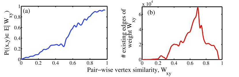
Figure 2: (a) Conditional probability of edge existence between authors with a given similarity $W_{xy}$ between their profiles; (b) actual number of edges with a given edge weight in the network.

Plot shown in Figure 2(a) confirms that our similarity measure is indeed proportional to the conditional probability of edge existence. We also observe the number of edges in a network having a particular edge weight $W_{xy}$ in Figure 2(b). Most of the edges are in the range $0.55-0.75$, indicating that this is the most common profile similarity range among pair-wise authors. Very few edges exist in the range $0-0.3$, which indicates that collaboration between authors with very dissimilar profiles is quite rare. This value also seems quite low for the range $0.9-1.0$, which might be due to the fact that it is extremely rare to have authors with nearly similar profiles.

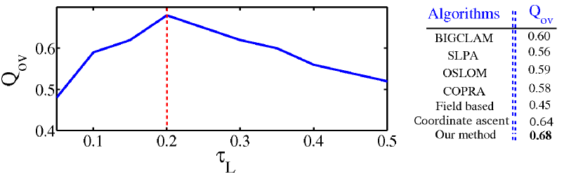
Figure 3: (Left) Change in overlapping modularity $Q_{ov}$ with the increase in $\tau_{L}$; (Right) comparison of the baseline algorithms with our method.

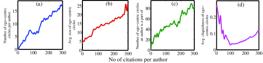
Figure 4: (Color online) Author-specific characterization of detected ego-centric circles. The following are plotted against the number of citations per author : (a) the number of circles centered around an author, (b) the average size of the circles centered around an author, (c) the number of ego-centric circles an author is a part of and (d) the average cliquishness of the circles centered around an author.

7 Evaluation of detected circles

In this section, we intend to evaluate the quality of the circles detected by our proposed methodology. Evaluation is especially important to judge the quality of the detected circles. We compare the circles detected by our model with that obtained from four other recent overlapping community detection algorithms, namely BIGCLAM [22], SLPA [20], OSLOM [13] and COPRA [10]. We also detect the circles using the coordinate ascent method (CA) [15, 16]. Since we intend to show that research field of the authors is not the proper information for creating the circles, we also compare our output with the circles obtained simply from research fields. For comparison, we use overlapping modularity $Q_{ov}$ [11] which is probably the most widely used measure for evaluating the goodness of a community structure without a ground-truth.

First, to show the change in $Q_{ov}$ with respect to the threshold $\tau_{L}$ as described in Section 4, we plot this quality function in Figure 3 by varying $\tau_{L}$ from 0.05-0.5. We observe that $Q_{ov}$ reaches maximum at $\tau_{L}=0.2$. Then for each competing algorithm, we measure the value of $Q_{ov}$ for each ego and take an average over all the egos present in our dataset. The table adjacent to Figure 3 shows that our method outperforms the traditional topology based community finding algorithms in detecting meaningful circles. Our method achieves $Q_{ov}$ of 0.68 which is 6.25% higher than coordinate ascent method, 13.33% higher than BIGCLAM, 15.25% higher than OSLOM, 17.24% higher than COPRA, and 21.42% higher than SLPA. We notice that research field based circles are the worst among the detected circles (see Section 9 for more discussion).

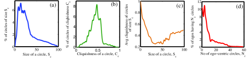
Figure 5: (Color online) Circle-specific characteristics of detected ego-centric circles: (a) distribution of the size of the ego-centric circles, (b) distribution of the cliquishness of the ego-centric circles, (c) average cliquishness of the circles having a particular size, and (d) percentage of egos surrounded by a particular number of ego-centric circles.

8 Analysis of Ego-Centric Circles

In this section, we intend to characterize the ego-centric circles obtained from our unsupervised model. In particular, we study the properties of the ego-centric circles at two levels of granularity: author-specific analysis and circle-specific analysis.

8.1 Author-specific Analysis

Here we study how the circles in the ego networks of the highly-cited authors differ from those of the low-cited authors. Figure 4(a) shows the number of ego-centric circles appearing in the ego network of each author. Note that in all of the experiments, we categorize authors into three groups: authors receiving more than 100 citations as highly-cited authors (proportion: 5.21%), authors receiving citations between 30-100 as medium-cited authors (proportion: 28.75%), and authors receiving less than 30 citations as low-cited authors (proportion: 66.04%). We notice a rise in the number of circles with the increase of citations. The possible reason could be that since the authors accumulating high citations tend to have high number of collaborators, the number of alters in their ego networks is also high, and thus more number of ego-centric circles are detected for the highly-cited authors.

In Figure 4(b), we plot the average size (measured in terms of the number of nodes) of the ego-centric circles for the authors in different citation range. Once again, the average size of the circles increases with the increase of citations per author. It essentially indicates that for the highly-cited egos, the alters are not only high in number but also form large cohesive groups.

Since each author is also an alter in her neighbors’ ego networks, she might be a part of multiple such ego-centric circles. Figure 4(c) shows the number of such ego-centric circles to which an author belongs to. This plot highly correlates with Figure 4(a), and shows that since highly-cited authors have more number of alters in their ego networks, each of them also belongs to multiple local circles of her neighbors’ ego networks.

Further, we measure the degree of cliquishness (the ratio of the number of existing edges in the circle and the maximum number of possible edges in the circle) of each ego-centric circle. For each ego, we measure the average cliquishness of her surrounding circles in the ego network. Figure 4(d) shows that the average value of cliquishness initially decreases with the increase of the number of citations per author, then it starts increasing. The reason could be that since both the number and the size of the ego-centric circles for low-cited authors are less, the maximum number of possible edges within a circle is also less, which in turn acts as the reason of high cliquishness for low-cited authors. In the middle citation zone, both the number and the average size of the circles are moderate. However, the number of edges that materialize within these circles is less as compared to the maximum number of possible edges, thus accounting for the sparseness of these circles. Therefore, the value of cliquishness of circles spawned by authors in the middle range of citations is comparatively low. However, the value of cliquishness starts increasing for the authors having citations more than 100. This signifies that for the highly-cited authors, despite the apparently large size of circles, the probability that an edge actually materializes in the real network tends to increase. This explains the formation of dense ego-centric cliques surrounding the ego in the high-citation range.

8.2 Circle-specific Analysis

Now we look into some of the characteristic features specific to an ego-centric circle. In Figure 5(a), we plot the percentage of ego-centric circles having a particular size $S_{c}$. It follows a Gaussian distribution at the beginning along with a heavy tail at the end. We observe that around 65.26% circles have sizes ranging between 4-30. However, the flat tail at the end shows that more than 15% circles have size greater than 50. Figure 5(b) shows the distribution of the cliquishness ($C_{c}$) of the ego-centric circles. Surprisingly, it again follows a Gaussian distribution with mean $\sim 0.44$ and variance $\sim 0.02$. We notice that around 59.28% circles have cliquishness values ranging between $[0.4,0.6]$ which is quite high. Further inspection reveals that low-degree egos are surrounded by small-size circles and therefore their cliquishness value is quite high. To get a clear idea of the relation between the size and the cliquishness of the ego-centric circles, we plot in Figure 5(c) the average cliquishness of the circles having a specific size. The value of cliquishness $C_{c}$ gradually decreases with the increase of the size $S_{c}$ till $S_{c}$=40, which is followed by a sharp increase. As mentioned earlier, the increase of cliquishness at the end once again emphasizes that the large-size circles centered around the highly-cited authors are relatively dense. Finally, we plot the percentage of egos surrounded by a specific number of circles in Figure 5(d). As expected, we observe that the plot has a declining trend from the very beginning, which once again highlights our previous observation that most of the low-cited authors have a low degree in the co-authorship network, and spawn only a few ego-centric circles. Since the co-authorship network is mostly dominated by low-degree authors, most of the egos are fringed by a small number of local circles.

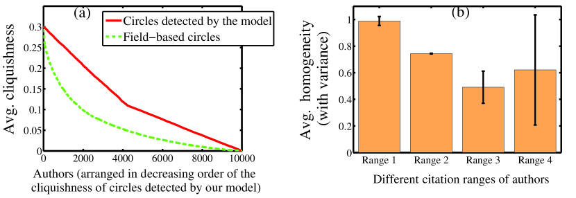
Figure 6: (Color online) (a) Comparison of cliquishness of area-based circles and the circles detected by our model, (b) average homogeneity of the ego-centric circles detected by our model for the authors categorized into four zones as per number of citations: Range 1 (>200), Range 2 (>100 & <=200), Range 3 (>30 & <=100) and Range 4 (<=30).

9 Interpretation of ego-centric circles

In co-authorship network, most intuitive ground-truth communities are often assumed to be different areas of research [7] in a particular domain. Therefore, one can interpret each ego-centric circle as a group of coauthors working in a specific research area. Since we know the major research area of each author in the dataset, for each ego we further group its coauthors based on only their major research area such that each circle corresponds to an area and constitutes coauthors working on this area. Then we measure the average cliquishness of the research field based circles for each author vis-a-vis that of the ego-centric circles detected by our model. Essentially, we intend to cross-validate our hypothesis that considering a single dimensional feature vector of an author such as the field information is not an appropriate way of encircling alters; rather each circle might represent individual dimension of cohesiveness among its constituent nodes as shown in Figure 1. In Figure 6(a), we plot the average cliquishness of field-based circles vis-a-vis that of the circles detected by the model surrounding each author. As expected, the cliquishness of the detected circles is significantly higher than that of the field-based circles. Therefore, we conclude that the field-based circles might not appropriately group highly cohesive nodes, rather the circles detected by our model seem to be more representative and meaningful.

We further mark each of the detected circles by that field which is also the major research area for most of its constituent coauthors. Then for each ego, we measure the fraction of circles belonging to each of the 24 fields. Therefore, each ego/author can now be represented by a vector of size 24 whose $i^{th}$ entry represents the fraction of ego-centric circles marked by field $i$. Figure 7 shows three heat maps corresponding to highly-cited, medium-cited and low-cited authors. For the sake of brevity, we only plot values for 1000 authors from each citation range although the results are similar for other authors. We observe that for highly-cited authors, ego-centric circles are mostly marked by few fields, which indicates that the highly-cited authors tend to collaborate with people from similar research area. If this is true, then the immediate question would be why the coauthors having same research interest are encircled into different groups by our model. Further inspection reveals that along with the field, each group also represents the time of collaboration. For instance, the ego network of Author 1 (one of the highly-cited authors) is shown in Figure 8(a). One group of her ego network encircles authors in Data Mining who have coauthored with her during 1997–2000. Another such group constitutes authors from Machine Learning, who have collaborated with her during 2000–2003. Therefore, the field of research and the time of collaboration act as two major dimensions in this case.

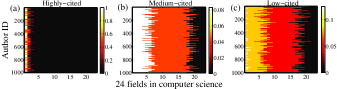
Figure 7: (Color online) Heat maps representing the fraction of ego-centric circles marked by each of the 24 fields for highly-cited, medium-cited and low-cited authors. For each author, the elements in the horizontal axis are sorted in descending order.

Next for the medium-cited authors, the heat map in Figure 7(b) shows that the distribution of circles into different fields seems to be much more uniform as compared to Figure 7(a). The example shown in Figure 8(b) also corroborates with the hypothesis that with the decrease of citations, the ego-centric circles tend to become even more complicated to be interpreted distinctly. From Figure 8(b), we notice that the time duration of collaboration corresponding to the circles are overlapping and, therefore, it is very hard to distinguish these circles. The result is even more cluttered for low-cited authors as shown in Figures 7(c) and 8(c). These results thus lead to a general conclusion that the highly-cited authors seem to coauthor with a group of people having a specific research interest in a particular time period and then move to another such group of coauthors; whereas this tendency is not so prominent for medium- and low-cited authors. However, we posit that there might be other dimensions (such as the name of the Institute where the author belongs to) that might help us interpret these circles more clearly.

Homogeneity of ego-centric circles. We define a field-based homogeneity for ego-centric circles to verify if, in most cases, authors from the same field tend to form communities and whether the circles spawned by our unsupervised approach are able to capture this tendency. Given a circle $C$, we define $F_{C,i}$ to be the fraction of authors in $C$ with major field $f_{i}$. One can easily infer that a uniform distribution $F_{C,i}$ implies that the circle is homogeneous with respect to the field of work while a skewed distribution (with majority of authors in one or two fields) characterizes a more field-specific circle. In particular, we define the homogeneity coefficient $H(C)$ for circle $C$ in terms of the entropy of the circle with respect to the distribution across different fields as in Equation 16. Greater the entropy, lesser is the homogeneity and vice versa.

$$H(C)=\frac{1}{1-\sum_{i=1}^{24}{F_{C,i}\log(F_{C,i})}}$$ (16)

Figure 6(b) captures the average homogeneity of circles in the ego-network of authors in four different citation ranges. We note that the homogeneity is highest for the authors with very high citation ranges $(>200)$ and has low variance, indicating that highly-cited authors tend to spawn circles that have alters in very similar fields, whereas authors with medium citations $(30-100)$ spawn more diverse circles. The authors with low citations $(\leq 30)$ exhibit higher degree of homogeneity than those in the medium range, but this may be attributed to the fact that they spawn very small-sized circles.

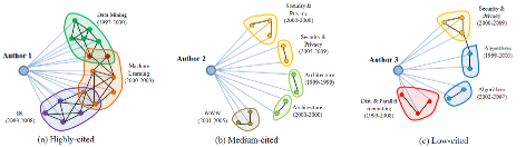
Figure 8: (Color online) Examples of ego-networks from three citation zones. Individual nodes have different colors corresponding to different areas of research. If the color of all the nodes in a circle is same as the color of the circle, the value of homogeneity is 1. Time period $(t_{i}-t_{j})$ associated with each circle indicates that the ego has written a paper first (last) time with anyone of its constituent coauthors at year $t_{i}$ ($t_{j}$).

10 Task based evaluation

We further evaluate the quality of the circles through a task based evaluation framework – the task of collaboration prediction. We choose two supervised learning models: linear regression (LR) [4] and supervised random walks (SRW) [4]. Then we demonstrate that inclusion of the ego-centric circles detected by our model as a feature in the feature set would eventually enhance the performance of this model with respect to the one in which the circle information is missing.

10.1 Problem Definition

For our problem, we assume a temporal graph $G_{T}=(V_{T},E_{T})$ where $V_{T}$ represents a set of nodes such that each node $u_{t}\in V_{T}$ is associated with a time stamp $t$ indicating its first appearance in $G_{T}$, and each edge $e_{t_{i},t_{j}}=(u_{t_{i}},v_{t_{j}})$ connects two nodes $u_{t_{i}}$ and $v_{t_{j}}$ (such that $u_{t_{i}}$,$v_{t_{j}}\in V_{T}$ and $t_{i}<=t_{j}$). Each node $u_{t}$ is also associated with a feature vector $f_{u_{t}}$ at time stamp $t$, whose entires might change over time. Now, given a longitudinal snapshot of the graph $G_{T}$ from the beginning till time $T^{{}^{\prime}}$, say $G_{T^{{}^{\prime}}}=(V_{T^{{}^{\prime}}},E_{T^{{}^{\prime}}})$, the collaboration prediction problem aims at predicting the collaborations which are going to appear among the vertices in $V_{T^{{}^{\prime}}}$ within $\Delta t$ time period after $T^{{}^{\prime}}$.

This task is very challenging due to extreme sparsity of real networks where each node is connected to only a very small fraction of all other nodes in the network (the presence of high proportion of negative evidences in the dataset).

10.2 Feature Set

We use a set of node- and edge-level features for the learning models. The following set of node-level features (denoted by $N$) are used. Each feature is normalized by the maximum value of the corresponding feature so that the values range between 0 to 1.
$\bullet$ Normalized number of citations received by an author
$\bullet$ Normalized h-index of an author
$\bullet$ Normalized number of coauthors of an author
$\bullet$ Fraction of papers by an author in each of the 24 fields
$\bullet$ Normalized number of papers written by an author
$\bullet$ Fraction of papers published by an author in each of the five decades (between 1960-2009)

Further, given an edge $e=(x,y)$ in the co-authorship network, we additionally use the following edge-level features (denoted by $E$). Each feature is appropriately normalized to a value between 0 and 1.
$\bullet$ Fraction of papers coauthored by $x$ and $y$ in each of the five decades
$\bullet$ Normalized number of common coauthors of $x$ and $y$
$\bullet$ Fraction of papers authored by $x$ in the major field of $y$
$\bullet$ Fraction of papers authored by $y$ in the major field of $x$

We refer to the combined set of both node- and edge-level features by $NE$. We provide this set $NE$ of node and edge attributes as an input to the learning model which then takes care of determining how to combine them with the network structure to make predictions [4]. Note that if we take the dataset till $t$ for training the model, all the features mentioned above will be calculated based on the statistics of each vertex till $t$ in order to avoid information leakage.

Table 1: Comparison of BIGCLAM (BIG), coordinate ascent method (CA) [15, 16] and our model (CIRC) after including their detected circle information into the feature set of Linear Regression (LR) and Supervised Random Walks (SRW) frameworks across three time periods and different feature sets (N: node-level, E: edge-level, NE: node- and edge-level, NEB: adding the binary circle information to NE, NEBC: adding the numerical circle information to NEB).

Time period	Area Under the ROC Curve (AUC)
	Linear Regression (LR)									Supervised Random Walks (SRW)
	N	E	NE	NEB			NEBC			N	E	NE	NEB			NEBC
				BIG	CA	CIRC	BIG	CA	CIRC				BIG	CA	CIRC	BIG	CA	CIRC
1996-1999	0.5872	0.5914	0.6451	0.6569	0.6689	0.6791	0.6989	0.7195	0.7235	0.6332	0.6478	0.7659	0.7908	0.7895	0.8275	0.7971	0.8296	0.8303
2001-2004	0.5890	0.5907	0.6528	0.6529	0.6437	0.6659	0.6845	0.7011	0.7012	0.6419	0.6514	0.7591	0.8067	0.8035	0.8249	0.8098	0.8149	0.8356
2006-2009	0.5916	0.5891	0.6436	0.6439	0.6510	0.6509	0.6905	0.7001	0.7198	0.6360	0.6608	0.7609	0.8001	0.8101	0.8295	0.8111	0.8279	0.8321
Average	0.5893	0.5904	0.6472	0.6512	0.6545	0.6653	0.6913	0.7069	0.7148	0.6370	0.6533	0.7620	0.7992	0.8101	0.8273	0.8060	0.8279	0.8327

Time period	$Prec@20$
	Linear Regression (LR)									Supervised Random Walks (SRW)
	N	E	NE	NEB			NEBC			N	E	NE	NEB			NEBC
				BIG	CA	CIRC	BIG	CA	CIRC				BIG	CA	CIRC	BIG	CA	CIRC
1996-1999	0.137	0.124	0.152	0.155	0.161	0.158	0.164	0.173	0.177	0.165	0.172	0.201	0.205	0.209	0.210	0.207	0.215	0.223
2001-2004	0.141	0.143	0.156	0.162	0.159	0.169	0.175	0.175	0.185	0.158	0.163	0.198	0.200	0.210	0.209	0.215	0.220	0.225
2006-2009	0.147	0.142	0.161	0.162	0.165	0.171	0.179	0.178	0.189	0.161	0.169	0.199	0.208	0.209	0.212	0.211	0.217	0.224
Average	0.142	0.136	0.156	0.160	0.162	0.166	0.173	0.175	0.184	0.161	0.168	0.199	0.204	0.209	0.210	0.211	0.217	0.224

10.3 Evaluation Methodology

In order to demonstrate that predictions are robust irrespective of the time stamp considered for dividing the dataset into training and test sets, we run the competing models in three different time periods: (i) the dataset till 1995 is considered for training and the accuracies of the models are measured by comparing the new edges formed between 1996-1999, (ii) similarly, the dataset till 2000 for training and 2001-2004 for checking the accuracy, and (iii) the dataset till 2005 for training and 2006-2009 for checking the accuracy.

In each time stamp, we evaluate the methods on the test set, considering two performance metrics: the Area under the ROC curve ($AUC$) and the Precision at Top 20 ($Prec@20$), i.e., for each node $s$, what fraction of top 20 nodes suggested by each model actually receive links from $s$ later. This measure is particularly appropriate in the context of link-recommendation where we present a user with a set of suggested coauthors and aim that most of them are correct.

10.4 Performance Evaluation

We compare the predictive performance of two learning models including the circle information in three different time periods as mentioned in Section 10.3. We iterate each of these collaboration prediction models using different sets of features: (i) only node-level features (Model: N), (ii) only edge-level features (Model: E), (iii) both node and edge level features (Model: NE), (iv) besides node and edge level features, including a binary feature $B$ that checks whether a pair of nodes $(x,y)$ belong to at least one common ego-centric circle or not (Model: NEB), and (v) besides node-level and edge-level features and the binary circle information, including a numeric feature $C$ indicating the number of common circles a pair of nodes $(x,y)$ is a part of (Model: NEBC). The circles are detected by our model, the coordinate ascent method (CA) [15, 16] and BIGCLAM separately.

Table 1 shows the performance of these two prediction models with different feature sets. We notice that edge features are more effective than node features, and the performance improves incrementally after combining different features together. A general observation is that inclusion of circle information in the feature set improves the performance of both the prediction models irrespective of the time periods. For instance, it improves the performance by $9.87\%$ and $15.25\%$ on average in terms of $AUC$ and $Prec@20$ respectively compared to the case, where the circle information is not present ($NE$).

We further observe that the inclusion of circle information detected by our model significantly outperforms the case where the circles are obtained by BIGCLAM and CA in each time stamp. Including the binary circle information ($NEB$) from our model achieves an average AUC improvement of 2.16% and 3.51% respectively for LR and SRW models (similarly, in terms of $Prec@20$, the improvement is 3.75% and 2.94% respectively for LR and SRW models) compared to BIGCLAM (CA).

Further, including the count of common circles for a node pair ($NEBC$) in the feature set leads both LR and SRW to achieve even better performance. We observe an average AUC improvement of 3.41% (1.11%) and 3.31% (0.57%) respectively for LR and SRW models using our circle information as compared to that obtained from BIGCLAM (CA) (similarly, in terms of $Prec@20$, the improvement is 6.35% (5.14%) and 6.16% (3.22%) respectively for LR and SRW models).

11 Conclusions and Future Work

Circles allow us to organize the overwhelming volumes of data generated by an author’s personal academic network. In this work, we proposed a simple yet effective method of detecting ego-centric circles in co-authorship networks. However, the proposed method is applicable to any general ego network given a suitable set of features. Our model is unsupervised and combines node attributes and node similarities to identify circles that resemble communities in real networks. Experiments with four state-of-the-art overlapping community detection algorithms showed that our method outperformed these baseline algorithms. Further, a task based evaluation achieved a superior performance after inclusion of the circle information detected by our model.

In future, we would like to develop a semi-supervised version of our algorithm that makes use of manually labeled data. Although most authors may not want to label the circles manually, it would be highly desirable to make use of the information from those few who do. Additionally, we would also like to apply the proposed method on the other datasets.

12 Acknowledgments

The first author is financially supported by Google India PhD fellowship.

References

- [1] A. Abbasi, K. S. K. Chung, and L. Hossain. Egocentric analysis of coauthorship network structure, position and performance. Inf. Process. Manage., 48(4):671–679, July 2012.
- [2] A. Abbasi, R. T. Wigand, and L. Hossain. Measuring social capital through network analysis and its influence on individual performance. Libr Inform Sci Res, 36(1):66 – 73, 2014.
- [3] E. M. Airoldi, D. M. Blei, S. E. Fienberg, and E. P. Xing. Mixed membership stochastic blockmodels. J. Mach. Learn. Res., 9:1981–2014, June 2008.
- [4] L. Backstrom and J. Leskovec. Supervised random walks: predicting and recommending links in social networks. In WSDM, pages 635–644, 2011.
- [5] R. Balasubramanyan and W. W. Cohen. Block-lda: Jointly modeling entity-annotated text and entity-entity links. In SDM, pages 450–461, 2011.
- [6] K. Börner, L. Dall’Asta, W. Ke, and A. Vespignani. Studying the emerging global brain: Analyzing and visualizing the impact of co-authorship teams: Research articles. Complex., 10(4):57–67, Mar. 2005.
- [7] T. Chakraborty, S. Sikdar, N. Ganguly, and A. Mukherjee. Citation interactions among computer science fields: a quantitative route to the rise and fall of scientific research. SNAM, 4(1), 2014.
- [8] J. P. Eaton, J. C. Ward, A. Kumar, and P. H. Reingen. Social-structural foundations of publication productivity in the Journal of Consumer Research. J Consum Res, 11(10):199–210, 2002.
- [9] S. Fortunato. Community detection in graphs. Physics Reports, 486(3-5):75 – 174, 2010.
- [10] S. Gregory. Finding overlapping communities in networks by label propagation. New Journal of Physics, 12(10):103018, 2010.
- [11] K. C. H. Shen, X. Cheng and M. B. Hu. Detect overlapping and hierarchical community structure in networks. Physica A, 388(8):1706–1712, 2009.
- [12] D. Jurafsky and J. H. Martin. Speech and Language Processing: An Introduction to Natural Language Processing, Computational Linguistics, and Speech Recognition. Prentice Hall PTR, USA, 2000.
- [13] A. Lancichinetti, F. Radicchi, J. J. Ramasco, and S. Fortunato. Finding statistically significant communities in networks. PLoS ONE, 6(4):e18961, 2011.
- [14] J. Liu and T. Liu. Detecting community structure in complex networks using simulated annealing with -means algorithms. Physica A, 389(11):2300–2309, 2010.
- [15] J. J. McAuley and J. Leskovec. Learning to discover social circles in ego networks. In NIPS, pages 548–556, 2012.
- [16] J. J. McAuley and J. Leskovec. Discovering social circles in ego networks. TKDD, 8(1):4, 2014.
- [17] C. McCarty, J. Jawitz, A. Hopkins, and A. Goldman. Predicting author h-index using characteristics of the co-author network. Scientometrics, 96(2):467–483, 2013.
- [18] A. Mislove, B. Viswanath, P. K. Gummadi, and P. Druschel. You are who you know: inferring user profiles in online social networks. In WSDM, pages 251–260, 2010.
- [19] M. E. J. Newman and M. Girvan. Finding and evaluating community structure in networks. Phys. Rev. E, 69(026113), 2004.
- [20] J. Xie and B. K. Szymanski. Towards linear time overlapping community detection in social networks. In PAKDD, pages 25–36, 2012.
- [21] E. Yan and Y. Ding. Applying centrality measures to impact analysis: A coauthorship network analysis. JASIST, 60(10):2107–2118, Oct. 2009.
- [22] J. Yang and J. Leskovec. Overlapping community detection at scale: A nonnegative matrix factorization approach. In WSDM, pages 587–596, New York, USA, 2013. ACM.