Large System Analysis of Cognitive Radio Network via Partially-Projected Regularized Zero-Forcing Precoding

Abstract

In this paper, we consider a cognitive radio (CR) network in which a secondary multiantenna base station (BS) attempts to communicate with multiple secondary users (SUs) using the radio frequency spectrum that is originally allocated to multiple primary users (PUs). Here, we employ partially-projected regularized zero-forcing (PP-RZF) precoding to control the amount of interference at the PUs and to minimize inter-SUs interference. The PP-RZF precoding partially projects the channels of the SUs into the null space of the channels from the secondary BS to the PUs. The regularization parameter and the projection control parameter are used to balance the transmissions to the PUs and the SUs. However, the search for the optimal parameters, which can maximize the ergodic sum-rate of the CR network, is a demanding process because it involves Monte-Carlo averaging. Then, we derive a deterministic expression for the ergodic sum-rate achieved by the PP-RZF precoding using recent advancements in large dimensional random matrix theory. The deterministic equivalent enables us to efficiently determine the two critical parameters in the PP-RZF precoding because no Monte-Carlo averaging is required. Several insights are also obtained through the analysis.

I Introduction

The radio frequency spectrum is a valuable but congested natural resource because it is shared by an increasing number of users. Cognitive radio (CR) [1, 2, 3, 4] is viewed as an effective means to improve the utilization of the radio frequency spectrum by introducing dynamic spectrum access technology. Such technology allows secondary users (SUs, also known as CR users) to access the radio spectrum originally allocated to primary users (PUs). In the CR literature, two cognitive spectrum access models have been widely adopted [4]: 1) the opportunistic spectrum access model and 2) the concurrent spectrum access model. In the opportunistic spectrum access model, SUs carry out spectrum sensing to detect spectrum holes and reconfigure their transmission to operate only in the identified holes [1, 5]. Meanwhile, in the concurrent spectrum access model, SUs transmit simultaneously with PUs as long as interference to PUs is limited [6, 7].

In this paper, we focus on the concurrent spectrum access model particularly when the secondary base station (BS) is equipped with multiple antennas. A desirable condition in the concurrent spectrum access model is for SUs to maximize their own performance while minimizing the interference caused to the PUs. Several transmit schemes have been studied to balance the transmissions to the SUs and the PUs [8, 9, 10, 11, 12]. In [8], a transmit algorithm has been proposed based on the singular value decomposition of the secondary channel after the projection into the null space of the channel from the secondary BS to the PUs. A spectrum sharing scheme has been designed for a large number of SUs [9], in which the SUs are pre-selected so that their channels are nearly orthogonal to the channels of the PUs. Doing so ensures that the SUs cause the lowest interference to the PUs.

In multi-antenna and multiuser downlink systems, a common technique to mitigate the multiuser interference is a zero-forcing (ZF) precoding [13, 14, 15, 16], which is computationally more efficient than its non-linear alternatives. However, the achievable rates of the ZF precoding are severely compromised when the channel matrix is ill conditioned. Then, regularized ZF (RZF) precoding [17, 18] is proposed to mitigate the ill-conditioned problem by employing a regularization parameter in the channel inversion. The regularization parameter can control the amount of introduced interference. Several applications based on the RZF framework have been developed, such as transmitter designs for non-CR broadcast systems [19, 20, 21, 22], security systems [23, 24], and multi-cell cooperative systems [25, 26, 27, 28].

While directly applying RZF to CR networks, the secondary BS can only control the interference in inter-SUs. A partially-projected RZF (PP-RZF) precoding has been proposed [10, 11], which limits the interference from the SUs to the PUs by combining the RZF [17, 18] with the channel projection idea [8]. The PP-RZF precoding follows the classical RZF technique, although the former is based on the partially-projected channel, which is obtained by partially projecting the channel matrix into the null space of the channel from the secondary BS to the PUs. The amount of interference to the PUs decreases with increasing amounts of projection into the null space of the PUs, which can be achieved by tuning the projection control parameter. However, the search for the optimal regularization parameter and projection control parameter is a demanding process because it involves Monte-Carlo averaging. Therefore, a deterministic (or large-system) approximation of the signal-to-interference-plus-noise ratio (SINR) for the PP-RZF scheme has been derived [10, 11]. Unfortunately, only the CR channel with a single PU has been studied and the scenario where multiple PUs are present remains unsolved [10].

To apply the PP-RZF precoding scheme in a CR network with multiple PUs, a new analytical technique that deals with a multi-dimensional random projection matrix, which is generated by partially projecting the channel matrix into the null spaces of multiple PUs, is required. This paper aims to address the above mentioned challenge by providing analytical results in a more general setting than that in [10, 11]. Specifically, we focus on a downlink multiuser CR network (Fig. 1), which consists of a secondary BS with multiple antennas, SUs, and PUs as well as different channel gains. Our main contributions are summarized below.

• We derive deterministic equivalents for the SINR and the ergodic sum-rate achieved by the PP-RZF precoding under the general CR network. Unlike previous works [10, 11], our model considers multiple PUs and allows different channel gains from the secondary BS to each user. Owing to recent advancements in large dimensional random matrix theory (RMT) with respect to complex combinations of different types of independent random matrices [29], we identify the large system distribution of the Stieltjes transform for a new class of random matrix. Therefore, our extension becomes non trivial and novel.

• In the PP-RZF precoding, the regularization parameter and the projection control parameter can regulate the amount of interference to the SUs and the PUs, but a wrong choice of parameters can considerably degrade the performance of the CR network. However, the search for the optimal parameters is a demanding process because Monte-Carlo averaging is required. We overcome the fundamental difficulty of applying PP-RZF precoding in the CR network. The deterministic equivalent for the ergodic sum-rate provides an efficient way of finding the asymptotically optimal regularization parameter and the asymptotically optimal projection control parameter. Simulation results indicate good agreement with the optimum in terms of the ergodic sum-rate.

• We provide several useful observations on the condition that the regularization parameter and the projection control parameter can achieve the optimal sum-rate. We also reveal the relationship between the parameters and the signal-to-noise ratio (SNR).

Notations—We use uppercase and lowercase boldface letters to denote matrices and vectors, respectively. An $N\times N$ identity matrix is denoted by ${\bf{I}}_{N}$, an all-zero matrix by ${\bf 0}$, and an all-one matrix by ${\bf 1}$. The superscripts $(\cdot)^{H}$, $(\cdot)^{T}$, and $(\cdot)^{*}$ denote the conjugate transpose, transpose, and conjugate operations, respectively. ${\sf E}\{\cdot\}$ returns the expectation with respect to all random variables within the bracket, and $\log(\cdot)$ is the natural logarithm. We use $[{\bf A}]_{kl}$, $[{\bf A}]_{l,k}$, or $A_{kl}$ to denote the ($k$,$l$)-th entry of the matrix $\bf A$, and $a_{k}$ denotes the $k$-th entry of the column vector $\bf{a}$. The operators $(\cdot)^{\frac{1}{2}}$, $(\cdot)^{-1}$, ${{\sf tr}}(\cdot)$, and $\det(\cdot)$ represent the matrix principal square root, inverse, trace, and determinant, respectively, $\|\cdot\|$ represents the Euclidean norm of an input vector or the spectral norm of an input matrix, and ${\sf diag}(\bf{x})$ denotes a diagonal matrix with $\bf{x}$ along its main diagonal. The notation “$\xrightarrow{a.s.}$” denotes the almost sure (a.s.) convergence.

II System Model and Problem Formulation

II-A System Model

Figure 1: A downlink multiuser cognitive radio network.

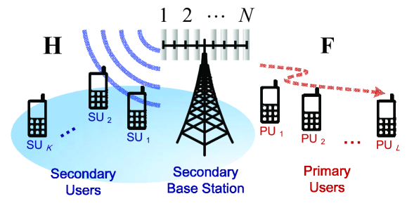
As illustrated in Fig. 1, we consider a downlink multiuser CR network that consists of a secondary BS with $N$ antennas (labeled as ${\sf BS}$). The ${\sf BS}$ simultaneously transmits $K$ independent messages to $K$ single antenna SUs (labeled as ${\sf SU}_{1},\dots,{\sf SU}_{K}$). We assume that all the SUs share the same spectrum with $L$ single antenna PUs (labeled as ${\sf PU}_{1},\dots,{\sf PU}_{L}$). Let ${\bf h}_{k}^{H}\in{\mathbb{C}}^{1\times N}$ be the fading channel vector between ${\sf BS}$ and ${\sf SU}_{k}$, ${\bf f}_{l}^{H}\in{\mathbb{C}}^{1\times N}$ be the fading channel vector between ${\sf BS}$ and ${\sf PU}_{l}$, and ${\bf g}_{k}\in{\mathbb{C}}^{N\times 1}$ be the precoding vector of ${\sf SU}_{k}$. The received signal at ${\sf SU}_{k}$ can therefore be expressed as

$$y_{k}={\bf h}_{k}^{H}{\bf g}_{k}s_{k}+\sum_{j=1,j\neq k}^{K}{\bf h}_{k}^{H}{\bf g}_{j}s_{j}+z_{k},$$ (1)

where $s_{k}$ is the data symbol of ${\sf SU}_{k}$, $s_{j}$’s are independent and identically distributed (i.i.d.) data symbols with zero mean and unit variance, respectively, and $z_{k}$ is the additive Gaussian noise with zero mean and variance of $\sigma^{2}$. For ease of exposition, we define ${\bf H}\triangleq\left[{\bf h}_{1},\dots,{\bf h}_{K}\right]^{H}\in{\mathbb{C}}^{K\times N}$, ${\bf F}\triangleq\left[{\bf f}_{1},\dots,{\bf f}_{L}\right]^{H}\in{\mathbb{C}}^{L\times N}$, ${\bf G}\triangleq\left[{\bf g}_{1},\dots,{\bf g}_{K}\right]\in{\mathbb{C}}^{N\times K}$, ${\bf y}\triangleq[{y_{1}},\dots,{y_{K}}]^{T}\in{\mathbb{C}}^{K}$, ${\bf s}\triangleq\left[{s_{1}},\dots,{s_{K}}\right]^{T}\in{\mathbb{C}}^{K}$, and ${\bf z}\triangleq\left[{z_{1}},\dots,{z_{K}}\right]^{T}\in{\mathbb{C}}^{K}$. The received signal of all the SUs in vector form is given by

$${\bf y}={\bf H}{\bf G}{\bf s}+{\bf z}.$$ (2)

We also assume that ${\sf BS}$ satisfies the average total transmit power constraint

$${\sf E}\left\{{\sf tr}\left({\bf G}{\bf G}^{H}\right)\right\}\leq{NP_{T}},$$ (3)

where $P_{T}>0$ is the parameter that determines the power budget of ${\sf BS}$. Notably, if we consider the instantaneous transmit power constraint, i.e., ${\sf tr}({\bf G}{\bf G}^{H})\leq{NP_{T}}$, we can obtain the same constraint in a large-system regime, as shown in Appendix B-III.

The peak received interference power constraint or the average received interference power constraint is used to protect the PUs. Given that the latter is more flexible for dynamically allocating transmission powers over different fading states than the former [30, 31], we employ the average received interference power constraint and consider two cases: Case I—the average received interference power constraint at each PU and Case II—the total average received interference power constraint at all PUs. These cases are respectively given by

$$\mbox{Case I (Per PU power constraint):~{}~{}~{}~{}}{\sf E}\left\{{\bf f}_{l}^{H}{\bf G}{\bf G}^{H}{\bf f}_{l}\right\}\leq P_{l},\mbox{~{}~{}for}~{}~{}l=1,\ldots,L,$$ (4a)

$$\mbox{Case II (Sum power constraint):~{}~{}~{}~{}}{\sf E}\left\{{\sf tr}\left({\bf F}{\bf G}{\bf G}^{H}{\bf F}^{H}\right)\right\}\leq P_{\rm all},$$ (4b)

where $P_{l}>0$ denotes the interference power threshold of ${\sf PU}_{l}$, and $P_{\rm all}>0$ represents the total interference power threshold of all PUs. We then set $P_{l}=\theta_{l}P_{T}$ and $P_{\rm all}=\theta_{\rm all}P_{T}$ with $\theta_{l},\theta_{\rm all}$ being positive scalar parameters to make a connection with the transmit power. Although we only consider equal power allocation for simplicity in this paper, our framework can be easily extended to arbitrary power allocation by replacing ${\bf G}$ with ${\bf G}{\bf P}^{\frac{1}{2}}$, where ${\bf P}={\sf diag}(p_{1},\ldots,p_{K})$ with $p_{k}\geq 0$ being the signal power of ${\sf SU}_{k}$ (see [21, 22] for a similar application).

Next, to incorporate path loss and other large-scale fading effects, we model the channel vectors by

$${\bf h}_{k}^{H} =\sqrt{r_{1,k}}\,{\tilde{{\bf h}}}_{k}^{H}\mbox{~{}~{}and}~{}~{}{\bf f}_{l}^{H}=\sqrt{r_{2,l}}\,{\tilde{{\bf f}}}_{l}^{H},$$ (5)

where ${\tilde{{\bf h}}}_{k}^{H}$ and ${\tilde{{\bf f}}}_{l}^{H}$ are the small-scale (or fast) fading vectors, and $r_{1,k}$ and $r_{2,l}$ denote the large-scale fading coefficients (or channel path gains), including the geometric attenuation and shadow effect. Using the above notations, the concerned channel matrices can be rewritten as

$${\bf H} ={\bf R}_{1}^{\frac{1}{2}}{\tilde{{\bf H}}}\mbox{~{}~{}and}~{}~{}{\bf F}={\bf R}_{2}^{\frac{1}{2}}{\tilde{{\bf F}}},$$ (6)

where ${\tilde{{\bf H}}}\equiv[\frac{1}{\sqrt{N}}\tilde{h}_{ij}]\in{\mathbb{C}}^{K\times N}$ and ${\tilde{{\bf F}}}\equiv[\frac{1}{\sqrt{N}}\tilde{f}_{ij}]\in{\mathbb{C}}^{L\times N}$ consist of the random components of the channel in which $\tilde{h}_{ij}$’s and $\tilde{f}_{ij}$’s are i.i.d. complex random variables with zero mean and unit variance, respectively, and ${\bf R}_{1}\in{\mathbb{C}}^{K\times K}$ and ${\bf R}_{2}\in{\mathbb{C}}^{L\times L}$ are diagonal matrices whose diagonal elements are given by $[{\bf R}_{1}]_{kk}=r_{1,k}$ and $[{\bf R}_{2}]_{ll}=r_{2,l}$, respectively. In line with [10, 11], we assume that ${\bf H}$ is perfectly known to ${\sf BS}$ in this paper. Since ${\sf BS}$ needs to predict the interference power in (4), we further assume that perfect knowledge of ${\bf F}$ is available at ${\sf BS}$ [32, 10, 11]. To acquire perfect channel state information (CSI) for ${\bf H}$ and ${\bf F}$, transmission protocols need to incorporate certain cooperation among the PUs, the SUs, and ${\sf BS}$ [32]. Further research can focus on the case with imperfect CSI or estimation of channel [33, 34].

In the downlink CR network (2), we consider the RZF precoding because this precoding’s relatively low complexity compared with dirty paper coding [17, 18, 21, 27]. However, a direct application of the conventional RZF to the secondary BS will result in a very inefficient transmission because a large power back-off at the secondary BS is required to satisfy the interference power constraint (4). Therefore, following [10, 11], we adopt the RZF precoding based on the partially-projected channel matrix

$$\check{{\bf H}}={\bf H}({\bf I}_{N}-\beta{\bf W}^{H}{\bf W}),$$ (7)

where ${\bf W}\triangleq({\bf F}{\bf F}^{H})^{-\frac{1}{2}}{\bf F}\in{\mathbb{C}}^{L\times N}$, and $\beta\in[0,1]$ is the projection control parameter. Note that the projected channel matrix $\check{{\bf H}}$ is obtained by partially projecting ${\bf H}$ into the null space of ${\bf F}$. Specifically, the RZF precoding matrix is given by

$${\bf G}=\xi\left(\check{{\bf H}}^{H}\check{{\bf H}}+\alpha{\bf I}_{N}\right)^{-1}\check{{\bf H}}^{H},$$ (8)

where $\xi$ is a normalization parameter that fulfills the BS transmit power constraint (3) and the interference power constraint (4), and $\alpha>0$ represents the regularization parameter. We refer to this precoding as PP-RZF precoding.

Before setting each of the parameters in (8), two special cases of the PP-RZF precoding are considered first. On the one hand, if $\beta=0$ then ${\bf G}$ degrades to the conventional RZF precoding. On the other hand, if $\beta=1$ then $\check{{\bf H}}$ is completely orthogonal to ${\bf F}$ and we have ${\bf F}\check{{\bf H}}^{H}={\bf 0}$, i.e., no interference signal from the secondary BS will leak to the PUs. Therefore, the interference power constraint (4) is naturally guaranteed. Furthermore, the amount of the interference to the PUs decreases as the projection control parameter increases.

Now we return to the setting of the normalization parameter in (8). Considering Case I, from (3) and (4a), we have

$$\xi^{2}\leq \xi_{0}^{2}\triangleq\frac{P_{T}}{{\sf E}\left\{\frac{1}{N}{\sf tr}\left(\left(\check{{\bf H}}^{H}\check{{\bf H}}+\alpha{\bf I}_{N}\right)^{-1}\check{{\bf H}}^{H}\check{{\bf H}}\left(\check{{\bf H}}^{H}\check{{\bf H}}+\alpha{\bf I}_{N}\right)^{-1}\right)\right\}},$$ (9a)

$$\xi^{2}\leq \xi_{l}^{2}\triangleq\frac{\theta_{l}P_{T}}{{\sf E}\left\{{\bf f}_{l}^{H}\left(\check{{\bf H}}^{H}\check{{\bf H}}+\alpha{\bf I}_{N}\right)^{-1}\check{{\bf H}}^{H}\check{{\bf H}}\left(\check{{\bf H}}^{H}\check{{\bf H}}+\alpha{\bf I}_{N}\right)^{-1}{\bf f}_{l}\right\}},\mbox{~{}~{}for}~{}l=1,\ldots,L.$$ (9b)

To satisfy (3) and (4a) simultaneously, we set $\xi^{2}=\min\{\xi_{0}^{2},\xi_{l}^{2},l=1,\ldots,L\}$. Then, the SINR of secondary user ${\sf SU}_{k}$ is given by

$$\gamma_{k} =\frac{\left|{\bf h}_{k}^{H}\left(\check{{\bf H}}^{H}\check{{\bf H}}+\alpha{\bf I}_{N}\right)^{-1}\check{{\bf h}}_{k}\right|^{2}}{{\bf h}_{k}^{H}\left(\check{{\bf H}}^{H}\check{{\bf H}}+\alpha{\bf I}_{N}\right)^{-1}\check{{\bf H}}_{[k]}^{H}\check{{\bf H}}_{[k]}\left(\check{{\bf H}}^{H}\check{{\bf H}}+\alpha{\bf I}_{N}\right)^{-1}{\bf h}_{k}+\frac{\sigma^{2}}{\xi^{2}}}$$

$$=\frac{\rho\left|{\bf h}_{k}^{H}\left(\check{{\bf H}}^{H}\check{{\bf H}}+\alpha{\bf I}_{N}\right)^{-1}\check{{\bf h}}_{k}\right|^{2}}{\rho{\bf h}_{k}^{H}\left(\check{{\bf H}}^{H}\check{{\bf H}}+\alpha{\bf I}_{N}\right)^{-1}\check{{\bf H}}_{[k]}^{H}\check{{\bf H}}_{[k]}\left(\check{{\bf H}}^{H}\check{{\bf H}}+\alpha{\bf I}_{N}\right)^{-1}{\bf h}_{k}+\nu},$$ (10)

where $\check{{\bf H}}_{[k]}\triangleq[\check{{\bf h}}_{1},\ldots,\check{{\bf h}}_{k-1},\check{{\bf h}}_{k+1},\ldots,\check{{\bf h}}_{K}]^{H}\in{\mathbb{C}}^{(K-1)\times N}$, $\check{{\bf h}}_{k}\triangleq({\bf I}_{N}-\beta{\bf W}^{H}{\bf W}){\bf h}_{k}$, $\rho\triangleq P_{T}/\sigma^{2}$, and

$$\nu\triangleq\frac{P_{T}}{\xi^{2}}=\max \bigg{\{}{\sf E}\left\{\frac{1}{N}{\sf tr}\left(\left(\check{{\bf H}}^{H}\check{{\bf H}}+\alpha{\bf I}_{N}\right)^{-1}\check{{\bf H}}^{H}\check{{\bf H}}\left(\check{{\bf H}}^{H}\check{{\bf H}}+\alpha{\bf I}_{N}\right)^{-1}\right)\right\},$$

$$~{}~{}~{}~{}\frac{1}{\theta_{l}}{\sf E}\left\{{\bf f}_{l}^{H}\left(\check{{\bf H}}^{H}\check{{\bf H}}+\alpha{\bf I}_{N}\right)^{-1}\check{{\bf H}}^{H}\check{{\bf H}}\left(\check{{\bf H}}^{H}\check{{\bf H}}+\alpha{\bf I}_{N}\right)^{-1}{\bf f}_{l}\right\},l=1,\ldots,L\bigg{\}}.$$ (11)

Here, the equality of (11) follows from (9). For Case II, we have

$$\nu=\max \bigg{\{}{\sf E}\left\{\frac{1}{N}{\sf tr}\left(\left(\check{{\bf H}}^{H}\check{{\bf H}}+\alpha{\bf I}_{N}\right)^{-1}\check{{\bf H}}^{H}\check{{\bf H}}\left(\check{{\bf H}}^{H}\check{{\bf H}}+\alpha{\bf I}_{N}\right)^{-1}\right)\right\},$$

$$~{}~{}~{}~{}\frac{1}{\theta_{\rm all}}{\sf E}\left\{{\sf tr}\left({\bf F}\left(\check{{\bf H}}^{H}\check{{\bf H}}+\alpha{\bf I}_{N}\right)^{-1}\check{{\bf H}}^{H}\check{{\bf H}}\left(\check{{\bf H}}^{H}\check{{\bf H}}+\alpha{\bf I}_{N}\right)^{-1}{\bf F}^{H}\right)\right\}\bigg{\}}.$$ (12)

Consequently, under the assumption of perfect CSI at both transmitter and receivers, the ergodic sum-rate of the CR network with Gaussian signaling can be defined as

$$R_{\rm{sum}}\triangleq\sum_{k=1}^{K}{\sf E}\left\{\log\left(1+\gamma_{k}\right)\right\}.$$ (13)

Note that $\gamma_{k}$ in the ergodic sum-rate is subject to the BS transmit power constraint in (3) and the interference power constraint (to the primary users) in (4).

II-B Problem Formulation

The SINR $\gamma_{k}$ in (II-A) is a function of the regularization parameter $\alpha$ and the projection control parameter $\beta$. In the literature, adopting incorrect regularization parameter would degrade performance significantly [18, 21, 27]. In light of the discussion in the previous subsection, one can realize that a proper projection control parameter can assist in decreasing the interference to the PUs. As a result, using the PP-RZF precoding effectively requires obtaining appropriate values of $\alpha$ and $\beta$ to optimize certain performance metrics. In this paper, we are interested in finding $(\alpha,\beta)$, which maximizes the ergodic sum-rate (13). Formally, we have

$$\left\{\alpha^{\rm opt},\beta^{\rm opt}\right\}=\operatornamewithlimits{arg\,max}_{\alpha>0,1\geq\beta\geq 0} ~{}R_{\rm{sum}}.$$ (14)

The above problem does not admit a simple closed-form solution and the solution must be computed via a two-dimensional line search. Monte-Carlo averaging over the channels is required to evaluate the ergodic sum-rate (13) for each choice of $\alpha$ and $\beta$, which, unfortunately, makes the overall computational complexity prohibitive. This drawback hinders the development of the PP-RZF precoding. To address this problem, we resort to an asymptotic expression of (13) in the large-system regime in the next section.

III Performance Analysis of Large Systems

This section presents the main results of the paper. First, we derive deterministic equivalents for the SINR $\gamma_{k}$ and the ergodic sum-rate $R_{\rm{sum}}$ in a large-system regime. Then, we identify the asymptotically optimal regularization parameter and the asymptotically optimal projection control parameter to achieve the optimal deterministic equivalent for the ergodic sum-rate.

III-A Deterministic Equivalents for the SINR and the Ergodic Sum-Rate

We present a deterministic equivalent for the SINR $\gamma_{k}$ by considering the large-system regime, where $N$, $K$, and $L$ approach infinity, whereas

$$c_{1}=\frac{N}{K}\mbox{~{}~{}and~{}~{}}c_{2}=\frac{L}{N}$$

are fixed ratios, such that $0<\lim\inf_{N}c_{1}\leq\lim\sup_{N}c_{1}<\infty,0<\lim\inf_{N}c_{2}\leq\lim\sup_{N}c_{2}\leq 1$. For brevity, we simply use ${\mathcal{N}}\rightarrow\infty$ to represent the quantity in such limit. In addition, we impose the assumptions below in our derivations.

Assumption 1

For the channel matrices ${\bf H}$ and ${\bf G}$ in (6), we have the following hypotheses:

• ${\tilde{{\bf H}}}=[\frac{1}{\sqrt{N}}\tilde{h}_{ij}]\in{\mathbb{C}}^{K\times N}$, where $\tilde{h}_{ij}$’s are i.i.d. standard Gaussian.

• ${\tilde{{\bf F}}}=[\frac{1}{\sqrt{N}}\tilde{f}_{ij}]\in{\mathbb{C}}^{L\times N}$, where $\tilde{f}_{ij}$’s have the same statistical properties as $\tilde{h}_{ij}$’s.

• ${\bf R}_{1}={\sf diag}(r_{1,1},\ldots,r_{1,K})\in{\mathbb{C}}^{K\times K}$ and ${\bf R}_{2}={\sf diag}(r_{2,1},\ldots,r_{2,L})\in{\mathbb{C}}^{L\times L}$ are diagonal matrices with uniformly bounded spectral norm with respect to $K$ and $L$, respectively.

Based on the definition of ${\bf W}$ in (7), ${\bf W}^{H}{\bf W}={\bf F}^{H}({\bf F}{\bf F}^{H})^{-1}{\bf F}={\tilde{{\bf F}}}^{H}({\tilde{{\bf F}}}{\tilde{{\bf F}}}^{H})^{-1}{\tilde{{\bf F}}}$ $={\tilde{{\bf W}}}^{H}{\tilde{{\bf W}}}$, where ${\tilde{{\bf W}}}\triangleq({\tilde{{\bf F}}}{\tilde{{\bf F}}}^{H})^{-\frac{1}{2}}{\tilde{{\bf F}}}$. Therefore, ${\tilde{{\bf W}}}$ is $L\leq N$ rows of an $N\times N$ Haar-distributed unitary random matrix [29, Definition 4.6]. The partially-projected channel matrix $\check{{\bf H}}$ is clearly composed of the product of two different types of independent random matrices. Owing to recent advancements in large dimensional RMT [29], we arrive at the following theorem, and the details are given in Appendix A.

Theorem 1

Under Assumption 1, in Case I (per PU power constraint), as ${\mathcal{N}}\rightarrow\infty$, we have $\gamma_{k}-\overline{\gamma}_{k}\xrightarrow{a.s.}0$, for $k=1,\dots,K$, where

$$\overline{\gamma}_{k} =\frac{\rho\overline{a}_{k}^{2}}{\rho\overline{b}_{k}+\overline{\nu}},$$ (15)

with

$$\overline{a}_{k} =\frac{r_{1,k}(t_{1}+t_{2}(1-\beta))}{\alpha+r_{1,k}(t_{1}+t_{2}(1-\beta)^{2})},$$ (16a)

$$\overline{b}_{k} =r_{1,k}\left(\frac{\left(1-\overline{a}_{k}\right)^{2}t_{1}}{1+e}+\frac{\left(1-(1-\beta)\overline{a}_{k}\right)^{2}(1-\beta)^{2}t_{2}}{1+(1-\beta)^{2}e}\right)\frac{\partial e}{\partial\alpha},$$ (16b)

$$\overline{\nu} =\max\bigg{\{}\left(\frac{t_{1}}{1+e}+\frac{(1-\beta)^{2}t_{2}}{1+(1-\beta)^{2}e}\right)\frac{\partial e}{\partial\alpha},\frac{r_{2,l}}{\theta_{l}c_{2}}\frac{(1-\beta)^{2}t_{2}}{1+(1-\beta)^{2}e}\frac{\partial e}{\partial\alpha},l=1,\ldots,L\bigg{\}},$$ (16c)

$$\frac{\partial e}{\partial\alpha} =\frac{\frac{1}{N}{\sf tr}{\bf R}_{1}\left(\alpha{\bf I}_{K}+\left(t_{1}+t_{2}(1-\beta)^{2}\right){\bf R}_{1}\right)^{-2}}{1-\left(\frac{t_{1}}{1+e}+\frac{(1-\beta)^{4}t_{2}}{1+(1-\beta)^{2}e}\right)\frac{1}{N}{\sf tr}\left({\bf R}_{1}\left(\alpha{\bf I}_{K}+\left(t_{1}+t_{2}(1-\beta)^{2}\right){\bf R}_{1}\right)^{-1}\right)^{2}},$$ (16d)

$$t_{1} =\frac{1-c_{2}}{1+e},~{}~{}~{}~{}~{}~{}~{}~{}t_{2}=\frac{c_{2}}{1+(1-\beta)^{2}e},$$ (16e)

and $e$ is given as the unique solution to the fixed point equation

$$e= \frac{1}{N}{\sf tr}{\bf R}_{1}\left(\alpha{\bf I}_{K}+\left(t_{1}+t_{2}(1-\beta)^{2}\right){\bf R}_{1}\right)^{-1}.$$ (17)

Meanwhile, in Case II (sum power constraint), all asymptotic expressions remain, except for $\overline{\nu}$, which should be changed to

$$\overline{\nu} =\max\bigg{\{}\left(\frac{t_{1}}{1+e}+\frac{(1-\beta)^{2}t_{2}}{1+(1-\beta)^{2}e}\right)\frac{\partial e}{\partial\alpha},\frac{{\sf tr}{\bf R}_{2}}{\theta_{\rm all}c_{2}}\frac{(1-\beta)^{2}t_{2}}{1+(1-\beta)^{2}e}\frac{\partial e}{\partial\alpha}\bigg{\}}.$$ (18)

$\blacksquare$

An intuitive application of Theorem 1 is that $\gamma_{k}$ can be approximated by its deterministic equivalent $\overline{\gamma}_{k}$, which can be determined based only on statistical channel knowledge, that is, ${\bf R}_{1}$, ${\bf R}_{2}$, and $\sigma^{2}$. Note that, according to the definition of the deterministic equivalent (see footnote 3), in the expression of the deterministic equivalent $\overline{\gamma}_{k}$, the parameters $N$, $K$, $L$, as well as the matrix dimensions of ${\bf R}_{1}$ and ${\bf R}_{2}$, are finite. Combining Theorem 1 with the continuous mapping theorem, we have $\log\left(1+\gamma_{k}\right)-\log\left(1+\overline{\gamma}_{k}\right)\xrightarrow{a.s.}0$. An approximation $\overline{R}_{\rm{sum}}$ of the ergodic sum-rate $R_{\rm{sum}}$ in (13) is obtained by replacing the instantaneous SINR $\gamma_{k}$ with its large system approximation $\overline{\gamma}_{k}$, that is,

$$\overline{R}_{\rm{sum}}=\sum_{k=1}^{K}\log\left(1+\overline{\gamma}_{k}\right).$$ (19)

Therefore, when ${\mathcal{N}}\rightarrow\infty,\frac{1}{K}\left(R_{\rm{sum}}-\overline{R}_{\rm{sum}}\right)\xrightarrow{a.s.}0$ holds true almost surely.

To facilitate our understanding of Theorem 1, we look at it from the two special cases as follows:

1. In Theorem 1, we introduce the two variables $t_{1}$ and $t_{2}$ to reflect the effects of the projection control parameter $\beta$. If $\beta=1$, from (16), then the deterministic equivalent $\overline{\gamma}_{k}$ does not depend on $t_{2}$. Substituting $\beta=1$ into (15) and letting ${\bf R}_{1}={\bf I}_{K}$, we have

   $$\overline{\gamma}_{k} =\frac{\rho\Big{(}c_{1}(1-c_{2})(1+\zeta(\mu,\eta,\alpha))^{2}-\zeta(\mu,\eta,\alpha)^{2}\Big{)}}{\rho+\Big{(}1+\zeta(\mu,\eta,\alpha)\Big{)}^{2}},$$ (20)

   where $\zeta(\mu,\eta,\alpha)\triangleq t_{1}/\alpha$, $\mu\triangleq 1-c_{2}$, and $\eta\triangleq 1/c_{1}$. Combining (16e) and (17), we obtain

   $$\zeta(\mu,\eta,\alpha)\triangleq\frac{t_{1}}{\alpha}=\frac{1}{2}\left(\frac{\mu-\eta}{\alpha}-1+\sqrt{\frac{(\mu-\eta)^{2}}{\alpha^{2}}+\frac{2(\mu+\eta)}{\alpha}+1}\,\right).$$ (21)

   Before providing an observation based on the above, we briefly review a well-known result from the large dimensional RMT. First, we consider the definition of ${\bf H}$ from (6). If ${\bf R}_{1}={\bf I}_{K}$, the entries of the $K\times N$ matrix ${\bf H}$ are zero mean i.i.d. with variance $1/N$. Following [29, Chapter 3], we see that as $N,\,K\rightarrow\infty$ with $N/K\rightarrow c_{1}$, ${\bf h}_{k}^{H}\left({\bf H}^{H}{\bf H}+\alpha{\bf I}_{N}\right)^{-1}{\bf h}_{k}$ converges almost surely to

   $$\int_{a}^{b}\frac{1}{\lambda+\alpha}f(\lambda)\,d\lambda,$$ (22)

   where

   $$f(\lambda)=\left(1-\eta\right)^{+}\delta(\lambda)+\frac{\sqrt{(\lambda-a)^{+}(b-\lambda)^{+}}}{2\pi\lambda}$$ (23)

   with $(x)^{+}\triangleq\max\{x,\,0\}$, $a\triangleq(1-\sqrt{\eta})^{2}$, and $b\triangleq(1+\sqrt{\eta})^{2}$. In fact, $f(u)$ is the limiting empirical distribution of the eigenvalues of ${\bf H}^{H}{\bf H}$ and is known as the Marčcenko-Pastur law [38]. The integral of (22) can be evaluated in closed form

   $$\frac{1}{2}\left(\frac{1-\eta}{\alpha}-1+\sqrt{\frac{(1-\eta)^{2}}{\alpha^{2}}+\frac{2(1+\eta)}{\alpha}+1}\,\right).$$ (24)

   Note that (21) is equal to (24) when $\mu$ is replaced with $1$, i.e., (24) is equal to $\zeta(1,\eta,\alpha)$. In fact, following the similar derivations of Theorem 1, we can show that (20) and the SINR of the conventional RZF precoding share the same formulation by replacing $\zeta(\mu,\eta,\alpha)$ in (20) with $\zeta(1,\eta,\alpha)$. Substituting the definitions of $c_{1},c_{2}$ into $\mu$ and $\eta$, we have $\mu-\eta=1-c_{2}-1/c_{1}=(N-(L+K))/N$. Comparing this value with $1-\eta=(N-K)/N$ in (24), we thus conclude that if $\beta=1$, the SINR of the PP-RZF precoding is similar to that of the conventional RZF precoding but with an increase in the number of active users from $K$ to $K+L$. Hence, the degrees of freedom of the PP-RZF precoding is reduced to $N-(K+L)$ because the additional $L$ degrees of freedom are used to suppress interference to the PUs.

2. For another extreme case with $\beta=0$ in Theorem 1, $t_{1}+t_{2}=\frac{1}{1+e}$. Letting ${\bf R}_{1}={\bf I}_{K}$, we obtain $\frac{1}{\alpha(1+e)}=\zeta(1,\eta,\alpha)$, such that

   $$\overline{\gamma}_{k} =\frac{\rho\Big{(}c_{1}(1+\zeta(1,\eta,\alpha))^{2}-\zeta(1,\eta,\alpha)^{2}\Big{)}}{\rho+\nu_{0}\Big{(}1+\zeta(1,\eta,\alpha)\Big{)}^{2}},$$ (25)

   where $\nu_{0}=\max\{1,r_{2,l}/\theta_{l},l=1,\ldots,L\}$ is for Case I and $\nu_{0}=\max\{1,{\sf tr}{\bf R}_{2}/\theta_{\rm all}\}$ is for Case II. The received interference power constraint at the PUs (4) can be controlled only through $\nu_{0}$, where $\beta$ is not involved in $\nu_{0}$. Therefore, the SINR $\overline{\gamma}_{k}$ is significantly degraded if the channel path gains between the BS and the PUs (that is, $r_{2,l}$’s) are strong. However, if the channel path gains between the BS and the PUs are weak, then $\nu_{0}=1$ and $\overline{\gamma}_{k}$ behave in a manner similar to but not identical to that of the conventional RZF precoding because $c_{1}$ is replaced with $c_{1}(1-c_{2})$.

   Comparing (25) for $\beta=0$ with (20) for $\beta=1$ obtains notable results. First, we note that (20) and (25) share a similar formulation, except the additional $\nu_{0}$ appears at the denominator of (25). When $\beta=1$, the secondary BS yields zero interference on the PUs, such that the interference power constraint in (4) is always inactive. Therefore, no additional parameter $\nu_{0}$ is required to reflect the received interference power constraint at the PUs. Although $\nu_{0}\geq 1$, the SINR performance of the PP-RZF precoding with $\beta=1$ is not implied to be always better than that with $\beta=0$. An additional note should be given on $\zeta(\cdot,\eta,\alpha)$, where the argument $\cdot$ is $\mu$ for $\beta=1$ and $1$ for $\beta=0$. The parameter $\mu=(N-L)/N$ for $\beta=1$ implies that the additional $L$ degrees of freedom is used to suppress interference to the PUs. Consequently, if the channel path gains between the BS and the PUs are weak, the SINR performance of the PP-RZF precoding with $\beta=1$ shall not be better than that with $\beta=0$. Thus, we infer that the projection control parameter should be decreased if the received interference power constraint at the PUs is relaxed.

   Finally, we note that $\zeta(1,\eta,\alpha)$ agrees with $z(r,\alpha_{0})$ in [10, 11, Theorem 1]. As a result, (25) is identical to the deterministic equivalent for the SINR obtained in [10, 11, Theorem 1], where the PP-RZF precoding with a single PU is considered. The deterministic equivalent for the SINR in [10, 11, Theorem 1] is clearly a special case of (15) with $\beta=0$ even though the case of $\beta\neq 0$ is considered in [10, 11, Theorem 1] because a single PU results only in one-dimensional perturbation, and the effect of such perturbation vanishes in a large system. Even if the number of PUs $L$ is finite and only $N$ becomes large, the effect of $\beta$ vanishes. The lack of a relation between $\beta$ and the SINRs will result in a bias when the number of antennas at the BS is not so large. However, our analytical results show the effect of $\beta$ by assuming that $N$, $K$, and $L$ are large, whereas $c_{1}=N/K$ and $c_{2}=L/N$ are fixed ratios. Thus, our results are clearly more general than those in [10, 11].

Corollary 1

In addition to the assumptions of Theorem 1, we suppose further that $c_{2}=1$ (that is, $N=L$), ${\bf R}_{1}=r_{1}{\bf I}_{K}$, and $\beta\in[0,1)$. Then, as ${\mathcal{N}}\rightarrow\infty$, we have $\gamma_{k}-\overline{\gamma}\xrightarrow{a.s.}0$ for $k=1,\dots,K$, where

$$\overline{\gamma} =\frac{\rho\left(c_{1}r_{1}^{2}-(c_{1}\alpha e-r_{1})^{2}\right)}{\rho(c_{1}\alpha e)^{2}+\nu_{0}},$$ (26)

and $e$ is given as an unique solution to the fixed point equation

$$e=\frac{r_{1}(1+e(1-\beta)^{2})}{c_{1}\alpha(1+e(1-\beta)^{2})+c_{1}r_{1}(1-\beta)^{2}},$$

and $\nu_{0}=r_{1}\max\{1,r_{2,l}/\theta_{l},l=1,\ldots,L\}$ for Case I or $\nu_{0}=r_{1}\max\{1,{\sf tr}{\bf R}_{2}/\theta_{\rm all}\}$ for Case II.

Proof: By letting $c_{2}=1$ and ${\bf R}_{1}=r_{1}{\bf I}_{K}$, we immediately obtain the result from Theorems 1 and 2.  $\square$

For a brief illustration, we consider only Case II of Corollary 1 because the same characteristics can be found in Case I. Given that $\theta_{\rm all}=P_{\rm all}/P_{T}=P_{\rm all}/(\sigma^{2}\rho)$, (26) can be rewritten as

$$\overline{\gamma}=\left\{\begin{aligned} &\frac{c_{1}r_{1}^{2}-(c_{1}\alpha e-r_{1})^{2}}{(c_{1}\alpha e)^{2}+1/\rho},&&0<\frac{\rho\sigma^{2}{\sf tr}{\bf R}_{2}}{P_{\rm all}}\leq 1;\\ &\frac{c_{1}r_{1}^{2}-(c_{1}\alpha e-r_{1})^{2}}{(c_{1}\alpha e)^{2}+\sigma^{2}{\sf tr}{\bf R}_{2}/P_{\rm all}},&&1<\frac{\rho\sigma^{2}{\sf tr}{\bf R}_{2}}{P_{\rm all}}.\end{aligned}\right.$$ (27)

We can see that $\overline{\gamma}$ does not depend on the SNR $\rho$ when $1<\rho\sigma^{2}{\sf tr}{\bf R}_{2}/P_{\rm all}$. In this case, the system performance is interference-limited. Notably, the assumptions of $c_{2}=1$ and $\beta\neq 1$ are taken in Corollary 1. In the case of $c_{2}=1$ and $\beta=1$, from (16a), we have $\overline{a}_{k}=0$ and consequently $\overline{\gamma}_{k}=0$, which implies a failure in the transmission. This result is reasonable because when $c_{2}=1$, the dimension of the null space of ${\bf F}$ is zero with probability one. Therefore, the setting of $\beta=1$ results in transmission failure, even when the channel path gains between the BS and the PUs are weak. We thus show that a choice of appropriate $\beta$ significantly affects the successful operation of the CR network, which serves as motivation for the remainder of this paper.

III-B Asymptotically Optimal Parameters

Our numerical results confirm the high accuracy of the deterministic equivalent for the ergodic sum-rate $\overline{R}_{\rm{sum}}$ in the next section. Therefore, the deterministic equivalent for the ergodic sum-rate can be used to determine the regularization parameter $\alpha$ and the projection control parameter $\beta$. By replacing $R_{\rm{sum}}$ with $\overline{R}_{\rm{sum}}$ in (14), we focus on this particular optimization to maximize the deterministic equivalent for the ergodic sum-rate

$$\left\{\overline{\alpha}^{\rm opt},\overline{\beta}^{\rm opt}\right\}=\operatornamewithlimits{arg\,max}_{\alpha>0,1\geq\beta\geq 0} \overline{R}_{\rm{sum}}.$$ (28)

Similar to the problem in (14), the asymptotically optimal solutions $\overline{\alpha}^{\rm opt}$ and $\overline{\beta}^{\rm opt}$ do not permit closed-form solutions. However, the asymptotically optimal solution can be computed efficiently via the following methods without the need for Monte-Carlo averaging because $\overline{\gamma}_{k}$ is deterministic. First, given that $\beta$ is fixed, the optimal $\overline{\alpha}^{\rm opt}(\beta):=\operatornamewithlimits{arg\,max}_{\alpha>0}\overline{R}_{\rm{sum}}(\beta)$ can be obtained efficiently via one-dimensional line search [21, 27], which performs the simple gradient method. The complexity in this part is linear. Then, we obtain the optimal $\overline{\beta}^{\rm opt}:=\operatornamewithlimits{arg\,max}_{0\leq\beta\leq 1}\overline{R}_{\rm{sum}}(\overline{\alpha}^{\rm opt}(\beta),\beta)$ through the one-dimensional exhaustive search. Finally, the optimal parameters are given by $\{\overline{\alpha}^{\rm opt}(\overline{\beta}^{\rm opt}),\overline{\beta}^{\rm opt}\}$. For a special case, we obtain a condition of the optimal solutions in the following proposition:

Proposition 1

Under the assumptions of Corollary 1, the asymptotically optimal parameters $\overline{\alpha}^{\rm opt}$ and $\overline{\beta}^{\rm opt}$ satisfy the equation

$$\overline{\alpha}^{\rm opt}=\frac{\nu_{0}\left(1-\overline{\beta}^{\rm opt}\right)^{2}}{\rho c_{1}r_{1}}.$$ (29)

where $\overline{\beta}^{\rm opt}\in[0,1)$.

Proof: By differentiating $\overline{R}_{\rm{sum}}$ with respect to $\alpha$ and $\beta$, we immediately obtain the result from Corollary 1.  $\square$

From Proposition 1, we note that the number of asymptotically optimal solutions is infinite. All $\alpha$’s and $\beta$’s that satisfy (29) are optimal. This condition will be confirmed in the next section.

Similar to (27), we consider Case II for brief illustration. In this case, (29) can be rewritten as

$$\overline{\alpha}^{\rm opt}=\left\{\begin{aligned} &\frac{(1-\overline{\beta}^{\rm opt})^{2}}{\rho c_{1}r_{1}},&&0<\frac{\rho\sigma^{2}{\sf tr}{\bf R}_{2}}{P_{\rm all}}\leq 1;\\ &\frac{(1-\overline{\beta}^{\rm opt})^{2}\sigma^{2}{\sf tr}{\bf R}_{2}}{c_{1}r_{1}P_{\rm all}},&&1<\frac{\rho\sigma^{2}{\sf tr}{\bf R}_{2}}{P_{\rm all}}.\end{aligned}\right.$$ (30)

From (27), when $0<\rho\sigma^{2}{\sf tr}{\bf R}_{2}/P_{\rm all}\leq 1$, the system performance is unaffected by the average received interference power constraint. In this case, $\overline{\beta}^{\rm opt}$ is expected to be close to $0$ because the weak interference at all the PUs is negligible. This condition is combined with the first term of (30) to reveal that $\overline{\alpha}^{\rm opt}$ decreases with increasing $\rho$, where $\rho=P_{T}/\sigma^{2}$ is the same as previously defined. However, when $\rho\sigma^{2}{\sf tr}{\bf R}_{2}/P_{\rm all}>1$, the system performance is limited by the average received interference power constraint. To decrease the interference, $\overline{\beta}^{\rm opt}$ is expected to be close to $1$. Therefore, the second term of (30) reveals that $\alpha$ decreases to $0$ with an increase in $\overline{\beta}^{\rm opt}$.

We end this section by observing two additional extreme cases in Theorem 1 for ${\bf R}_{1}={\bf I}_{K}$: If $\beta=0$, by means of some algebraic manipulations, we obtain $\overline{\alpha}^{\rm opt}=\nu_{0}/(c_{1}\rho)$. By contrast, if $\beta=1$ and $c_{2}\neq 1$, we obtain $\overline{\alpha}^{\rm opt}=1/(c_{1}\rho)$. We find that the optimal regularization parameter tends to decrease monotonically with increasing $\rho$, as expected. This characteristic is similar to that of the conventional RZF precoding in [18, 19], where $r_{1}=1$ is assumed and the asymptotically optimal regularization parameter $\overline{\alpha}^{\rm opt}=1/(c_{1}\rho)$ is derived.

IV Simulations

In this section, we conduct simulations to confirm our analytical results. First, we compare the analytical results (19) in Theorem 1 and the Monte-Carlo simulation results (13) obtained from averaging over a large number of i.i.d. Rayleigh fading channels. In the simulations, we set channel path gains $r_{1,k}=1$ and $r_{2,l}=0.6$ for all $k$ and $l$ and assume that $P_{l}=P$ for all $l$ in Case I and $P_{\rm all}=LP$ in Case II. Several characteristics of Cases I and II are similar. Thus, without loss of generality, we provide the numerical results of Case I only.

Figure 2: Ergodic sum-rate and the deterministic equivalent results under different interference power threshold and and two different antenna configuration cases.

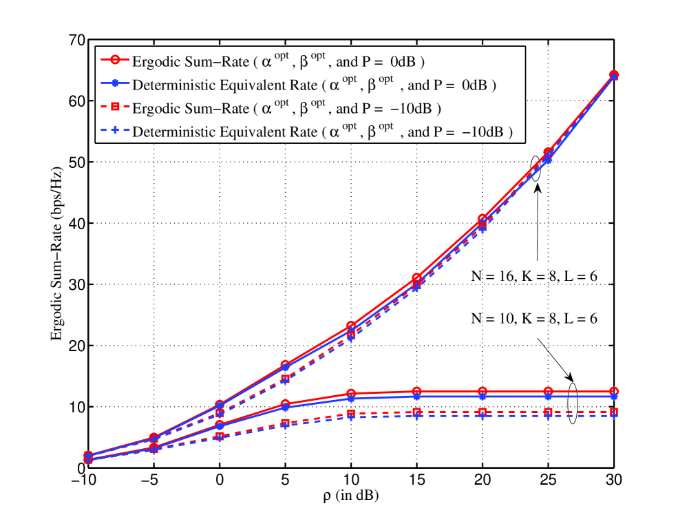
Fig. 2 compares the ergodic sum-rate and its deterministic equivalent result under different interference power thresholds $P\in\{-10{\rm dB},\,0{\rm dB}\}$ and two different antenna configuration cases: $\{N=10,~{}K=8,~{}L=6\}$ and $\{N=16,~{}K=8,~{}L=6\}$. In the simulation, $\{\alpha^{\rm opt},\beta^{\rm opt}\}$ is obtained by using the two-dimensional line search in (14). We find that the deterministic equivalent is accurate under various settings even for systems with a not-so-large number of antennas. In addition, Fig. 2 illustrates that for the case with $\{N=10,~{}K=8,~{}L=6\}$, the sum-rate of the SUs cannot increase linearly in SNR and becomes interference-limited because the sum-rate of the SUs is easily restricted by the average received interference power at each PU, particularly when the number of active users is larger than the number of antennas at the BS, that is, $L+K\geq N$.

Figure 3: Ergodic sum-rate results under various parameters with $P=0$dB and $\{N=16,~{}K=8,~{}L=6\}$.

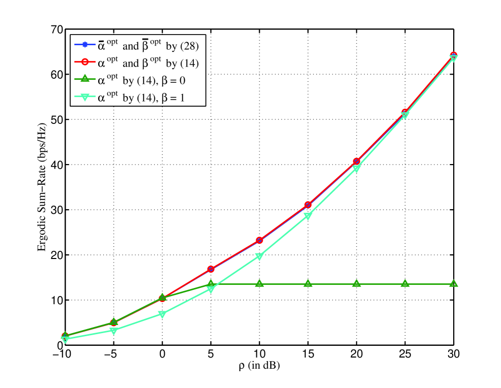
In the above simulations, the best solutions of $\{\alpha^{\rm opt},\beta^{\rm opt}\}$ are calculated by Monte-Carlo averaging over $10^{4}$ independent trials; doing so which clearly results in a high computational cost. To confirm that the optimization based on the deterministic equivalent is not only more computationally efficient but also near-optimal, we compare the ergodic sum-rate of the PP-RZF precoding with $P=0$dB and $\{N=16,~{}K=8,~{}L=6\}$ in Fig. 3 for the following four cases: 1) $\{\overline{\alpha}^{\rm opt},\overline{\beta}^{\rm opt}\}$, 2) $\{\alpha^{\rm opt},\beta^{\rm opt}\}$, 3) $\{\alpha^{\rm opt},\beta=0\}$, and 4) $\{\alpha^{\rm opt},\beta=1\}$. The solution of $\{\overline{\alpha}^{\rm opt},\overline{\beta}^{\rm opt}\}$ is obtained by using the two-dimensional line search in (28). $\{\overline{\alpha}^{\rm opt},\overline{\beta}^{\rm opt}\}$ provides results that are indistinguishable from those achieved by $\{\alpha^{\rm opt},\beta^{\rm opt}\}$, which demonstrates that the optimization based on the deterministic equivalent is promising. Moreover, the performance is significantly improved if the PP-RZF precoding with an appropriate choice of $\{\alpha,\beta\}$ is employed. In the low-SNR regime, the optimal transmission becomes the conventional RZF precoding, whereas the optimal transmission is the PP-RZF precoding with $\beta=1$ in the high-SNR regime.

Figure 4: Optimal $\alpha$ under different the interference power threshold for $\{N=16,~{}K=8,~{}L=6\}$.

Figure 5: Optimal $\beta$ under different interference power threshold for $\{N=16,~{}K=8,~{}L=6\}$.

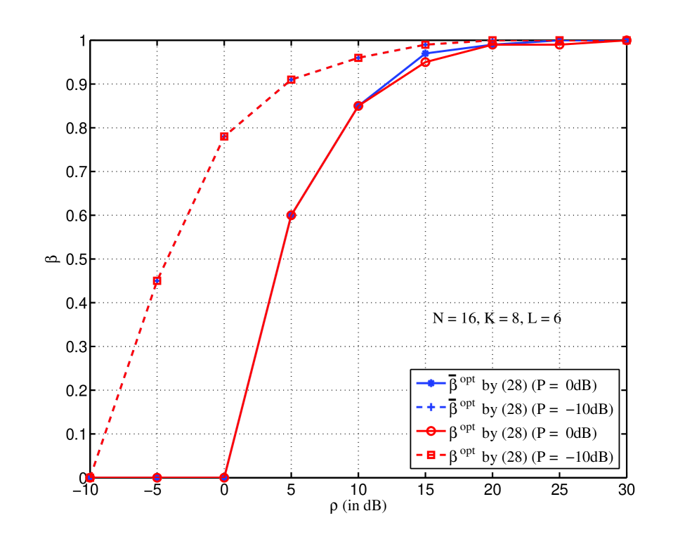
To provide further results on the optimal solutions of $\{\alpha,\beta\}$, Figs. 4 and 5 show the values of $\{\overline{\alpha}^{\rm opt},\overline{\beta}^{\rm opt}\}$, $\{\alpha^{\rm opt},\beta^{\rm opt}\}$ under various settings. We have observed that the optimal parameter $\{\overline{\alpha}^{\rm opt},\overline{\beta}^{\rm opt}\}$ based on the deterministic equivalent result is almost consistent with $\{\alpha^{\rm opt},\beta^{\rm opt}\}$ based on the ergodic sum-rate. Moreover, we have observed that with increasing $\rho$, $\alpha^{\rm opt}$ (or $\overline{\alpha}^{\rm opt}$) tends to monotonically decrease to $0$, whereas $\beta^{\rm opt}$ (or $\overline{\beta}^{\rm opt}$) tends to monotonically increase from $0$ to $1$. These characteristics are expected based on the analysis in Section III.

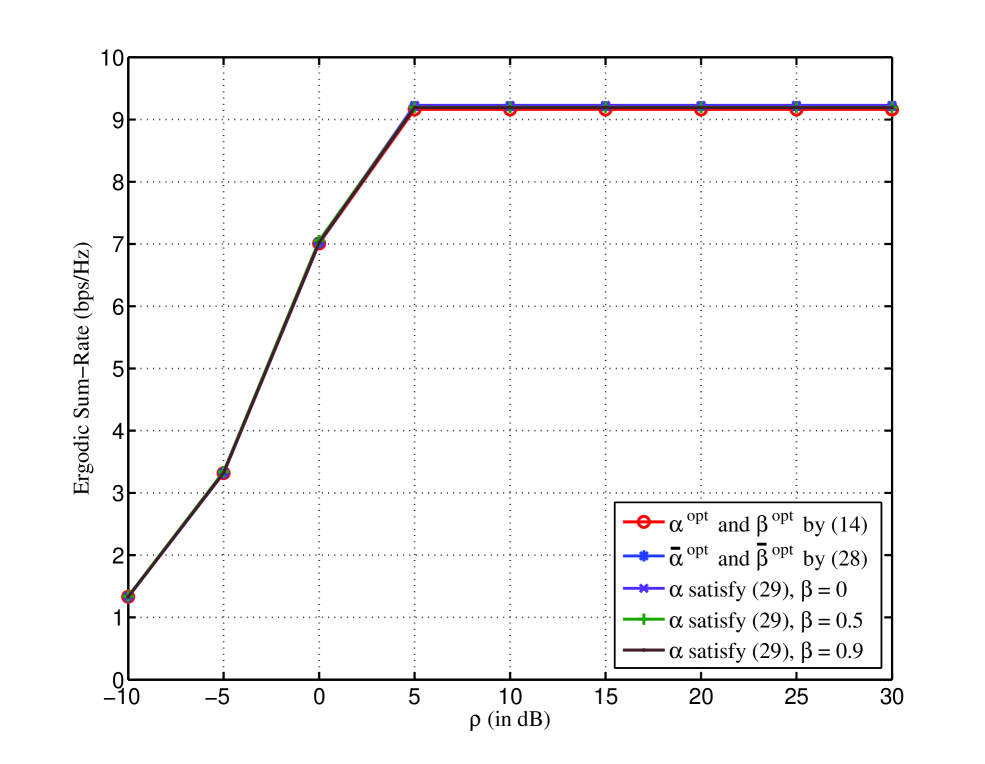
Finally, we confirm the result in Proposition 1. Fig. 6 displays the ergodic sum-rate under various parameter settings with $P=0$dB and $\{N=10,~{}K=8,~{}L=10\}$. We find that when $c_{2}=1$, the parameters that satisfy (29) can achieve the asymptotically optimal sum-rate for any $\beta\in[0,1)$, such that infinitely many asymptotically optimal solutions exist.

Figure 6: Ergodic sum-rate results under various parameters for $P=0$dB and $\{N=10,~{}K=8,~{}L=10\}$.

V Conclusion

By exploiting the recent advancements in large dimensional RMT, we investigated downlink multiuser CR networks that consist of multiple SUs and multiple PUs. The deterministic equivalent of the ergodic sum-rate based on the PP-RZF precoding was derived. Numerical results revealed that the deterministic equivalent sum-rate provides reliable performance predictions even for systems with a not-so-large number of antennas. We thus used the deterministic equivalent result to identify the asymptotically optimal regularization parameter and the asymptotically optimal projection control parameter. In addition, we provided the condition that the regularization parameter and the projection control parameter are asymptotically optimal. Several insights have been gained into the optimal PP-RZF precoding design. A natural extension of this is to consider the PP-RZF precoding under various scenarios, such as spatial correlations and imperfect CSI at the transmitter. However, such development is still ongoing because of mathematical difficulties.

Appendix A: Proof of Theorem 1

To complete this proof, we first introduce the limiting distribution for a new class of random Hermitian matrix in Theorem 2. Such distribution serves as the mathematical basis for the latter derivation. We recall the definition of the Stieltjes transform (see, e.g., [40]). For a Hermitian matrix ${\bf B}_{N}\in{\mathbb{C}}^{N\times N}$, the Stieltjes transform of ${\bf B}_{N}$, is defined as

$$m_{{\bf B}_{N}}(\alpha)=\frac{1}{N}{\sf tr}\left({\bf B}_{N}+\alpha{\bf I}_{N}\right)^{-1}~{}~{}\mbox{for}~{}\alpha\in{{\mathbb{R}}^{+}}.$$

For ease of explanation, we also define the matrix product Stieltjes transform of ${\bf B}_{N}$ as

$$m_{{\bf B}_{N},{\bf Q}}(\alpha)=\frac{1}{N}{\sf tr}{\bf Q}\left({\bf B}_{N}+\alpha{\bf I}_{N}\right)^{-1},$$

where ${\bf Q}$ is any matrix with bounded spectrum norm (with respect to $N$).

Notably, both $m_{{\bf B}_{N}}(\alpha)$ and $m_{{\bf B}_{N},{\bf Q}}(\alpha)$ are functions of $\alpha$, but for ease of notation, $\alpha$ is dropped. In addition, all the subsequent approximations will be performed under the limit ${\mathcal{N}}\rightarrow\infty$, and for ease of expression, $a\asymp b$ denotes that $a-b\xrightarrow{a.s.}0$ as ${\mathcal{N}}\rightarrow\infty$.

Theorem 2

Consider an $N\times N$ matrix of the following form:

$${\bf B}_{N}=\check{{\bf H}}^{H}\check{{\bf H}}=\big{(}{\bf I}_{N}-\beta{\tilde{{\bf W}}}^{H}{\tilde{{\bf W}}}\big{)}{\tilde{{\bf H}}}^{H}{\bf R}_{1}{\tilde{{\bf H}}}\big{(}{\bf I}_{N}-\beta{\tilde{{\bf W}}}^{H}{\tilde{{\bf W}}}\big{)},$$ (31)

where ${\tilde{{\bf W}}}$, ${\tilde{{\bf H}}}$, and ${\bf R}_{1}$ follow the restrictions given by Assumption 1. Then, as ${\mathcal{N}}\rightarrow\infty$, we have

$$m_{{\bf B}_{N},{\bf Q}}\asymp\frac{t_{1}+t_{2}}{\alpha}\frac{1}{N}{\sf tr}{\bf Q},$$ (32)

where $t_{1}=\frac{1-c_{2}}{1+e}$ and $t_{2}=\frac{c_{2}}{1+e(1-\beta)^{2}}$ with $e$ being the unique solution to the fixed point equation

$$e= \frac{1}{N}{\sf tr}{\bf R}_{1}\left(\alpha{\bf I}_{K}+\left(t_{1}+t_{2}(1-\beta)^{2}\right){\bf R}_{1}\right)^{-1}.$$ (33)

Proof: If $c_{2}=1$ (i.e., $N=L$), ${\tilde{{\bf W}}}^{H}{\tilde{{\bf W}}}={\bf I}_{L}$, the result is directly obtained by Lemma 4 (see Appendix C).

We consider the case with $c_{2}<1$. Given that $m_{{\bf B}_{N},{\bf Q}}$ is a function of two random matrices ${\tilde{{\bf W}}}$ and ${\tilde{{\bf H}}}$, we aim to derive an iterative deterministic equivalent [41] of $m_{{\bf B}_{N},{\bf Q}}$. In particular, we first find a function $\tilde{g}_{N}({\tilde{{\bf W}}},\alpha)$, such that $f_{N}(({\tilde{{\bf H}}},{\tilde{{\bf W}}}),\alpha)\asymp\tilde{g}_{N}({\tilde{{\bf W}}},\alpha)$, where $f_{N}(({\tilde{{\bf H}}},{\tilde{{\bf W}}}),\alpha)\triangleq m_{{\bf B}_{N},{\bf Q}}$, and $\tilde{g}_{N}({\tilde{{\bf W}}},\alpha)$ is a function of ${\tilde{{\bf W}}}$ and is independent of $\{{\tilde{{\bf H}}}\}_{N\geq 1}$. Notably, $\tilde{g}_{N}({\tilde{{\bf W}}},\alpha)$ is a deterministic equivalent of $f_{N}(({\tilde{{\bf H}}},{\tilde{{\bf W}}}),\alpha)$ with respect to random matrix sequences $\{{\tilde{{\bf H}}}\}_{N\geq 1}$. Second, we further find a function $g_{N}(\alpha)$, such that $\tilde{g}_{N}({\tilde{{\bf W}}},\alpha)\asymp g_{N}(\alpha)$. Thus, we obtain an iterative deterministic equivalent $g_{N}(\alpha)$ of $f_{N}(({\tilde{{\bf H}}},{\tilde{{\bf W}}}),\alpha)$, i.e., $f_{N}(({\tilde{{\bf H}}},{\tilde{{\bf W}}}),\alpha)\asymp g_{N}(\alpha)$.

When ${\tilde{{\bf W}}}$ is treated as a deterministic matrix, applying Lemma 4 (see Appendix C), we have

$$\frac{1}{N}{\sf tr}{\bf Q}\left({\bf B}_{N}+\alpha{\bf I}_{N}\right)^{-1}\asymp\frac{1}{N}{\sf tr}{\bf Q}\left(\alpha{\bf I}_{N}+\alpha e\big{(}{\bf I}_{N}-\beta{\tilde{{\bf W}}}^{H}{\tilde{{\bf W}}}\big{)}^{2}\right)^{-1},$$ (34)

where

$$e =\frac{1}{N}{\sf tr}{\bf R}_{1}\left(\alpha{\bf I}_{K}+{\tilde{e}}{\bf R}_{1}\right)^{-1},$$ (35)

$${\tilde{e}} =\frac{1}{N}{\sf tr}\big{(}{\bf I}_{N}-\beta{\tilde{{\bf W}}}^{H}{\tilde{{\bf W}}}\big{)}^{2}\left({\bf I}_{N}+e\big{(}{\bf I}_{N}-\beta{\tilde{{\bf W}}}^{H}{\tilde{{\bf W}}}\big{)}^{2}\right)^{-1}.$$ (36)

Notice the fact that $({\tilde{{\bf W}}}^{H}{\tilde{{\bf W}}})^{2}={\tilde{{\bf W}}}^{H}{\tilde{{\bf W}}}$ so (34) and (36) can be written respectively as

$$\frac{1}{N} {\sf tr}{\bf Q}\left(\alpha{\bf I}_{N}+\alpha e\big{(}{\bf I}_{N}-\beta{\tilde{{\bf W}}}^{H}{\tilde{{\bf W}}}\big{)}^{2}\right)^{-1}=\frac{1}{\alpha(\beta^{2}-2\beta)e}\frac{1}{N}{\sf tr}{\bf Q}\big{(}\omega{\bf I}_{N}+{\tilde{{\bf W}}}^{H}{\tilde{{\bf W}}}\big{)}^{-1},$$ (37)

and

$${\tilde{e}}= \frac{1}{(\beta^{2}-2\beta)e}\frac{1}{N}{\sf tr}\big{(}\omega{\bf I}_{N}+{\tilde{{\bf W}}}^{H}{\tilde{{\bf W}}}\big{)}^{-1}+\frac{1}{e}\frac{1}{N}\sum_{l=1}^{L}{\tilde{{\bf w}}}_{l}^{H}\big{(}\omega{\bf I}_{N}+{\tilde{{\bf W}}}^{H}{\tilde{{\bf W}}}\big{)}^{-1}{\tilde{{\bf w}}}_{l},$$ (38)

where $\omega\triangleq\frac{1+e}{(\beta^{2}-2\beta)e}$ and ${\tilde{{\bf w}}}_{l}$ denotes the $l-$th row of ${\tilde{{\bf W}}}$.

Next, we aim to derive the deterministic equivalents of the terms $\frac{1}{N}{\sf tr}{\bf Q}(\omega{\bf I}_{N}+{\tilde{{\bf W}}}^{H}{\tilde{{\bf W}}})^{-1}$ and ${\tilde{{\bf w}}}_{l}^{H}(\omega{\bf I}_{N}+{\tilde{{\bf W}}}^{H}{\tilde{{\bf W}}})^{-1}{\tilde{{\bf w}}}_{l}$. Applying a result of the Haar matrix in Lemma 5 (see Appendix C) to (37) and combing (34), we immediately get (32). Then, we deal with the deterministic equivalent of ${\tilde{{\bf w}}}_{l}^{H}\big{(}\omega{\bf I}_{N}+{\tilde{{\bf W}}}^{H}{\tilde{{\bf W}}}\big{)}^{-1}{\tilde{{\bf w}}}_{l}$. According to the matrix inverse lemma (see, e.g., [42, Lemma 2.1]), we find

$${\tilde{{\bf w}}}_{l}^{H}\big{(}\omega{\bf I}_{N}+{\tilde{{\bf W}}}^{H}{\tilde{{\bf W}}}\big{)}^{-1}{\tilde{{\bf w}}}_{l}=\frac{{\tilde{{\bf w}}}_{l}^{H}\big{(}\omega{\bf I}_{N}+{\tilde{{\bf W}}}_{[l]}^{H}{\tilde{{\bf W}}}_{[l]}\big{)}^{-1}{\tilde{{\bf w}}}_{l}}{1+{\bf w}_{l}^{H}\big{(}\omega{\bf I}_{N}+{\tilde{{\bf W}}}_{[l]}^{H}{\tilde{{\bf W}}}_{[l]}\big{)}^{-1}{\tilde{{\bf w}}}_{l}},$$ (39)

where ${\tilde{{\bf W}}}_{[l]}\triangleq[{\tilde{{\bf w}}}_{1},\ldots,{\tilde{{\bf w}}}_{l-1},{\tilde{{\bf w}}}_{l+1},\ldots,{\tilde{{\bf w}}}_{L}]^{H}\in{\mathbb{C}}^{(L-1)\times N}$. Then, the trace lemma for isometric matrices [43, 44] gives us

$${\tilde{{\bf w}}}_{l}^{H}\big{(}\omega{\bf I}_{N}+{\tilde{{\bf W}}}_{[l]}^{H}{\tilde{{\bf W}}}_{[l]}\big{)}^{-1}{\tilde{{\bf w}}}_{l}\asymp \frac{1}{N-L}{\sf tr}\big{(}{\bf I}_{N}-{\tilde{{\bf W}}}_{[l]}^{H}{\tilde{{\bf W}}}_{[l]}\big{)}\big{(}\omega{\bf I}_{N}+{\tilde{{\bf W}}}_{[l]}^{H}{\tilde{{\bf W}}}_{[l]}\big{)}^{-1}$$

$$= \frac{1+\omega}{N-L}{\sf tr}\big{(}\omega{\bf I}_{N}+{\tilde{{\bf W}}}_{[l]}^{H}{\tilde{{\bf W}}}_{[l]}\big{)}^{-1}-\frac{N}{N-L}.$$ (40)

Now, applying [42, Lemma 2.2] and (72) to (40), we get

$${\tilde{{\bf w}}}_{l}^{H}\big{(}\omega{\bf I}_{N}+{\tilde{{\bf W}}}^{H}{\tilde{{\bf W}}}\big{)}^{-1}{\tilde{{\bf w}}}_{l}\asymp\frac{1}{\omega+1}.$$ (41)

Substituting (41) into (38) and using (72) and (35), we obtain (33).  $\square$

Note that $m_{{\bf B}_{N},{\bf Q}}$, $e$, $t_{1}$, and $t_{2}$ are all functions of $\alpha$ and $\beta$, but for ease of expression, $\alpha$ and $\beta$ are dropped.

Theorem 2 indicates that $m_{{\bf B},{\bf Q}}$ can be approximated by its deterministic equivalent $\frac{t_{1}+t_{2}}{\alpha}\frac{1}{N}{\sf tr}{\bf Q}$ without knowing the actual realization of channel random components. The deterministic equivalent is analytical and is much easier to compute than ${\sf E}_{{\bf B}}\{m_{{\bf B},{\bf Q}}\}$, which requires time-consuming Monte-Carlo simulations. Motivated by this result in the large system limit, we aim to derive the deterministic equivalent of $\gamma_{k}$.

The SINR $\gamma_{k}$ in (II-A) consists of three terms: $(\textrm{i})$ the signal power $|{\bf h}_{k}^{H}(\check{{\bf H}}^{H}\check{{\bf H}}+\alpha{\bf I}_{N})^{-1}\check{{\bf h}}_{k}|^{2}$, $(\textrm{ii})$ the interference power ${\bf h}_{k}^{H}(\check{{\bf H}}^{H}\check{{\bf H}}+\alpha{\bf I}_{N})^{-1}\check{{\bf H}}_{[k]}^{H}{\bf P}_{[k]}\check{{\bf H}}_{[k]}(\check{{\bf H}}^{H}\check{{\bf H}}+\alpha{\bf I}_{N})^{-1}{\bf h}_{k}$, and $(\textrm{iii})$ the noise power $\nu$. Using Theorem 2, we establish the following three lemmas to derive the deterministic equivalent of each term, whose proofs are detailed in Appendices B-I, B-II, and B-III, successively.

Lemma 1

Under the assumption of Theorem 2, as ${\mathcal{N}}\rightarrow\infty$, we have

$${\bf h}_{k}^{H}\left(\check{{\bf H}}^{H}\check{{\bf H}}+\alpha{\bf I}_{N}\right)^{-1}\check{{\bf h}}_{k}\asymp\overline{a}_{k},$$ (42)

where $\overline{a}_{k}$ has been obtained by (16a).

Lemma 2

Under the assumption of Theorem 2, as ${\mathcal{N}}\rightarrow\infty$, we have

$${\bf h}_{k}^{H}\left(\check{{\bf H}}^{H}\check{{\bf H}}+\alpha{\bf I}_{N}\right)^{-1}\check{{\bf H}}_{[k]}^{H}\check{{\bf H}}_{[k]}\left(\check{{\bf H}}^{H}\check{{\bf H}}+\alpha{\bf I}_{N}\right)^{-1}{\bf h}_{k}\asymp\overline{b}_{k},$$ (43)

where $\overline{b}_{k}$ has been obtained by (16b).

Lemma 3

Under the assumption of Theorem 2, as ${\mathcal{N}}\rightarrow\infty$, we have

$$\nu\asymp\overline{\nu},$$ (44)

where $\overline{\nu}$ can be obtained by (16c) for Case I and by (18) for Case II.

According to Lemma 1, Lemma 2, and Lemma 3, we obtain the deterministic equivalent $\overline{\gamma}_{k}$ of $\gamma_{k}$ in (15). The proof is then completed.

Appendix B: Proofs of Lemma 1, Lemma 2, and Lemma 3

B-I: Proof of Lemma 1

We start from an application of the matrix inverse lemma [42, Lemma 2.1] to the signal term, which results in

$${\bf h}_{k}^{H}\left(\check{{\bf H}}^{H}\check{{\bf H}}+\alpha{\bf I}_{N}\right)^{-1}\check{{\bf h}}_{k}=\frac{{\bf h}_{k}^{H}\big{(}\check{{\bf H}}_{[k]}^{H}\check{{\bf H}}_{[k]}+\alpha{\bf I}_{N}\big{)}^{-1}\check{{\bf h}}_{k}}{1+\check{{\bf h}}_{k}^{H}\big{(}\check{{\bf H}}_{[k]}^{H}\check{{\bf H}}_{[k]}+\alpha{\bf I}_{N}\big{)}^{-1}\check{{\bf h}}_{k}}.$$ (45)

Using [42, Lemma 2.3 and Lemma 2.2], we obtain

$${\bf h}_{k}^{H}\left(\check{{\bf H}}_{[k]}^{H}\check{{\bf H}}_{[k]}+\alpha{\bf I}_{N}\right)^{-1}\check{{\bf h}}_{k}\asymp r_{1,k}\frac{1}{N}{\sf tr}\left(\check{{\bf H}}^{H}\check{{\bf H}}+\alpha{\bf I}_{N}\right)^{-1}-r_{1,k}\beta\frac{1}{N}{\sf tr}{\bf W}^{H}{\bf W}\left(\check{{\bf H}}^{H}\check{{\bf H}}+\alpha{\bf I}_{N}\right)^{-1}.$$ (46)

Similarly,

$$\check{{\bf h}}_{k}^{H}\left(\check{{\bf H}}_{[k]}^{H}\check{{\bf H}}_{[k]}+\alpha{\bf I}_{N}\right)^{-1}\check{{\bf h}}_{k}$$

$$\asymp r_{1,k}\frac{1}{N}{\sf tr}\left(\check{{\bf H}}^{H}\check{{\bf H}}+\alpha{\bf I}_{N}\right)^{-1}+r_{1,k}(\beta^{2}-2\beta)\frac{1}{N}{\sf tr}{\bf W}^{H}{\bf W}\left(\check{{\bf H}}^{H}\check{{\bf H}}+\alpha{\bf I}_{N}\right)^{-1}.$$ (47)

According to Theorem 2, we have

$$\frac{1}{N}{\sf tr}\left(\check{{\bf H}}^{H}\check{{\bf H}}+\alpha{\bf I}_{N}\right)^{-1}\asymp\frac{t_{1}+t_{2}}{\alpha}.$$ (48)

Noticing that ${\bf W}^{H}{\bf W}={\tilde{{\bf W}}}^{H}{\tilde{{\bf W}}}$ and by using the same approach as (38), we obtain

$$\frac{1}{N}{\sf tr}{\bf W}^{H}{\bf W}\big{(}\check{{\bf H}}^{H}\check{{\bf H}}+\alpha{\bf I}_{N}\big{)}^{-1}\asymp \frac{1}{\alpha(\beta^{2}-2\beta)e}\frac{1}{N}\sum_{l=1}^{L}{\tilde{{\bf w}}}_{l}^{H}\big{(}\omega{\bf I}_{N}+{\tilde{{\bf W}}}^{H}{\tilde{{\bf W}}}\big{)}^{-1}{\tilde{{\bf w}}}_{l}\asymp\frac{t_{2}}{\alpha}.$$ (49)

Substituting (48) and (49) into (46) and (47), we obtain

$${\bf h}_{k}^{H}\left(\check{{\bf H}}_{[k]}^{H}\check{{\bf H}}_{[k]}+\alpha{\bf I}_{N}\right)^{-1}\check{{\bf h}}_{k} \asymp\frac{r_{1,k}\left(t_{1}+t_{2}(1-\beta)\right)}{\alpha},$$ (50)

$$\check{{\bf h}}_{k}^{H}\left(\check{{\bf H}}_{[k]}^{H}\check{{\bf H}}_{[k]}+\alpha{\bf I}_{N}\right)^{-1}\check{{\bf h}}_{k} \asymp\frac{r_{1,k}\left(t_{1}+t_{2}(1-\beta)^{2}\right)}{\alpha}.$$ (51)

Consequently, the expression of (45), together with (50) and (51), yields (42).

B-II: Proof of Lemma 2

Using the fact that ${\bf A}^{-1}-{\bf D}^{-1}=-{\bf A}^{-1}({\bf A}-{\bf D}){\bf D}^{-1}$, we have

$${\bf h}_{k}^{H}\left(\check{{\bf H}}^{H}\check{{\bf H}}+\alpha{\bf I}_{N}\right)^{-1}\check{{\bf H}}_{[k]}^{H}\check{{\bf H}}_{[k]}\left(\check{{\bf H}}^{H}\check{{\bf H}}+\alpha{\bf I}_{N}\right)^{-1}{\bf h}_{k}$$

$$= {\bf h}_{k}^{H}\left(\check{{\bf H}}^{H}\check{{\bf H}}+\alpha{\bf I}_{N}\right)^{-1}{\bf h}_{k}-\alpha{\bf h}_{k}^{H}\left(\check{{\bf H}}_{[k]}^{H}\check{{\bf H}}_{[k]}+\alpha{\bf I}_{N}\right)^{-1}\left(\check{{\bf H}}^{H}\check{{\bf H}}+\alpha{\bf I}_{N}\right)^{-1}{\bf h}_{k}$$

$$-{\bf h}_{k}^{H}\left(\check{{\bf H}}^{H}\check{{\bf H}}+\alpha{\bf I}_{N}\right)^{-1}\check{{\bf h}}_{k}\check{{\bf h}}_{k}^{H}\left(\check{{\bf H}}^{H}\check{{\bf H}}+\alpha{\bf I}_{N}\right)^{-1}{\bf h}_{k}$$

$$+\alpha{\bf h}_{k}^{H}\left(\check{{\bf H}}^{H}\check{{\bf H}}+\alpha{\bf I}_{N}\right)^{-1}\check{{\bf h}}_{k}\check{{\bf h}}_{k}^{H}\left(\check{{\bf H}}_{[k]}^{H}\check{{\bf H}}_{[k]}+\alpha{\bf I}_{N}\right)^{-1}\left(\check{{\bf H}}^{H}\check{{\bf H}}+\alpha{\bf I}_{N}\right)^{-1}{\bf h}_{k}.$$ (52)

Applying the matrix inverse lemma, we obtain

$${\bf h}_{k}^{H}\left(\check{{\bf H}}^{H}\check{{\bf H}}+\alpha{\bf I}_{N}\right)^{-1}{\bf h}_{k}$$

$$= {\bf h}_{k}^{H}\left(\check{{\bf H}}_{[k]}^{H}\check{{\bf H}}_{[k]}+\alpha{\bf I}_{N}\right)^{-1}{\bf h}_{k}-\frac{{\bf h}_{k}^{H}\big{(}\check{{\bf H}}_{[k]}^{H}\check{{\bf H}}_{[k]}+\alpha{\bf I}_{N}\big{)}^{-1}\check{{\bf h}}_{k}\check{{\bf h}}_{k}^{H}\big{(}\check{{\bf H}}_{[k]}^{H}\check{{\bf H}}_{[k]}+\alpha{\bf I}_{N}\big{)}^{-1}{\bf h}_{k}}{1+\check{{\bf h}}_{k}^{H}\big{(}\check{{\bf H}}_{[k]}^{H}\check{{\bf H}}_{[k]}+\alpha{\bf I}_{N}\big{)}^{-1}\check{{\bf h}}_{k}}.$$ (53)

Similarly,

$${\bf h}_{k}^{H}\big{(}\check{{\bf H}}_{[k]}^{H}\check{{\bf H}}_{[k]}+\alpha{\bf I}_{N}\big{)}^{-1}\left(\check{{\bf H}}^{H}\check{{\bf H}}+\alpha{\bf I}_{N}\right)^{-1}{\bf h}_{k}$$

$$= {\bf h}_{k}^{H}\left(\check{{\bf H}}_{[k]}^{H}\check{{\bf H}}_{[k]}+\alpha{\bf I}_{N}\right)^{-2}{\bf h}_{k}-\frac{{\bf h}_{k}^{H}\big{(}\check{{\bf H}}_{[k]}^{H}\check{{\bf H}}_{[k]}+\alpha{\bf I}_{N}\big{)}^{-2}\check{{\bf h}}_{k}\check{{\bf h}}_{k}^{H}\big{(}\check{{\bf H}}_{[k]}^{H}\check{{\bf H}}_{[k]}+\alpha{\bf I}_{N}\big{)}^{-1}{\bf h}_{k}}{1+\check{{\bf h}}_{k}^{H}\big{(}\check{{\bf H}}_{[k]}^{H}\check{{\bf H}}_{[k]}+\alpha{\bf I}_{N}\big{)}^{-1}\check{{\bf h}}_{k}},$$ (54)

and

$$\check{{\bf h}}_{k}^{H}\big{(}\check{{\bf H}}_{[k]}^{H}\check{{\bf H}}_{[k]}+\alpha{\bf I}_{N}\big{)}^{-1}\big{(}\check{{\bf H}}^{H}\check{{\bf H}}+\alpha{\bf I}_{N}\big{)}^{-1}{\bf h}_{k}$$

$$= \check{{\bf h}}_{k}^{H}\left(\check{{\bf H}}_{[k]}^{H}\check{{\bf H}}_{[k]}+\alpha{\bf I}_{N}\right)^{-2}{\bf h}_{k}-\frac{\check{{\bf h}}_{k}^{H}\big{(}\check{{\bf H}}_{[k]}^{H}\check{{\bf H}}_{[k]}+\alpha{\bf I}_{N}\big{)}^{-2}\check{{\bf h}}_{k}\check{{\bf h}}_{k}^{H}\big{(}\check{{\bf H}}_{[k]}^{H}\check{{\bf H}}_{[k]}+\alpha{\bf I}_{N}\big{)}^{-1}{\bf h}_{k}}{1+\check{{\bf h}}_{k}^{H}\big{(}\check{{\bf H}}_{[k]}^{H}\check{{\bf H}}_{[k]}+\alpha{\bf I}_{N}\big{)}^{-1}\check{{\bf h}}_{k}}.$$ (55)

According to Theorem 2, we have

$${\bf h}_{k}^{H}\left(\check{{\bf H}}_{[k]}^{H}\check{{\bf H}}_{[k]}+\alpha{\bf I}_{N}\right)^{-1}{\bf h}_{k}\asymp\frac{r_{1,k}\left(t_{1}+t_{2}\right)}{\alpha}.$$ (56)

Noticing that

$${\bf h}_{k}^{H}\left(\check{{\bf H}}_{[k]}^{H}\check{{\bf H}}_{[k]}+\alpha{\bf I}_{N}\right)^{-2}{\bf h}_{k}=-\frac{\partial}{\partial\alpha}{\bf h}_{k}^{H}\left(\check{{\bf H}}_{[k]}^{H}\check{{\bf H}}_{[k]}+\alpha{\bf I}_{N}\right)^{-1}{\bf h}_{k},$$

we thus obtain

$${\bf h}_{k}^{H}\left(\check{{\bf H}}_{[k]}^{H}\check{{\bf H}}_{[k]}+\alpha{\bf I}_{N}\right)^{-2}{\bf h}_{k}\asymp-r_{1,k}\frac{\partial}{\partial\alpha}\left(\frac{t_{1}+t_{2}}{\alpha}\right).$$ (57)

Similarly, combining (50) and (51) yields

$$\check{{\bf h}}_{k}^{H}\left(\check{{\bf H}}_{[k]}^{H}\check{{\bf H}}_{[k]}+\alpha{\bf I}_{N}\right)^{-2}{\bf h}_{k} \asymp-r_{1,k}\frac{\partial}{\partial\alpha}\left(\frac{t_{1}+(1-\beta)t_{2}}{\alpha}\right),$$ (58)

$$\check{{\bf h}}_{k}^{H}\left(\check{{\bf H}}_{[k]}^{H}\check{{\bf H}}_{[k]}+\alpha{\bf I}_{N}\right)^{-2}\check{{\bf h}}_{k} \asymp-r_{1,k}\frac{\partial}{\partial\alpha}\left(\frac{t_{1}+(1-\beta)^{2}t_{2}}{\alpha}\right).$$ (59)

Substituting (50), (51), (56), (57), (58), and (59) into (53), (54), and (55), and combining (42) and (52), we obtain (43).

B-III: Proof of Lemma 3

From (11), we first have

$$\frac{1}{N}{\sf tr}\left(\check{{\bf H}}^{H}\check{{\bf H}}+\alpha{\bf I}_{N}\right)^{-1}\check{{\bf H}}^{H}\check{{\bf H}}\left(\check{{\bf H}}^{H}\check{{\bf H}}+\alpha{\bf I}_{N}\right)^{-1}$$

$$= \frac{1}{N}{\sf tr}\left(\check{{\bf H}}^{H}\check{{\bf H}}+\alpha{\bf I}_{N}\right)^{-1}-\alpha\frac{1}{N}{\sf tr}\left(\check{{\bf H}}^{H}\check{{\bf H}}+\alpha{\bf I}_{N}\right)^{-2},$$ (60)

which, together with Theorem 2, yields

$$\frac{1}{N}{\sf tr}\left(\check{{\bf H}}^{H}\check{{\bf H}}+\alpha{\bf I}_{N}\right)^{-1}\check{{\bf H}}^{H}\check{{\bf H}}\left(\check{{\bf H}}^{H}\check{{\bf H}}+\alpha{\bf I}_{N}\right)^{-1}\asymp\frac{\partial t_{1}}{\partial\alpha}+\frac{\partial t_{2}}{\partial\alpha}.$$ (61)

For Case I, we have

$${\bf f}_{l}^{H}\left(\check{{\bf H}}^{H}\check{{\bf H}}+\alpha{\bf I}_{N}\right)^{-1}\check{{\bf H}}^{H}\check{{\bf H}}\left(\check{{\bf H}}^{H}\check{{\bf H}}+\alpha{\bf I}_{N}\right)^{-1}{\bf f}_{l}$$

$$= {\bf f}_{l}^{H}\left(\check{{\bf H}}^{H}\check{{\bf H}}+\alpha{\bf I}_{N}\right)^{-1}{\bf f}_{l}-\alpha{\bf f}_{l}^{H}\left(\check{{\bf H}}^{H}\check{{\bf H}}+\alpha{\bf I}_{N}\right)^{-2}{\bf f}_{l},$$ (62)

where $l=1,\ldots,L$. From (34) and (37), we obtain

$${\bf f}_{l}^{H}\left(\check{{\bf H}}^{H}\check{{\bf H}}+\alpha{\bf I}_{N}\right)^{-1}{\bf f}_{l}\asymp\frac{1}{\alpha(\beta^{2}-2\beta)e}{\sf tr}{\bf f}_{l}{\bf f}_{l}^{H}\left(\omega{\bf I}_{N}+{\bf W}^{H}{\bf W}\right)^{-1}.$$ (63)

Noticing the fact that ${\bf W}=({\bf F}{\bf F}^{H})^{-\frac{1}{2}}{\bf F}$, by using the matrix inversion formula, we obtain

$${\sf tr}{\bf f}_{l}{\bf f}_{l}^{H}\left(\omega{\bf I}_{N}+{\bf W}^{H}{\bf W}\right)^{-1}= {\sf tr}{\bf f}_{l}{\bf f}_{l}^{H}\left(\omega^{-1}{\bf I}_{N}-\omega^{-1}{\bf F}^{H}\left({\bf F}{\bf F}^{H}+\omega^{-1}{\bf F}{\bf F}^{H}\right)^{-1}{\bf F}\omega^{-1}\right)$$

$$= \frac{1}{\omega+1}{\sf tr}{\bf f}_{l}{\bf f}_{l}^{H}\asymp\frac{r_{2,l}}{\omega+1}.$$ (64)

As a result,

$${\bf f}_{l}^{H}\left(\check{{\bf H}}^{H}\check{{\bf H}}+\alpha{\bf I}_{N}\right)^{-1}{\bf f}_{l}\asymp\frac{r_{2,l}t_{2}}{c_{2}\alpha}.$$ (65)

Combining this with (62), we obtain

$${\bf f}_{l}^{H}\left(\check{{\bf H}}^{H}\check{{\bf H}}+\alpha{\bf I}_{N}\right)^{-1}\check{{\bf H}}^{H}\check{{\bf H}}\left(\check{{\bf H}}^{H}\check{{\bf H}}+\alpha{\bf I}_{N}\right)^{-1}{\bf f}_{l}\asymp\frac{r_{2,l}}{c_{2}}\frac{\partial t_{2}}{\partial\alpha}.$$ (66)

From (61) and (66), the proof of (16c) can be accomplished using

$$\frac{1}{N}{\sf tr}\big{(}\check{{\bf H}}^{H}\check{{\bf H}}+\alpha{\bf I}_{N}\big{)}^{-1}\check{{\bf H}}^{H}\check{{\bf H}}\big{(}\check{{\bf H}}^{H}\check{{\bf H}}+\alpha{\bf I}_{N}\big{)}^{-1}$$

$$\asymp {\sf E}\left\{\frac{1}{N}{\sf tr}\big{(}\check{{\bf H}}^{H}\check{{\bf H}}+\alpha{\bf I}_{N}\big{)}^{-1}\check{{\bf H}}^{H}\check{{\bf H}}\big{(}\check{{\bf H}}^{H}\check{{\bf H}}+\alpha{\bf I}_{N}\big{)}^{-1}\right\},$$ (67a)

$${\bf f}_{l}^{H}\big{(}\check{{\bf H}}^{H}\check{{\bf H}}+\alpha{\bf I}_{N}\big{)}^{-1}\check{{\bf H}}^{H}\check{{\bf H}}\big{(}\check{{\bf H}}^{H}\check{{\bf H}}+\alpha{\bf I}_{N}\big{)}^{-1}{\bf f}_{l}$$

$$\asymp {\sf E}\left\{{\bf f}_{l}^{H}\big{(}\check{{\bf H}}^{H}\check{{\bf H}}+\alpha{\bf I}_{N}\big{)}^{-1}\check{{\bf H}}^{H}\check{{\bf H}}\big{(}\check{{\bf H}}^{H}\check{{\bf H}}+\alpha{\bf I}_{N}\big{)}^{-1}{\bf f}_{l}\right\}.$$ (67b)

By using the martingale approach, we can prove (67) (See [45] for a similar application).

Similarly, for Case II, we have

$${\sf E}\left\{{\sf tr}{\bf F}\big{(}\check{{\bf H}}^{H}\check{{\bf H}}+\alpha{\bf I}_{N}\big{)}^{-1}\check{{\bf H}}^{H}\check{{\bf H}}\big{(}\check{{\bf H}}^{H}\check{{\bf H}}+\alpha{\bf I}_{N}\big{)}^{-1}{\bf F}^{H}\right\}\asymp\frac{{\sf tr}{\bf R}_{2}}{c_{2}}\frac{\partial t_{2}}{\partial\alpha}.$$ (68)

Therefore, we obtain (18).

Appendix C: Related Lemmas

In this appendix, we provide some lemmas needed in the proof of Appendix A.

Lemma 4

Let ${\bf X}\equiv[\frac{1}{\sqrt{N}}X_{ij}]\in{\mathbb{C}}^{N\times K}$, where $X_{ij}$’s are i.i.d. with zero mean, unit variance and finite $4$-th order moment. In addition, let ${\bf Q}\in{\mathbb{C}}^{N\times N}$, ${\bf T}\in{\mathbb{C}}^{N\times N}$, and ${\bf R}\in{\mathbb{C}}^{K\times K}$ be nonnegative definite matrices with uniformly bounded spectral norm (with respect to $N$, $N$, and $K$, respectively). Consider an $N\times N$ matrix of the form ${\bf B}_{N}={\bf T}^{\frac{1}{2}}{\bf X}{\bf R}{\bf X}^{H}{\bf T}^{\frac{1}{2}}$. Define $c_{1}=N/K$. Then, as $K,N\rightarrow\infty$ such that $0<\lim\inf_{N}c_{1}\leq\lim\sup_{N}c_{1}<\infty$, the following holds for any $\omega\in{\mathbb{R}}^{+}$:

$$\frac{1}{N}{\sf tr}{\bf Q}\big{(}{\bf B}_{N}+\omega{\bf I}_{N}\big{)}^{-1}\asymp\frac{1}{N}{\sf tr}{\bf Q}\left(\omega{\bf I}_{N}+\omega e{\bf T}\right)^{-1},$$ (69)

where $e$ is given as the unique solution to the fixed-point equations

$$e =\frac{1}{N}{\sf tr}{\bf R}(\omega{\bf I}_{K}+{\tilde{e}}{\bf R})^{-1},$$

$${\tilde{e}} =\frac{1}{N}{\sf tr}{\bf T}({\bf I}_{N}+e{\bf T})^{-1}.$$

Proof: As a special case of [46, Theorem 1] or [21, Theorem 1], the result can be obtained immediately.  $\square$

Lemma 5

Let ${\bf Q}\in{\mathbb{C}}^{N\times N}$ be a nonnegative definite matrix with uniformly bounded spectral norm (with respect to $N$) and ${\tilde{{\bf W}}}\in{\mathbb{C}}^{L\times N}$ be $L\leq N$ rows of an $N\times N$ Haar-distributed unitary random matrix. Define $c_{2}=L/N$. Then, as $L,N\rightarrow\infty$ such that $0<\lim\inf_{N}c_{2}\leq\lim\sup_{N}c_{2}\leq 1$, the following holds for any $\omega\in{\mathbb{R}}^{+}$:

$$\frac{1}{N}{\sf tr}{\bf Q}\big{(}{\tilde{{\bf W}}}^{H}{\tilde{{\bf W}}}+\omega{\bf I}_{N}\big{)}^{-1}\asymp\left(\frac{c_{2}}{\omega+1}+\frac{1-c_{2}}{\omega}\right)\frac{1}{N}{\sf tr}{\bf Q}.$$ (70)

Proof: Since ${\tilde{{\bf W}}}^{H}{\tilde{{\bf W}}}={\bf I}_{L}$ for $c_{2}=1$ (i.e., $N=L$), (70) evidently holds. We assume $c_{2}<1$ in the following proof. Firstly, we consider a special case with ${\bf Q}={\bf I}$. Using the identity of the Stieltjes transform [29, Lemma 3.1] , we have

$$\frac{1}{N}{\sf tr}\big{(}{\tilde{{\bf W}}}^{H}{\tilde{{\bf W}}}+\omega{\bf I}_{N}\big{)}^{-1}=\frac{c_{2}}{L}{\sf tr}\big{(}{\tilde{{\bf W}}}{\tilde{{\bf W}}}^{H}+\omega{\bf I}_{L}\big{)}^{-1}+\frac{1-c_{2}}{\omega}.$$ (71)

Notice that the rows of ${\tilde{{\bf W}}}$ are orthogonal and hence ${\tilde{{\bf W}}}{\tilde{{\bf W}}}^{H}={\bf I}_{L}$. Therefore,

$$\frac{1}{N}{\sf tr}\big{(}{\tilde{{\bf W}}}^{H}{\tilde{{\bf W}}}+\omega{\bf I}_{N}\big{)}^{-1}\asymp\delta\triangleq\frac{c_{2}}{\omega+1}+\frac{1-c_{2}}{\omega}.$$ (72)

Next, for any nonnegative definite matrix with uniformly bounded spectral norm (with respect to $N$) ${\bf Q}$, we have

$$\frac{1}{N}{\sf tr}{\bf Q}\big{(}{\tilde{{\bf W}}}^{H}{\tilde{{\bf W}}}+\omega{\bf I}_{N}\big{)}^{-1}-\delta\frac{1}{N}{\sf tr}{\bf Q}$$

$$= \left(1-\delta\omega\right)\frac{1}{N}{\sf tr}{\bf Q}\big{(}{\tilde{{\bf W}}}^{H}{\tilde{{\bf W}}}+\omega{\bf I}_{N}\big{)}^{-1}-\delta\sum_{l=1}^{L}{\bf w}_{l}^{H}{\bf Q}\big{(}{\tilde{{\bf W}}}^{H}{\tilde{{\bf W}}}+\omega{\bf I}_{N}\big{)}^{-1}{\bf w}_{l},$$ (73)

where the first equality follows from the resolvent identity: ${\bf A}^{-1}-{\bf B}^{-1}={\bf A}^{-1}({\bf B}-{\bf A}){\bf B}^{-1}$ for invertible matrices ${\bf A}$ and ${\bf B}$. Using the matrix inverse lemma [42, Lemma 2.1], the trace lemma for isometric matrices [43, 44], and the fact that ${\bf Q}$ has uniformly bounded spectral norm (with respect to $N$), we obtain

$$\sum_{l=1}^{L}{\bf w}_{l}^{H}{\bf Q}\big{(}{\tilde{{\bf W}}}^{H}{\tilde{{\bf W}}}+\omega{\bf I}_{N}\big{)}^{-1}{\bf w}_{l}= \sum_{l=1}^{L}\frac{{\bf w}_{l}^{H}{\bf Q}\big{(}{\tilde{{\bf W}}}^{H}_{[l]}{\tilde{{\bf W}}}_{[l]}+\omega{\bf I}_{N}\big{)}^{-1}{\bf w}_{l}}{1+{\bf w}_{l}^{H}\big{(}{\tilde{{\bf W}}}^{H}_{[l]}{\tilde{{\bf W}}}_{[l]}+\omega{\bf I}_{N}\big{)}^{-1}{\bf w}_{l}}$$

$$\asymp c_{2}\frac{(1+\omega)\frac{1}{N}{\sf tr}{\bf Q}\big{(}{\tilde{{\bf W}}}^{H}{\tilde{{\bf W}}}+\omega{\bf I}_{N}\big{)}^{-1}-\frac{1}{N}{\sf tr}{\bf Q}}{(1+\omega)\frac{1}{N}{\sf tr}\big{(}{\tilde{{\bf W}}}^{H}{\tilde{{\bf W}}}+\omega{\bf I}_{N}\big{)}^{-1}-c_{2}}.$$ (74)

Substituting (74) into (73), and combining (72), yields

$$\frac{(1+\omega)\delta\left(\frac{1}{N}{\sf tr}{\bf Q}\big{(}{\tilde{{\bf W}}}^{H}{\tilde{{\bf W}}}+\omega{\bf I}_{N}\big{)}^{-1}-\delta\frac{1}{N}{\sf tr}{\bf Q}\right)}{(1+\omega)\delta-c_{2}}\asymp 0.$$ (75)

Therefore, we get (70).  $\square$

References

- [1] J. Mitola and G. Q. Maguire, “Cognitive radio: Making software radio more personal,” IEEE Personal Commun. Mag., vol. 6, no. 4, pp. 13–18, Aug. 1999.
- [2] K. B. Letaief and W. Zhang, “Cooperative communications for cognitive radio networks,” Proceedings of the IEEE, vol. 97, no. 5, pp. 878–893, May 2009.
- [3] A. Goldsmith, S. Jafar, I. Maric, and S. Srinivasa, “Breaking spectrum gridlock with cognitive radios: An information theoretic perspective,” Proceedings of the IEEE, vol. 97, no. 5, pp. 894–914, May 2009.
- [4] Y.-C. Liang, K.-C. Chen, G. Y. Li, and P. Mahonen, “Cognitive radio networking and communications: An overview,” IEEE Trans. Veh. Technol., vol. 60, no. 7, pp. 3386–3407, Sep. 2011.
- [5] J. Kim, Y. Shin, T. W. Ban, and R. Schober, “Effect of spectrum sensing reliability on the capacity of multiuser uplink cognitive radio systems,” IEEE Trans. Veh. Technol., vol. 60, no. 9, pp. 4349–4362, Nov. 2011.
- [6] G. Zheng, K.-K. Wong, and B. Ottersten, “Robust cognitive beamforming with bounded channel uncertainties,” IEEE Trans. Sig. Proc., vol. 57, no. 12, pp. 4871–4881, Dec. 2009.
- [7] S. Huang, X. Liu, and Z. Ding, “Decentralized cognitive radio control based on inference from primary link control information,” IEEE J. Sel. Areas Commun., vol. 29, no. 2, pp. 394–406, Feb. 2011.
- [8] R. Zhang and Y.-C. Liang, “Exploiting multi-antennas for opportunistic spectrum sharing in cognitive radio networks,” IEEE J. Sel. Topics Sig. Proc., vol. 2, no. 1, pp. 88–102, Feb. 2008.
- [9] K. Hamdi, W. Zhang, and K. B. Letaief, “Opportunistic spectrum sharing in cognitive MIMO wireless networks,” IEEE Trans. Wireless Commun., vol. 8, no. 8, pp. 4098–4109, Aug. 2009.
- [10] Y. Y. He and S. Dey, “Sum rate maximization for cognitive MISO broadcast channels: Beamforming design and large systems analysis,” IEEE Trans. Wireless Commun., vol. 13, no. 5, pp. 2383–2401, May 2014.
- [11] ——, “Weighted sum rate maximization for cognitive MISO broadcast channel: Large system analysis,” in Proc. ICASSP, Vancouver, Canada, May 2013, pp. 4873–4877.
- [12] X. Chen and C. Yuen, “Efficient resource allocation in rateless coded MU-MIMO cognitive radio network with QoS provisioning and limited feedback,” IEEE Trans. Veh. Technol., vol. 62, no. 1, pp. 395–399, Jan. 2013.
- [13] G. Caire and S. Shamai, “On the achievable throughput of a multiantenna Gaussian broadcast channel,” IEEE Trans. Inf. Theory, vol. 49, no. 7, pp. 1691–1706, Jul. 2003.
- [14] D. Samardzija, H. Huang, T. Sizer, and R. Valenzuela, “Experimental downlink multiuser MIMO system with distributed and coherently coordinated transmit antennas,” in Proc. IEEE Int. Conf. on Commun. (ICC), Glasgow, Scotland, Jun. 2007, pp. 5365–5370.
- [15] R. Irmer, H.-P. Mayer, A. Weber, V. Braun, M. Schmidt, M. Ohm, N. Ahr, A. Zoch, C. Jandura, P. Marsch, and G. Fettweis, “Multisite field trial for LTE and advanced concepts,” IEEE Commun. Mag., vol. 47, no. 2, pp. 92–98, Feb. 2009.
- [16] H. A. Suraweera, H. Q. Ngo, T. Q. Duong, C. Yuen, and E. G. Larsson, “Multi-pair amplify-and-forward relaying with large antenna arrays,” in Proc. IEEE Int. Conf. on Commun. (ICC), Budapest, Hungary, Jun. 2013, pp. 3228–3233.
- [17] M. Joham, K. Kusume, M. H. Gzara, W. Utschick, and J. A. Nossek, “Transmit Wiener filter for the downlink of TDDDS-CDMA systems,” in Proc. IEEE 7th Int. Symp. Spread-Spectrum Tech. Appl. (ISSSTA), vol. 1, 2002, pp. 9–13.
- [18] C. B. Peel, B. M. Hochwald, and A. L. Swindlehurst, “A vector-perturbation technique for near-capacity multiantenna multiuser communication–Part I: Channel inversion and regularization,” IEEE Trans. Commun., vol. 53, no. 1, pp. 195–202, Jan. 2005.
- [19] V. K. Nguyen and J. S. Evans, “Multiuser transmit beamforming via regularized channel inversion: A large system analysis,” in Proc. IEEE Global Commun. Conf. (GLOBECOM), New Orleans, LA, Dec. 2008, pp. 1–4.
- [20] R. Muharar and J. Evans, “Downlink beamforming with transmit-side channel correlation: A large system analysis,” in Proc. IEEE Int. Conf. on Commun. (ICC), Kyoto, Japan, Jun. 2011, pp. 1–5.
- [21] S. Wagner, R. Couillet, M. Debbah, and D. T. M. Slock, “Large system analysis of linear precoding in correlated MISO broadcast channels under limited feedback,” IEEE Trans. Inf. Theory, vol. 58, no. 7, pp. 4509–4537, Jul. 2012.
- [22] R. Muharar, R. Zakhour, and J. Evans, “Optimal power allocation and user loading for multiuser MISO channels with regularized channel inversion,” IEEE Trans. Commun., vol. 61, no. 12, pp. 5030–5041, Dec. 2013.
- [23] G. Geraci, R. Couillet, J. Yuan, M. Debbah, and I. B. Collings, “Large system analysis of linear precoding in MISO broadcast channels with confidential messages,” IEEE J. Sel. Areas Commun., vol. 31, no. 9, pp. 1660–1671, Sep. 2013.
- [24] J. Zhang, C. Yuen, C.-K. Wen, S. Jin, and X. Q. Gao, “Ergodic secrecy sum-rate for multiuser downlink transmission via regularized channel inversion: Large system analysis,” IEEE Commun. Letters, vol. 18, no. 9, pp. 1627–1630, Sep. 2014.
- [25] R. Muharar, R. Zakhour, and J. Evans, “Base station cooperation with limited feedback: A large system analysis,” in Proc. IEEE Int. Symp. on Inf. Theory Proceedings (ISIT), Cambridge, MA, Jul. 2012, pp. 1152–1156.
- [26] Y. Huang, C. W. Tan, and B. D. Rao, “Joint beamforming and power control in coordinated multicell: Max-min duality, effective network and large system transition,” IEEE Trans. Wireless Commun., vol. 12, no. 6, pp. 2730–2742, Jun. 2013.
- [27] J. Zhang, C.-K. Wen, S. Jin, X. Q. Gao, and K.-K. Wong, “Large system analysis of cooperative multi-cell downlink transmission via regularized channel inversion with imperfect CSIT,” IEEE Trans. Wireless Commun., vol. 12, no. 10, pp. 4801–4813, Oct. 2013.
- [28] C.-K. Wen, J.-C. Chen, K.-K. Wong, and P. Ting, “Message passing algorithm for distributed downlink regularized zero-forcing beamforming with cooperative base stations,” IEEE Trans. Wireless Commun., vol. 13, no. 5, pp. 2920–2930, May 2014.
- [29] R. Couillet and M. Debbah, Random Matrix Methods for Wireless Communications. Cambridge University Press, 2011.
- [30] R. Zhang, “On peak versus average interference power constraints for protecting primary users in cognitive radio networks,” IEEE Trans. Wireless Commun., vol. 8, no. 4, pp. 2112–2120, Apr. 2009.
- [31] C.-X. Wang, X. Hong, H.-H. Chen, and J. Thompson, “On capacity of cognitive radio networks with average interference power constraints,” IEEE Trans. Wireless Commun., vol. 8, no. 4, pp. 1620–1625, Apr. 2009.
- [32] L. Zhang, Y. Xin, and Y.-C. Liang, “Weighted sum rate optimization for cognitive radio MIMO broadcast channels,” IEEE Trans. Wireless Commun., vol. 8, no. 6, pp. 2950–2957, Jun. 2009.
- [33] L. Dai, Z. Wang, and Z. Yang, “Spectrally efficient time-frequency training OFDM for mobile large-scale MIMO systems,” IEEE J. Sel. Areas Commun., vol. 31, no. 2, pp. 251–263, Feb. 2013.
- [34] Z. Gao, L. Dai, Z. Lu, C. Yuen, Z. Wang, “Super-resolution sparse MIMO-OFDM channel estimation based on spatial and temporal correlations,” IEEE Commun. Letters, vol. 18, no. 7, pp. 1266–1269, Jul. 2014.
- [35] R. Horn and C. Johnson, Matrix Analysis. Cambridge Univ. Press, 1990.
- [36] W. Hachem, P. Loubaton, and J. Najim, “Deterministic equivalents for certain functionals of large random matrices,” Annals of Applied Probability, 2007.
- [37] P. Billingsley, Probability and Measure. Hoboken, NJ: Wiley, 2011.
- [38] V. A. Marčenko and L. A. Pastur, “Distributions of eigenvalues for some sets of random matrices,” Math. USSR-Sbornik, vol. 1, pp. 457–483, Apr. 1967.
- [39] M. Rudelson and R. Vershynin, “The smallest singular value of a random rectangular matrix,” Commun. Pure Appl. Math., vol. 62, no. 12, pp. 1595–1739, 2009.
- [40] J. W. Silverstein and Z. Bai, “On the empirical distribution of eigenvalues of a class of large dimensional random matrices,” J. Multiv. Anal., vol. 54, pp. 175–192, 1995.
- [41] J. Hoydis, R. Couillet, and M. Debbah, “Iterative deterministic equivalents for the performance analysis of communication systems,” 2011. [Online]. Available: http://arxiv.org/abs/1112.4167.
- [42] Z. Bai, Y. Chen, and Y.-C. Liang, Random Matrix Theory and its Applications. World Scientific Publishing Company, 2009.
- [43] M. Debbah, W. Hachem, P. Loubaton, and M. de Courville, “MMSE analysis of certain large isometric random precoded systems,” IEEE Trans. Inf. Theory, vol. 49, no. 5, pp. 1293–1311, May 2003.
- [44] R. Couillet, J. Hoydis, and M. Debbah, “Random beamforming over quasi-static and fading channels: A deterministic equivalent approach,” IEEE Trans. Inf. Theory, vol. 58, no. 10, pp. 6392–6425, Oct. 2012.
- [45] C.-K. Wen, G. Pan, K.-K. Wong, M. H. Guo, and J. C. Chen, “A deterministic equivalent for the analysis of non-Gaussian correlated MIMO multiple access channels,” IEEE Trans. Inf. Theory, vol. 59, no. 1, pp. 329–351, Jan. 2013.
- [46] J. Zhang, C.-K. Wen, S. Jin, X. Q. Gao, and K.-K. Wong, “On capacity of large-scale MIMO multiple access channels with distributed sets of correlated antennas,” IEEE J. Sel. Areas Commun., vol. 31, no. 2, pp. 133–148, Feb. 2013.