A Multiscale Guide to Brownian Motion

Abstract

We revise the Lévy’s construction of Brownian motion as a simple though still rigorous approach to operate with various Gaussian processes. A Brownian path is explicitly constructed as a linear combination of wavelet-based “geometrical features” at multiple length scales with random weights. Such a wavelet representation gives a closed formula mapping of the unit interval onto the functional space of Brownian paths. This formula elucidates many classical results about Brownian motion (e.g., non-differentiability of its path), providing intuitive feeling for non-mathematicians. The illustrative character of the wavelet representation, along with the simple structure of the underlying probability space, is different from the usual presentation of most classical textbooks. Similar concepts are discussed for fractional Brownian motion, Ornstein-Uhlenbeck process, Gaussian free field, and fractional Gaussian fields. Wavelet representations and dyadic decompositions form the basis of many highly efficient numerical methods to simulate Gaussian processes and fields, including Brownian motion and other diffusive processes in confining domains.

I Introduction

Diffusion is a fundamental transport mechanism in nature and industry, with applications ranging from physics to biology, chemistry, engineering, and economics. This process has attracted much attention during the last decades, particularly in statistical and condensed matter physics: diffusion-reaction processes; transport in porous media and biological tissues; trapping in heterogeneous systems; kinetic and aggregation phenomena like DLA, to name a few fields. From an intuitive point of view, Brownian motion is often considered as a continuous limit of lattice random walks. However, a more rigorous background is needed to answer subtle questions. In mathematical textbooks, Brownian motion is defined as an almost surely continuous process with independent normally distributed increments Revuz ; Ito ; Port ; Bass ; Borodin . The deceptive simplicity of this definition relies on the notion of “almost surely” that, in turn, requires a sophisticated formalism of Wiener measures in the space of continuous functions, filtrations, sigma-algebra, etc. Although this branch of mathematics is well developed, it is rather difficult for non-mathematicians, that is, the majority of scientists studying Brownian motion in their every-day research.

In this paper, we discuss a different, but still rigorous, approach to define and operate with Brownian motion as suggested by P. Lévy Levy . We construct from scratch a simple and intuitively appealing representation of this process that gives a closed formula mapping of the unit interval onto the functional space of Brownian paths. In this framework, sampling a Brownian path is nothing else than picking up uniformly a point from the unit interval. Figuratively speaking, Brownian motion is constructed here by adding randomly wavelet-based geometrical features at multiple length scales. The explicit formula elucidates many classical results about Brownian motion (e.g., non-differentiability of its path). The illustrative character of the wavelet representation, along with the simple structure of the underlying probability space, is different from the usual presentation of most classical textbooks.

Among various amazing properties, Brownian motion is known to have a self-similar structure: when a fragment of its path is magnified, it “looks” like the whole path. In other words, any fragment obeys the same probability law as the whole path. As a consequence, Brownian paths exhibit their features at (infinitely) broad range of length scales. As a matter of fact, multiscale geometrical structures are ubiquitous in nature and material sciences Mandelbrot . For instance, respiratory and cardiovascular systems start from large conduits (trachea and artery) that are then split into thinner and thinner channels, up to the size of few hundred microns for the alveoli and several microns for the smallest capillaries Weibel . Another example is a high-performance concrete which is made with grains of different sizes (from centimeters to microns), smaller grains filling empty spaces between larger ones. The best adaptive description of such self-similar structures relies on intrinsicly multiscale functions to capture their mechanical or transport properties at different length scales. We illustrate this idea by constructing Brownian motion using wavelets, a family of functions with compact support and well defined scaling Jaffard ; Daubechies ; Mallat . Wavelets appear as the natural mathematical language to describe and analyze multiscale structures, from heterogeneous rocks to biological tissues Mehrabi97 ; Ebrahimi04 ; Friedrich11 . The wavelet construction of Brownian motion naturally extends to fractional Brownian motion and other Gaussian processes and fields, allowing one to efficiently simulate, for instance, turbulent diffusion with high Reynolds numbers or financial markets. In particular, we discuss the Gaussian (or massless) free field and fractional Gaussian fields which appear as basic models in different areas of physics, from astrophysics (cosmic microwave background) to critical phenomena, quantum physics, and turbulence Bardeen86 ; Kobayashi11 ; Fernandez ; Dodelson . Written in a spectral form in one dimension, Brownian motion and the fractional Gaussian field look very similar, one of them being the fractional derivative of the other. Putting together these two processes reveals deep relations between them, and this correspondence carries over to higher dimensions.

Most importantly, the wavelet representation is a starting point for a number of highly efficient numerical methods to simulate various Gaussian processes and fields. Though wavelet representations and the related numerical methods are all known, they are not easily available in a single source. Indeed the totality of these methods seems to be poorly understood, even amongst specialists. The purpose of this article is to present a unified and intuitive framework that is based on elementary mathematical structures like, for example, dyadic subdivision or wavelet tree. We also present some simple number-theoretic shortcuts and consequent numerical algorithms. Finally, we discuss fast simulations of Brownian motion in confining domains, where one of the difficulties is the ability to quickly access the local geometry near the boundary. These techniques can be applied for studying Brownian motion and related processes or solving partial differential equations in complex multiscale media.

We hope that this didactic article will provoke interesting discussions amongst the experts and will help for a better understanding of both theory and implementation of Brownian motion and other Gaussian processes and fields for a much broader community of their practical “users”, namely, physicists, biologists, chemists, engineers, and economists.

II Brownian motion

In this section, we derive a wavelet representation of Brownian motion in a simple explicit way, allowing one to gain an intuitive feeling of this constructive approach.

II.1 Physical view: upscaling and downscaling

In order to illustrate the basic idea of a wavelet representation, we revisit the first single particle tracking experiment by R. Brown who looked through a microscope at stochastic trajectories (now known as Brownian paths) of pollens of Clarkia (primrose family) Brown1828 . First examples of such trajectories for mastic grains in water were reported by J. Perrin Perrin1908 ; Perrin1909 . The essence of the wavelet representation can be recognized in his description of three trajectories (Fig. 1) that were recorded at 30-second intervals Perrin1909 : “Ils ne donnent qu’une idée très affaiblie du prodigieux enchevêtrement de la trajectoire réelle. Si, en effet, on faisait des pointés de seconde en seconde, chacun de ces segments rectilignes se trouverait remplacé par un contour polygonal de 30 côtés relativement aussi compliqué que le dessin ici reproduit, et ainsi de suite.”

Following this idea, let us record the positions of a particle (e.g., pollen or grain) at successive time moments with a selected time resolution $\delta$. Each particle submerged in water is permanently “bombarded” by water molecules. Since the number of the surrounding water molecules is very large and their tiny actions are mostly uncorrelated, net microscopic displacements of the particle cannot be considered deterministicly as in classical mechanics, but random. Since the interaction of water molecules between them is very rapid as compared to the macroscopic resolution scale, there is no memory effect in their action on the heavy particle. As a consequence, the microscopic displacements of the particle are (almost) independent and have a finite variance $\sigma^{2}$. The macroscopic displacement during the resolution time $\delta$ is the sum of a large number $N$ of these displacements with zero mean (no coherent flow). Although the average displacement is also zero, the stochastic fluctuations around this value are of the order of $\sigma\sqrt{N}$. Moreover, the central limit theorem gives us a precise probabilistic description of the fluctuations, resulting in a normal (or Gaussian) distribution of macroscopic displacements of the particle Feller . It is worth stressing that the Gaussian character of the macroscopic displacements appears without any specific knowledge about the microscopic interactions. The only important information at microscopic level was stationary, uncorrelated character of the interaction, and finite variance (if one of these conditions is missing, the resulting macroscopic process may exhibit anomalous behavior, see Bouchaud90 ; Metzler00 ; Shlesinger99 and references therein). This is known as coarsening or upscaling: complex interactions and the specific features of the underlying microscopic dynamics are averaged out on macroscopic scales. This is the reason why Brownian motion (or diffusion in general) is so ubiquitous in nature and science. Once we know that the microscopic details are irrelevant (under the conditions mentioned above), we can extend the Gaussian behavior from macroscopic scales, where it has been established, to microscopic scales. This procedure can be called downscaling, when we explicitly and purposefully transpose the universal macroscopic behavior even onto smaller scales. The resulting model of the microscopic dynamics exhibits Gaussian features at all scales. While the true dynamics and its Gaussian model can be completely different at microscopic scales, they become identical at macroscopic scales.

Knowing that a particle moves continuously, we connect its successive positions separated on time $\delta$ by a continuous line. Since the experimental setup is limited to the selected time scale $\delta$, nothing can be said about the trajectory of the particle in between two records. In other words, the only condition for the trajectory to pass through the recorded points leaves us a variety of choices for the shape of the connecting continuous line. The common choice is connecting the successive positions by linear segments. As one will see, this choice fixes a particular wavelet representation, the Haar wavelets. We shall show that other wavelets, corresponding to other choices of continuous connections, are as well useful.

When the magnification and time resolution of the experimental setup are increased, smaller details of the particle’s trajectory appear, allowing one to refine the above piecewise linear approximation. Repeating this procedure, in theory up to infinity, one recovers all geometrical features and thus constructs the whole Brownian path. In what follows, we put this schematic description into a more rigorous mathematical frame.

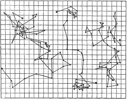
Figure 1: Three random trajectories of small mastic grains in water recorded by J. Perrin at 30-second intervals (reproduced from Perrin1909 ).

II.2 Mathematical view: multiscale construction

We start with the position “records” at every unit time: $t=1,2,3,...$ (e.g., every second) along one coordinate (two- and higher dimensional Brownian motion is then obtained by taking $d$ independent copies of the one-dimensional process). We focus on the time interval between $0$ and $1$, the construction being applicable to any interval $[\ell,\ell+1]$. For convenience, Brownian motion is started at $t=0$ from the origin: $B(0)=0$. By definition (or as a consequence of the central limit theorem if one relies on the above physical reasoning), the position at time $t=1$, $B(1)$, is a random variable $a_{0}$ distributed according to the standard normal (or Gaussian) law, ${\mathcal{N}}(0,1)$, with mean zero and variance one

$${\mathbb{P}}\{a_{0}\in(x,x+dx)\}=dx~{}\frac{e^{-x^{2}/2}}{\sqrt{2\pi}}.$$ (1)

In physics, the variance $\sigma^{2}$ is related to the diffusion coefficient, $D=\sigma^{2}/(2\tau)$, where $\tau$ is the one step duration; here, $\sigma=\tau=1$ yielding $D=1/2$ throughout the paper. A linear approximation at this time scale ($\delta=1$) is simply

$$B_{0}(t)=a_{0}t,$$

that connects the positions $B(0)=0$ and $B(1)=a_{0}$ by a linear segment.

If the time resolution is doubled, a new, intermediate position $b^{\prime}=B(1/2)$ can now be seen (Fig. 2). The random variable $b^{\prime}$ is conditioned by the fact that Brownian motion passes through the points $(0,0)$ and $(1,a_{0})$, the value of $a_{0}$ being already known. It is distributed according to the normal law with mean value $\frac{1}{2}(B(0)+B(1))=a_{0}/2$ and variance $1/4$ (see Appendix A). In other words, one can write $b^{\prime}=a_{0}/2+a_{00}/2$, where the new random variable $a_{00}\in{\mathcal{N}}(0,1)$ (i.e., distributed according to the standard normal law (1)) is independent of $B(0)=0$ and $B(1)=a_{0}$.

The linear approximation at the time scale $\delta=1/2$ connects three successive points $(0,0)$, $(1/2,b^{\prime})$ and $(1,a_{0})$ by two linear segments:

$$B_{1}(t)=\begin{cases}2tb^{\prime},\hskip 93.89409pt0\leq t\leq\frac{1}{2},\\ 2t(a_{0}-b^{\prime})+(2b^{\prime}-a_{0}),\quad\frac{1}{2}\leq t\leq 1.\end{cases}$$ (2)

The shape of this approximation looks like a skewed tent (Fig. 2) that can be represented as a sum of a linear shift and a “symmetric tent” function:

$$B_{1}(t)=a_{0}t+(2b^{\prime}-a_{0})h_{00}(t)=a_{0}t+a_{00}h_{00}(t),$$ (3)

where the “symmetric tent” function $h_{00}(t)$ is

$$h_{00}(t)=\begin{cases}t,\hskip 36.98857pt0\leq t\leq\frac{1}{2},\\ 1-t,\qquad\frac{1}{2}\leq t\leq 1,\\ 0,\hskip 36.98857pt\textrm{otherwise}.\end{cases}$$ (4)

The decomposition (3) into the linear function $t$ and the tent function $h_{00}(t)$ is unique. The new approximation $B_{1}(t)$ is obtained from the previous one, $B_{0}(t)$, by adding the new term representing a smaller geometrical detail.

Figure 2: Iterative construction of Brownian motion: (a) linear approximation $B_{0}(t)$ by a segment at scale $2^{0}$; (b) linear approximation $B_{1}(t)$ by two segments at scale $2^{-1}$. The latter “skewed tent” can be uniquely represented as the sum of a “symmetric tent” and a linear shift.

The same concept is applicable at every scale. Assume that an approximation $B_{n}(t)$ of Brownian motion is already constructed at the time scale $\delta=2^{-n}$, i.e., the positions $b_{k}=B(t_{k})$ are known at successive times $t_{k}=k2^{-n}$, $k$ ranging from $0$ to $2^{n}$. The approximate Brownian path is a piecewise linear function passing successively through these points.

At the next time scale $2^{-n-1}$, a new, intermediate position $b^{\prime}=B(t^{\prime})$ of Brownian motion at time $t^{\prime}=(t_{k}+t_{k+1})/2=(k+1/2)2^{-n}$ should be determined for each $k$. As previously, the random variable $b^{\prime}$ is conditioned by the fact that Brownian motion is known to pass through the points $(t_{k},b_{k})$ and $(t_{k+1},b_{k+1})$. It is again distributed according to the normal law, with mean value $(b_{k}+b_{k+1})/2$ and variance $2^{-n}/4$. In other words, one can write $b^{\prime}$ as

$$b^{\prime}=\frac{1}{2}(b_{k}+b_{k+1})+2^{-n/2-1}a_{nk},$$ (5)

where the new normal random variable $a_{nk}\in{\mathcal{N}}(0,1)$ is independent of the other positions. The linear segment between $(t_{k},b_{k})$ and $(t_{k+1},b_{k+1})$ is then replaced by two linear segments connecting the three successive points $(t_{k},b_{k})$, $(t^{\prime},b^{\prime})$, and $(t_{k+1},b_{k+1})$. This is a new “skewed tent” function which can be uniquely decomposed as the sum of the previous linear segment (drift) and a symmetric tent function $h_{nk}(t)$ with the weight $a_{nk}$, where

$$h_{nk}(t)=2^{-n/2}h_{00}(2^{n}t-k)$$ (6)

is a rescaled symmetric tent function on the interval $I_{nk}=[k2^{-n},(k+1)2^{-n})$ (see Fig. 3a). We stress again that the new approximation is obtained from the previous one by simply adding the tent function $h_{nk}(t)$, representing a smaller geometrical detail at the new scale $2^{-n-1}$, weighted by a normally distributed coefficient $a_{nk}$ which is independent of the previously determined positions.

Figure 3: Tent function $h_{nk}(t)$ (a) and the related Haar function $H_{nk}(t)$ (b), both having the support on the interval $I_{nk}=[k2^{-n},(k+1)2^{-n})$.

This construction is applicable to all linear segments (all $k$) at the given scale $n$, and it is valid for any scale. Repeating this procedure from the scale $2^{0}$ up to infinity, one obtains the Haar wavelet representation of Brownian motion on the unit interval:

$$B^{\omega}(t)=a_{0}^{\omega}t+\sum\limits_{n=0}^{\infty}\sum\limits_{k=0}^{2^{n}-1}a_{nk}^{\omega}h_{nk}(t),$$ (7)

where all weights $a_{0}^{\omega}$ and $a_{nk}^{\omega}$ are independent ${\mathcal{N}}(0,1)$ random variables. Here we introduced the superscript $\omega$ in order to stress that a sampling of Gaussian weights $a_{nk}$ yields a random realization of Brownian motion. We will discuss in Sect. II.4 that all these Gaussian weights can be constructed from a single random number $\omega$ from the unit interval that provides a natural parameterization of Brownian paths.

The dyadic structure of the intervals implies that for any $n\in{\mathbb{Z}}$, there exists only one interval $I_{nk}$ of length $2^{-n}$ containing the point $t$: $k2^{-n}\leq t<(k+1)2^{-n}$. The index $k$ is simply the integer part of $2^{n}t$: $k=\lfloor 2^{n}t\rfloor$ (i.e., the largest integer that does not exceed $2^{n}t$). As a consequence, the convergence in the above formula is very rapid. In fact, if one needs to obtain the value of function $B^{\omega}(t)$ with a desired precision $\varepsilon$, it is sufficient to calculate the first $\log_{2}(1/\varepsilon)$ terms, $\log_{2}x$ being the logarithm of $x$ on the base of $2$.

Subtracting the linear term $a_{0}^{\omega}t$ from Eq. (7) yields the Haar wavelet representation of a Brownian bridge on the unit interval, i.e., Brownian motion conditioned to return to $0$ at time $t=1$.

II.3 Dyadic decomposition and interval subdivision

In the wavelet representation (7), the first sum is carried over all scales $n$, while the second sum covers all $2^{n}$ subintervals $I_{nk}$ at the scale $n$. In some cases, it is convenient to enumerate all the dyadic subintervals $I_{nk}$ by a single index $m=2^{n}+k$ as shown on Fig. 4. Since $k$ is ranging from $0$ to $2^{n-1}$, the new index $m$ uniquely identifies the interval $I_{nk}$. In particular, one easily retrieves the pair $(n,k)$ from $m$ as

$$n=\lfloor\log_{2}m\rfloor,\hskip 28.45274ptk=m-2^{n}.$$

Using the notations

$$\tilde{a}_{m}^{\omega}=\begin{cases}~{}a_{0}^{\omega},\hskip 8.53581ptm=0,\\ a_{nk}^{\omega},~{}~{}m>0,\\ \end{cases}\hskip 14.22636pt\tilde{h}_{m}(t)=\begin{cases}~{}~{}~{}t,\hskip 19.91692ptm=0,\\ h_{nk}(t),~{}~{}m>0,\\ \end{cases}$$

we can write Eq. (7) in a more compact form

$$B^{\omega}(t)=\sum\limits_{m=0}^{\infty}\tilde{a}_{m}^{\omega}~{}\tilde{h}_{m}(t).$$ (8)

As a result, Brownian trajectory is decomposed into a sum of tent functions (plus a linear drift) with random independent identically distributed Gaussian weights. As illustrated below, all these weights can be determined from a single uniformly distributed random variable.

Figure 4: Enumeration of the dyadic subintervals by a single index $m$.

II.4 Representation of Gaussian weights

In this subsection, we illustrate how all random Gaussian weights $\tilde{a}^{\omega}_{m}$ can be explicitly related to a single uniformly distributed random number $\omega$. In other words, we show that the complicated abstract probability space of Brownian paths can have a simple parameterization. However, this construction is not relevant from practical point of view, and the subsection can be skipped at first reading.

We consider the binary expansion of a given real number $\omega$ from the unit interval

$$\omega=0.b_{1}b_{2}b_{3}b_{4}\ldots$$ (9)

where $b_{i}$ are equal to $0$ or $1$ (note that $\omega=1$ is expanded as $0.111\ldots$ instead of its equivalent form $1.000\ldots$). A uniform picking up of $\omega$ in $[0,1]$ is equivalent to independent random choice of its binary digits (or bits) $b_{i}$. Then we choose a prime number $p$ and construct another number $\omega_{p}$ using the bits of $\omega$ at positions $p$, $p^{2}$, $p^{3}$, $\ldots$

$$\omega_{p}=0.b_{p}b_{p^{2}}b_{p^{3}}b_{p^{4}}\ldots$$ (10)

For example, $\omega_{2}=0.b_{2}b_{4}b_{8}b_{16}\ldots$, $\omega_{3}=0.b_{3}b_{9}b_{27}b_{81}\ldots$, etc. (Fig. 5). If $p$ and $q$ are two different prime numbers then $\omega_{p}$ and $\omega_{q}$ are independent as being constructed from separate sets of independent bits $b_{i}$. Moreover, if $\omega$ is chosen uniformly from the unit interval, then each $\omega_{p}$ is also uniformly distributed on the unit interval. Consequently, a single random number $\omega$ gives rise to an infinite sequence $\{\omega_{p}\}$ of independent uniformly distributed random variables. In a more formal way, the real numbers $\omega_{p}$ can be written as

$$\omega_{p}=\sum\limits_{n=1}^{\infty}2^{-n-1}\bigl{(}1+R(2^{p^{n}}\omega)\bigr{)},$$ (11)

where $R(x)=(-1)^{\lfloor x\rfloor}$ is the Rademacher function.

Figure 5: Generation of an infinite sequence of independent uniformly distributed variables $\omega_{2}$, $\omega_{3}$, $\omega_{5}$, $\ldots$ using binary expansion of a single number $\omega$ from the unit interval. For instance, $\omega_{2}$ is constituted of the $2^{\rm nd}$, $4^{\rm th}$, $8^{\rm th}$, $\ldots$ bits of $\omega$.

At last, we need to pass from uniformly distributed to normally distributed variables. For this purpose, we define the inverse $\Phi(x)$ of the error function: for $x\in[0,1]$, the value $y$ of the function $\Phi(x)$ satisfies

$$\frac{1}{\sqrt{2\pi}}\int\limits_{-\infty}^{y}dz~{}e^{-z^{2}/2}=x.$$ (12)

Although there is no simple analytic form for the function $\Phi(x)$, many properties can be easily derived, and the whole function can be tabulated with any required precision.

If $p_{m}$ denotes the $(m+1)^{\rm th}$ prime (e.g., $p_{0}=2$, $p_{1}=3$, $p_{2}=5$), then we set

$$\tilde{a}_{m}^{\omega}=\Phi(\omega_{p_{m}}),\hskip 22.76219ptm=0,1,2,...$$ (13)

By construction, $\tilde{a}_{m}^{\omega}$ are independent normally distributed random variables. In other words, Eqs. (11, 12) map a uniformly distributed $\omega$ onto a sequence of Gaussian weights $\tilde{a}_{m}$. As a result, $B^{\omega}(t)$ is constructed as a mapping from the unit interval, $\omega\in[0,1]$, onto the space of real-valued functions (more precisely, the Hölder space $H_{1/2-\epsilon}$ with any $\varepsilon>0$). In other words, any Brownian path is explicitly encoded by the real number $\omega$. Picking up the real number $\omega$ from the unit interval (with uniform measure) is thus equivalent to choosing a Brownian path (with Wiener measure). In this representation, the probability space for Brownian motion is nothing else than the unit interval with uniform measure. It is intuitively much simpler than the classical construction of the probability space by means of Wiener measure, filtrations, etc. At the same time, this mapping is evidently neither continuous, nor injective (e.g., two numbers $\omega$ and $\omega^{\prime}$ that differ at 6-th bit correspond to the same sequence of Gaussian random numbers). The mapping remains a rather formal construction whose only purpose was to show the equivalence between two spaces.

II.5 Haar wavelets

In Eqs. (7) or (8), Brownian motion is decomposed into a sum of a linear function and tent functions. Figure 3a illustrates that any tent function $h_{nk}(t)$ can actually be represented as the integral of a piecewise-constant function

$$h_{nk}(t)=\int\limits_{0}^{t}dt^{\prime}~{}H_{nk}(t^{\prime}),$$ (14)

where $H_{nk}(t)$ is called the Haar function and defined to be $0$ on the complement of $I_{nk}$ and to take values $2^{n/2}$ and $-2^{n/2}$ on its left and right subintervals, respectively (Fig. 3b). In fact, all Haar functions are obtained by translations and dilations of a single “mother” function $\phi^{1,1}(t)$:

$$\phi^{1,1}(t)=\begin{cases}~{}~{}1,~{}~{}~{}~{}0\leq t<\frac{1}{2},\\ -1,\quad\frac{1}{2}<t\leq 1,\\ ~{}~{}0,~{}~{}~{}~{}\textrm{otherwise}.\\ \end{cases}$$ (15)

As illustrated on Fig. 6, one has

$$H_{nk}(t)=2^{n/2}\phi^{1,1}(2^{n}t-k).$$ (16)

It is convenient to use previously introduced single index $m$ to denote different Haar functions:

$$\tilde{H}_{m}(t)=\begin{cases}~{}~{}1,\hskip 22.76219ptm=0,\\ H_{nk}(t),~{}~{}m>0.\\ \end{cases}$$

Eq. (8) yields the following representation for Brownian motion

$$B^{\omega}(t)=\int\limits_{0}^{t}dW^{\omega}(t^{\prime}),$$ (17)

where $dW^{\omega}(t)$ denotes the Gaussian white noise which is defined here through the Haar wavelet decomposition

$$dW^{\omega}(t)=\sum\limits_{m=0}^{\infty}\tilde{a}_{m}^{\omega}~{}\tilde{H}_{m}(t).$$ (18)

Figure 6: Haar wavelets $H_{nk}(t)$ are obtained by dilations and translations of the mother function $\phi^{1,1}(t)=H_{00}(t)$ (shown on the left).

It is easy to check that Haar functions $\{\tilde{H}_{m}(t)\}$ (together with a constant function) form an orthonormal basis in the space $L^{2}([0,1])$ of measurable and square integrable functions that is

$$\int\limits_{0}^{1}dt~{}\tilde{H}_{m}(t)\tilde{H}_{m^{\prime}}(t)=\delta_{m,m^{\prime}}.$$

Moreover, this basis is known to be complete in $L^{2}([0,1])$. This means that any function from $L^{2}([0,1])$ can be decomposed into a linear combination of the Haar functions (and a constant). From now on, we drop the superscript $\omega$ for getting simpler notations although the parameterization by $\omega$ remains valid for all discussed processes.

II.6 General spectral representation

The wavelet representation (18) can be extended to any complete orthonormal basis $\{\psi_{i}(t)\}$ of $L^{2}([0,1])$. In fact, if the orthonormal basis $\{\psi_{i}(t)\}$ is complete, one can decompose any function $\tilde{H}_{m}(t)$ into a linear combination of $\psi_{i}(t)$:

$$\tilde{H}_{m}(t)=\sum\limits_{i=0}^{\infty}c_{m,i}~{}\psi_{i}(t),$$

where the coefficients $c_{m,i}$ satisfy the orthogonality relation

$$\sum\limits_{m=0}^{\infty}c_{m,i}^{2}=1\qquad(i=0,1,2,\ldots).$$ (19)

Substitution of this decomposition into Eq. (18) gives

$$dW(t)=\sum\limits_{m=0}^{\infty}\tilde{a}_{m}\sum\limits_{i=0}^{\infty}c_{m,i}~{}\psi_{i}(t)=\sum\limits_{i=0}^{\infty}\hat{a}_{i}~{}\psi_{i}(t),$$ (20)

with new random weights

$$\hat{a}_{i}=\sum\limits_{m=0}^{\infty}\tilde{a}_{m}~{}c_{m,i}.$$

The sum of independent Gaussian variables is a Gaussian variable, and its variance is simply the sum of the squared coefficients $c_{m,i}^{2}$, which is equal to $1$ according to Eq. (19). In other words, $\hat{a}_{i}\in{\mathcal{N}}(0,1)$. Moreover, the new random variables $\hat{a}_{i}$ are independent due to the orthogonality of the functions $\psi_{i}(t)$. We have thus shown that the Gaussian white noise can be decomposed into a linear combination with independent Gaussian weights in arbitrary complete orthonormal basis of $L^{2}([0,1])$.

The completeness of the basis $\{\psi_{i}(t)\}$ yields the usual covariance of the Gaussian white noise

$$\begin{split}{\mathbb{E}}\{dW(t_{1})dW(t_{2})\}&=\sum\limits_{i_{1},i_{2}=0}^{\infty}\psi_{i_{1}}(t_{1})\psi_{i_{2}}(t_{2}){\mathbb{E}}\{\hat{a}_{i_{1}}\hat{a}_{i_{2}}\}\\ &=\sum\limits_{i=0}^{\infty}\psi_{i}(t_{1})\psi_{i}(t_{2})=\delta(t_{1}-t_{2}),\\ \end{split}$$

where $\delta$ is the Dirac distribution (or “$\delta$-function”).

Substituting Eq. (20) into Eq. (17), one gets

$$B(t)=\sum\limits_{i=0}^{\infty}\hat{a}_{i}\int\limits_{0}^{t}dt^{\prime}~{}\psi_{i}(t^{\prime}),$$ (21)

For instance, one can consider the Fourier basis on the unit interval,

$$\psi_{i}(t)=\sqrt{2}~{}\cos(\pi(i-1/2)t),$$

in order to get the Karhunen-Loève expansion of Brownian motion Loeve :

$$B(t)=\sqrt{2}\sum\limits_{i=0}^{\infty}\hat{a}_{i}~{}\frac{\sin(\pi(i-1/2)t)}{(i-1/2)\pi}.$$ (22)

II.7 Basic properties of Brownian motion

We have explicitly constructed the Haar wavelet decomposition (7) and then general representation (21) in order to reproduce the basic properties of Brownian motion. Alternatively, one could first postulate such a representation as a definition of Brownian motion and then check that the basic properties are fulfilled. To illustrate this point, we check several properties.

(i) Brownian motion is a Gaussian process with independent increments. First, $B(t)$ is Gaussian as being a linear combination (21) of Gaussian variables. Let $t_{1}<t_{2}$ and $t_{3}<t_{4}$ define two increments, $B(t_{2})-B(t_{1})$ and $B(t_{4})-B(t_{3})$. If $t_{2}\leq t_{3}$ (i.e., the increments do not “overlay”), then they are independent (similar statement holds if $t_{4}\leq t_{1}$ by symmetry). To proof this statement, we decompose the unit interval as

$$[0,1]=[0,t_{1})\cup[t_{1},t_{2}]\cup(t_{2},t_{3})\cup[t_{3},t_{4}]\cup(t_{4},1],$$ (23)

(if one of subintervals $[0,t_{1})$, $(t_{2},t_{3})$ or $(t_{4},1]$ is empty, it can be ignored). The basis $\{\psi_{i}(t)\}$ in Eq. (21) can be chosen as the direct product of the Haar eigenbases on each subinterval. For instance, $\{\psi_{i}^{[t_{1},t_{2}]}\}$ is the Haar basis of $L^{2}([t_{1},t_{2}])$ which is extended to $[0,1]\backslash[t_{1},t_{2}]$ by zeros. In this particular representation, one has

$$\begin{split}&B(t_{2})-B(t_{1})=\int\limits_{t_{1}}^{t_{2}}dt^{\prime}\sum\limits_{i=0}^{\infty}\hat{a}_{i}~{}\psi_{i}(t^{\prime})\\ &=\int\limits_{t_{1}}^{t_{2}}dt^{\prime}\sum\limits_{i=0}^{\infty}\hat{a}_{i}^{[t_{1},t_{2}]}~{}\psi_{i}^{[t_{1},t_{2}]}(t^{\prime})=\hat{a}_{0}^{[t_{1},t_{2}]}~{}\sqrt{t_{2}-t_{1}}.\\ \end{split}$$ (24)

In the second equality, the Haar functions from other subintervals (except $[t_{1},t_{2}]$) vanished by construction. In turn, all the Haar functions $\psi_{i}^{[t_{1},t_{2}]}(t^{\prime})$ on $[t_{1},t_{2}]$ (with $i>0$) vanished after integration due to their orthogonality to the constant. The only remaining contribution is the constant term which has the unit $L^{2}([t_{1},t_{2}])$ norm: $\psi_{0}^{[t_{1},t_{2}]}(t)=(t_{2}-t_{1})^{-1/2}$. Integrating this term, one gets the right-hand side of Eq. (24) which shows that the increment $B(t_{2})-B(t_{1})$ is a Gaussian variable with mean zero and variance $t_{2}-t_{1}$, as expected. Moreover, the same representation for $[t_{3},t_{4}]$ yields

$$\begin{split}&B(t_{4})-B(t_{3})=\int\limits_{t_{3}}^{t_{4}}dt^{\prime}\sum\limits_{i=0}^{\infty}\hat{a}_{i}~{}\psi_{i}(t^{\prime})\\ &=\int\limits_{t_{3}}^{t_{4}}dt^{\prime}\sum\limits_{i=0}^{\infty}\hat{a}_{i}^{[t_{3},t_{4}]}~{}\psi_{i}^{[t_{3},t_{4}]}(t^{\prime})=\hat{a}_{0}^{[t_{3},t_{4}]}~{}\sqrt{t_{3}-t_{4}},\\ \end{split}$$ (25)

and the random weights $\hat{a}_{0}^{[t_{1},t_{2}]}$ and $\hat{a}_{0}^{[t_{3},t_{4}]}$ are independent by construction. As a consequence, the increments $B(t_{2})-B(t_{1})$ and $B(t_{4})-B(t_{3})$ are independent.

(ii) The mean and covariance of Brownian motion are:

$${\mathbb{E}}\{B(t)\}=0,\qquad{\mathbb{E}}\{B(t_{1})B(t_{2})\}=\min\{t_{1},t_{2}\}.$$ (26)

The first statement is obvious from Eq. (21) given that all weights have mean zero. To prove the second statement, one assumes that $t_{2}>t_{1}$ and considers

$$\begin{split}{\mathbb{E}}\{B(t_{1})B(t_{2})\}&={\mathbb{E}}\{(B(t_{1})-B(0))(B(t_{2})-B(t_{1})\}\\ &+{\mathbb{E}}\{[B(t_{1})-B(0)]^{2}\}.\\ \end{split}$$

The first term vanishes due to the independence of increments (and $B(0)=0$), while the second term is equal to $t_{1}$ according to Eq. (24).

(iii) Brownian motion is continuous but nowhere differentiable almost surely. The proof relies on a simple fact that the Gaussian weights $a_{nk}$ cannot be too large, e.g., the probability that $|a_{nk}|>n$ decays extremely fast (as $e^{-n^{2}/2}$ for large enough $n$). In turn, the norm of tent functions decreases exponentially that ensures the continuity of Brownian motion and the convergence of a partial sum approximation in Eq. (7) or similar expressions to Brownian motion. Moreover, the remainder of this approximation decreases exponentially fast with the truncated scale $N$ (for technical details, see Appendix B).

II.8 Alpert-Rokhlin wavelets

As we mentioned in Sect. II.1, taking the particular orthonormal basis is equivalent to choosing a way to connect successive positions of Brownian motion at a finite scale $\delta$. The Haar wavelets and the resulting tent functions present the simplest way of connection by linear segments. Such a piecewise linear approximation of Brownian motion introduces singularities at the connection nodes (corners). For some problems, it is convenient to deal with a smooth approximation of Brownian motion at finite scales (although a true Brownian trajectory, the limiting curve, remains nowhere differentiable). For this purpose, one can use the Alpert-Rokhlin multiwavelet basis Alpert ; Alpert92 ; Beylkin91 ; Beylkin92 . This basis is generated by a set of $q$ functions $\phi^{q,1}(t),\ldots,\phi^{q,q}(t)$ which are supported on the interval $[0,1]$, are piecewise polynomials of degree $q-1$ on $[0,1/2]$ and on $[1/2,1]$, and satisfy the moment cancellation conditions

$$\int\limits_{0}^{1}dt~{}t^{k}~{}\phi^{q,p}(t)=0,~{}~{}~{}\begin{array}[]{l}k=0,1,\ldots,q-1,\\ p=1,2,\ldots,q.\\ \end{array}$$ (27)

These mother functions generate the Alpert-Rokhkin multiwavelets of order $q$ by translations and dilations:

$$\phi^{q,p}_{nk}(t)=2^{-n/2}\phi^{q,p}(2^{n}t-k)\qquad\begin{array}[]{l}n=0,1,2,\ldots,\\ k=0,1,2,\ldots 2^{n}-1.\\ \end{array}$$

The set of functions $\{\phi^{q,p}_{nk}(t)\}$, completed by the set of orthonormal polynomials of order $m<q$, forms a complete basis of $L^{2}([0,1])$. This completion is necessary because all mother functions $\phi^{q,p}(t)$ (and thus all $\phi^{q,p}_{nk}(t)$) are orthogonal by construction to all polynomials of order $m<q$. Similarly, the Haar wavelets were completed by a constant function.

When $q=1$, there is only one mother function $\phi^{1,1}(t)$ defined by Eq. (15) which generates the Haar wavelets by translations and dilations. For $q=2$, there are two mother functions (Fig. 7), satisfying the moment cancellation conditions (27):

$$\begin{split}\phi^{2,1}(t)&=\begin{cases}\sqrt{3}~{}(1-4t),\qquad 0\leq t<\frac{1}{2},\\ \sqrt{3}~{}(4t-3),\qquad\frac{1}{2}<t\leq 1,\\ ~{}~{}~{}~{}~{}~{}~{}0,\hskip 42.67912pt\textrm{otherwise}\\ \end{cases}\\ \phi^{2,2}(t)&=\begin{cases}6t-1,\qquad 0\leq t<\frac{1}{2},\\ 6t-5,\qquad\frac{1}{2}<t\leq 1,\\ ~{}~{}~{}~{}0,\hskip 28.45274pt\textrm{otherwise}\\ \end{cases}\\ \end{split}$$

Higher-order mother functions (with $q>2$) can be constructed through an orthogonalization procedure (see Alpert ; Elliott94 for details and examples).

Note that the wavelet representation of Brownian motion involves the integral of wavelets

$$h^{q,p}_{00}(t)=\int\limits_{0}^{t}dt^{\prime}\phi^{q,p}(t^{\prime}).$$ (28)

For instance, one gets for $q=2$ (Fig. 7)

$$h^{2,1}_{00}(t) = \begin{cases}\sqrt{3}~{}t~{}(1-2t),\hskip 34.1433pt0\leq t<\frac{1}{2},\\ \sqrt{3}~{}(1-t)(1-2t),\quad\frac{1}{2}<t\leq 1,\\ \end{cases}$$

$$h^{2,2}_{00}(t) = \begin{cases}t~{}(3t-1),\hskip 34.1433pt0\leq t<\frac{1}{2},\\ (t-1)(3t-2),\quad\frac{1}{2}<t\leq 1.\\ \end{cases}$$

while the other functions $h^{2,1}_{nk}(t)$ and $h^{2,2}_{nk}(t)$ are obtained by dilations and translations. As a consequence, Brownian motion gets a closed formula in terms of the Alpert-Rohklin multiwavelets of order $2$:

$$B(t)=a_{0}t+a_{1}\sqrt{3}t(t-1)+\sum\limits_{n=0}^{\infty}\sum\limits_{k=0}^{2^{n}-1}\sum\limits_{p=1}^{2}a_{nk}^{(p)}h^{2,p}_{nk}(t),$$ (29)

where all weights $a_{0}$, $a_{1}$, $a_{nk}^{(p)}$ are independent ${\mathcal{N}}(0,1)$ variables, and the second term is the integral of the linear basis function $\sqrt{3}(2t-1)$. An extension of this representation to the Alpert-Rohklin multiwavelet basis of order $q$ is straightforward.

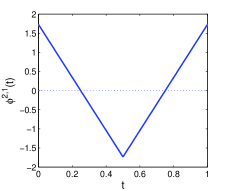
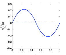
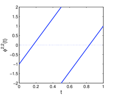
Figure 7: Two mother functions for Alpert-Rokhlin first-order multiwavelets (on the left) and their integrals $h^{q,p}_{00}(t)$ (on the right). The use of these wavelets corresponds to another type of connection (not by linear segments) between successive points of Brownian motion in the refinement procedure. For comparison, the tent function $h_{00}(t)$ is shown on the last plot by dashed line. Note that horizontal and vertical scales are not matched here.

II.9 Numerical implementation

The wavelet representation of Brownian motion can be easily implemented in practice. To carry computations with a (fixed) desired precision $\varepsilon$, it is sufficient to truncate the first sum in Eq. (7) or equivalent relation up to $N=\lfloor\log_{2}(1/\varepsilon)\rfloor$, because higher-order terms describe geometrical details at smaller scales. The remainder of this series can be estimated using Eq. (49). For Haar wavelets, such a truncation qualitatively corresponds to an approximation of Brownian motion by a broken line composed of linear segments of length close to $\varepsilon$, while the Alpert-Rokhlin wavelets yield smoother approximations (Fig. 8). This is a fascinating feature of wavelets, allowing one to capture geometrical details at different scales.

A realization of a Brownian path is completely determined by a set of random coefficients $a_{nk}^{\omega}$ (or $\tilde{a}_{m}^{\omega}$). In Sect. II.4, we discussed an explicit scheme to generate all these coefficients from a randomly chosen number $\omega$ from the unit interval. In practice, one can use standard routines to generate pseudo-random normally distributed weights $a_{nk}^{\omega}$ (or $\tilde{a}_{m}^{\omega}$). The computation of tent functions $h_{nk}(t)$ can be easily implemented. Consequently, the computation of $B(t)$ at any time $t$ requires only $\log_{2}(1/\varepsilon)$ operations, each of them consisting of finding $h_{nk}(t)$, multiplying it by $a_{nk}^{\omega}$, and summing their contributions.

Figure 8: A random Brownian path at scales $n=3$ (dashed line), and $n=10$ (solid line) with Haar wavelets (a) and Alpert-Rohkin wavelets with $q=2$ (b).

It is instructive to compare the wavelet approach to conventional techniques. We consider the computation of all positions $b_{k}=B(t_{k})$ at equidistant times $t_{k}=k2^{-N}$ ($k=0,...,2^{N}$) at some scale $\varepsilon=2^{-N}$. In a classical scheme, Brownian motion is modeled by a sequence of small random jumps

$$b_{0}=0,\hskip 28.45274ptb_{k+1}=b_{k}+2^{-N/2}a^{\prime}_{k}~{}~{}~{}(k=0,1,...,2^{N}-1),$$ (30)

with $2^{N}$ independent normally distributed random variables $a^{\prime}_{k}\in{\mathcal{N}}(0,1)$. Similar computation relying on wavelet representations requires one random variable for a linear shift and $2^{k}$ random variables at each scale $k$, $k$ ranging from $0$ to $N-1$. The total number is then $1+(1+2+4+...+2^{N-1})=2^{N}$. It is not surprising that both schemes require the same degree of randomness to represent a Brownian path at chosen scale. The wavelet representation does not reduce the complexity or randomness, but re-organize the data in a hierarchical structure to facilitate their use. For instance, formula (7) accesses approximate positions of Brownian motion at any time point $t$, not necessarily $t_{k}$. In a classical scheme, one could use a linear interpolation between two neighboring points to get the same result. Again, the wavelets do not bring new features which are not available by conventional techniques, but provide another, structured and efficient, representation.

Throughout the above sections, Brownian motion was constructed on the unit interval for convenience. The constructed process can be easily rescaled to any finite interval, while an extension to ${\mathbb{R}}_{+}$ or ${\mathbb{R}}$ is possible as well. Finally, an extension to isotropic Brownian motion in ${\mathbb{R}}^{d}$ is obtained by taking $d$ independent samples of one-dimensional Brownian motion.

III Beyond Brownian motion

III.1 Fractional Brownian motion

A similar technique can be applied to construct and study fractional Brownian motion which is also known as random fractal velocity field Kolmogorov40 ; Mandelbrot68 . For instance, random fractal velocity field with the Hurst exponent $H=1/3$ (defined below) corresponds to the Kolmogorov spectrum in high Reynolds number turbulence Mandelbrot ; Lesieur ; McComb ; Majda99 . Fractional Brownian motion, as a Gaussian stochastic process with long-range correlations, has found numerous applications in different fields, ranging from transport phenomena in porous media Elliott94 ; Elliott95 ; Elliott95b ; Elliott97 ; Bunde to analysis of financial markets Mandelbrot97 .

P. Lévy proposed the first extension of Eq. (17) by using the Riemann-Liouville fractional integration which can be thought of as a moving average of a Gaussian white noise Levy53

$$\tilde{B}_{H}(t)=\frac{1}{\Gamma(H+\frac{1}{2})}\int\limits_{0}^{t}(t-s)^{H-\frac{1}{2}}dW(s),$$ (31)

where $0<H<1$ is the Hurst exponent, and $\Gamma(H+1/2)$ is the normalization factor ($\Gamma(z)$ being the Gamma function). Mandelbrot and van Ness discussed the limitations of this definition (e.g., its strong emphasis on the origin) and proposed to use the Weyl fractional integral that yields Mandelbrot68

$$\begin{split}B_{H}(t)&=\frac{1}{\Gamma(H+\frac{1}{2})}\biggl{\{}\int\limits_{-\infty}^{0}\bigl{[}(t-s)^{H-\frac{1}{2}}-(-s)^{H-\frac{1}{2}}\bigr{]}dW(s)\\ &+\int\limits_{0}^{t}(t-s)^{H-\frac{1}{2}}dW(s)\biggr{\}}\\ \end{split}$$ (32)

for $t>0$ (and similar for $t<0$). The last representation can also be written as (see Decreusefond99 )

$$B_{H}(t)=\int\limits_{0}^{t}K_{H}(t,s)~{}dW(s),$$ (33)

where

$$K_{H}(t,s)=\frac{(t-s)^{H-\frac{1}{2}}}{\Gamma(H+\frac{1}{2})}~{}_{2}F_{1}\biggl{(}H-\frac{1}{2},\frac{1}{2}-H;H+\frac{1}{2};1-\frac{t}{s}\biggr{)},$$ (34)

and ${}_{2}F_{1}(a,b;c;z)$ is the hypergeometric function. The ordinary Brownian motion is retrieved at $H=1/2$ for all cases.

Using a wavelet representation (20) for the Gaussian white noise, one obtains

$$B_{H}(t)=\sum\limits_{i=0}^{\infty}\hat{a}_{i}\int\limits_{0}^{t}ds~{}K_{H}(t,s)\psi_{i}(s).$$ (35)

The integrals can be evaluated using an appropriate basis $\{\psi_{i}(t)\}$. Moreover, the moment cancellation property (27) for the Alpert-Rokhlin multiwavelets with a large enough order $q$ guarantees that the integrals in Eq. (35) are highly localized, yielding a rapid convergence of the above sum. This convergence is a key point for efficient numerical algorithms for simulation of fractional Brownian motion (see Elliott94 ; Elliott95 ; Elliott95b ; Elliott97 ). Among other numerical methods, we mention alternative wavelet representations Wornell90 ; Flandrin92 ; Sellan95 ; Arby96 (e.g., the method by Arby and Sellan is implemented in the Matlab function ‘wfmb’), circulant embedding of the covariance matrix Davies87 ; Wood94 ; Dietrich97 , and random midpoint displacement method Fournier82 which is often used in computer graphics to generate random two-dimensional landscapes.

In general, the kernel $K_{H}(t,t^{\prime})$ can be replaced by any convenient kernel to extend this approach to various Gaussian processes. For instance, setting $K(t,t^{\prime})=e^{-\theta(t-t^{\prime})}$ yields the Ornstein-Uhlenbeck process Uhlenbeck30 ; Risken . Similarly, one can deal with various stochastic dynamics generated by Langevin equations Coffey .

III.2 Gaussian Free Field and its extensions

Brownian motion is the integral of the Gaussian white noise which, in turn, is obtained as a linear combination of orthonormal functions $\{\psi_{i}\}$ forming a complete basis of the space $L^{2}([0,1])$, with standard Gaussian weights. This construction can be extended to any separable Hilbert space $H$. However, whatever the functional space $H$ is taken, a linear combination of its orthonormal basis functions with standard Gaussian weights does not belong to this space (the argument is the same as for $L^{2}$ space, the norm of such a linear combination being infinite). In particular, the Gaussian white noise is not a function but a distribution. In order to construct extensions of the Gaussian white noise with desired properties, one needs to carefully choose the Hilbert space $H$. In this section, we briefly discuss two such extensions: Gaussian free field (GFF) Sheffield07 and fractional Gaussian field (FGF) with logarithmic correlations Lodhia14 ; Duplantier14 . The GFF appears as the basic description of massless non-interacting particles in field theories. Both GFF and FGF constitute important models in different areas of physics, from astrophysics (describing stochastic anisotropy in cosmic microwave background) to critical phenomena, quantum physics, and turbulence Bardeen86 ; Kobayashi11 ; Fernandez ; Dodelson . While the “sequence” of random variables of Brownian motion $B(t)$ was naturally parameterized by “time” $t$ (a real number from the unit interval or, in general, from ${\mathbb{R}}$), random variables of a field can in general be parameterized by points from an Euclidean domain, a manifold, or a graph. For instance, one can speak about random surfaces which can model landscapes (e.g., mountains) or ocean’s water surface, in which the height is parameterized by two coordinates. The geometrical structure of “smooth” random surfaces was thoroughly investigated Adler ; Adler2 ; Vanmarcke , especially for Gaussian fields which are fully characterized by their mean and covariance. Important examples of smooth Gaussian fields are the random plane waves and random spherical harmonics (see Berry77 ; Nazarov10 ). In turn, the GFF and FGF are examples of highly irregular random fields. As Brownian motion can be obtained as the limit of discrete random walks, the Gaussian free field in two dimensions appears in the limit of discrete random surfaces Kondev95 ; Schramm09 .

The Gaussian free field is constructed by choosing the Dirichlet Hilbert space $H_{\nabla}(\Omega)$, in which the scalar product of two functions $f$ and $g$ is defined as

$$\langle f,g\rangle_{H_{\nabla}(\Omega)}=\int\limits_{\Omega}dx~{}(\nabla f\cdot\nabla g)$$ (36)

for a given Euclidean domain $\Omega\subset{\mathbb{R}}^{d}$. When $\Omega$ is bounded, an orthonormal basis of this space can be obtained by setting $\psi_{i}(x)=\lambda_{i}^{-1/2}u_{i}(x)$, where $u_{i}(x)$ are the $L^{2}$-normalized Dirichlet eigenfunctions of the Laplace operator: $\Delta u_{i}(x)+\lambda_{i}u_{i}(x)=0$ in $\Omega$ with $u_{i}(x)=0$ at the boundary $\partial\Omega$, and $\lambda_{i}$ are the corresponding eigenvalues. The Gaussian free field on $\Omega$ is defined as

$$F(x)=\sum\limits_{i=0}^{\infty}a_{i}~{}\psi_{i}(x)$$ (37)

where $a_{i}\in{\mathcal{N}}(0,1)$ are independent Gaussian weights. Given that the eigenvalues $\lambda_{i}$ asymptotically grow as $i^{2/d}$ according to the Weyl’s law Courant ; Grebenkov13 , the sum in Eq. (37) is convergent for $d=1$ (in which case the GFF is simply a Brownian bridge) but diverges in higher dimensions. In the plane, this sum barely misses the convergence, being logarithmically diverging. In quantum field theory, it is related to the infra-red divergence for massless particles. As a consequence, $F(x)$ is not a function but a distribution for $d>1$. Being a linear combination of normal variables, the field $F(x)$ is Gaussian and thus is fully characterized by its mean ${\mathbb{E}}\{F(x)\}=0$ and the covariance

$${\mathbb{E}}\{F(x_{1})F(x_{2})\}=\sum\limits_{i=0}^{\infty}\lambda_{i}^{-1}u_{i}(x_{1})u_{i}(x_{2})=G(x_{1},x_{2}),$$ (38)

where the right-hand side can be recognized as the Green function $G(x_{1},x_{2})$ of the Laplace operator in the domain $\Omega$. Alternatively, one could define the GFF by setting the covariance equal to the Green function (in which case the definition holds even for unbounded domains). Strictly speaking, since the sum in Eq. (37) diverges for $d>1$, the GFF should be treated as a distribution by its action on every fixed test function $\phi(x)$. In particular, the covariance should be given by covariance of actions of $F$ on two test functions $\phi_{1}$ and $\phi_{2}$:

$${\mathbb{E}}\{F\phi(x_{1}),F\phi(x_{2})\}=\int\limits_{\Omega\times\Omega}dx_{1}dx_{2}~{}G(x_{1}-x_{2})~{}\phi_{1}(x_{1})~{}\phi_{2}(x_{2}).$$ (39)

The fractional Gaussian fields can be obtained by replacing the gradient operators $\nabla$ in the scalar product (36) by fractional Laplacians Chen10 ,

$$\langle f,g\rangle_{H_{\nabla}^{\nu}(\Omega)}=\int\limits_{\Omega}dx~{}((-\Delta)^{\nu}f\cdot(-\Delta)^{\nu}g),$$ (40)

for a positive $\nu$. The Dirichlet Hilbert space is retrieved for $\nu=1/2$. In a similar way, the functions $\psi_{i}(x)=\lambda_{i}^{-\nu/2}u_{i}(x)$ form a basis of the space $H_{\nabla}^{\nu}(\Omega)$, from which the FGF is constructed as in Eq. (37). This sum is convergent for $\nu>d/4$ and divergent otherwise. In the particular case $\nu=d/4$, the FGF is logarithmically divergent in all dimensions. Note that the FGF coincides with the GFF in the plane ($d=2$). In particular, the FGF with logarithmic correlations on the unit interval reads explicitly as

$$F(t)=\sqrt{\frac{2}{\pi}}\sum\limits_{k=1}^{\infty}a_{k}~{}\frac{\sin(\pi kt)}{\sqrt{k}}.$$ (41)

More generally, one can take any orthonormal basis $\{u_{i}(t)\}$ of $L^{2}([0,1])$ and then apply the operator $(-\Delta)^{-1/4}=\bigl{(}\frac{d}{dt}\bigr{)}^{-1/2}$ to get the basis of $H_{\nabla}^{1/4}([0,1])$. The advantage of the Laplacian eigenbasis is that the fractional integral operator $\bigl{(}\frac{d}{dt}\bigr{)}^{-1/2}$ (which can be defined through the Fourier transform) is replaced by multiplication by $\lambda_{i}^{-1/4}$. As a consequence, the FGF with logarithmic corrections in one dimension appears as the half-derivative of Brownian motion:

$$\begin{split}F(t)&=\sum\limits_{i=0}^{\infty}a_{i}\biggl{(}\frac{d}{dt}\biggr{)}^{-1/2}u_{i}(t)\\ &=\sum\limits_{i=0}^{\infty}a_{i}\biggl{(}\frac{d}{dt}\biggr{)}^{1/2}\int\limits_{0}^{t}dt^{\prime}~{}u_{i}(t^{\prime})=\biggl{(}\frac{d}{dt}\biggr{)}^{1/2}B(t).\\ \end{split}$$ (42)

This formula reveals a very close relation between these two processes which are often considered as distinct objects. Note that the series in Eq. (42) diverges logarithmically, while the derivative of order $1/2-\epsilon$ would lead to converging series. In other words, Brownian motion belongs to the Hölder space $H_{1/2-\epsilon}$ (for any $\epsilon>0$) so that its derivatives of order less than $1/2$ exist, but $1/2$ and higher do not. As for Brownian motion, the explicit closed formula (37) allows one to sample random realizations of the FGF by picking up $\omega$ from the unit interval, i.e., the probability space for this process is nothing else than the unit interval with uniform measure.

IV Restricted diffusion

In this section, we briefly discuss how multiscaling and dyadic decompositions help simulating restricted diffusion. This is an ubiquitous problem in physics (e.g., transport in porous media), chemistry (e.g., heterogeneous catalysis), biology and physiology (e.g., diffusion in cells, tissues, and organs). When Brownian motion is restricted, physico-chemical or biological interactions between the diffusing particle and the interface of a confining medium should be taken into account. For instance, paramagnetic impurities dispersed on a liquid/solid interface cause surface relaxation in nuclear magnetic resonance (NMR) experiments Callaghan ; Grebenkov07 ; cellular membranes allow for a semi-permeable transport through the boundary Alberts ; Bressloff13 ; Benichou14 ; chemical reaction may transform the particle or alter its diffusive properties Wilemski73 ; Coppens99 . While an accurate description of these processes at the microscopic level is challenging, the contact with the interface is very rapid at macroscopic scales, allowing one to resort to an effective description of the surface transport by an absorption/reflection mechanism Sapoval94 ; Sapoval96 . This mathematical process is known as (partially) reflected Brownian motion Grebenkov06 ; Grebenkov06c ; Singer08 .

The presence of a boundary drastically changes the properties of Brownian motion (e.g., the reflecting boundary forces the process to remain inside the domain) so that earlier wavelet representations cannot directly incorporate the effect of the boundary. Since restricted diffusion is relevant for most physical, chemical and biological applications, various Monte Carlo methods have been developed for simulating this stochastic process, computing the related statistics (e.g., the first passage times Redner ), and solving the underlying boundary value problems Sabelfeld ; Sabelfeld2 ; Milstein ; Grebenkov14 . The slow convergence of Monte Carlo techniques (typically of the order of $1/\sqrt{M}$ in the number of trials) requires fast generation of Brownian paths. The simplest generation of a Brownian path at successive times $\delta,2\delta,3\delta,\ldots$ by adding normally distributed displacements and checking the boundary effects at each step becomes inefficient in multiscale media. In fact, tiny geometrical details of the medium require the use of comparably small displacements, resulting in a very large number of steps needed to model large-scale excursions.

To overcome this limitation, the concept of fast random walks was proposed Muller56 . The basic idea consists in adapting displacements to the local geometrical environment, performing as large as possible displacements without violating the properties of Brownian motion. When the walker is at point $x$, the largest displacement is possible at the distance $|x-\partial\Omega|$ between $x$ and the boundary $\partial\Omega$ of an Euclidean domain $\Omega\subset{\mathbb{R}}^{d}$. In fact, the ball $B(x,|x-\partial\Omega|)$ of radius $|x-\partial\Omega|$ does not contain any “obstacle” (e.g., piece of boundary) to the walker. Since Brownian motion is continuous, it must leave the ball before approaching the boundary of the confining domain. The rotation symmetry implies that the exit points are distributed uniformly over the boundary of the ball. Instead of modeling the fully-resolved trajectory of Brownian motion inside the ball, one can just pick up at random a point $x^{\prime}$ on the sphere of radius $|x-\partial\Omega|$ and move the random walker at this new position. The random duration of this displacement can be easily generated Redner ; Grebenkov14 . From here, one draws a new ball $B(x^{\prime},|x^{\prime}-\partial\Omega|)$, and so on, until the walker approaches the boundary $\partial\Omega$ closer than a chosen threshold. From this point, an appropriate boundary effect (e.g., absorption, relaxation, chemical transformation, permeation, reflection, etc.) is implemented. Due to its efficiency, fast random walk algorithms have been used to simulate diffusion-limited aggregates (DLA)Meakin85 ; Ossadnik91 , to generate the harmonic measure on fractals Grebenkov05 ; Grebenkov05b ; Grebenkov06c , to model diffusion-reaction phenomena in spherical packs Torquato89 ; Zheng89 , to compute the signal attenuation in pulsed-gradient spin-echo experiments Leibig93 ; Grebenkov11 , etc. In this section, we focus on multiscale tools to estimate the distance, while other aspects of fast random walk algorithms can be found elsewhere Grebenkov14 .

IV.1 Distance to a boundary

The efficiency of fast random walk algorithms fully relies on the ability to rapidly estimate the distance between any point (e.g., the current position of the walker) and the boundary. Multiscale dyadic decompositions provide an efficient way to these estimates. To illustrate the idea, we first consider the one-dimensional case and then discuss its straightforward extension to the multidimensional case.

In one dimension, the problem can be formulated as follows: given a set $\{x_{n}\}$ of $N$ “boundary” points on the unit interval, how the distance to this set from another point $x$ can be estimated in a rapid way? Successive computation of the distances $|x-x_{n}|$ and finding their minimum is of course the simplest but the slowest way (of order of $N$). Instead of computing the distances to all boundary points, one can split the unit interval into two half-intervals, and check the distance to the points belonging to the half-interval that contains $x$. If the distribution of points $x_{n}$ on $[0,1]$ is more or less uniform, this division approximately halves the number of computations. In the same spirit, splitting on subintervals of length $1/4$, $1/8$, etc. would reduce the number of computations roughly by factors $4$, $8$, etc. Using such dyadic decompositions, one needs approximately $\log_{2}(N)$ splitting to attend the level when one (or few) point $x_{n}$ belongs to the same subinterval as $x$. The number of computations is then of order of $\log_{2}(N)$ (assuming the distribution of boundary points is more or less uniform). Moreover, if computation is carried with a desired precision $\varepsilon$ (to consider $x_{n}$ as “pointlike”, one needs $\varepsilon\ll 1/N$), one can continue splitting up to the level $\log_{2}(1/\varepsilon)$ so that the length of subintervals becomes smaller than $\varepsilon$. Since the points $\{x_{n}\}$ are stored with precision $\varepsilon$, one cannot distinguish two points at any scale smaller than $\varepsilon$. Consequently, any subinterval of length $\varepsilon$ can be either vacant, or occupied by only one point $x_{n}$ (two points from the same subinterval would be indistinguishable). In this case, the number of computations, $\log_{2}(1/\varepsilon)$, is actually independent of whether the distribution of points $x_{n}$ is uniform or not. In other words, this algorithm can be applied for any finite set of points $x_{n}$ that are all distinguishable at scale $\varepsilon$, i.e., $|x_{n}-x_{m}|\geq\varepsilon$ for any $n$ and $m$.

IV.2 Dyadic decomposition

Figure 9: Construction of a dyadic tree of subintervals for a given boundary point $x$ by its binary expansion.

For practical implementation, the boundary points $x_{n}$ are used to generate a dyadic tree of subintervals at the scales ranging from $1$ to $\log_{2}(1/\varepsilon)$. In turn, the binary expansion of the test point $x$ is used to “navigate” search on the tree (Fig. 9). In fact, one can associate to a given point $x\in[0,1]$ a sequence of dyadic intervals $I_{n,\lfloor 2^{n}x\rfloor}$ such that $x\in I_{n,\lfloor 2^{n}x\rfloor}$ at any scale $n$. At each scale $n$, one chooses the left or the right subinterval depending on whether the $n^{\rm th}$ bit is $0$ or $1$. Applying this procedure to all boundary points $x_{n}$, one can generate a dyadic decomposition of the boundary. Figure 10a shows an example with three boundary points $\{0,~{}0.4,~{}1\}$ at five scales, from $2^{0}$ to the smallest one $\varepsilon=2^{-5}$. The dyadic decomposition is stored as a tree, where a vertex is associated with a subinterval. Each vertex can be connected to one, two, or three other vertices (see Fig. 10a). The “height” of the vertex from the “root” determines the scale of the corresponding subinterval.

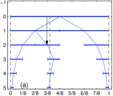
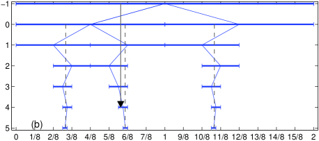
Figure 10: (a) Example of a dyadic decomposition of the unit interval with three boundary points $\{0,~{}0.4,~{}1\}$ (shown by vertical dashed lines) and the related tree of subintervals at five levels ($\varepsilon=2^{-5}$). For a test point $x=0.37$ (shown by arrow), one uses its binary expansion $x=0.01011\ldots$ to navigate over the tree. The descend is stopped at level $n=2$ since $x\notin I_{33}=[3/8,4/8]$. However, the rough estimate, $2^{-n-1}=0.125$, of the distance between $x$ and the boundary, $|x-\partial\Omega|=|0.37-0.4|=0.03$, obviously fails. To apply the $1/3$-trick, one constructs the dyadic decomposition for the boundary points shifted by $1/3$ (b). In this tree, the descent for the point $x+1/3$ is stopped at level $n^{\prime}=4$. The combined lower estimate $2^{-\max\{n,n^{\prime}\}}/6=2^{-4}/6\approx 0.0104$ is valid.

Once a dyadic decomposition for a given boundary is constructed, it can be used to estimate the distance to the boundary from any point $x$. In fact, one can easily (and very rapidly) find the smallest subinterval $I_{n,\lfloor 2^{n}x\rfloor}$ containing simultaneously $x$ and some boundary point. For this purpose, one starts from the “root” vertex and descends on the tree using the bits of $x$ to choose left or right edges at each scale. The descend is stopped when there is no edge to follow (Fig. 10a). Once the smallest common interval $I_{n,\lfloor 2^{n}x\rfloor}$ is found, there are two option: either $n=\lfloor\log_{2}(1/\varepsilon)\rfloor$ so that the point $x$ is indistinguishable from some boundary point at scale $\varepsilon$, and the distance estimate is set to $0$; or $n<\lfloor\log_{2}(1/\varepsilon)\rfloor$, and the distance to the boundary can be roughly estimated as $2^{-n-1}$ since the next subdivision must separate the point $x$ from the boundary points. However, this simplistic argument fails when the point $x$ and the closest boundary point lie on opposite sides of the midpoint of the smallest common interval $I_{n,\lfloor 2^{n}x\rfloor}$, but very close to each other. Although the next subdivision separates these two points, the distance between them can be arbitrarily small so that the rough estimate $2^{-n-1}$ is wrong, as illustrated on Fig. 10a. To get the correct lower estimate, one can apply the so-called “1/3-trick”.

IV.3 The 1/3-trick

The $1/3$-trick can be easily illustrated for two points $x$ and $y$. Let $I_{n,\lfloor 2^{n}x\rfloor}$ be the smallest common interval containing both points $x$ and $y$. Suppose that the distance between these points is smaller than $2^{-n}/6$. We consider the points $x^{\prime}=x+1/3$ and $y^{\prime}=y+1/3$ (shifted by $1/3$), and determine their smallest common interval $I_{n^{\prime},\lfloor 2^{n^{\prime}}x^{\prime}\rfloor}$. As shown in Appendix C, the distance between the points $x^{\prime}$ and $y^{\prime}$ (and thus between the points $x$ and $y$) is larger than $2^{-n^{\prime}}/6$. It is thus sufficient to find the smallest common intervals for the pair $x,y$ and its shifted counterpart $x^{\prime},y^{\prime}$, and the distance between the points is bounded below as

$$|x-y|=|x^{\prime}-y^{\prime}|\geq 2^{-\max\{n,n^{\prime}\}}/6.$$

This simple fact allows one to rapidly estimate the distance to boundary points. Let us consider a new boundary $\partial\Omega^{\prime}$ which is obtained by shifting the old one by $1/3$: $\partial\Omega^{\prime}=\{x\in{\mathbb{R}}~{}:~{}x-1/3\in\partial\Omega\}$. For the new boundary, another dyadic tree of subintervals can be constructed (Fig. 10b) in order to estimate the distance between $\partial\Omega^{\prime}$ and the shifted point $x^{\prime}=x+1/3$ at a given scale $\varepsilon$. While this construction may appear redundant at first thought because $|x-\partial\Omega|=|x^{\prime}-\partial\Omega^{\prime}|$, the crucial point is that we search for a lower estimate at a finite scale at which two dyadic trees are different. Performing the descend over both dyadic trees (using the binary expasion of $x$ and $x^{\prime}$, respectively), one identifies the level $n$ (resp. $n^{\prime}$) of the smallest common interval of $x$ (resp. $x^{\prime}$) and the closest boundary point (resp. shifted closest boundary point). The lower estimate of the distance is then

$$|x-\partial\Omega|=|x^{\prime}-\partial\Omega^{\prime}|\geq 2^{-\max\{n,n^{\prime}\}}/6.$$

IV.4 Higher dimensions

Similar constructions are applicable in higher dimensions which are more relevant for applications. The lower estimate relies on the generalized mean inequality:

$$M_{q}(c_{1},\ldots,c_{n})\leq M_{p}(c_{1},\ldots,c_{n})\qquad(q<p),$$ (43)

where the generalized mean $M_{p}(c_{1},\ldots,c_{n})$ of $n$ positive numbers $c_{1},\ldots,c_{n}$ is

$$M_{p}(c_{1},\ldots,c_{n})=\left(\frac{1}{n}\sum\limits_{k=1}^{n}c_{k}^{p}\right)^{1/p}.$$ (44)

Setting $q=1$, $p=2$, and $c_{k}=|x_{k}-y_{k}|$ for two points $x=(x_{1},\ldots,x_{d})$ and $y=(y_{1},\ldots,y_{d})$, Eq. (43) yields the lower estimate of their Euclidean distance:

$$|x-y|=\left(\sum\limits_{k=1}^{d}(x_{k}-y_{k})^{2}\right)^{1/2}\geq\frac{1}{\sqrt{d}}\sum\limits_{k=1}^{d}|x_{k}-y_{k}|.$$ (45)

Constructing two dyadic trees for each coordinate as earlier, one can then estimate each term $|x_{k}-y_{k}|$ and thus the distance from any point $x=(x_{1},\ldots,x_{d})$ to the boundary. In high dimensions ($d\gg 1$), the right-hand side of the inequality (45) is strongly attenuated by the prefactor $1/\sqrt{d}$. This is an example of the so-called “curse of dimensionality”. To overcome this difficulty, one can implement random rotations and translations of the boundary. Although these transformations preserve the distance, they can improve the lower bound at a finite scale. Note that other multiscale constructions and the related searchable data structures can also be used such as Whitney decompositions of the computational domain (in which the size of each square (or cube) paving the domain is comparable to the distance to the boundary), quadtrees (or Q-trees), k-d trees, etc. deBerg .

IV.5 Overall efficiency

The advantages of multiscale dyadic trees are numerous: the simplicity of construction, the generality of boundary shapes, the rapidity of distance estimation, the flexibility for shape modifications, and low memory usage. In fact, for a given precision $\varepsilon$, the storage of the dyadic tree requires at worst $N\log_{2}(1/\varepsilon)$ intervals (i.e., $\log_{2}(1/\varepsilon)$ levels for each boundary point, for $N$ points). In practice, this number is much smaller since many boundary points share the same interval at larger scales (e.g., the interval of size $1$ is shared by all boundary points).

The crucial point is that geometrical structure of the boundary does not matter at all: the method works for a random Cantor dust as well as for a circle. Moreover, the tree-like representation is highly adaptive, allowing one to modify the boundary from one set of simulations to other (or even from one run to the other). This feature can be very useful to study diffusion-controlled growth processes like DLA or transport phenomena in domains with moving boundaries.

V Conclusions

In this paper, we revised the multiscale construction of Gaussian processes and fields. First, the Haar wavelet representation of Brownian motion was explicitly constructed as a natural way to refine the geometrical features of a Brownian path under magnification. Since the Haar functions form a complete basis in the space $L^{2}([0,1])$ and their weights are Gaussian, such a representation can be extended to any complete basis $\{\psi_{i}(t)\}$ of $L^{2}([0,1])$, wavelet-like or not. In other words, the construction of Brownian motion has two separate “ingredients”: deterministic functions $\psi_{i}(t)$ capturing geometrical details, and their random weights $\hat{a}_{i}$. The choice of the functions $\psi_{i}(t)$ is voluntary that gives a certain freedom and flexibility in dealing with different problems. Qualitatively, this choice determines the way of connecting successive positions of Brownian motion at a given scale. On the opposite, the random weights determine the intrinsic stochastic properties of Brownian motion, independently of our choice of the basis $\{\psi_{i}(t)\}$.

The multiscale construction gives not only a simple closed formula for Brownian motion, but reveals its fundamental properties. For instance, continuity and non-differentiability of Brownian paths naturally follow from this construction. In addition, we discussed a closed mapping from the sampling unit interval onto the space of Brownian paths. Sampling Brownian paths can therefore be formally reduced to picking up a real number $\omega$ with the uniform measure. This construction does not require elaborate notions from modern probability theory such as Wiener measures, sigma-algebras, filtrations, etc. Although these notions are useful, the explicit multiscale construction is much easier for non-mathematicians.

These concepts are not limited to Brownian motion. We illustrated how fractional Brownian motion, Gaussian free field, and fractional Gaussian fields can be constructed in a very similar way. Extensions to other Gaussian processes were also mentioned. Finally, we briefly discussed how the multiscale concepts can be used for simulating restricted diffusion (i.e., Brownian motion in confining domains). The dyadic subdivision and the related hierarchical (multiscale) tree of subintervals allow one to rapidly estimate the distance to the boundary and thus to generate random displacements adapted to the local geometrical environment. Such fast random walk algorithms have found numerous applications. As for usual Brownian motion, dyadic decompositions appear as natural tools to store and rapidly access the geometrical information, resulting in fast algorithms.

Appendix A Conditional law

We explain why the distribution of the position of Brownian motion $y=B(1/2)$ at time $t=1/2$ under conditions $B(0)=0$ and $B(1)=x$ is given by the normal law ${\mathcal{N}}(x/2,1/4)$.

Since the increments of Brownian motion on the unit intervals $(0,1/2)$ and $(1/2,1)$ are independent, the joint probability density $p\{B(1/2)=y,~{}B(1)=x\}$ is simply equal to the product of the probability density $p\{B(1/2)-B(0)=y\}$ to have the first increment equal to $y$ and the probability density $p\{B(1)-B(1/2)=x-y\}$ to have the second increment equal to $x-y$. These densities are given by normal laws with variance $1/2$, yielding

$$\begin{split}p\{B(1/2)=y,~{}B(1)=x\}&=\left(\frac{e^{-\frac{y^{2}/2}{1/2}}}{\sqrt{2\pi}\sqrt{1/2}}\right)\left(\frac{e^{-\frac{(x-y)^{2}/2}{1/2}}}{\sqrt{2\pi}\sqrt{1/2}}\right)\\ &=\left(\frac{e^{-\frac{(y-x/2)^{2}/2}{1/4}}}{\sqrt{2\pi}\sqrt{1/4}}\right)\left(\frac{e^{-x^{2}/2}}{\sqrt{2\pi}}\right).\\ \end{split}$$

The second factor is simply the probability density for $x=B(1)$, while the first factor is the conditional probability density we are looking for:

$$p\{B(1/2)=y~{}|~{}B(1)=x\}=\frac{e^{-\frac{(y-x/2)^{2}/2}{1/4}}}{\sqrt{2\pi}~{}\sqrt{1/4}}.$$

This is the normal distribution with the mean $x/2$ and the variance $1/4$.

Appendix B Continuity and non-differentiability of Brownian motion

In this section, we illustrate how the wavelet representation of Brownian motion can be used to prove its basic properties such as continuity and non-differentiability.

B.1 Continuity and convergence

First, we show that a partial sum approximation converges to Brownian motion in both $L^{\infty}$ and $L^{2}$ norms. Let us denote

$$F_{n}(t)=\sum\limits_{k=0}^{2^{n}-1}a_{nk}h_{nk}(t)$$ (46)

so that $B(t)=a_{0}t+F_{0}(t)+F_{1}(t)+\ldots$ according to Eq. (7). Each function $F_{n}$ is a sum of hat functions with disjoint supports. To estimate the size of $F_{n}$ we need some upper bound on $a_{nk}$. We are going to show that $|a_{nk}|<n$ for all sufficiently large $n$.

Since $a_{nk}\in{\mathcal{N}}(0,1)$ are standard normal variables, we observe that

$${\mathbb{P}}(|a_{nk}|\geq n)=2\int\limits_{n}^{\infty}dz~{}\frac{e^{-z^{2}/2}}{\sqrt{2\pi}}\leq e^{-n^{2}/2}$$

for sufficiently large $n$. This inequality yields

$$\sum\limits_{n=0}^{\infty}\sum\limits_{k=0}^{2^{n}-1}{\mathbb{P}}(|a_{nk}|\geq n)\leq\sum\limits_{n=0}^{\infty}2^{n}e^{-n^{2}/2}<\infty.$$

By Borel-Cantelli lemma this implies that $|a_{nk}|<n$ for all but finitely many coefficients $a_{nk}$. In other words, almost surely, there is finite, but random, $N^{*}$ such that $|a_{nk}|<n$ if $n>N^{*}$. For such $n$ we have

$$\|F_{n}\|_{L^{\infty}([0,1])}=2^{-n/2-1}\max_{k}\{|a_{nk}|\}<n2^{-n/2-1}.$$

Since the sum of these norms converges, the series $a_{0}t+\sum_{n}F_{n}(t)$ converges to $B(t)$ in $L^{\infty}$ norm (uniformly), i.e. for any $\epsilon>0$

$$\lim\limits_{N\to\infty}{\mathbb{P}}\left\{\left\|B(t)-B_{N}(t)\right\|_{L^{\infty}([0,1])}>\epsilon\right\}=0,$$ (47)

where

$$B_{N}(t)=a_{0}t+\sum\limits_{n=0}^{N}\sum\limits_{k=0}^{2^{n}-1}a_{nk}h_{nk}(t)$$ (48)

is a partial sum approximation of Brownian motion at scale $2^{-N}$. This proves that Brownian motion is almost surely continuous. Moreover, the remainder of a partial sum approximation at scale $2^{-N}$ is exponentially small:

$$\left\|B(t)-B_{N}(t)\right\|_{L^{\infty}}<\sum\limits_{n=N+1}^{\infty}\left\|F_{n}(t)\right\|_{L^{\infty}}<\frac{3(N+3)}{2^{1+N/2}},$$ (49)

when $N$ is large enough.

The $L^{2}$ convergence can be shown in the same way. We have

$$\|F_{n}\|^{2}_{L^{2}([0,1])}=\sum\limits_{k=0}^{2^{n}-1}|a_{nk}|^{2}\|h_{nk}\|^{2}_{L^{2}([0,1])}<2^{n}~{}n^{2}~{}2^{-2n},$$

where we used $|a_{nk}|<n$ for large enough $n$. This inequality implies the convergence of $\sum_{n}\|F_{n}\|_{L^{2}([0,1])}$ with probability one and hence the series in Eq. (7) converges almost surely in $L^{2}$ norm:

$$\lim\limits_{N\to\infty}{\mathbb{E}}\left\{\left\|B(t)-B_{N}(t)\right\|_{L^{2}([0,1])}\right\}=0.$$ (50)

Both statements (47, 50) can be extended to arbitrary spectral representation of Brownian motion. Note also that these statements are applicable pointwise, e.g.,

$$\lim\limits_{N\to\infty}{\mathbb{E}}\left\{\left|B(t)-B_{N}(t)\right|\right\}=0$$ (51)

for any $t\in[0,1]$.

B.2 Nowhere differentiability

Since Brownian motion is a sum of hat functions it is easy to believe that $B(t)$ it not differentiable almost everywhere. One can prove a much stronger statement that $B(t)$ is nowhere differentiable with probability one. The proof goes along the same lines as for convergence (the argument follows the proof from Morters ).

We are going to show that almost surely for all $t$ at least one of the two limits,

$$\begin{split}\overline{B}^{\prime}(t)&=\limsup\frac{B(t+h)-B(t)}{h},\\ \underline{B}^{\prime}(t)&=\liminf\frac{B(t+h)-B(t)}{h}.\\ \end{split}$$

is infinite. This obviously implies that $B(t)$ is almost surely nowhere differentiable. Note that at local extrema, one of these limits can be finite, so it is not true that both of them are always infinite.

Let us assume that there is $t_{0}$ such that both limits are finite at $t_{0}$. This implies that there is a random finite constant $M$ such that

$$\left|\frac{B(t_{0}+h)-B(t_{0})}{h}\right|<M$$ (52)

for all $h$. For a given scale $n$, let $k$ be such that $t_{0}$ is between dyadic points $t_{n,k-1}$ and $t_{n,k}$, where $t_{n,k}\equiv 2^{-n}k$. The triangle inequality implies that for any $j$

$$\begin{split}&|B(t_{n,k+j})-B(t_{n,k+j-1})|<|B(t_{n,k+j})-B(t_{0})|\\ &+|B(t_{n,k+j-1})-B(t_{0})|<M(2j+1)2^{-n}.\\ \end{split}$$

Let $E_{nk}$ be the event that this inequality holds for $j=1,2,3$. Since increments are independent normal variables, one gets ${\mathbb{P}}\{E_{nk}\}\leq c(2^{-n/2})^{3}$, where $c$ is a constant. The probability that these inequalities hold for some $k$ from $0$ to $2^{n}-1$ is then bounded by $2^{n}(c2^{-3n/2})=c2^{-n/2}$. The sum of these probabilities over $n$ is finite, hence by Borel-Cantelli lemma, with probability one only finitely many of them will occur. On the other hand the assumed inequality (52) implies that infinitely many of $E_{nk}$ will occur. This yields the contradiction and proves that (52) cannot be true.

Appendix C The 1/3-trick to estimate the distance

Although the 1/3-trick is classical in analysis, we provide some explanations which may be instructive for non-experts.

The trick is based on a very simple result. Let $I_{nk}=[k2^{-n},(k+1)2^{-n})$ and its boundary $\partial I_{nk}=\{k2^{-n},(k+1)2^{-n}\}$. For any real $x$ and any integer $n$, there exist two intervals $I_{nk}$ and $I_{nk^{\prime}}$ of the same length $2^{-n}$ that $x$ belongs to $I_{nk}$ and $x^{\prime}=x+1/3$ belongs to $I_{nk^{\prime}}$. If the distance from $x$ to the boundary of $I_{nk}$ is smaller than $2^{-n}/6$, then the distance from $x^{\prime}$ to the boundary of $I_{nk^{\prime}}$ is larger than $2^{-n}/6$, and vice-versa. In other words, the point $x$ and the shifted point $x^{\prime}$ cannot be simultaneously close to the interval endpoints.

Suppose the opposite is true, so that

$$|2^{n}x-\hat{k}|<1/6,\qquad|2^{n}(x+1/3)-\hat{k}^{\prime}|<1/6,$$

where the integers $\hat{k}=k+[2(2^{n}x-k)]$ and $\hat{k}^{\prime}=k^{\prime}+[2(2^{n}x^{\prime}-k^{\prime})]$ denote the closest endpoint to $x$ and $x^{\prime}$, respectively. Since $2^{n}/3=k_{0}+(-1)^{n}/3$ with an integer $k_{0}$, the point $2^{n}x$ should be simultaneously within the distance $1/6$ to $\hat{k}$ and $\hat{k}^{\prime}+k_{0}+(-1)^{n}/3$ that is impossible since the distance between these points is larger than $1/3$ (Fig. 11):

$$\begin{split}\frac{1}{3}&\leq|(\hat{k}^{\prime}+k_{0}+(-1)^{n}/3)-\hat{k}|\leq|2^{n}x-\hat{k}|\\ &+|2^{n}x-(\hat{k}^{\prime}+k_{0}+(-1)^{n}/3)|<1/3.\\ \end{split}$$

Figure 11: Illustration for the proof of the $1/3$-trick. In this example, $\hat{k}=\hat{k^{\prime}}+k_{0}=k$ and $n$ is even.

Using this simple result, one can prove the estimate for the distance from a given point $x$ to the set of boundary points $\{y_{m}\}$. Let $I_{nk}$ be the largest interval containing $x$ and not containing any boundary point $y_{m}$. Similarly, for the shifted point $x^{\prime}=x+1/3$, let $I_{n^{\prime}k^{\prime}}$ be the largest interval containing $x^{\prime}$ and not containing any shifted boundary point $y_{m}^{\prime}=y_{m}+1/3$. Then the distance from $x$ to the set of boundary points $\{y_{m}\}$ is larger than $2^{-\max\{n,n^{\prime}\}}/6$.

Suppose that $n\geq n^{\prime}$. Assume that the statement is false so there exists a boundary point $y\in\{y_{m}\}$ such that $|x-y|<2^{-n}/6$. Suppose that $y<x$ (the opposite case is similar). Since $x\in I_{nk}$ and $y\notin I_{nk}$, both points $x$ and $y$ should be close to the endpoint $k2^{-n}$:

$$|x-k2^{-n}|<2^{-n}/6,\hskip 14.22636pt|y-k2^{-n}|<2^{-n}/6.$$

The shifted boundary point $y^{\prime}$ belongs to some interval $I_{nj}$. According to the previous result, the second inequality implies that the shifted point $y^{\prime}$ cannot be close to the endpoints of $I_{nj}$:

$$2^{-n}(j+1/6)\leq y^{\prime}\leq 2^{-n}(j+5/6).$$

Since $|x^{\prime}-y^{\prime}|=|x-y|<2^{-n}/6$ and $y<x$, then $y^{\prime}<x^{\prime}<y^{\prime}+2^{-n}/6$, hence

$$2^{-n}(j+1/6)\leq x^{\prime}<2^{-n}(j+1),$$

i.e., the point $x^{\prime}$ belongs to the same interval $I_{nj}$ as $y^{\prime}$. At the same time, $x^{\prime}$ belongs to $I_{n^{\prime}k^{\prime}}$ which is larger than $I_{nj}$ due to $n\geq n^{\prime}$. The dyadic structure implies that $I_{nj}\subset I_{n^{\prime}k^{\prime}}$ so that $y^{\prime}$ should belong to $I_{n^{\prime}k^{\prime}}$ as well. But this is in contradiction with the initial assumption about $I_{n^{\prime}k^{\prime}}$.

References

- (1) D. R. J. Revuz and M. Yor, Continuous Martingales and Brownian Motion (Berlin: Springer, 1999).
- (2) K. Itô and H. P. McKean, Diffusion Processes and Their Sample Paths (Berlin: Springer-Verlag, 1965).
- (3) S. C. Port and C. J. Stone, Brownian Motion and Classical Potential Theory (New York: Academic Press, 1978).
- (4) R. F. Bass, Diffusions and Elliptic Operators (Springer, 1998).
- (5) A. N. Borodin and P. Salminen, Handbook of Brownian Motion: Facts and Formulae (Basel-Boston-Berlin: Birkhauser Verlag, 1996).
- (6) P. Lévy, Processus Stochastiques et Mouvement Brownien (Paris, Gauthier-Villard, 1965).
- (7) B. B. Mandelbrot, The Fractal Geometry of Nature (Freeman, San Francisco, New York, 1982).
- (8) E. R. Weibel, The Pathway for oxygen. Structure and function in the mammalian respiratory system (Harvard University, Cambridge, Massachusetts and London, England, 1984).
- (9) S. Jaffard, Y. Meyer, and R. D. Ryan, Wavelets: Tools for Science and Technology, (SIAM, Philadelphia, 2001).
- (10) I. Daubechies, Ten Lectures on Wavelets, CBMS-NSF Regional Conf. Series in Applied Mathematics, vol. 61, Society for Industrial and Applied Mathematics (SIAM) (Philadelphia, PA, 1992).
- (11) S. Mallat, A Wavelet Tour of Signal Processing: The Sparse Way, 3rd Ed. (Academic Press, 2008).
- (12) A. R. Mehrabi and M. Sahimi, “Coarsening of Heterogeneous Media: Application of Wavelets”, Phys. Rev. Lett. 79, 4385-4388 (1997).
- (13) F. Ebrahimi and M. Sahimi, Multiresolution Wavelet Scale Up of Unstable Miscible Displacements in Flow Through Heterogeneous Porous Media, Trans. Porous Media 57, 75-102 (2004).
- (14) R. Friedrich, J. Peinke, M. Sahimi, and M. R. R. Tabar, Approaching complexity by stochastic methods: From biological systems to turbulence, Phys. Rep. 506, 87-162 (2011).
- (15) J. M. Bardeen, J. R. Bond, N. Kaiser, and A. S. Szalay, “The statistics of peaks of Gaussian random fields”, Astrophys. J. 304, 15-61 (1986).
- (16) N. Kobayashi, Y. Yamazaki, H. Kuninaka, M. Katori, M. Matsushita, S. Matsushita, and L.-Y. Chiang, “Fractal Structure of Isothermal Lines and Loops on the Cosmic Microwave Background”, J. Phys. Soc. Japan 80, 074003 (2010).
- (17) R. Fernandez, J. Fröhlich, and A. D. Sokal, Random Walks, Critical Phenomena, and Triviality in Quantum Field Theory (Texts and Monographs in Physics. Springer, Berlin Heidelberg, New York, 1992).
- (18) S. Dodelson, Modern Cosmology (Academic Press, Amsterdam, Netherlands, 2003).
- (19) R. Brown, “A brief account of microscopical observations made in the months of June, July and August, 1827, on the particles contained in the pollen of plants; and on the general existence of active molecules in organic and inorganic bodies”, Edinburgh New Phil. J. 5, 358-371 (1828).
- (20) J. Perrin, “L’agitation moleculaire et le mouvement brownien”, Compt. Rendus Herbo. Seances Acad. Sci. Paris 146, 967 (1908).
- (21) J. Perrin, “Mouvement brownien et realite moleculaire”, Ann. Chim. Phys. 18, 1-114 (1909).
- (22) W. Feller, An Introduction to Probability Theory and Its Applications, Volumes I and II, Second Edition (John Wiley & Sons, New York, 1971).
- (23) J.-P. Bouchaud and A. Georges, “Anomalous diffusion in disordered media: Statistical mechanisms, models and physical applications”, Phys. Rep. 195, 127-293 (1990).
- (24) R. Metzler and J. Klafter, “The random walk’s guide to anomalous diffusion: a fractional dynamics approach”, Phys. Rep. 339, 1-77 (2000).
- (25) M. F. Shlesinger, J. Klafter, and G. Zumofen, “Above, below and beyond Brownian motion”, Am. J. Phys. 67, 1253-1259 (1999).
- (26) M. Loève, Probability theory, Vol. II, 4th ed., Graduate Texts in Mathematics, Vol. 46 (Springer-Verlag, 1978).
- (27) B. Alpert, Sparse representation of smooth linear operators, Ph.D. thesis, Department of Computer Science (Yale University, 1990).
- (28) B. Alpert, “Construction of Simple Multi-scale Bases for Fast Matrix Operations”, in Wavelets and Their Applications, ed. by Ruskai, Beylkin, Coifman, Daubechies, Mallat, Mayer, and Raphael (Jones & Bartlett, Boston, 1992), p. 211.
- (29) G. Beylkin, R. Coifman, V. Rokhlin, “Fast wavelet transforms and numerical algorithms I”, Comm. Pure Appl. Math. 44 141-183 (1991).
- (30) G. Beylkin, R. Coifman, and V. Rokhlin, “Wavelets in Numerical Analysis”, in Wavelets and Their Applications, ed. by Ruskai, Beylkin, Coifman, Daubechies, Mallat, Mayer, and Raphael (Jones & Bartlett, Boston, 1992), p. 181.
- (31) F. W. Elliott and A. J. Majda, “A Wavelet Monte Carlo Method for Turbulent Diffusion with Many Spatial Scales”, J. Comput. Phys. 113, 82-109 (1994).
- (32) A. N. Kolmogorov, “Wienersche Spiralen und einige andere interessante Kurven im Hilbertschen Raum.” C. R. (Doklady) Acad. Sci. URSS (N. S.) 26, 115-118 (1940).
- (33) B. B. Mandelbrot and J. W. Van Ness, “Fractional Brownian motions, fractional noises and applications”, SIAM Rev. 10 422-437 (1968).
- (34) M. Lesieur, Turbulence in Fluids (Kluwer Academic, Boston, 1990).
- (35) W. McComb, The Physics of Fluid Turbulence (Clarendon Press, Oxford, 1990).
- (36) A. J. Majda and P. R. Kramer, “Simplified models for turbulent diffusion: Theory, numerical modelling, and physical phenomena”, Phys. Rep. 314, 237-574 (1999).
- (37) F. W. Elliott and A. J. Majda, “A New Algorithm with Plane Waves and Wavelets for Random Velocity Fields with Many Spatial Scales”, J. Comput. Phys. 117, 146-162 (1995).
- (38) F. W. Elliott, A. J. Majda, D. J. Horntrop, and R. M. McLaughlin, “Hierarchical Monte Carlo Methods for Fractal Random Fields”, J. Stat. Phys. 81, 717-735 (1995).
- (39) F. W. Elliott, D. J. Horntrop, and A. J. Majda, “A Fourier-Wavelet Monte Carlo Method for Fractal Random Fields”, J. Comput. Phys. 132, 384-408 (1997).
- (40) The Science of Disasters: Climate Disruptions, Heart Attacks, and Market Crashes, Eds. A. Bunde, J. Kropp, and H. J. Schellnhuber (Springer-Verlag, Berlin, Heidelberg, 2002).
- (41) B. Mandelbrot, Fractals and scaling in finance: discontinuity, concentration, risk (New York, Springer, 1997).
- (42) P. Lévy, “Random functions: General theory with special references to Laplacian random functions”, Univ. California Publ. in Statist. 1, 331-390 (1953).
- (43) L. Decreusefond and A. Üstünel, “Stochastic analysis of the fractional Brownian motion”, Poten. Anal. 10, 177-214 (1999).
- (44) G. W. Wornell, “A Karhunen-Loéve like expansion for 1/f processes via wavelets, IEEE Trans. Inform. Theory 36, 859-861 (1990).
- (45) P. Flandrin, “Wavelet analysis and synthesis of fractional Brownian motion”, IEEE Trans. Inform. Theory 38, 910-917 (1992).
- (46) F. Sellan, “Synthèse de mouvements browniens fractionnaires à l’aide de la transformation par ondelettes”, Compte Rendus Acad. Sci. Paris Série I 321, 351-358 (1995).
- (47) P. Abry and F. Sellan, “The wavelet-based synthesis for fractional brownian motion proposed by F. Sellan and Y. Meyer: Remarks and fast implementation”, Appl. Comput. Harm. Anal. 3, 377-383 (1996).
- (48) R. B. Davies and D.S. Harte, “Tests for Hurst effect”, Biometrika 74, 95-102 (1987).
- (49) A. T. A. Wood and G. Chan, “Simulation of stationary Gaussian processes in ”, J. Comput. Graph. Stat. 3, 409-432 (1994).
- (50) C. R. Dietrich and G. N. Newsam, “Fast and exact simulation of stationary Gaussian processes through circulant embedding of the covariance matrix”, SIAM Journal Sci. Comput. 18, 1088-1107 (1997).
- (51) A. Fournier, D. Fussel, and L. Carpenter, “Computer Rendering of Stochastic Models”, Commun. ACM 25, 371-384 (1982).
- (52) G. E. Uhlenbeck and L. S. Ornstein, “On the theory of the Brownian motion”, Phys. Rev. 36, 823 (1930).
- (53) H. Risken, The Fokker-Planck equation: methods of solution and applications, 3rd Ed. (Berlin: Springer, 1996).
- (54) W. T. Coffey, Y. P. Kalmykov, and J. T. Waldron, The Langevin equation: with applications to stochastic problems in physics, chemistry and electrical engineering, 2nd Ed. (World Scientific Publishing, Singapore, 2004).
- (55) S. Sheffield, “Gaussian free fields for mathematicians”, Probab. Theory Relat. Fields 139, 521-541 (2007).
- (56) A. Lodhia, S. Sheffield, X. Sun, and S. S. Watson, “Fractional Gaussian fields: a survey”, ArXiv 1407.5598 [math.PR].
- (57) B. Duplantier, R. Rhodes, S. Sheffield, and V. Vargas, “Log-correlated Gaussian fields: an overview” ArXiv 1407.5605v1 [math.PR].
- (58) R. J. Adler, Geometry of random fields, (Wiley & Sons, 1981).
- (59) R. J. Adler and J. E. Taylor, Random Fields and Geometry (Springer Monographs in Mathematics, 2007).
- (60) E. Vanmarcke, Random Fields: Analysis and Synthesis (World Scientific Publishing Company, 2010).
- (61) M. V. Berry, “Regular and irregular semiclassical wavefunctions”, J. Phys. A: Math. Gen. 10, 2083 (1977).
- (62) F. Nazarov and M. Sodin, “Random complex zeroes and random nodal lines”, Proc. Int. Congress Math, Volume III, 1450-1484 (Hindustan Book Agency, New Delhi, 2010).
- (63) J. Kondev and C. L. Henley, “Geometrical Exponents of Contour Loops on Random Gaussian Surfaces”, Phys. Rev. Lett. 74, 4580 (1995).
- (64) O. Schramm and S. Sheffield, “Contour lines of the two-dimensional discrete Gaussian free field”, Acta Math. 202, 21-137 (2009).
- (65) Z.-Q. Chen, P. Kim, and R. Song, “Heat kernel estimates for the Dirichlet fractional Laplacian”, J. Eur. Math. Soc. 12, 1307-1329 (2010).
- (66) R. Courant and D. Hilbert, Methods of Mathematical Physics, Vol. I (Jonh Wiley & Sons, New York, 1937-1989).
- (67) D. S. Grebenkov and B.-T. Nguyen, “Geometrical structure of Laplacian eigenfunctions”, SIAM Rev. 55, 601-667 (2013).
- (68) P. T. Callaghan, Principles of Nuclear Magnetic Resonance Microscopy (Clarendon, Oxford, 1991).
- (69) D. S. Grebenkov, “NMR survey of reflected Brownian motion”, Rev. Mod. Phys. 79, 1077-1137 (2007).
- (70) B. Alberts, D. Bray, J. Lewis, M. Raff, K. Roberts, and J. D. Watson, Molecular Biology of the Cell, 3rd Ed. (Garland, New York, 1994).
- (71) P. C. Bressloff and J. M. Newby “Stochastic models of intracellular transport”, Rev. Mod. Phys. 85, 135-196 (2013).
- (72) O. Bénichou and R. Voituriez, “From first-passage times of random walks in confinement to geometry-controlled kinetics”, Phys. Rep. 539, 225-284 (2014).
- (73) G. Wilemski and M. Fixman, “General theory of diffusion-controlled reactions”, J. Chem. Phys. 58, 4009-4019 (1973).
- (74) M.-O. Coppens, “The Effect of Fractal Surface Roughness on Diffusion and Reaction in Porous Catalysts: from Fundamentals to Practical Applications”, Catalysis Today 53, 225-243 (1999).
- (75) B. Sapoval, “General Formulation of Laplacian Transfer Across Irregular Surfaces”, Phys. Rev. Lett. 73, 3314-3316 (1994).
- (76) B. Sapoval, “Transport Across Irregular Interfaces: Fractal Electrodes, Membranes and Catalysts”, in “Fractals and Disordered Systems”, Eds. A. Bunde, S. Havlin (Springer, Berlin, 1996).
- (77) D. S. Grebenkov, “Partially Reflected Brownian Motion: A Stochastic Approach to Transport Phenomena”, in “Focus on Probability Theory”, Ed. L. R. Velle, pp. 135-169 (Nova Science Publishers, 2006).
- (78) D. S. Grebenkov, “Scaling Properties of the Spread Harmonic Measures”, Fractals 14, 231-243 (2006).
- (79) A. Singer, Z. Schuss, A. Osipov, and D. Holcman, “Partially Reflected Diffusion”, SIAM J. Appl. Math. 68, 844-868 (2008).
- (80) S. Redner, A Guide to First-Passage Processes (Cambridge University Press, Cambridge, England, 2001).
- (81) K. K. Sabelfeld, Monte Carlo Methods in Boundary Value Problems (Springer-Verlag: New York - Heidelberg, Berlin, 1991).
- (82) K. K. Sabelfeld and N. A. Simonov, Random Walks on Boundary for Solving PDEs (Utrecht, The Netherlands, 1994).
- (83) G. N. Milstein, Numerical Integration of Stochastic Differential Equations (Kluwer, Dordrecht, the Netherlands, 1995).
- (84) D. S. Grebenkov, “Efficient Monte Carlo methods for simulating diffusion-reaction processes in complex systems”, in “First-Passage Phenomena and Their Applications”, Eds. R. Metzler, G. Oshanin, S. Redner (World Scientific Press, 2014).
- (85) M. E. Muller, “Some Continuous Monte Carlo Methods for the Dirichlet Problem”, Annals Math. Statist. 27, 569-589 (1956).
- (86) P. Meakin, “The structure of two-dimensional Witten-Sander aggregates”, J. Phys. A 18, L661 (1985).
- (87) P. Ossadnik, “Multiscaling Analysis of Large-Scale Off-Lattice DLA”, Physica A 176, 454 (1991).
- (88) D. S. Grebenkov, “What Makes a Boundary Less Accessible”, Phys. Rev. Lett. 95, 200602 (2005).
- (89) D. S. Grebenkov, A. A. Lebedev, M. Filoche, and B. Sapoval, “Multifractal Properties of the Harmonic Measure on Koch Boundaries in Two and Three Dimensions”, Phys. Rev. E 71, 056121 (2005).
- (90) S. Torquato and I. C. Kim, “Efficient simulation technique to compute effective properties of heterogeneous media”, Appl. Phys. Lett. 55, 1847 (1989).
- (91) L. H. Zheng and Y. C. Chiew, “Computer simulation of diffusion-controlled reactions in dispersions of spherical sinks”, J. Chem. Phys. 90, 322-327 (1989).
- (92) M. Leibig, “Random walks and NMR measurements in porous media”, J. Phys. A: Math. Gen. 26, 3349 (1993).
- (93) D. S. Grebenkov, “A fast random walk algorithm for computing the pulsed-gradient spin-echo signal in multiscale porous media”, J. Magn. Reson. 208, 243-255 (2011).
- (94) M. de Berg, M. van Kreveld, M. Overmars, and O. Schwarzkopf, Computational Geometry: Algorithms and Applications, 2nd ed. (Springer-Verlag, Berlin, 2000).
- (95) P. Mörters and Y. Peres, Brownian Motion (Cambridge Series in Statistical and Probabilistic Mathematics, Cambridge University Press, New York, 2010).