Localization, delocalization, and topological phase transitions in the one-dimensional split-step quantum walk

Abstract

Quantum walks are promising for information processing tasks because on regular graphs they spread quadratically faster than random walks. Static disorder, however, can turn the tables: unlike random walks, quantum walks can suffer Anderson localization, with their wavefunction staying within a finite region even in the infinite time limit, with a probability exponentially close to one. It is thus important to understand when a quantum walk will be Anderson localized and when we can expect it to spread to infinity even in the presence of disorder. In this work we analyze the response of a one-dimensional quantum walk – the split-step walk – to different forms of static disorder. We find that introducing static, symmetry-preserving disorder in the parameters of the walk leads to Anderson localization. In the completely disordered limit, however, a delocalization transition occurs, and the walk spreads subdiffusively to infinity. Using an efficient numerical algorithm, we calculate the bulk topological invariants of the disordered walk, and find that the disorder-induced Anderson localization and delocalization transitions are governed by the topological phases of the quantum walk.

I Introduction

Discrete-time Quantum WalksKempe (2003) (or, simply, quantum walks) are quantum mechanical generalizations of the random walk. Their hallmark property is that on a regular lattice they spread quadratically faster than random walks, i.e., ballistically rather than diffusively. This makes them valuable in quantum search algorithmsShenvi et al. (2003), or even for general quantum computing Lovett et al. (2010). Experiments on quantum walks range from realizations on trapped ionsTravaglione and Milburn (2002); Zähringer et al. (2010); Schmitz et al. (2009), cold atoms in optical latticesKarski et al. (2009); Genske et al. (2013); Robens et al. (2015), to light on an optical tableSchreiber et al. (2010, 2012); Peruzzo et al. (2010); Broome et al. (2010); Sansoni et al. (2012); Zhao et al. (2015), but there are many other experimental proposalsCôté et al. (2006); Kálmán et al. (2009).

The dynamics of a quantum walk is given by iterations of a unitary timestep operator, which can always be written in the form $U=e^{-iH_{\textrm{eff}}}$, with $H_{\textrm{eff}}$ a hermitian operator. In this sense, a quantum walk is a stroboscopic simulator of an effective Hamiltonian $H_{\textrm{eff}}$. This is a powerful theoretical concept that allows much of the physical intuition about lattice systems to be applied to quantum walks. As an example, consider quantum walks on regular lattices: the maximum of the group velocity of the effective Hamiltonian translates directly to the velocity of ballistic expansion of the walk.

In the presence of static (time-independent) disorder, quantum walks can lose their advantage over random walks in terms of the speed of spreading: they can undergo Anderson localization, whereby the mean-squared distance of the walker from the origin stays bounded even in the infinite-time limit. Besides theoreticalJoye and Merkli (2010); Ahlbrecht et al. (2011) and numerical studiesDe Nicola et al. (2014), this effect has also been observed experimentallySchreiber et al. (2011).

There are special cases where quantum walks can evade Anderson localization and spread indefinitely even in the presence of static disorder. Already the simplest one-dimensional quantum walk with angle disorder presents such a case: rather than being completely localized, it spreads subdiffusivelyObuse and Kawakami (2011). This feature was explained in Ref. Obuse and Kawakami, 2011 by mapping the effective Hamiltonian of the quantum walk to chiral symmetric quantum wires (also see Ref. Zhao and Gong, 2015). With an eye towards potential applications of quantum walks, it is important to understand under what conditions we should expect Anderson localization, and when delocalized behaviour, of disordered quantum walks.

One of the key concepts that can help us understand when to expect Anderson localization in a quantum walkEdge and Asboth (2015), is that of topological phases. As noted in Ref. Kitagawa et al., 2010, the effective Hamiltonian $H_{\textrm{eff}}$ of a quantum walk on a regular lattice can be engineered to be that of a topological band insulatorHasan and Kane (2010). If that happens, bulk–boundary correspondenceHasan and Kane (2010) predicts that the quantum walk will host topologically protected edge states, whose number is given by a topological invariant of the bulk. These states can have a drastic influence on the time evolution of the walker if they have a large overlap with the initial state.

Quantum walks have been shown to have a broader range of topological phases than that of their effective HamiltonianAsbóth (2012): their topological invariants depend on details of how the timestep is performed. These invariants can be expressed as winding numbers of the bulk timestep operator over a part of the timestepAsbóth and Obuse (2013); Asbóth et al. (2014); Obuse et al. (2015), or using a generalization of the scattering theory of topological phases Fulga et al. (2012); Tarasinski et al. (2014). In this respect quantum walks are representative of the extreme limit of periodically driven systemsAsboth and Edge (2015); Jiang et al. (2011); Rudner et al. (2013); Cayssol et al. (2013), as is the (closely related) quantum kicked rotatorDahlhaus et al. (2011). In the case of the one-dimensional split-step quantum walk, topologically protected edge states not predicted by the invariants of the effective Hamiltonian have even been observed experimentallyKitagawa et al. (2012); the corresponding topological invariants have only recently been identifiedObuse et al. (2015).

In this paper we explore the relation between Anderson localization and topological phases for one-dimensional split-step quantum walks. This is a broad family of quantum walks with chiral and particle-hole symmetries, which contains as a special case the simple quantum walk of Ref. Obuse and Kawakami, 2011. We use a cloning procedure to derive the real-space scattering matrix of the walk, which allows us to give simple and efficient formulas for the topological invariants as well as for the localization lengths. We find that uniform disorder in the rotation angles, which does not break the symmetries, leads to Anderson localization in the generic case. At maximal angle disorder, however, there is a disorder-induced delocalization transition and the walk spreads (sub-)diffusively. We also obtain a simple interpretation of the delocalized behaviour of the simple quantum walk, by mapping it to a split-step walk at a boundary between topological phases. Finally, we explore the effects of symmetry breaking disorder using phase disorder, i.e., position-dependent but time-independent phase factor applied to the wave function after every timestep. We find that when this disorder breaks the symmetries of the system it invariably leads to Anderson localization.

This paper is structured as follows. In Sec. II we remind the reader of the definition of the split-step quantum walkKitagawa et al. (2010), of timeframes, and of the symmetries of this quantum walk. In Sec. III we derive our main result: the Lyapunov exponents of the split-step quantum walks, obtained through the real-space scattering matrix using a cloning procedure. In Sec. IV we apply this tool to treat uniform disorder in the rotation angles, find Anderson localization or delocalization depending on the parameters, and give a new perspective on the delocalization of the simple quantum walkObuse and Kawakami (2011). In Sec. V we discuss two types of phase disorder: one which breaks both symmetries of the quantum walk and thus leads to Anderson localization, and one which breaks only particle-hole symmetry, and leads to the same type of behaviour as disorder in the rotation angles. In Sec. VI we draw some conclusions. We also include pedagogically important examples and calculations in Appendices. In App. A we discuss the pedagogical case of split-step quantum walks with binary disorder. In App. B we calculate the critical exponent of the localization-delocalization transition. In App. C we calculate the topological invariants of the split-step walk using the noncommutative generalization of the winding numberMondragon-Shem et al. (2014).

II The Split-step quantum walk

In this work we consider the split-step quantum walk on a one-dimensional chain. The state of the walker at each integer time $t\in\mathbb{N}$ is represented by a wavefunction,

$$|{\Psi(t)}\rangle =\sum_{x=-\infty}^{\infty}\sum_{s=\uparrow,\downarrow}\psi(x,s,t)|{x,s}\rangle.$$ (1)

Here $x\in\mathbb{Z}$ is the coordinate and $s\in\{\uparrow,\downarrow\}$ is the internal degree of freedom, which we refer to as spin (in the quantum walk literature, the term “coin” is often used).

The quantum walk consists of a sequence of three types of operations. Spin-dependent shift operations displace the walker, but do not mix the two spin components,

$$S_{\uparrow} =\sum_{x}\big{(}|{x+1,\uparrow}\rangle\langle{x,\uparrow}|+|{x,\downarrow}\rangle\langle{x,\downarrow}|\big{)};$$ (2)

$$S_{\downarrow} =\sum_{x}\big{(}|{x,\uparrow}\rangle\langle{x,\uparrow}|+|{x-1,\downarrow}\rangle\langle{x,\downarrow}|\big{)}.$$ (3)

Spin rotation operators rotate the spin about the $y$ axis through a position-dependent angle,

$$R(\theta) =\sum_{x}\sum_{s=\uparrow,\downarrow}e^{-i\theta(x)\sigma_{y}}|{x,s}\rangle\langle{x,s}|.$$ (4)

Finally, phase operators multiply the wavefunction by a position- and spin-dependent phase factor,

$$P(\phi) =\sum_{x}\sum_{s=\uparrow,\downarrow}e^{-i\phi(x,s)}|{x,s}\rangle\langle{x,s}|.$$ (5)

The quantum walk is defined by a short sequence of operations which is then periodically repeated. The effect of this sequence is represented by the unitary timestep operator, which for the split-step walk reads

$$U(\theta_{1},\theta_{2}) =S_{\downarrow}R(\theta_{2})S_{\uparrow}R(\theta_{1}).$$ (6)

The time evolution is given by

$$|{\Psi(t+1)}\rangle =U(\theta_{1},\theta_{2})|{\Psi(t)}\rangle,$$ (7)

as represented in Fig. 1.

The simple quantum walk, as, e.g., in Ref. Obuse and Kawakami, 2011, has a single rotation operation per period. Its timestep reads

$$U_{s}(\theta) =S_{\downarrow}S_{\uparrow}R(\theta).$$ (8)

This can be seen as a special case of the split-step quantum walk, with $\theta_{2}=0$.

We will also consider the phase disordered quantum walk. The timestep operator of this walk reads

$$U_{p}(\phi,\theta_{1},\theta_{2}) =P(\phi)S_{\downarrow}R(\theta_{2})S_{\uparrow}R(\theta_{1}).$$ (9)

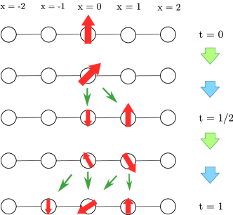
Figure 1: (Color online) A full timestep of the split-step walk, consisting of 4 operations: (1) rotation of the spin about the $y$ axis through angle $2\theta_{1}$, (2) displacement of the $s=+1$ component of the wavefunction to the right, (3) second spin rotation through angle $2\theta_{2}$, (4) displacement of the $s=-1$ component of the wavefunction to the left.

II.1 Timeframes, timestep operators, effective Hamiltonians

There is a considerable freedom in specifying a quantum walk, i.e., a periodic sequence of operations, corresponding to shifting the starting time of the period, which we refer to as changing the timeframe Asbóth and Obuse (2013). As an example, consider the operators

$$U(\theta_{1},\theta_{2})^{\prime} =R(\theta_{1}/2)S_{\downarrow}R(\theta_{2})S_{\uparrow}R(\theta_{1}/2);$$ (10)

$$U(\theta_{1},\theta_{2})^{\prime\prime} =R(\theta_{2}/2)S_{\uparrow}R(\theta_{1})S_{\downarrow}R(\theta_{2}/2).$$ (11)

These both correspond to the split-step quantum walk as defined by Eq. (11), only in different timeframes. Timestep operators describing the same quantum walk in different timeframes are related to each other by a unitary transformation.

The effective Hamiltonian $H_{\textrm{eff}}$ of a quantum walk is defined as the logarithm of the unitary timestep operator,

$$H_{\textrm{eff}} =i\text{ln}\,U.$$ (12)

The branch cut in the logarithm is taken along the negative real axis, and so all eigenvalues of $H_{\textrm{eff}}$, the quasienergies $E$, are between $-\pi$ and $\pi$. Since the unitary timestep operator $U$ depends on the choice of timeframe (initial time of the period), the same quantum walk has many, unitary equivalent effective Hamiltonians associated with it.

II.2 Symmetries and topological phases

The split-step walk has both particle-hole symmetry represented by complex conjugation $K$, and chiral symmetry, which places the system in Cartan class BDI Asbóth and Obuse (2013).

To see particle-hole symmetry of the quantum walk, notice that all matrix elements of the timestep operator $U(\theta_{1},\theta_{2})$ are real (in position and $\sigma_{z}$ basis). Thus,

$$KU(\theta_{1},\theta_{2})K =U(\theta_{1},\theta_{2}),$$ (13)

and therefore $KH_{\textrm{eff}}K=-H_{\textrm{eff}}$, which is the defining relation of particle-hole symmetry. This holds for the split-step quantum walk in the two timeframes defined by Eqs. (10) and (11) as well. We remark that for a periodically driven particle-hole symmetric Hamiltonian, the symmetry is inherited by the effective Hamiltonian in all timeframesJiang et al. (2011).

To see chiral symmetry of a quantum walk explicitly, it is necessary to go to a chiral symmetric timeframeAsbóth and Obuse (2013). In the case of the split-step walk, there are two such timeframes, specified by Eqs. (10) and (11). In these timeframes, we have

$$\sigma_{x}U(\theta_{1},\theta_{2})^{\prime}\sigma_{x} ={U(\theta_{1},\theta_{2})^{\prime}}^{\dagger},$$ (14)

and, consequently, $\sigma_{x}H_{\textrm{eff}}^{\prime}\sigma_{x}=-H_{\textrm{eff}}^{\prime}$, which is the defining relation of chiral symmetry. However, unlike particle-hole symmetry, the chiral symmetry requirement is nonlocal in timeAsbóth and Obuse (2013). The addition of a phase shift operation to the timestep, as in Eq. (9) breaks both time-reversal and chiral symmetries.

The presence of chiral symmetry enables us to assign bulk topological invariants to the quantum walk, similar to those in static systems. Due to the periodicity of the quasienergy, however, edge states – eigenstates of the chiral symmetry operator – can exist at either $E=0$ or $E=\pi$ quasienergies. This means that there are two different topological invariants, $\nu_{0}$ and $\nu_{\pi}$, associated with the bulk.

In the translation invariant case, when the angles $\theta_{1}$ and $\theta_{2}$ are the same for all coordinates, we can obtain the the topological invariants by calculating the winding number in both chiral timeframes given by (10) and (11). These two winding numbers can be combined to give the topological invariants $\nu_{0}$ and $\nu_{\pi}$ Asbóth and Obuse (2013), resulting in the topological phase map shown in Fig. 2

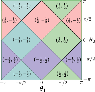
Figure 2: (Color online) Phase map of the split-step walk, with gapped phases indexed by their pair of bulk topological invariants, $(\nu_{0},\nu_{\pi})$. Along the continuous (dashed) lines, the quasienergy gap at $E=0$ ($E=\pi$) closes.

III Lyapunov exponents and topological invariants by cloning

In this paper we will be concerned with the effect of disorder on the topological invariants and edge states of the split-step walk. Since disorder breaks translation invariance, the bulk topological invariants can no longer be obtained as $k$-space winding numbers. There are two alternative approaches to the topological invariants for the disordered case: the one based on the scattering matrix Fulga et al. (2012); Tarasinski et al. (2014), and the one based on a reformulation of the winding number in real space, recently used for the disordered SSH modelMondragon-Shem et al. (2014). In the following we detail the first approach. In App. C we briefly describe the second approach, and compare the results obtained via these approaches.

To define a scattering matrix, we have to use open boundary conditions, with two translationally invariant leads attached to the scattering regionTarasinski et al. (2014). To obtain leads that host the right number of propagating modes, we omit the rotations in semi-infinite parts of the system, so the timestep operator there simply reads $U=S_{\downarrow}S_{\uparrow}$, as shown in Fig. 3.

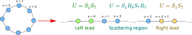
Figure 3: (Color online) To implement the scattering matrix for the quantum walk, we break up the periodic boundary conditions and attach two leads to the two ends of the system. The eigenstates in the leads are plane waves with linear dispersion relations.

The scattering theory of topological invariants gives a simple way to write down the topological invariants of a bulk: they are related to the reflection amplitudes of the bulk at the quasienergies of the edge states. Chiral symmetry ensures that the reflection amplitudes at these energies are real and the topological invariants for a bulk are given byTarasinski et al. (2014)

$$\nu_{E}=\frac{1}{2}r(E).\qquad(E=0,\pi)$$ (15)

The scattering matrix of a quantum chain of $L$ “slices” is usually obtained from the transfer matrix, which is the product of the $L$ transfer matrices representing the effect of each slice. The product structure of the transfer matrix makes it straightforward to obtain the statistical properties of a system with uncorrelated disorder, if the transfer matrix of each slice is obtained from variables that are local to the site.

There is a problem with applying the transfer matrix method directly to a split-step walk. During one timestep the walker makes excursions to nearest-neighbor sites and thus is not only affected by variables that are local to one site.

Our approach to dealing with this problem involves an extension of the Hilbert space, by introducing $N$ copies, or “clones” of the original split-step walk consisting of $N$ substeps. We explain the details below for the $N=2$ case, the generalization is straightforward.

III.1 Cloning

The central idea of cloning, as shown in Fig. 4, is that we double the number of internal degrees of freedom at each site, thus creating two clones, and we break up the time evolution between these clones. The first half of the step takes place on the first clone and the second part on the second clone. At the beginning of each step, the walker is shifted from one clone to the other by an operator $D$. In formulas,

$$U_{\text{cloned}}=SRD$$ (16a)

$$S =S_{\uparrow}\bigoplus S_{\downarrow}$$ (16b)

$$R =R_{1}\bigoplus R_{2}$$ (16c)

$$D =\sum_{x}\sum_{\sigma=\uparrow,\downarrow}|x,\sigma,1\rangle\langle x,\sigma,2|+|x,\sigma,2\rangle\langle x,\sigma,1|$$ (16d)

where the indices $1$ and $2$ refer to the first and second clone, respectively. This definition ensures that on each clone, $(U_{\text{cloned}})^{2}$ is the same as the original timestep in some timeframe depending on which clone the walker starts from.

In order to have the original time evolution, we need to start the particle from the second clone. In that case, each step in the cloned walk is equivalent to half a step in the original split-step walk defined in Eq. (6),

$$U_{\text{cloned}}^{2}=U_{\text{splitstep}}.$$ (17)

The main advantage of cloning is that the walker cannot return to the site from which it started in a single step. This enables us to write down simple formulas for the stationary states. Note that according to Eq. (17) the eigenstates of the original split step walk with quasienergy $E$ will appear as states with quasienergy $E/2$ in the cloned walk.

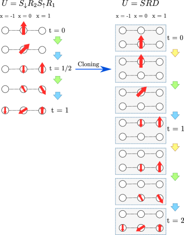
Figure 4: (Color online) Cloning of the split-step walk. Starting from the second clone, the state of the walker after $2t$ timesteps of the cloned walk is equivalent to the state of the original walker after $t$ timesteps.

In general, a state in the cloned system has the form

$$|{\psi}\rangle=\sum_{x}\sum_{s=\uparrow,\downarrow}\psi(x,s,1)|x,s,1\rangle+\psi(x,s,2)|{x,s,2}\rangle$$ (18)

The $\psi(\uparrow,2)$ and $\psi(\downarrow,1)$ components of the wavefunctions are unaffected by the shift operation $S$, while the $\psi(\uparrow,1)$ component is shifted one site to the right and $\psi(\downarrow,2)$ is shifted one site to the left (both these states are also shifted to the other clone). Thus we can divide the wavefunction into three parts,

$$\psi_{x}^{\uparrow} =\psi(x,\uparrow,1),$$ (19a)

$$\psi_{x}^{\downarrow} =\psi(x,\downarrow,2),$$ (19b)

$$\psi_{x}^{0} =(\psi(x,\downarrow,1)\,,\,\psi(x,\uparrow,2)).$$ (19c)

We then define the matrix $A$ to be the part of the timestep operator preceding the shift in the basis where the wavefunction is ordered as $\psi_{x}=(\psi_{x}^{\uparrow}\,,\,\psi_{x}^{\downarrow}\,,\,\psi_{x}^{0})$:

$$A\equiv RD=\begin{pmatrix}A^{\uparrow\uparrow}&A^{\uparrow\downarrow}&A^{\uparrow 0}\\ A^{\downarrow\uparrow}&A^{\downarrow\downarrow}&A^{\downarrow 0}\\ A^{0\uparrow}&A^{0\downarrow}&A^{00}\end{pmatrix}=\begin{pmatrix}A^{\uparrow}\\ A^{\downarrow}\\ A^{0}\end{pmatrix},$$ (20)

where we introduced $A^{mn}$ that maps from sector $n$ of the wavefunction to sector $m$, with $m,n\in\{\uparrow,\downarrow,0\}$, and $A^{m}\equiv(A^{m\uparrow},A^{m\downarrow},A^{m0})$. Each component depends on $x$.

The equation for the components of the scattering states can be written as

$$\begin{pmatrix}A_{x-1}^{\uparrow}\Psi_{x-1}^{\uparrow}\\ A_{x+1}^{\downarrow}\Psi_{x+1}^{\downarrow}\\ A_{x}^{0}\Psi_{x}^{0}\end{pmatrix}=e^{-i\varepsilon}\begin{pmatrix}\Psi_{x}^{\uparrow}\\ \Psi_{x}^{\downarrow}\\ \Psi_{x}^{0}\end{pmatrix},$$ (21)

where $\varepsilon=E/2$ is the quasienergy measured in the cloned system. The last component of Eq. (21) can be solved for $\psi_{x}^{0}$,

$$\Psi_{x}^{0}=G_{x}(\varepsilon)(A_{x}^{0\uparrow}\Psi_{x}^{\uparrow}+A_{x}^{0\downarrow}\Psi_{x}^{\downarrow}),$$ (22)

where we introduced the shorthand

$$G_{x}(\varepsilon)\equiv(e^{-i\varepsilon}1\!\!1_{2\times 2}-A_{x}^{00})^{-1}$$ (23)

for the resolvent of the matrix $A_{x}^{00}$. This enables us to relate $\Psi^{\uparrow}$ and $\Psi^{\downarrow}$ on adjacent sites.

III.2 Real-space scattering and transfer matrix

We arrive at what can be called the real-space scattering matrix from Eq. (21), using Eq. (22),

$$\begin{pmatrix}\Psi_{x-1}^{\downarrow}\\ \Psi_{x+1}^{\uparrow}\end{pmatrix}=\begin{pmatrix}\mathfrak{r}_{x}&\mathfrak{t}^{\prime}_{x}\\ \mathfrak{t}_{x}&\mathfrak{r}^{\prime}_{x}\end{pmatrix}\begin{pmatrix}\Psi_{x}^{\uparrow}\\ \Psi_{x}^{\downarrow}\end{pmatrix},$$ (24)

with the components of the above matrix defined as

$$\mathfrak{r}_{x} =e^{i\varepsilon}\left(A_{x}^{\downarrow\uparrow}+A_{x}^{\downarrow 0}G_{x}(\varepsilon)A_{x}^{0^{\uparrow}}\right);$$ (25a)

$$\mathfrak{t}_{x} =e^{i\varepsilon}\left(A_{x}^{\uparrow\uparrow}+A_{x}^{\uparrow 0}G_{x}(\varepsilon)A_{x}^{0^{\uparrow}}\right);$$ (25b)

$$\mathfrak{t}^{\prime}_{x} =e^{i\varepsilon}\left(A_{x}^{\downarrow\downarrow}+A_{x}^{\downarrow 0}G_{x}(\varepsilon)A_{x}^{0^{\downarrow}}\right);$$ (25c)

$$\mathfrak{r}^{\prime}_{x} =e^{i\varepsilon}\left(A_{x}^{\uparrow\downarrow}+A_{x}^{\uparrow 0}G_{x}(\varepsilon)A_{x}^{0^{\downarrow}}\right).$$ (25d)

We can interpret Eq. (24) in the following way: the components $\Psi_{x}^{\uparrow}$ and $\Psi_{x}^{\downarrow}$ act as incoming ”modes” that come to the site $x$ during a specific time step from the left/right respectively, while $\Psi_{x-1}^{\downarrow}$ and $\Psi_{x+1}^{\uparrow}$ act as outgoing modes towards the left/right from the same site. This justifies the name real-space scattering matrix for the matrix appearing in Eq. (24).

We can now obtain the reflection and transmission amplitudes that relate out- to ingoing plane waves in the two leads. First, we combine the $L$ individual $2\times 2$ real-space scattering matrices of the sites by the usual combination rule of scattering matrices, and thus get the real-space scattering matrix of the whole scattering region. From the components $\mathfrak{r}_{1,L}$ and $\mathfrak{t}_{1,L}$ of that matrix, the reflection and transmission amplitudes are given by the following formulas,

$$r(\varepsilon) =e^{i\varepsilon}\mathfrak{r}_{1,L};$$ (26a)

$$t(\varepsilon) =e^{i\varepsilon}\mathfrak{t}_{1,L}.$$ (26b)

The cloning of the system and the real-space scattering matrices give us a useful method for calculating scattering amplitudes and thus topological invariants both numerically and analytically. This method can be easily generalized to more complicated quantum walk protocols involving multiple shift and rotation operators, or larger number of internal states. Later, in Sect. V we will use it for the phase disordered split-step walk as well.

Although for numerical work, the real-space scattering matrix is a practical tool because of its numerical stability, for analytical formulas, the real-space transfer matrix $M_{x}$ is more useful. It is defined by the relation

$$\begin{pmatrix}\Psi_{x+1}^{\uparrow}\\ \Psi_{x}^{\downarrow}\end{pmatrix}=M_{x}\begin{pmatrix}\Psi_{x}^{\uparrow}\\ \Psi_{x-1}^{\downarrow}\end{pmatrix}$$ (27)

For the split-step walk, the real-space transfer matrix at quasienergy $E$ depends on the local angle parameters $\theta_{j}(x)$ through their sines and cosines, abbreviated as

$$s_{j} =\sin\theta_{j}(x); c_{j} =\cos\theta_{j}(x),$$ (28)

with $j=1,2$. The formula for the transfer matrix reads

$$M_{x}(E)=\frac{1}{c_{1}c_{2}}\cdot\\ \begin{pmatrix}e^{iE}+s_{1}s_{2}&-e^{-iE/2}s_{1}-e^{iE/2}s_{2}\\ -e^{iE/2}s_{1}-e^{-iE/2}s_{2}&-e^{-iE}+s_{1}s_{2}\end{pmatrix}.$$ (29)

III.3 Lyapunov exponents, topological invariants, and localization length of the disordered split-step quantum walk

To determine the topological invariants of the disordered split-step walk, we need the reflection amplitudes at quasienergies $0$ and $\pi$, as per Eq. (15). At these quasienergies, the real-space transfer matrix of a single site, Eq. (29), is considerably simplified,

$$M_{x}(0) =e^{\lambda_{x}(0)\sigma_{x}}$$ (30a)

$$M_{x}(\pi) =Ve^{\lambda_{x}(\pi)\sigma_{x}}V^{-1},$$ (30b)

where $V=V^{-1}=(\sigma_{x}-\sigma_{y})/\sqrt{2}$ is a $2\times 2$ unitary matrix. The parameters $\lambda_{x}(0)$ and $\lambda_{x}(\pi)$ are functions of the rotation angles $\theta_{1,2}(x)$ of the site,

$$\lambda_{x}(0)=\frac{1}{2}\text{ln}\,{\frac{(1-\sin\theta_{1}(x))(1-\sin\theta_{2}(x))}{(1+\sin{\theta_{1}(x)})(1+\sin{\theta_{2}(x)})}};$$ (31a)

$$\lambda_{x}(\pi)=\frac{1}{2}\text{ln}\,{\frac{(\sin{\theta_{1}(x)}-1)(1+\sin{\theta_{2}(x)})}{(1+\sin{\theta_{1}(x)})(\sin{\theta_{2}(x)}-1)}}.$$ (31b)

As seen from the Eqs. (30), at the quasienergies $E=0,\pi$ the real-space transfer matrices of the single sites all commute. Thus, the quantities $\lambda_{x}(0)$ and $\lambda_{x}(\pi)$ are additive: A system of $L$ consecutive sites is characterized by their sum, or equivalently, their average,

$$\lambda_{E} =\frac{1}{L}\sum_{x}\lambda_{x}(E)\qquad(E=0,\pi).$$ (32)

We will refer to this average $\lambda_{E}$ as the Lyapunov exponent.

The reflection and transmission amplitudes of the whole system at the relevant quasienergies are obtained from Eqs. (26a) using the Lyapunov exponents as

$$r(E) =-\tanh(L\lambda_{E});$$ (33a)

$$t(E) =1/\cosh(L\lambda_{E})\qquad\qquad(E=0,\pi).$$ (33b)

In the thermodynamical limit of $L\to\infty$, if the Lyapunov exponents are nonzero, the effective Hamiltonian of the quantum walk is an insulator, and $\left|{r(E)}\right|\to 1$. In that case, the topological invariants are obtained from Eq. (15),

$$\nu_{E}=-\frac{1}{2}\text{sign}(\lambda_{E}).$$ (34)

For a translation invariant system, the Lyapunov exponent is the same as the additive parameter of a single site, $\lambda_{E}=\lambda_{x}(E)$ as per Eq. (31). The topological invariants as a function of the global parameters $\theta_{1}$ and $\theta_{2}$, as read off from the plots of Fig. 5, agree with the previously known results of Fig. 2.

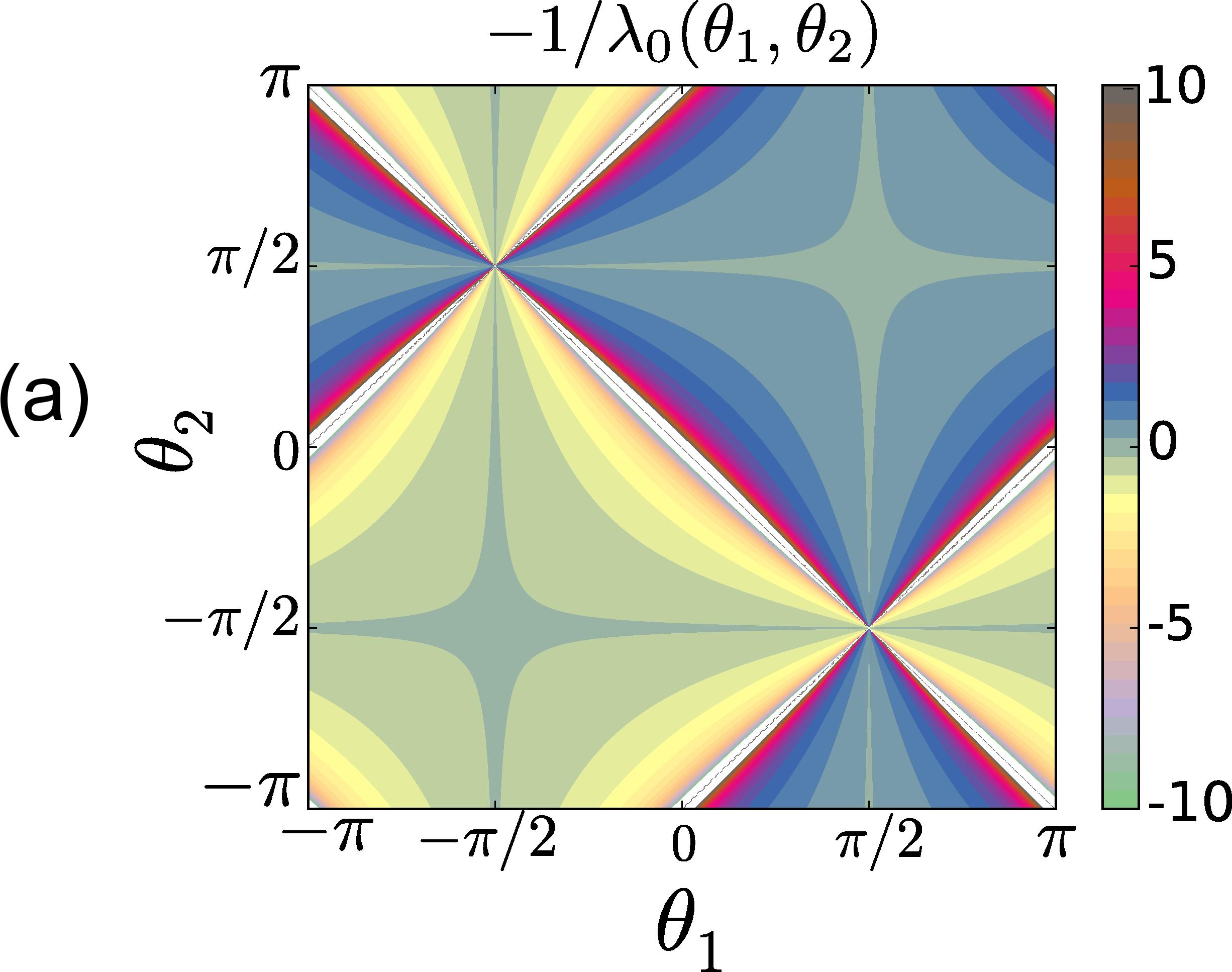
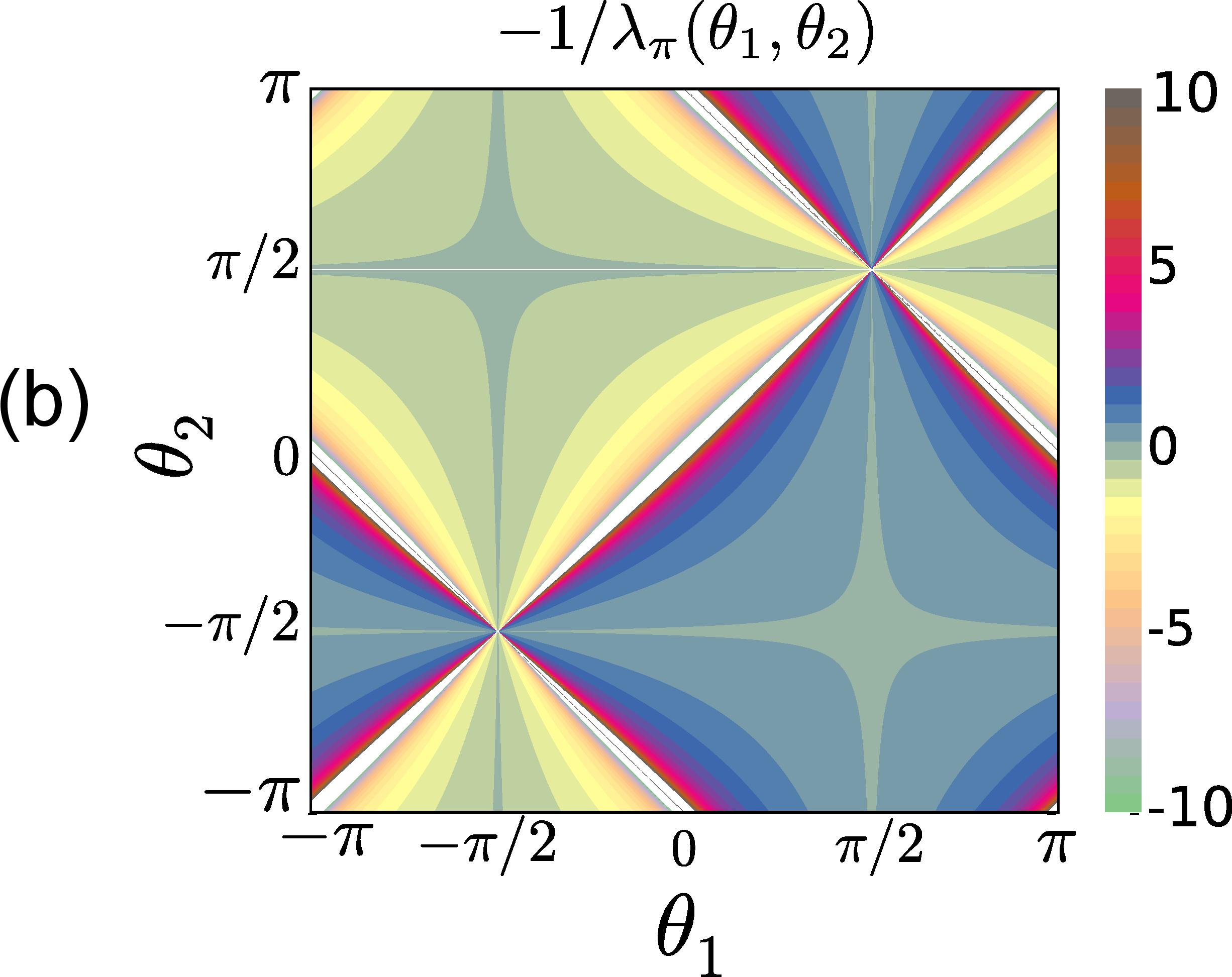
Figure 5: Color online) The negative inverse of the Lyapunov exponents, $-1/\lambda_{0}$ and $-1/\lambda_{\pi}$, as functions of the rotation angles $\theta_{1}$ and $\theta_{2}$, as described in Eqs. (31). Along the white lines, $\lambda_{E}\ll 1$, thus these points are on the topological phase boundary. Comparison with Fig. 2 shows that the signs of the Lyapunov exponents give the correct topological invariants as per Eq. (34).

While the signs of the Lyapunov exponents give us the two topological invariants, their absolute values tell us about the degree of localization of the states with quasienergies $E=0$ and $\pi$. To see this we define the quasienergy dependent localization length:

$$\xi(E)=-\frac{2L}{\text{ln}\,(|t(E)|^{2}/4)}$$ (35)

where it is assumed that the length of the scattering region is $L\to\infty$. From Eq. (33b) it follows, that for large $L$, the transmission amplitude at quasienergy $E=0$ or $\pi$ can be approximated by $t(E)\approx 2e^{-L|\lambda_{E}|}$. The localization length at these energies is therefore related to the Lyapunov exponent:

$$\xi(E)=1/|\lambda_{E}|\qquad(E=0,\pi)$$ (36)

Transmission at quasienergies $E=0,\pi$ decays exponentially with the system size whenever $\lambda_{E}\neq 0$. This shows that in any of the topological phases the quantum walk is insulating at both $E=0$ and $E=\pi$. On the phase boundary however, where $\lambda_{E}$ changes sign, $\xi(E)$ diverges and the walk is no longer insulating at one of these energies.

At $E=0$ and $\pi$, the localization length $\xi(E)$ also defines the characteristic size of the edge states. To see this, suppose that we have an interface between two bulks characterized by different Lyapunov exponents: $\lambda_{E}^{r}$ for $x\geq 1$, and $\lambda_{E}^{l}$ for $x\leq 0$. We want to study the existence of zero energy edge states localized near this interface. If we chose the components of the wavefunction $(\Psi_{1}^{\uparrow},\Psi_{0}^{\downarrow})$ at the interface to be an eigenstate of $\sigma_{x}$ with eigenvalue $\pm 1$, then according to Eq. (30), at $L\gg 1$ distance from the interface, the wavefunction will be proportional to $\exp(\pm L\lambda_{0}^{r})$ in the right bulk and $\exp(\mp L\lambda_{0}^{l})$ in the left bulk, as shown in Fig. 6. Since $\xi(0)=1/\lambda_{0}$, this indeed means that the edge state decays into the bulk with the characteristic length $\xi(0)$. Similar argument holds for $\pi$ energy edge states with an appropriate choice of boundary conditions at the interface. The above argument also shows that the bulk-boundary correspondence holds for the topological invariants defined in Eq. (34), since the only way to create normalized edge states is if the sign of the Lyapunov exponents is different in the two bulks.

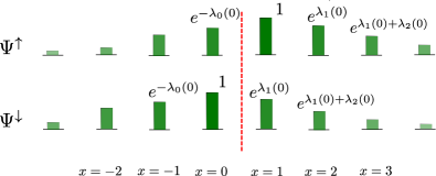
Figure 6: Example for the wavefunction of a zero-quasienergy edge state near the interface of two disordered bulks with differing topological invariants ($x<0:\lambda_{0}>0$ and $x>0:\lambda_{0}<0$). We chose $(\Psi_{1}^{\uparrow},\Psi_{0}^{\downarrow})$ to be $(1,1)$, thus the two components of the spinor wavefunction (upper row, lower row) are real and positive, and the wavefunction is not normalized to 1. The components of the wavefunction simply acquire factors of $e^{\pm|\lambda_{E}^{x}}|$ as we move away from the interface, so that the edge state decays exponentially into both bulks.

At a phase transition between different topological phases, at least one of the $\lambda_{E}$ changes its sign. Thus, as we approach the phase boundary, the corresponding characteristic length scale diverges and the states with quasienergy $E=0$ or $\pi$ that were previously localized become delocalized throughout the whole system, i.e., their support will scale with the system size $L$, which in turn leads to high values of transmission probability at these energies. This delocalized behaviour leads to a subdiffusive propagation of a walker started from the origin, as way previously noted in the case of the simple walk.Obuse and Kawakami (2011)

In the limit of infinite system length, we can write down exact formulas for the Lyapunov exponents even in the disordered case. As already stated, by disorder we mean a probability measure $\mu(\theta_{1},\theta_{2})$ given on the parameter space, according to which the angles $\theta_{1}$ and $\theta_{2}$ are chosen at each site. As we increase the length of the system, the sum $\sum_{x}\lambda_{x}(E)$ performs a random walk, with the coordinate $x$ playing the role of the time variable and $\lambda_{x}(E)$ playing the role of the distance covered in the $x$-th step. The two topological phases correspond to the cases when the random walk of the Lyapunov exponents drifts to the plus/minus infinity, where $\lambda_{E}$ can be thought of as a time-averaged drift velocity. For a system tuned to the topological phase boundary, the left and right drift terms cancel out and the random walk remains centered around the origin. Since the Lyapunov exponents are self-averaging, in the $L\rightarrow\infty$ limit, the ”time average” $\lambda_{E}$ becomes the ensemble average,

$$\lambda_{E}=\int\mathrm{d}\mu(\theta_{1},\theta_{2})\lambda_{x}(E,\theta_{1},\theta_{2})$$ (37)

According to Eq. (34), the sign of the above integral gives the topological invariant, while its absolute value defines the localization length as seen in Eq. (36) This means that Eq. (37), together with the definition of the Lyapunov exponents, Eq. (31), enables us to calculate the exact topological invariants and localization lengths for any disorder given in the form of $\mu(\theta_{1},\theta_{2})$. This is the main result of this paper.

IV Split-step walk with uniform disorder in the rotation angles

As an illustration of the ideas developed in the previous Section we calculate the topological phase map of the split-step walk with uniform disorder. We take the rotation angles $\theta_{1}$ and $\theta_{2}$ randomly and independently from a box distribution of width $W$ centered around mean values $\langle{\theta_{1}}\rangle,\langle{\theta_{2}}\rangle$. The corresponding probability density function,

$$\mu(\theta_{1},\theta_{2})=\frac{1}{4W^{2}}(\Theta(\langle\theta_{1}\rangle+W-\theta_{1})\cdot\Theta(\theta_{1}-\langle\theta_{1}\rangle+W))\\ \cdot(\Theta(\langle\theta_{2}\rangle+W-\theta_{2})\cdot\Theta(\theta_{2}-\langle\theta_{2}\rangle+W)),$$ (38)

is illustrated in Fig. 7. (For another illustrative example, that of binary disorder, see App. A.)

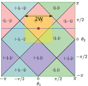
Figure 7: (Color online) The split-step walk with uniform disorder in the rotation angles. The parameters are taken from the yellow square of size $2W\times 2W$, with uniform probability. In Fig. 8 we move the middle of the distribution along the dashed line and vary the value of $W$ from $0$ to $\pi$.

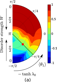
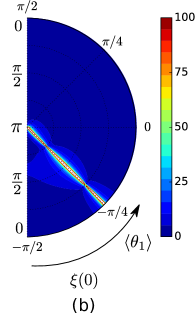
Figure 8: (Color online) Topological phase map of the split-step walk with $\langle\theta_{2}\rangle=\pi/4$ and uniform disorder in both rotation angles. The angle of the polar plot is the average $\langle\theta_{1}\rangle$ while disorder strength increases in the radial direction so that the middle of the circle corresponds to the strong disorder limit (see text). (a) Average reflection ampitude for a system consisting of a single site, $-\tanh{\lambda_{0}}$. The dashed line separates the two topological phases with $\nu_{0}=-1$ and $\nu_{0}=+1$, the (red) dot indicating the values of the parameters used in Fig. 10. (b) Localization length, computed for a system of infinite size. Along the phase boundary, the localization length $\xi(0)$ diverges.

In Fig. 8, we show the effects of disorder on the zero-quasienergy Lyapunov exponent, more precisely, on the average reflection amplitude for a system of size 1, and on the localization length. For simplicity, here we set the mean second rotation angle to $\langle{\theta_{2}}\rangle=\pi/4$, and we vary the mean of the first rotation angle, $\langle{\theta_{1}}\rangle$ from $-\pi/2$ to $\pi/2$ (along the dashed line in Fig. 7), as well as the disorder strength $W$. At each point in this phase map we numerically integrate Eq. (37) to obtain the Lyapunov exponent $\lambda_{0}$, and from it, the mean reflection amplitude $-\text{tanh}\,\lambda_{0}$ as well as the localization length at 0 quasienergy $\xi_{0}$. We find that the boundary between the two topological phases, where $\lambda_{0}=0$ (dashed line in Fig. 8), is at $\langle{\theta_{1}}\rangle=-\pi/4$, independent of the disorder $W$. Along this line, the system is critical, and the localization length diverges at quasienergy $E=0$.

IV.1 Disorder-induced delocalization

The system undergoes a disorder-induced delocalization transition in the strong disorder limit of $W=\pi$, where the rotation angles are taken from the whole parameter space with equal probabilites. At this limit, which corresponds to the central point in Fig. 8, we find analytically $\lambda_{0}=\lambda_{\pi}=0$. Thus, starting from a clean system, by increasing the strength of the disorder, we eventually reach a topological phase transition point, as shown in Fig. 9. This is accompanied by a delocalization of states with energies $E=0$ and $E=\pi$ as described in the previous section. Thus, while at small values of the disorder strength, the quantum walk is Anderson localized at all energies (we confirmed this separately by numerically calculating the localization lengths at other energies), strong disorder induces delocalization at the specific energies protected by the symmetries of the walk. This is similar to the case of the SSH modelMondragon-Shem et al. (2014). We note that the qualitative difference with respect to Ref. Mondragon-Shem et al., 2014, where in the infinite-disorder limit a transition to a trivial localized phase was found, in we checked that using different disorder for $\theta_{1}$ and $\theta_{2}$ leads to a transition from one topological phase to another, rather than delocalization.

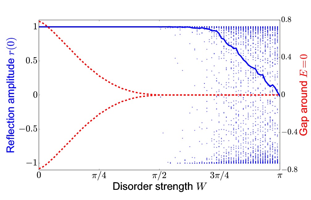
Figure 9: (Color online) Topological phase change as a result of increasing disorder, in a system of 200 sites, averaged over 1000 disorder realizations. Two branches of the dashed (red) curve: the highest/lowest quasienergy in the lower/upper band. The distance between the branches – the gap around zero quasienergy – gradually closes as disorder increases. Solid (blue) curve: the average zero quasienergy reflection amplitude. As the disorder increases, this remains quantized at $r(0)=1$ as necessitated by Eq. (15) long after the gap closes. As the disorder strength is increased even further, $\langle r(0)\rangle$ begins to change and eventually at $W=\pi$ it reaches $0$, signifying a phase transition point. The (blue) points represent $r(0)$ in the 1000 individual realizations whose average is the solid blue curve.

IV.2 No Anderson localization on the critical line

There are special cases for the split-step walk where disorder does not induce Anderson localization: if at some quasienergy the average Lyapunov exponent, defined by Eq. (37), vanishes. Uniform disorder in the rotation angles realizes such a special case if the quantum walk is on average on a phase boundary, i.e., if

$$\langle{\theta_{1}}\rangle=\pm\langle{\theta_{2}}\rangle+n\pi$$ (39)

for some $n\in\mathbb{Z}$, as seen in Fig. 7. In these cases, the localization length has to diverge at some critical quasienergy. As we show below, both the critical quasienergy and the shape of the divergence can be explained by a mapping to the disordered simple quantum walk.

Obuse and KawakamiObuse and Kawakami (2011) have found that the simple walk, defined in Eq. (8), with uniform disorder in the rotation angle $\theta$, does not undergo Anderson localization, no matter how strong the disorder is. A key part of their explanation is that apart from the chiral and particle-hole symmetries, the simple walk posesses a sublattice symmetry,

$$\Lambda U\Lambda =-U\qquad\Lambda=\sum_{\text{x even}}|{x}\rangle\langle{x}|-\sum_{\text{x odd}}|{x}\rangle\langle{x}|,$$ (40)

because the walker can only hop from even to odd sites or vice versa in one step. Using this extra symmetry, they argued (for more details, see Ref. Zhao and Gong, 2015), that Anderson localization is avoided because the localization length $\xi$ of the simple quantum walk diverges at $E=\pm\pi/2$, scaling as

$$\xi(E)=\xi_{0}|\log(\delta E\tau)|,$$ (41)

where $\delta E=E-E_{\text{crit}}$ is the distance from the critical quasienergy $E_{\text{crit}}=\pm\pi/2$, and $\tau$ is the mean free time. As illustrated in Fig. 10, the same effect occurs in split-step walks, if Eq. (39) is fulfilled. We show this explicitly in the rest of this section.

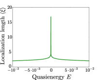
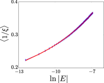
Figure 10: (Color online) Divergence of the localizaton length $\xi(E)$ as a function of quasienergy $E$ at a critical point with mean angles $\langle{\theta}\rangle_{1}=-\langle{\theta}\rangle_{2}=-\pi/4$ and disorder $W=\pi/2$ (see Fig. 8/(b)). (a) The average localization length diverges at $E=0$. (b) The scaling of the localization length near the critical energy. The dotted line indicates the curve (41) fitted to the numerical data, which gives $\tau=0.216$ and $\xi_{0}=0.322$. We used a system of 100 and 400 sites for figures (a) and (b) respectively. In both cases we averaged over 100 disorder realizations.

Using the sublattice symmetry property of Eq. (40), a split-step quantum walk can be understood as a doubled sequence of the simple quantum walk. Consider

$$\langle{x^{\prime},s^{\prime}}|[S_{\downarrow}R(\theta_{2})S_{\uparrow}R(\theta_{1})]^{t}|{x,s}\rangle=\\ \langle{2x^{\prime},s^{\prime}}|[SR(\theta^{\prime})SR(\theta^{\prime})]^{t}|{2x,s}\rangle,$$ (42)

with the position dependent rotation angles $\theta^{\prime}(x)$ defined by the relations

$$\theta^{\prime}(2x) =\theta_{1}(x);$$ (43)

$$\theta^{\prime}(2x-1) =\theta_{2}(x).$$ (44)

This mapping is closely related to that used in Ref. Asboth and Edge, 2015 to realize a split-step quantum walk as a periodically driven Hamiltonian.

The mapping of Eq. (42) shows that if $\langle{\theta_{1}}\rangle=\langle{\theta_{2}}\rangle$, the correlation length of the split-step walk has to diverge at quasienergy $E_{\text{crit}}=\pi$ following the scaling of Eq. (41). By Eq. (42), two timesteps of a simple quantum walk with angle $\theta$ can be understood as a single timestep of a split-step quantum walk with $\theta_{1}=\theta_{2}=\theta$. The introduction of uncorrelated box disorder in the rotation angle $\theta$ of the simple quantum walk translates to uniform disorder in the angles $\theta_{1}$ and $\theta_{2}$ of the quantum walk, with $\langle{\theta_{1}}\rangle=\langle{\theta_{2}}\rangle$. The doubling of the timestep moves the critical quasienergy from $\pm\pi/2$ to $\pm\pi$.

A mapping between different split-step quantum walks shows that if $\langle{\theta_{1}}\rangle=\langle{\theta_{2}}\rangle\pm\pi$, the divergence of the localization length follows the same functional form of Eq. (41), with $E_{\text{crit}}=0$. Changing $\theta_{j}(x)\to\theta_{j}(x)\pm\pi$ for all $x$, for either $j=1$ or $j=2$, results in an overall factor of $-1$ for the timestep operator $U$. This shifts the divergence of the localization length of the quantum walk by $\pi$, to $E_{\text{crit}}=0$.

A mapping between the transfer matrices of different split-step quantum walks shows that if $\langle{\theta_{1}}\rangle=-\langle{\theta_{2}}\rangle+n\pi$, the localization length diverges according to Eq. (41), with shifted $E_{\text{crit}}$. According to Eq. (29), changing either $\theta_{1}(x)$ to $-\theta_{1}(x)$ or $\theta_{2}(x)$ to $-\theta_{2}(x)$ changes the transfer matrix $M_{x}$ at $x$ to $M_{x}^{\prime}$, with

$$M_{x}^{\prime}(E+\pi)=-\begin{pmatrix}i&0\\ 0&1\end{pmatrix}M_{x}(E)\begin{pmatrix}-i&0\\ 0&1\end{pmatrix}.$$ (45)

The transfer matrix $M_{x}^{\prime}(E+\pi)$ is a unitary transform of $M_{x}(E)$, up to the unimportant factor of $-1$. Since the transformation is independent of $x$, the Lyapunov exponents at $E$ of the original walk are equal to those of the transformed walk at $E+\pi$. This shows that if $\langle{\theta_{1}}\rangle=-\langle{\theta_{2}}\rangle$, the localization length diverges at $E_{\text{crit}}=0$, while if $\langle{\theta_{1}}\rangle=-\langle{\theta_{2}}\rangle\pm\pi$, it diverges at $E_{\text{crit}}=\pi$, following the scaling of Eq. (41).

Our results also shed new light on the absence of Anderson localization in the simple quantum walkObuse and Kawakami (2011). As we have shown, the simple quantum walk with disorder in the rotation angles is not Anderson localized because it constitutes a disordered split-step quantum walk tuned to a topological phase transition point.

V Split-step walk with phase disorder

We now consider the phase disordered split-step walk, introduced in Eq. (9). Since phase disorder breaks both chiral and particle-hole symmetry, we expect that it induces Anderson localization at all quasienergies. There is a way, however, to add phase disorder to the split-step walk and keep chiral symmetry: in that case, we expect to see localization-delocalization transitions as with angle disorder in the previous Section. We discuss both types of phase disorder, and illustrate our results by numerical examples that can be compared directly with those on angle disorder of the previous Section.

The simplest way to introduce phase disorder is to multiply the wavefunction of the walker at the end of each timestep by a position- and spin-dependent phase factor $\phi(x,s)$, chosen randomly and independently at each site, as defined in Eq. (9). For the examples in this section we used an extra restriction of $\phi(x,\uparrow)=-\phi(x,\downarrow)$, whereby the phase operator reads

$$P(\phi)=\sum_{x}|x\rangle\langle x|\otimes e^{-i\phi(x)\sigma_{z}},$$ (46)

with the phase chosen from an interval $[-\Delta\phi,\Delta\phi]$ with uniform distribution. Just as with the more general phase disorder, due to this extra operation, both particle-hole symmetry and chiral symmetry of the quantum walk are broken. Thus, in the presence of phase disorder, there are no localization-delocalization transitions.

To highlight the role of chiral symmetry, we also consider adding phase disorder to the split-step walk in a chiral symmetric way. This requires two phase operators per timestep,

$$U^{\prime}(\phi,\theta_{1},\theta_{2})=P(\phi)S_{\downarrow}R(\theta_{2})S_{\uparrow}P(\phi)R(\theta_{1}).$$ (47)

The second phase operation restores chiral symmetry since $\sigma_{x}P(\phi)\sigma_{x}=P(\phi)^{-1}$. Repeating the calculation of the real-space transfer matrix, Eq. (29), with $R(\theta_{1})$ replaced by $P(\phi)R(\theta_{1})P(\phi)$, we find that this matrix is just multiplied by a factor of $e^{2i\phi(x)}$. For example at zero quasienergy,

$$M_{x}(0)=e^{2i\phi(x)}e^{\lambda_{x}(0)\sigma_{x}},$$ (48)

and similarly for $E=\pi$. The extra phase factor drops out from both the reflection amplitude and the localization length so that the description we gave in the previous section is unaffected.

To show the effects of phase disorder numerically, we have calculated the localization lengths $\xi$ for a range of angle disorders and phase disorders, shown in Fig. 11. For easy comparison with the results of the previous Section, Fig. 8, we fix $\langle{\theta_{2}}\rangle=\pi/4$, and show the localization length $\xi(0)$ as a function of the mean first rotation angle $\langle{\theta_{1}}\rangle$ and of disorder, introduced in equal measures to both rotation angles and to the phases $\phi$, setting $W=\Delta\phi$. Thus, the perimeter of the plot of Fig. 11, with $W=0$, corresponds to the perimeter of the plots of Fig. 8b). As expected, symmetry breaking phase disorder, Fig. 11a), destroys the delocalization transition and for large values of $\Delta\phi$, the states with $0$ quasienergy are localized for all parameters. Phase disorder that respects chiral symmetry, Fig. 11(b), however, has the numerically obtained localization lengths taking large values at $\langle{\theta_{1}}\rangle=-\pi/4$, which is the phase boundary between topological phases, and where the theory (shown in Fig. 8) predicts divergences.

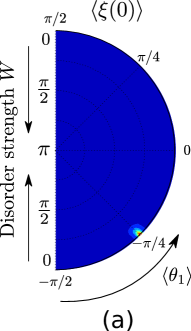
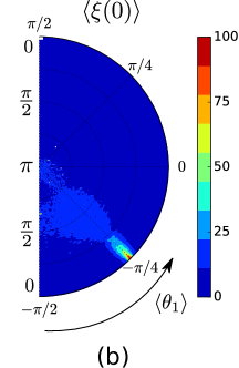
Figure 11: (Color online) Average localization lengths at quasienergy $E=0$ for phase disordered quantum walks with equal disorder strengths for the rotation angles and the random phases, $\Delta\phi=W$. (a) Single phase shift. The timestep operator is $U=P(\phi)S_{\downarrow}R(\theta_{2})S_{\uparrow}R(\theta_{1})$ thus chiral symmetry is broken. (b) Double phase shift, with timestep $U^{\prime}=P(\phi)S_{\downarrow}R(\theta_{2})S_{\uparrow}P(\phi)R(\theta_{1})$, exhibiting chiral symmetry. Single phase disorder leads to topological triviality and causes all states to be localized while double phase disorder restores the phase map seen in Fig. 7 with a delocalization transition at the topological phase border. The localization lengths were calculated using a system of $80$ sites and averaged over $100$ realizations.

We also show the effects of symmetry breaking and of chiral symmetric phase disorder on the time evolution of the split-step quantum walk directly in Fig. 12. Here we show the position variance of a particle started from the origin after $t$ timesteps,

$$\text{var}(x)=\langle{\psi(t)}|x^{2}|{\psi(t)}\rangle-[\langle{\psi(t)}|x|{\psi(t)}\rangle]^{2}.$$ (49)

We used the strong disorder limit in the rotation angles, $W=\pi$, and used phase disorder with amplitude $\Delta\phi=\pi/4$. For a single phase shift (symmetry breaking phase disorder), the walker is localized and $\text{var}(x)\rightarrow\text{constant}$ for large $t$. However, in the double phase shift case, when chiral symmetry is restored, we see the subdiffusive bevaviour discussed in the previous Section, with the walker slowly spreading through the system. These results are in accordance with those from the localization lengths.

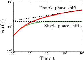
Figure 12: (Color online) Variance of the position of a quantum walker started from a single site as a function of time for single and double phase disorder, averaged over 10000 disorder realizations, with angle disorder strength $W=\pi$ and phase disorder strength $\Delta\phi=\pi/4$. For a timestep containing a single phase shift (green thin curve), the walker is localized and the variance tends to a constant, while for the chiral symmetric case defined in Eq. (47) (red thick curve), the walker spreads subdiffusively. In both cases, we fitted the function $\text{var}(x)=a\cdot t^{b}$ to the data points with $t>1000$ and found that the exponent $b$ is $9,57\cdot 10^{-4}$ in the first and $0,107$ in the second case. The dashed lines show the fitted curves.

VI Conclusions

We considered the effects of disorder on the localization properties and on topological phases of the one-dimensional split-step quantum walk. We introduced an effective numerical tool (the cloning trick), which allowed us to calculate the scattering amplitudes for the split-step walk and efficiently calculate the topological invariants proposed in Ref. Tarasinski et al., 2014. We then showed theoretically and investigated numerically various localization-delocalization transitions that occur whenever this system is tuned to a critical point at a topological phase transition. We have shown using a mapping that the subdiffusive spreading of the simple quantum walk with angle disorderObuse and Kawakami (2011) can be understood in this framework. We have shown that angle disorder generically localizes the split-step quantum walk, but that complete disorder in the rotation angles places it in a critical state with subdiffusive instead of localized dynamics. Finally, we illustrated the importance of symmetries on localization-delocalization through the example of phase disorder.

It is interesting to compare our results on the one-dimensional split-step quantum walk (1D) with those obtained in Ref. Edge and Asboth, 2015 regarding the two-dimensional split-step quantum walk (2D). In the 2D case, the topological phases did not require any symmetry of the system, and so phase disorder did not destroy the topological phase. Similarly to angle disorder in the 1D case, phase disorder in the 2D case was found to lead to Anderson localization, except when the system was tuned to criticality (as in the case of the Hadamard walk). The disorder-induced delocalization transition however was reached in both the 1D and the 2D case by using complete disorder in the rotation angles. In the 2D case, it was found that angle disorder alone does not lead to Anderson localization, possibly related to the presence of particle-hole symmetry. The effect of particle-hole symmetric disorder remains to be studied in the 1D case.

Our results show how the understanding of topological phases of quantum walks can help interpret their behaviour under different types of disorder. This could be important to identify which types of quantum walks are practical for information processing purposes, and which types of disorder it is crucial to supress in such applications.

Appendix A Split-step walk with binary disorder

In the main text we used uniform disorder as an illustration of the general formalism. In this section we present another simple example that can be treated analytically and is useful to obtain intuition regarding the disordered quantum walk. Consider a split-step quantum walk where the rotation angles $\theta_{1}$ and $\theta_{2}$ can take two different values: $\theta_{1}^{A}$, $\theta_{2}^{A}$ or $\theta_{1}^{B}$, $\theta_{2}^{B}$. At each site, we chose one of these two set of values, with probabilities $q$ and $1-q$, so that the corresponding probability measure is

$$\mu(\theta_{1},\theta_{2})=q\,\delta(\theta_{1}-\theta_{1}^{A})\delta(\theta_{2}-\theta_{2}^{A})\\ +(1-q)\,\delta(\theta_{1}-\theta_{1}^{B})\delta(\theta_{2}-\theta_{2}^{B}).$$ (50)

We fix the point $A$ in parameter space as

$$\theta_{1}^{A} =0.625\pi; \theta_{2}^{A} =-0.125\pi,$$ (51)

and choose point $B$ to lie on a straight line that is parallel to one of the phase borders and goes through point $A$,

$$\theta_{1}^{B} =\theta_{1}^{A}-m\;\pi; \theta_{2}^{B} =\theta_{2}^{A}+m\;\pi,$$ (52)

where the parameter $m\in[0,1]$ measures the distance between points $A$ and $B$ in parameter space as shown in Fig. 13. When $m=0$, the two points coincide while $m=1$ corresponds to the case when their distance is maximal.

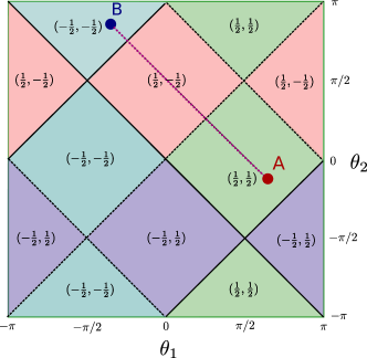
Figure 13: (Color online) Split-step walk with binary disorder. The red and blue dots represent points $A$ and $B$ in the case $m=1$, while the dashed line shows the possible values of $B$, while $m$ goes from $0$ to $1$.

At $m=3/8$, the point $B$ crosses the line where the gap at $E=\pi$ closes and the invariant $\nu_{\pi}$ changes. Thus, for values $m>3/8$ the two limits $q=0$ and $q=1$ belong to two different topological phases. We want to find the exact value $q_{\text{crit}}$ for each $m$ where the phase transition occurs. Suppose that we have a number of $L_{A}$ sites with parameters $\theta_{1,2}^{A}$ in our system and a number of $L_{B}$ sites from the point $B$. The condition for the phase transition can then by written as

$$\lambda_{E}=L_{A}\lambda_{E}^{A}+L_{B}\lambda_{E}^{B}=0.$$ (53)

From this we acquire the critical value of the mixing probability $q$,

$$q_{\text{crit}}=\frac{1}{1+\frac{L_{B}}{L_{A}}}=\frac{1}{1-\frac{\lambda^{A}}{\lambda^{B}}}.$$ (54)

The critical line $q_{\text{crit}}(m)$ for $E=\pi$ is shown in Fig. 14 along with the numerically calculated average reflection amplitudes at quasienergy $\pi$.

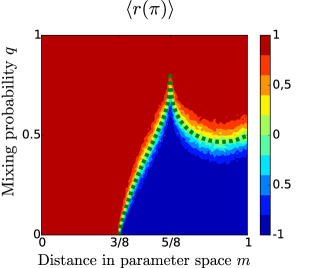
Figure 14: (Color online) Topological phases of the split-step walk with binary disorder. Color coding shows the reflection amplitudes at $E=\pi$ for a system of $40$ sites averaged over $100$ samples. The green dashed line shows the critical mixing probability $q_{\text{crit}}$ calculated using Eq. (54). The peak at $m=5/8$ corresponds the the case when the point $B$ is in the middle of a topological phases and $\lambda_{\pi}$ diverges.

This binary disordered model, while somewhat unphysical, shows the importance of the Lyapunov exponents defined in Eqs. (30). They serve as weight factors, determining how much a given site contributes to the overall topoogical invariants of the whole system.

Appendix B Critical exponent for uniform disorder

In this section we will give the critical exponent with which the localization length $\xi(0)$ or $\xi(\pi)$ diverges when we approach the topological phase boundary in parameter space. There is also a different critical exponent when we are at a phase boundary: then the function $\xi(E)$ diverges as the quasienergy approaches $0$ (or $\pi$). This was discussed in section IV of the main text.

Let us first look at the clean case. Near the phase boundary $\theta_{1}=-\theta_{2}$ we can expand the function $\lambda_{0}$ in the small parameter $\delta=\theta_{1}+\theta_{2}$. From the definition Eq. (31) we get that $\lambda_{0}\propto\delta$ so that $\xi(0)\propto\delta^{-1}$. This means that in the clean system the critical exponent is $\nu=-1$.

When uniform disorder is applied, we can approach the phase boundary in two different ways as shown in Fig. 8: either by changing the average values the rotation angles (similarly to the clean case) or by increasing the disorder strength until we reach the strong disorder limit as described in the main text. Numerical evaluation of the integral (37) in the vicinity of the phase boundary verifies that the critical exponent remains $\nu=-1$ in both cases as seen in Fig. 15.

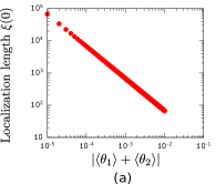
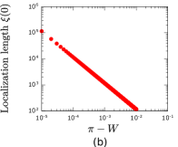
Figure 15: Behavior of the localization length $\xi(0)$ near the topological phase boundary. (a) Split-step walk with uniform disorder, disorder strength set to $W=0.1\pi$. The average rotation angles approach the gap closing line $\theta_{1}+\theta_{2}=0$. (b) Near the strong disorder limit, $W\approx\pi$. In both cases, we found a critical exponent $\nu=-1$.

Appendix C Comparison with the real-space winding number method

As we mentioned in the main text, there is an alternative way to calculate topological invariants for a disordered system, apart from the scattering matrix approach that we used to study the split-step walk. This other approach, based on non-commutative geometry tools, was used to study two dimensional topological insulators at strong disorderProdan (2011), and, more recently, the disordered SSH modelMondragon-Shem et al. (2014). In this formalism, the winding number of a one dimensional topological insulator with only two bands can be calculated by the expression

$$\nu=-Tr(Q_{-+}[X,Q_{+-}])/L,$$ (55)

where $X$ is the position operator, $Q_{-+}=\Gamma_{-}Q\Gamma_{+}$ and $Q_{+-}=\Gamma_{+}Q\Gamma_{-}$, with $Q$ being the flat band version of the Hamiltonian $H$, defined by replacing each eigenvalue of $H$ with its sign: $Q=\text{sign}(H)$. The operators $\Gamma_{+}$ and $\Gamma_{-}$ are the projectors associated to the chiral symmetry operator $\Gamma$ by $\Gamma=\Gamma_{+}-\Gamma_{-}$.

Evaluation of the winding number, Eq. (55), for a finite size system with periodic boundary conditions requires non-trivial approximations as described in Prodan’s paperProdan (2011). In this case, the resolution in quasimomentum space for a system of $L$ sites is given by $\Delta=2\pi/L$. We approximate the differential $\partial_{k}A(k)$ for some function $A(k)$ of the quasimomenta with discrete differences in the following way:

$$\partial_{k}A(k)\rightarrow\delta_{k}A(k_{n})=\sum_{m=1}^{q}c_{m}[A(k_{n}+m\Delta)-A(k_{n}-m\Delta)],$$ (56)

where $q$ is of order $L/2$.

If we assume that $A(k)$ can be expressed as a Fourier series, then it is enough to find the coefficients $c_{m}$ that give a good approximation for functions of the form $e^{ikx}$. For these, the formula (56) gives

$$(\partial_{k}-\delta_{k})e^{ikx}=i(x-2\sum_{m}c_{m}\sin(m\Delta x))e^{ikx}.$$ (57)

We can make the above expression disappear in the first $2q-1$ orders of $\Delta x$ by choosing $c_{m}$ to be the solutions of the equation

$$\bm{M}\bm{c}^{T}=\frac{1}{2\Delta}(1,0,0,\dots,0)^{T};\\ M_{nm}=m^{2n-1}\qquad n,m=1,\dots,Q.$$ (58)

In this case, $(\partial_{k}-\delta_{k})e^{ikx}=~{}\mathcal{O}(\Delta^{2q-1})$. By choosing $q=L/2$ we can make the error of the approximation to be of order $~{}\mathcal{O}(\Delta^{L-1})$.

For the split-step walk, Eq. (55) can be used in both chiral symmetric timeframes defined in Eqs. (10) and (11). This gives us two winding numbers $\nu^{\prime}$ and $\nu^{\prime\prime}$. The topological invariants are given as combinations of these twoAsbóth and Obuse (2013):

$$\nu_{0} =\frac{\nu^{\prime}+\nu^{\prime\prime}}{2};$$ (59a)

$$\nu_{\pi} =\frac{\nu^{\prime}-\nu^{\prime\prime}}{2}.$$ (59b)

These equations, along with Eq. (55) enable us to calculate the topological invariants numerically. Below, in Fig. 16 we show the results for $\nu_{0}$, along with those performed using the scattering matrices described in the main text. The two methods yield the same results qualitatively. However, we note that while the reflection amplitude of the finite system remains close to the value it has in the thermodynamic limit even for relatively strong disorder, the real-space winding number is more easily affected by numerucal inaccuracies resulting from small system sites. The scattering matrix method is also more efficient numerically (it scales linearly with the system size).

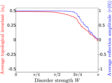
Figure 16: (Color online) For a disordered quantum walk, the bulk winding number (solid red) and the average reflection amplitude (dashed blue) give similar predictions about the topological phase. We used a system of 100 sites and averaged over 1000 disorder realizations. For the bulk winding number, Eqs. (55) were used, while the reflection amplitude was obtained by iterating the scattering matrix.