Nondestructive verification of continuous-variable entanglement

Abstract

An optical procedure in the context of continuous variables to verify bipartite entanglement without destroying both systems and their entanglement is proposed. To perform the nondestructive verification of entanglement, the method relies on beam-splitter and quantum nondemolition (QND) interactions of the signal modes with two ancillary probe modes. The probe modes are measured by homodyne detections, and the obtained information is used to feedforward modulation of signal modes, concluding the procedure. Characterizing the method by figures of merit used in QND processes, we can establish the conditions for an effectively quantum scheme. Based on such conditions, it is shown that the classical information acquired from the homodyne detections of probe modes is sufficient to verify the entanglement of the output signal modes. The processing impact due to added noise on the output entanglement is assessed in the case of Gaussian modes.

I Introduction

Entanglement is one of the most fundamental resources for performing processes in quantum information and computation. Besides the technological possibilities, the entanglement challenges our understanding of the quantum world and its connection with classical physics Nielsen ; Horodecki09 ; Kimble . Recently, many experiments have accomplished quantum communication protocols sending light signals over distances of hundreds of kilometers Yin12 ; Ma12 ; Inagaki13 . In these experiments, the entanglement was an essential part. It has also been studied as the use of entangled signals over long distances may increase the applicability of quantum cryptography protocols Scheidl09 . Thus it is very natural to devise stages along the transmission of entangled signals that verify if such signals are really entangled, without destroying or excessively disturbing them during the verification processes. In other words, for future quantum communications, nondestructive certification protocols of entanglement will be required, ensuring the use of entanglement for subsequent processes of quantum information. Studies of nondestructive entanglement verification or analysis have been done in the framework of discrete variable systems, such as single photons Barrett05 ; Tang12 ; Liu16 .

Differently from the previously cited studies, quantum communications using entangled signals may also be carried out in the context of continuous-variable systems, e. g., bright beams. The light beams may be regarded as oscillation modes, such that the states are vectors of an infinite-dimensional Hilbert space and observables are continuous spectrum operators, analogously to the position and momentum operators of the quantum harmonic oscillator Braunstein05 . For light beams, we consider amplitude and phase operators, also called quadratures. The research field of continuous-variable systems is very active and has extensive literature. Examples of quantum information protocols performed with continuous-variable light modes are quantum teleportation Braunstein98 ; Furusawa98 ; Bowen03 ; Zhang03 , cloning Buzek96 ; Grover/Cirac99 ; Andersen05 , and telecloning Murao99 ; Loock01 ; Koike06 . In such cases, the entanglement is an essential ingredient, therefore its conservation and its verification are primordial to further more complex applications.

Thus a minimally invasive measurement method to observe the entanglement is desirable. Although all quantum measurement entails a back-action effect, we can measure the signal, in order to preserve some of the properties of its original state. In particular, a quantum nondemolition (QND) measurement is able to measure an observable without disturbing it, at the expense of a back-action disturbance on the conjugate observable Braginsky80 ; Braginsky96 ; Grangier98 ; Wiseman-Milburn . In quantum optics, the QND measurements were initially performed by coupling the signal and probe modes in nonlinear optical media, such as Kerr media, optical fibers (third-order nonlinearity) Milburn83 ; Imoto85 ; Levenson86 , and in optical parametric amplifiers (second-order nonlinearity) Yurke85 ; La Porta89 . Other proposals relied on feedforward modulation of signal modes and off-line squeezed probe modes Buchler99 ; Andersen02 ; Filip05 ; Yoshikawa08 , in which it is not necessary to strongly pump a nonlinear medium in line to the signal modes. The combination of off-line squeezed probe modes, linear optics, homodyne detection, and feedforward loop has inspired many other optical operations, such as squeezing Filip05 ; Buchler01 ; Yoshikawa07 ; Miyata14 , implementation of the one-way computation Ukai11 ; Yokoyama15 , realization of third-order nonlinear operation Marek11 , and other varieties of QND interactions Marek10 ; Yokoyama14 .

In this paper we propose a nondestructive method to verify continuous-variable bipartite entanglement, which uses QND and beam-splitter interactions between the signal modes and two other probe modes. After the interactions, the probe modes are measured by homodyne detections, so that the obtained photocurrents serve both to calculate the entanglement condition, so as to modulate the signal modes by electro-optic feedforward modulation, as has been implemented in noiseless optical amplifiers Ralph97 ; Lam97 ; Huntington98 . The proposed scheme has the benefit of not mixing up the output signal modes to each other, which would change the global properties of entanglement Simon ; DGCZ . Another relevant result is that the obtained entanglement condition is valid to the output signals, ensuring the quantum correlation properties resulting from the process. The cost of the procedure, manageable by the scheme parameters, is the addition of excess uncorrelated noise in both signal modes.

This paper is organized as follows. In Section II, we describe the entanglement verification procedure, in which is shown the quadrature transformations of the signal and probe modes, in each stage of the scheme. In Section III, we characterize the procedure by the well-known QND measurement criteria. In Section IV, based on the results of the previous section, we present how we compute a sufficient entanglement condition to the two output signal modes, by detecting both probe modes. The effects of the noise addition on the signal entanglement are assessed in Section V, where the entanglement degradation is obtained in the case of Gaussian systems. Finally, we discuss the results and possibilities of this scheme in Section VI.

II Entanglement verification

The goal of the process is to verify if a pair of signal modes are entangled without destroying them. Since we consider the signal modes as continuous-variable systems, we write their input quadrature operators as $\hat{x}_{1}$ and $\hat{p}_{1}$ for mode 1 and $\hat{x}_{2}$ and $\hat{p}_{2}$ for mode 2. In order to carry out the entanglement verification, two independent auxiliary beams must be introduced, characterized with input quadrature operators $\hat{x}_{A}$ and $\hat{p}_{A}$ for mode A, and $\hat{x}_{B}$ and $\hat{p}_{B}$ for mode B. All operators obey the usual commutation relations, $[\hat{x}_{i},\hat{p}_{j}]=i\delta_{ij}$, for $\{i;j\}=\{1;2;A;B\}$ Braunstein05 . The auxiliary beams are used as probe modes, interacting with the signal modes and after measured by homodyne detections. Thus, the states of these probe modes A and B must be previously known. Following the theoretical proposals of previous articles Buchler99 ; Andersen02 ; Filip05 , the probe modes must be prepared in strongly squeezed vacuum states. In what follows, the squeezed quadratures of the probe modes are related to the operators $\hat{p}_{A}$ and $\hat{x}_{B}$. First, each signal mode is coupled to each probe mode by ideal QND interactions. Interactions such as these have been performed by coupling beams in nonlinear optical media (see Grangier98 and citations therein). However QND interactions were also performed using only linear optics, an auxiliary squeezed beam, homodyne detection, and feedforward modulation Filip05 ; Yoshikawa08 . As illustrated in Figure 1, the beam pairs (1, A) and (2, B) are coupled by QND interactions, such that for modes 1 and A, with gain $G_{1}$:

$$\hat{x}_{1}^{\prime} = \hat{x}_{1},$$ (1)

$$\hat{p}_{1}^{\prime} = \hat{p}_{1}-G_{1}\hat{p}_{A},$$ (2)

$$\hat{x}_{A}^{\prime} = \hat{x}_{A}+G_{1}\hat{x}_{1},$$ (3)

$$\hat{p}_{A}^{\prime} = \hat{p}_{A},$$ (4)

and for modes 2 and B, with gain $G_{2}$:

$$\hat{x}_{2}^{\prime} = \hat{x}_{2}+G_{2}\hat{x}_{B},$$ (5)

$$\hat{p}_{2}^{\prime} = \hat{p}_{2},$$ (6)

$$\hat{x}_{B}^{\prime} = \hat{x}_{B},$$ (7)

$$\hat{p}_{B}^{\prime} = \hat{p}_{B}-G_{2}\hat{p}_{2}.$$ (8)

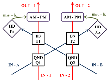
Figure 1: Schematic setup for the entanglement verification of modes 1 and 2. The probe modes are modes A and B. HD: homodyne detection for quadrature operators $\hat{x}_{A}$ and $\hat{p}_{B}$; BS: beam-splitter coupling with transmittances $T_{1}$ and $T_{2}$; QND: quantum nondemolition coupling with gains $Q_{1}$ and $Q_{2}$; AM-PM: feedforward modulators. $m_{x_{A}}$ and $m_{p_{B}}$ are the photocurrents obtained in detectors. These signals are used in both the feedforward process and to compute the entanglement condition.

After these first two QND interactions, the modes interact again, crossing probe modes with signal modes. Both interactions operate as beam splitters with transmittance $T_{1}$ for modes 1 and B and transmittance $T_{2}$ for modes 2 and A. Thus from equations (1)-(8), we have to modes 1 and B:

$$\hat{x}_{1}^{\prime\prime} = \sqrt{T_{1}}\hat{x}_{1}-\sqrt{1-T_{1}}\hat{x}_{B},$$ (9)

$$\hat{p}_{1}^{\prime\prime} = \sqrt{T_{1}}(\hat{p}_{1}-G_{1}\hat{p}_{A})-\sqrt{1-T_{1}}(\hat{p}_{B}-G_{2}\hat{p}_{2}),$$ (10)

$$\hat{x}_{B}^{\prime\prime} = \sqrt{T_{1}}\hat{x}_{B}+\sqrt{1-T_{1}}\hat{x}_{1},$$ (11)

$$\hat{p}_{B}^{\prime\prime} = \sqrt{T_{1}}(\hat{p}_{B}-G_{2}\hat{p}_{2})+\sqrt{1-T_{1}}(\hat{p}_{1}-G_{1}\hat{p}_{A}),$$ (12)

and to modes 2 and A:

$$\hat{x}_{2}^{\prime\prime} = \sqrt{T_{2}}(\hat{x}_{2}+G_{2}\hat{x}_{B})-\sqrt{1-T_{2}}(\hat{x}_{A}+G_{1}\hat{x}_{1}),$$ (13)

$$\hat{p}_{2}^{\prime\prime} = \sqrt{T_{2}}\hat{p}_{2}-\sqrt{1-T_{2}}\hat{p}_{A},$$ (14)

$$\hat{x}_{A}^{\prime\prime} = \sqrt{T_{2}}(\hat{x}_{A}+G_{1}\hat{x}_{1})+\sqrt{1-T_{2}}(\hat{x}_{2}+G_{2}\hat{x}_{B}),$$ (15)

$$\hat{p}_{A}^{\prime\prime} = \sqrt{T_{2}}\hat{p}_{A}+\sqrt{1-T_{2}}\hat{p}_{2}.$$ (16)

These first two steps are necessary for the probe modes to obtain sufficient information from the signal modes. Then the probe modes are measured by homodyne detection processes, providing classical signals (photocurrents) sufficient to compute and verify if the signal modes are entangled. However, as we see in equations (9), (10), (13) and (14), the signal modes are affected by interactions. These perturbations can be corrected a posteriori with feedforward modulations, using phase and amplitude electro-optic modulators. Setting up the local oscillators of the homodyne detections, we select the quadratures $\hat{x}_{A}^{\prime\prime}$ and $\hat{p}_{B}^{\prime\prime}$ to measure. With this choice, we obtain access to all signal quadrature operators, found in linear combinations in equations (12) and (15). In Section IV, we show such measures are sufficient for the entanglement verification.

As the currently available detectors can achieve efficiencies above 99% Yoshikawa08 , we will discard the noise from the detection process, so that we will focus only on the inherent aspects of the procedure. However, the noise from detector imperfections can be calculated, which would add vacuum fluctuation terms in our derivations.

The photocurrents generated in the detectors, $m_{p_{B}}$ and $m_{x_{A}}$, are amplified with gains $k_{1}$ and $k_{2}$ for electro-optic modulators, so that the following signal quadratures are transformed as

$$\hat{p}_{1}^{\prime\prime\prime}=\hat{p}_{1}^{\prime\prime}+k_{1}m_{p_{B}}$$ (17)

and

$$\hat{x}_{2}^{\prime\prime\prime}=\hat{x}_{2}^{\prime\prime}+k_{2}m_{x_{A}}.$$ (18)

The respective conjugate quadratures remain unchanged. The gains $k_{1}$ and $k_{2}$ must be tuned in a way that the crossed terms between modes 1 and 2 are canceled.

In conclusion, we can implement squeezing operations with gains $T_{1}$ and $T_{2}$ onto signal modes 1 and 2 (not shown in Figure 1) , so that we obtain the output modes

$$\hat{x}_{1}^{out} = \hat{x}_{1}-g_{1}\hat{x}_{B},$$ (19)

$$\hat{p}_{1}^{out} = \hat{p}_{1}-G_{1}\hat{p}_{A},$$ (20)

$$\hat{x}_{2}^{out} = \hat{x}_{2}+G_{2}\hat{x}_{B},$$ (21)

$$\hat{p}_{2}^{out} = \hat{p}_{2}-g_{2}\hat{p}_{A},$$ (22)

where $g_{1}=\sqrt{(1-T_{1})/T_{1}}$ and $g_{2}=\sqrt{(1-T_{2})/T_{2}}$. The last squeezing operations onto modes 1 and 2 are not critical, because the entanglement is invariant under local linear unitary Bogoliubov operations Simon ; DGCZ . In equations (19)-(22), we maintain the terms with strongly squeezed quadratures, $\hat{p}_{A}$ and $\hat{x}_{B}$, although their variances tend to vanishing. At this point, it is interesting to present every possible resulting noise inherent to the scheme, reminding one that losses due to the efficiencies of the detectors are not being considered. In fact, the variances of $\hat{p}_{A}$ and $\hat{x}_{B}$ are smaller the larger the squeezing in the probe modes. Nevertheless we need to know the scales of $g_{i}$ and $G_{i}$, $i=\{1,2\}$, before ruling out negligible terms. In the next section, the conditions to a genuine QND process will be studied, in which it is shown that the parameters $g_{i}$ and $G_{i}$ can be tuned to optimize the scheme, so that some terms are eventually negligible.

III QND Characterization

As we are studying a procedure that must conserve some property of the signal modes, we must check it regarding the features of a QND process. In early articles on QND measurement in optical systems, quantities were settled to characterize a device if it works as a noiseless amplifier and as a quantum state preparation (QSP) Grangier98 ; Imoto89 ; Holland90 ; Blockley90 ; Grangier92 ; Roch92 . To assess these features, we must consider quantities connecting statistical properties of the input and output modes, to both signal and probe pairs. The noise inserted in the system can be quantified by signal-to-noise ratios of the input signal, $R_{s}^{in}$, output signal, $R_{s}^{out}$, and output probe, $R_{p}^{out}$. The transfer coefficients from the input signal to the output signal are given by

$$\mathcal{T}_{s}=\frac{R_{s}^{out}}{R_{s}^{in}}=\frac{V_{s}^{in}}{V_{s}^{in}+N_{s}},$$ (23)

and from the input signal to the output probe by

$$\mathcal{T}_{p}=\frac{R_{p}^{out}}{R_{s}^{in}}=\frac{V_{s}^{in}}{V_{s}^{in}+N_{p}},$$ (24)

where $V_{s}^{in}$ is the input signal quadrature variance, and $N_{s}$ and $N_{p}$ are the equivalent input noises related to signal and probe inputs, respectively. Another quantity of interest is the conditional variance of the output signal related to the measured output probe, given by

$$W_{QSP}=V_{s}^{out}-\frac{|C_{s,p}^{out}|^{2}}{V_{p}^{out}},$$ (25)

where $V_{s}^{out}$ and $V_{p}^{out}$ are the signal and probe output quadrature variances, respectively, and $C_{s,p}^{out}$ is the symmetrized covariance between former quadratures. According to early articles Imoto89 ; Holland90 ; Blockley90 ; Grangier92 ; Roch92 , a fully QND process must simultaneously meet the following conditions:

$$\mathcal{T}_{s}+\mathcal{T}_{p}>1,$$ (26)

indicating the noiseless amplifier property (quantum optical tapping), and

$$W_{QSP}<1,$$ (27)

indicating the quantum state preparation property.

In the case of the entanglement verification, there are two output signals, each one with two quadratures, and two output probe quadratures. So we must calculate transfer coefficients (23) and (24) and conditional variances (25) to a bipartite signal and a bipartite probe. That entails more combinations among the quadrature operators, implying more transfer coefficients and conditional variances to be considered. At first, we can seek for all combinations of quadrature operators between signal and probe systems. On the other hand, transfer coefficients crossing quadratures do not exist (for example, there is no $N_{p_{B}}$ related to $\hat{x}_{1}$). Moreover, a direct verification unveils that conditions (26) and (27) cannot be satisfied in all existing combinations of quadrature operators. However, to meet a quantum regime, it is sufficient to comply only with conditions (26) and (27) related with the signal quadratures preserved in the QND procedure. Therefore, all these considerations restrict the relevant transfer coefficients and conditional variances. For example, we can choose the signal quadrature operators $\hat{x}_{1}$ and $\hat{p}_{2}$ to be preserved. Thus the equivalent noises, introduced in systems, are

$$N_{x_{1}} = g_{1}^{2}\langle(\Delta\hat{x}_{B})^{2}\rangle,$$ (28)

$$N_{p_{2}} = g_{2}^{2}\langle(\Delta\hat{p}_{A})^{2}\rangle,$$ (29)

$$N_{p_{B}}^{(p_{2})} = \frac{1}{G_{2}^{2}}\langle(\Delta\hat{p}_{B})^{2}\rangle+\left(\frac{g_{1}}{G_{2}}\right)^{2}\langle(\Delta\hat{p}_{1})^{2}\rangle$$ (30)

$$- \frac{g_{1}}{G_{2}}\langle\tfrac{1}{2}\{\Delta\hat{p}_{1},\Delta\hat{p}_{2}\}\rangle+\left(\frac{g_{1}G_{1}}{G_{2}}\right)^{2}\langle(\Delta\hat{p}_{A})^{2}\rangle,$$

$$N_{x_{A}}^{(x_{1})} = \frac{1}{G_{1}^{2}}\langle(\Delta\hat{x}_{A})^{2}\rangle+\left(\frac{g_{2}}{G_{1}}\right)^{2}\langle(\Delta\hat{x}_{2})^{2}\rangle$$ (31)

$$+ \frac{g_{2}}{G_{1}}\langle\tfrac{1}{2}\{\Delta\hat{x}_{1},\Delta\hat{x}_{2}\}\rangle+\left(\frac{g_{2}G_{2}}{G_{1}}\right)^{2}\langle(\Delta\hat{x}_{B})^{2}\rangle,$$

where $\Delta\hat{\mathcal{O}}_{i}=\hat{\mathcal{O}}_{i}-\langle\hat{\mathcal{O}}_{i}\rangle$ and $\langle\hat{\mathcal{O}}_{i}\rangle={\rm Tr}(\hat{\mathcal{O}}_{i}\hat{\rho})$, such that $\hat{\mathcal{O}}_{i}$ is some operator distinguished by index $i$, and $\hat{\rho}$ is the density matrix of the whole system. With expressions (28)-(31), we can find the respective conditions (26). After simple algebra, such conditions are rewritten as

$$N_{x_{1}}N_{x_{A}}^{(x_{1})}<\langle(\Delta\hat{x}_{1})^{2}\rangle^{2}$$ (32)

and

$$N_{p_{2}}N_{p_{B}}^{(p_{2})}<\langle(\Delta\hat{p}_{2})^{2}\rangle^{2}.$$ (33)

So it is clear that sufficiently small values of $g_{1}$ and $g_{2}$ and sufficiently large values of $G_{1}$ and $G_{2}$ will achieve a quantum optical tapping regime. The ideal situation is obtained when $g_{1};g_{2}\rightarrow 0$ and $G_{1};G_{2}\rightarrow\infty$, in which perfectly noiseless amplifiers are achieved.

Conditional variance (25) applied to output modes unfolds in two other quantities:

$$W_{QSP}(\hat{x}_{1},\hat{x}_{A})=\langle(\Delta\hat{x}_{1}^{out})^{2}\rangle-\frac{|\langle\tfrac{1}{2}\{\Delta\hat{x}_{1}^{out},\Delta\hat{x}_{A}^{out}\}\rangle|^{2}}{\langle(\Delta\hat{x}_{A}^{out})^{2}\rangle}$$ (34)

and

$$W_{QSP}(\hat{p}_{2},\hat{p}_{B})=\langle(\Delta\hat{p}_{2}^{out})^{2}\rangle-\frac{|\langle\tfrac{1}{2}\{\Delta\hat{p}_{2}^{out},\Delta\hat{p}_{B}^{out}\}\rangle|^{2}}{\langle(\Delta\hat{p}_{B}^{out})^{2}\rangle}.$$ (35)

It is possible to find conditions to the quantum state preparation regime with both expressions (34) and (35) simultaneously. A limit case can be obtained, considering strongly squeezed input probe modes, such that $\langle(\Delta\hat{x}_{B})^{2}\rangle;\langle(\Delta\hat{p}_{A})^{2}\rangle\rightarrow 0$, and based on previous considerations, taking $g_{1};g_{2}\rightarrow 0$, we notice that the quantum state preparation is attainable if, from expression (34),

$$G_{1}^{2}>\left(1-\frac{1}{\langle(\Delta\hat{x}_{1})^{2}\rangle}\right)\langle(\Delta\hat{x}_{A})^{2}\rangle.$$ (36)

As $(1-1/\langle(\Delta\hat{x}_{1})^{2}\rangle)<1$, to any physical value of $\langle(\Delta\hat{x}_{1})^{2}\rangle$, a stricter inequality is more interesting,

$$G_{1}^{2}\geq\langle(\Delta\hat{x}_{A})^{2}\rangle.$$ (37)

Similarly, from expression (35), we can obtain another inequality,

$$G_{2}^{2}\geq\langle(\Delta\hat{p}_{B})^{2}\rangle.$$ (38)

Both inequalities (37) and (38) can be fulfilled simultaneously, therefore quantum state preparation regimes are feasible for reasonable values of the parameters of the optical device, independently of the input beam properties.

Considering other combinations of signal quadrature operators to be preserved in the QND procedure, we can seek other conditions to $g_{1}$, $g_{2}$, $G_{1}$, and $G_{2}$, analogously to previous analysis. Such cases are very similar and do not add new information. For the example studied, we can safely approximate the output modes to

$$\hat{x}_{1}^{out} = \hat{x}_{1},$$ (39)

$$\hat{p}_{1}^{out} = \hat{p}_{1}-G_{1}\hat{p}_{A},$$ (40)

$$\hat{x}_{2}^{out} = \hat{x}_{2}+G_{2}\hat{x}_{B},$$ (41)

$$\hat{p}_{2}^{out} = \hat{p}_{2}.$$ (42)

We can notice in the output signals that each mode has a preserved quadrature, featuring a QND process. On the other hand, each mode has a conjugate quadrature added by terms from probe modes. As the input probe modes are independent, these terms produce phase-sensitive uncorrelated noise, inevitably disturbing the signal modes.

IV Calculating the entanglement condition

Besides feedforward modulation, the photocurrents are also used to calculate the entanglement condition of the signal modes. Duan et al. DGCZ have found a sufficient entanglement condition in continuous-variable systems, based on EPR-like operators. Later, other works have extended this condition for more general operators Simon01 ; Giovannetti03 . Following these authors, consider operator combinations such as

$$\hat{u} = a_{1}\hat{x}_{1}+a_{2}\hat{x}_{2},$$ (43)

$$\hat{v} = b_{1}\hat{p}_{1}+b_{2}\hat{p}_{2},$$ (44)

where $[\hat{x}_{i},\hat{p}_{j}]=i\delta_{ij}$, ($i;j=1;2$), and $a_{1}$, $a_{2}$, $b_{1}$, and $b_{2}$ are arbitrary constants. It is possible to show that a sufficient condition of continuous-variable bipartite entanglement is

$$\langle(\Delta\hat{u})^{2}\rangle+\langle(\Delta\hat{v})^{2}\rangle<|a_{1}b_{1}|+|a_{2}b_{2}|,$$ (45)

valid to Gaussian or non-Gaussian systems.

On the other hand, the variances of the photocurrents generated in the homodyne detection can be written as

$$\langle(\Delta m_{X_{A}})^{2}\rangle = K_{A}T_{2}\left[\langle(\Delta\hat{u}^{out})^{2}\rangle+\langle(\Delta\hat{x}_{A})^{2}\rangle\right],$$ (46)

$$\langle(\Delta m_{P_{B}})^{2}\rangle = K_{B}T_{1}\left[\langle(\Delta\hat{v}^{out})^{2}\rangle+\langle(\Delta\hat{p}_{B})^{2}\rangle\right],$$ (47)

where $\hat{u}^{out}=G_{1}\hat{x}_{1}^{out}+g_{2}\hat{x}_{2}^{out}$ and $\hat{v}^{out}=g_{1}\hat{p}_{1}^{out}-G_{2}\hat{p}_{2}^{out}$ are defined from equations (39) to (42). $K_{A}$ and $K_{B}$ are factors that depend on the overall detector efficiencies and the conversion circuitry of the photocurrents, such that these factors can be related by $K_{A}=(g_{2}/k_{2})^{2}$ and $K_{B}=(g_{1}/k_{1})^{2}$. Except for $\langle(\Delta\hat{u}^{out})^{2}\rangle$ and $\langle(\Delta\hat{v}^{out})^{2}\rangle$, all other terms of equations (46) and (47) are measured or previously known. So both $\langle(\Delta\hat{u}^{out})^{2}\rangle$ and $\langle(\Delta\hat{v}^{out})^{2}\rangle$ can be calculated and compared with equation (45), identifying the arbitrary constants with the parameters of the apparatus, i. e., $a_{1}=G_{1}$, $a_{2}=g_{2}$, $b_{1}=g_{1}$, and $b_{2}=-G_{2}$. Therefore the entanglement condition (45) can be calculated from the detected probe modes and from parameters of the scheme. We can also notice that, to sufficiently squeezed probe modes, the photocurrent variances are directly proportional to the EPR-like operator variances, i. e., $\langle(\Delta m_{X_{A}})^{2}\rangle\simeq K_{A}T_{2}\langle(\Delta\hat{u}^{out})^{2}\rangle$ and $\langle(\Delta m_{P_{B}})^{2}\rangle\simeq K_{B}T_{1}\langle(\Delta\hat{v}^{out})^{2}\rangle$, so that the photocurrent measurements provide a direct way to verify the entanglement.

An important result of this method is that the condition of entanglement (45), calculated with expressions (46) and (47), is exactly valid for the output signal modes, namely, we can certify that the signals resulting from the scheme are entangled, regardless of limitations or scheme losses. From a practical point of view, we are receiving two signal modes to verify the quantum properties of their correlations, so that we can nondestructively maintain them for use in other processes, and still be able to repeat it. Inevitably the scheme has a cost, which is the addition of phase-sensible noise, degrading the signal modes. The effects of this degradation on the entanglement are discussed in the next section. In an idealized situation, the probe modes would have a squeezing parameter tending to infinity, so the signal modes could have their entanglement checked without any degradation, perfectly preserving each quadrature of the signals as well.

V Entanglement degradation

To assess the effects that the presented scheme cause on the signal mode entanglement, we will restrict this analysis to the case of Gaussian beams Weedbrook12 . The continuous-variable systems restricted to Gaussian states are fully described by the first statistical moments of the dynamical operators, i. e., $\mathcal{\bar{O}}_{i}\equiv\langle\hat{\mathcal{O}}_{i}\rangle$, and by the second statistical moments, that can be arranged in a covariance matrix, $M$, whose entries are $M_{ij}\equiv\tfrac{1}{2}\langle\{\Delta\hat{\mathcal{O}}_{i},\Delta\hat{\mathcal{O}}_{j}\}\rangle$. With a suitable choice of quadrature basis, we can write the input covariance matrix as

$$M^{in}=\left(\begin{array}[]{cccc}n_{1}&0&c&0\\ 0&n_{1}&0&k\\ c&0&n_{2}&0\\ 0&k&0&n_{2}\end{array}\right).$$ (48)

After all procedures, the covariance matrix of the signal modes becomes

$$M^{out}=\left(\begin{array}[]{cccc}n_{1}&0&c&0\\ 0&n_{1}+d_{1}&0&k\\ c&0&n_{2}+d_{2}&0\\ 0&k&0&n_{2}\end{array}\right),$$ (49)

in which we can observe the presence of uncorrelated excess noises $d_{1}=G_{1}^{\phantom{}2}\langle(\Delta\hat{p}_{A})^{2})\rangle$ and $d_{2}=G_{2}^{\phantom{}2}\langle(\Delta\hat{x}_{B})^{2})\rangle$, generated from probe operators in equations (40) and (41). These noises spoil the input entanglement. This can be seen by calculating the logarithmic negativity Vidal02 ; Adesso04 ; Plenio05 :

$$E_{N}(\rho)=\max[0,-\mathrm{Ln}\tilde{\nu}_{-}],$$ (50)

where $\tilde{\nu}_{-}$ is the smallest symplectic eigenvalue of the partially transposed bipartite state. This quantity can be calculated from symplectic invariants of the partially transposed system:

$$\tilde{\nu}_{-}=\sqrt{\frac{\tilde{\Delta}-\sqrt{\tilde{\Delta}^{2}-4\det M}}{2}},$$ (51)

where $\tilde{\Delta}=n_{1}(n_{1}+d_{1})+n_{2}(n_{2}+d_{2})-2ck$ and $\det M=[n_{1}(n_{2}+d_{2})-c^{2}][n_{2}(n_{1}+d_{1})-k^{2}]$, if we use matrix (49). Hence we find the expression very complex. To simplify the problem, we consider input signal modes as two-mode squeezed vacuum, so $n_{1}=n_{2}=\cosh(2r)$ and $c=-k=\sinh(2r)$. With these substitutions, we plot Figure 2.

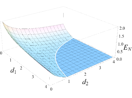
Figure 2: Plot of logarithmic negativity to a two-mode Gaussian state characterized by matrix (49) as the function of excess noises $d_{1}$ and $d_{2}$. The input modes are two-mode squeezed pure states, with squeezing parameter $r=1$.

One can see in Figure 2 that, for any nonzero values of $d_{1}$ and $d_{2}$, the logarithmic negativity is monotonically decreasing. Such effect is the verification process cost. The optimization is reached minimizing the variances of $\hat{p}_{A}$ and $\hat{x}_{B}$, i. e., increasing the squeezing of the probe modes. In addition, the gains $G_{1}$ and $G_{2}$ must be limited, obeying conditions (32), (33), (37), and (38).

VI Discussion

In this paper, a nondestructive scheme for bipartite entanglement verification in the framework of continuous-variable systems was shown. To such task, a suitable choice of QND and beam-splitter interactions between the pair of signal modes and a pair of probe modes is necessary, followed by measurements of the probe modes and feedforward modulations of the signal modes. All of these processes are feasible with current technologies, therefore it can be performed in experimental demonstrations or implemented as a built-in step in a larger communication protocol, in which it is necessary to certify that two signals are entangled, while they are used in another further step. Some studies have already been done with similar purposes in the context of discrete variable systems Barrett05 ; Tang12 ; Liu16 . So this paper fills a gap for continuous-variable systems.

This method is based on a sufficient entanglement condition, therefore some entangled states cannot be detected. However, entangled states that do not satisfy inequality (45) are fragile when subjected to Gaussian attenuation, as already shown in the articles by Barbosa et al. Barbosa10 ; Barbosa11 . So these fragile states would not be interesting for long-distance implementations. Moreover, maximally entangled states or near them are required for many quantum information protocols. Such states are addressed by the scheme.

According to the criteria of QND measurement characterization Imoto89 ; Holland90 ; Blockley90 ; Grangier92 ; Roch92 , we assess the quantum properties of the entanglement verification scheme. One notice that there are many possibilities to calculate the transfer coefficients and the conditional variances, using different quadratures of the bipartite modes. In this paper, we calculate all relevant quantities to certify the QND properties, although we do not present a systematic method for finding them. Therefore a QND multipartite device characterization would be a relevant theoretical development for further research.

The entanglement of the signal modes can be checked by the presented method, but it cannot quantify the entanglement. Such limitation exists because the photocurrents, measured by homodyne detectors, provide information only about the variances of the EPR-like operators, $a_{1}\hat{x}_{1}+a_{2}\hat{x}_{2}$ and $b_{1}\hat{p}_{1}+b_{2}\hat{p}_{2}$. That is insufficient to have a measure of entanglement, e. g., logarithmic negativity, although it is sufficient to detect entanglement. However, new strategies may lead to quantifying the entanglement. We can expect that more complex signal-probe interaction configurations reach these goals. Unlike squeezed vacuum modes, using non-Gaussian modes as probe modes could also lead to more promising results, as already noted in articles concerned with the trade-off between information and disturbance caused by measurements in continuous-variable systems Andersen06 ; Mista06 . All these considerations show many future research possibilities.

We can notice that the entanglement verification is deeply connected with the eavesdropping in quantum cryptography Gisin02 . While an eavesdropper wants to make a necessarily imperfect copy of the signal sent between two communication stations, in the proposed entanglement verification, it looks to observe the correlation between the two signal modes, without necessarily copying and measuring the physical states. The similarity between the two processes is that both are extracting information from the signal, and both are adding unavoidable perturbation, in the case of this paper, adding uncorrelated phase-sensible noise. In both processes, the minimization of the perturbation is the condition to its optimal accomplishment. Further studies may be devoted to the details and explanations of the relationship between the QND verification of multipartite correlations and cloning and eavesdropping.

- (1) M. A. Nielsen and I. L. Chuang, Quantum Computation and Quantum Information (Cambridge University, Cambridge, 2000).
- (2) R. Horodecki, P. Horodecki, M. Horodecki, and K. Horodecki, Rev. Mod. Phys. 81, 865 (2009).
- (3) H. J. Kimble, Nature (London) 453, 1023 (2008).
- (4) J. Yin, J.-G. Ren, H. Lu, Y. Cao, H.-L. Yong, Y.-P. Wu, C. Liu, S.-K. Liao, F. Zhou, Y. Jiang, X.-D. Cai, P. Xu, G.-S. Pan, J.-J. Jia, Y.-M. Huang, H. Yin, J.-Y. Wang, Y.-A. Chen, C.-Z. Peng, and J.-W. Pan, Nature (London) 488, 185 (2012).
- (5) X. S. Ma, T. Herbst, T. Scheidl, D. Wang, S. Kropatschek, W. Naylor, B. Wittmann, A. Mech, J. Kofler, E. Anisimova, V. Makarov, T. Jennewein, R. Ursin, and A. Zeilinger, Nature (London) 489, 269 (2012).
- (6) T. Inagaki, N. Matsuda, O. Tadanaga, M. Asobe, and H. Takesue, Opt. Express 21(20), 23241 (2013).
- (7) T. Scheidl, R. Ursin, A. Fedrizzi, S. Ramelow, X. S. Ma, T. Herbst, R. Prevedel, L. Ratschbacher, J. Kofler, T. Jennewein, and A. Zeilinger, New J. Phys. 11, 085002 (2009).
- (8) S. D. Barrett, P. Kok, K. Nemoto, R. G. Beausoleil, W. J. Munro, and T. P. Spiller, Phys. Rev. A 71, 060302(R) (2005).
- (9) Y.-C. Tang, Y.-S. Li, L. Hao, S.-Y. Hou, and G. L. Long, Phys. Rev. A 85, 022329 (2012).
- (10) Q. Liu, G.-Y. Wang, Q. Ai, M. Zhang, and F.-G. Deng, Sci. Rep. 6, 22016 (2016).
- (11) S. L. Braunstein and P. van Loock, Rev. Mod. Phys. 77, 513 (2005).
- (12) S. L. Braunstein and H. J. Kimble, Phys. Rev. Lett. 80, 869 (1998).
- (13) A. Furusawa, J. L. Sørensen, S. L. Braunstein, C. A. Fuchs, H. J. Kimble, E. S. Polzik, Science 282, 706 (1998).
- (14) W. P. Bowen, N. Treps, B. C. Buchler, R. Schnabel, T. C. Ralph, H.-A. Bachor, T. Symul, P.-K. Lam, Phys. Rev. A 67, 032302 (2003).
- (15) T. C. Zhang, K. W. Goh, C. W. Chou, P. Lodahl, H. J. Kimble, Phys. Rev. A 67, 033802 (2003).
- (16) V. Bužek and M. Hillery, Phys. Rev. A 54, 1844 (1996).
- (17) L. K. Grover, arXiv:quant-ph/9704012; J. I. Cirac, A. K. Ekert, S. F. Huelga, and C. Macchiavello, Phys. Rev. A 59, 4249 (1999).
- (18) U. L. Andersen, V. Josse, and G. Leuchs, Phys. Rev. Lett. 94, 240503 (2005).
- (19) M. Murao, D. Jonathan, M. B. Plenio, and V. Vedral, Phys. Rev. A 59, 156 (1999).
- (20) P. van Loock and S. L. Braunstein, Phys. Rev. Lett. 87, 247901 (2001).
- (21) S. Koike, H. Takahashi, H. Yonezawa, N. Takei, S. L. Braunstein, T. Aoki, and Akira Furusawa, Phys. Rev. Lett. 96, 060504 (2006).
- (22) V. B. Braginsky, Yu. I. Vorontsov, and K. S. Thorne, Science 209, 547 (1980).
- (23) V. B. Braginsky and F. Ya. Khalili, Rev. Mod. Phys. 68, 1 (1996).
- (24) P. Grangier, J. A. Levenson, and J.-P. Poizat, Nature (London) 396, 537 (1998).
- (25) H. M. Wiseman and G. J. Milburn, Quantum Measurement and Control (Cambridge University, New York, 2010).
- (26) G. J. Milburn and D. F. Walls, Phys. Rev. A 28, 2065 (1983).
- (27) N. Imoto, H. A. Haus, and Y. Yamamoto, Phys. Rev. A 32, 2287 (1985).
- (28) M. D. Levenson, R. M. Shelby, M. Reid, and D. F. Walls, Phys. Rev. Lett. 57, 2473 (1986).
- (29) B. Yurke, J. Opt. Soc. Am. B 2, 732 (1985).
- (30) A. La Porta, R. E. Slusher, and B. Yurke, Phys. Rev. Lett. 62, 28 (1989).
- (31) B. C. Buchler, P. K. Lam, and T. C. Ralph, Phys. Rev. A 60, 4943 (1999).
- (32) U. L. Andersen, B. C. Buchler, H.-A. Bachor, and P. K. Lam, J. Opt. B: Quantum Semiclass. Opt. 4, S229 (2002).
- (33) R. Filip, P. Marek, and U. L. Andersen, Phys. Rev. A 71, 042308 (2005).
- (34) J. Yoshikawa, Y. Miwa, A. Huck, U. L. Andersen, P. van Loock, and A. Furusawa, Phys. Rev Lett. 101, 250501 (2008).
- (35) B. C. Buchler, P. K. Lam, H.-A. Bachor, U. L. Andersen, and T. C. Ralph, Phys. Rev. A 65, 011803R (2001).
- (36) J. Yoshikawa, T. Hayashi, T. Akiyama, N. Takei, A. Huck, U. L. Andersen, and A. Furusawa, Phys. Rev. A 76, 060301(R) (2007).
- (37) K. Miyata, H. Ogawa, P. Marek, R. Filip, H. Yonezawa, J. Yoshikawa, and A. Furusawa, Phys. Rev. A 90, 060302(R) (2014).
- (38) R. Ukai, N. Iwata, Y. Shimokawa, S. C. Armstrong, A. Politi, J. Yoshikawa, P. van Loock, and A. Furusawa, Phys. Rev. Lett. 106, 240504 (2011).
- (39) S. Yokoyama, R. Ukai, S. C. Armstrong, J. Yoshikawa, P. van Loock, and A. Furusawa, Phys. Rev. A 92, 032304 (2015).
- (40) P. Marek, R. Filip, and A. Furusawa, Phys. Rev. A 84, 053802 (2011).
- (41) P. Marek and R. Filip, Phys. Rev. A 81, 042325 (2010).
- (42) S. Yokoyama, R. Ukai, J. Yoshikawa, P. Marek, R. Filip, and A. Furusawa, Phys. Rev. A 90, 012311 (2014).
- (43) T. C. Ralph, Phys. Rev. A 56, 4187 (1997).
- (44) P. K. Lam, T. C. Ralph, E. H. Huntington, and H.-A. Bachor, Phys. Rev. Lett. 79, 1471 (1997).
- (45) E. H. Huntington, P. K. Lam, T. C. Ralph, D. E. McClelland, and H.-A. Bachor, Opt. Lett. 23, 540 (1998).
- (46) R. Simon, Phys. Rev. Lett. 84, 2726 (2000).
- (47) L.-M. Duan, G. Giedke, J. I. Cirac, and P. Zoller, Phys. Rev. Lett. 84, 2722 (2000).
- (48) N. Imoto and S. Saito, Phys. Rev. A 39, 675 (1989).
- (49) M. J. Holland, M. J. Collett, D. F. Walls, and M. D. Levenson, Phys. Rev. A 42, 2995 (1990).
- (50) C. A. Blockley and D. F. Walls, Opt. Commun. 79, 241 (1990).
- (51) P. Grangier, J.-M. Courty, and S. Reynaud, Opt. Commun. 89, 99 (1992).
- (52) J. F. Roch, G. Roger, P. Grangier, J.-M. Courty and S. Reynaud, Appl. Phys. B 55, 291 (1992).
- (53) R. Simon in Quantum Information with Continuous Variables, edited by S. L. Braunstein and A. K. Pati (Kluwer Academic, Dordrecht, 2001), p. 155.
- (54) V. Giovannetti, S. Mancini, D. Vitali, and P. Tombesi, Phys. Rev. A 67, 022320 (2003).
- (55) C. Weedbrook, S. Pirandola, R. García-Patrón, N. J. Cerf, T. C. Ralph, J. H. Shapiro, and S. Lloyd, Rev. Mod. Phys. 84, 621 (2012).
- (56) G. Vidal and R. F. Werner, Phys. Rev. A 65, 032314 (2002).
- (57) G. Adesso, A. Serafini, and F. Illuminati, Phys. Rev. A 70, 022318 (2004).
- (58) M. B. Plenio, Phys. Rev. Lett. 95, 090503 (2005).
- (59) F. A. S. Barbosa, A. S. Coelho, A. J. de Faria, K. N. Cassemiro, A. S. Villar, P. Nussenzveig, and M. Martinelli, Nature Photonics 4, 858 (2010).
- (60) F. A. S. Barbosa, A. J. de Faria, A. S. Coelho, K. N. Cassemiro, A. S. Villar, P. Nussenzveig, and M. Martinelli, Phys. Rev. A 84, 052330 (2011).
- (61) U. L. Andersen, M. Sabuncu, R. Filip, and G. Leuchs, Phys. Rev. Lett. 96, 020409 (2006).
- (62) L. Mišta, Jr., Phys. Rev. A 73, 032335 (2006).
- (63) N. Gisin, G. Ribordy, W. Tittel, and H. Zbinden, Rev. Mod. Phys. 74, 145 (2002).