Heralded entanglement of two distant quantum dot spins via optical interference

Abstract

We present a proposal for heralded entanglement between two quantum dots via Hong–Ou–Mandel effect. Each of the quantum dots, drived off-resonance by two lasers, can be entangled with the coherent cavity mode. The output photons from the two coherent cavity modes interfering by a beamsplitter, we could entangle the two QDs with nearly unit success probability. Our scheme requires neither direct coupling between qubits nor the detection of single photons. Moreover the quantum dots do not need to have the same frequencies and coupling constants.

I Introduction

Quantum entanglement is treated as a crucial resource in many quantum information tasks, such as quantum teleportation bennett , quantum dense coding bennett2 , quantum cryptography and quantum computation Ekert . Most of the tasks require generating entanglement among distant quantum nodes. However, it is not easy to generate entanglement between distant nodes, as interaction between qubit is generally local. In order to solve the problem, many schemes of creating entanglement between spatially separated nodes have been proposed cirac ; Enk ; feng ; yao1 ; yao2 ; yin ; libo ; Schwager1 ; Schwager2 and some experimentally demonstrated duan ; duan2 ; Sangouard ; Bernien ; Usmani . These schemes are either probabilistic or have yet to be demonstrated experimentally.

Recently, spin qubits in semiconductor quantum dots (QDs) attract much interest because of their potential for a compact and scalable quantum information architecture, and relatively long coherence time loss . It has been demonstrated that double quantum dots can be entangled by directly coupling D.kim . However, the method cannot be used to entangle the distant quantum dots. It is found that semiconductor QDs can be strongly coupled to photonic crystal cavity systems Hennessy ; Englund . However, due to the dot size variation, semiconductor QDs usually have different radiative properties, which make it difficult to generate entanglement by indistinguishable emitting photons, as those have been done in atomic systems. There are two approaches to overcome the problem: (i) tuning the QDs into resonance by using externally applied strain Flagg ; Patel , or controlling the Overhauser field x.xu2 ; gong or (ii) making a detuning between quantum dots and the same frequency output cavity modes Busch ; Sridharan ; waks , or using quantum frequency conversion Ates ; Zaske . There has, to our best knowledge, been no reported experimental realization of entanglement between two distant QDs. In Ref. Busch QDs in low Q cavities are coupled to a common high-Q cavity mode. There are no reliable device structures like this yet. In Ref. Sridharan ; waks weak coherent fields being reflected from the Cavity-QDs system have low efficiency or success possibility. Recently, schemes for robust multiphoton entanglement creation using coherent (or Gaussian) state light were put forward chan ; cohen . The rate is much larger than the single-photon entanglement creation schemes duan ; duan2 ; Sangouard ; Usmani .

In this paper, we describe a protocol for generating entanglement between two quantum dots via Hong–Ou–Mandel effect hom . The QDs are strongly driven by $V$ polarized laser fields, generating $H$ polarized coherent cavity modes which separately entangle with the two QDs. The output photons from the two coherent cavity modes interfering by a beamsplitter, we could entangle the two QDs with nearly unit efficiency and fidelity. The scheme does not need the quantum dots to have the same radiation frequency. Compared with the entanglement distributing schemes reported previously duan ; duan2 ; Sangouard , our scheme combines both the advantages that appear in direct coupling method (high efficiency) and single photon interference method (high fidelity) Spiller . We believe that our protocol is a promising route to a scalable quantum computation in solid system.

II Entanglement of two quantum dots

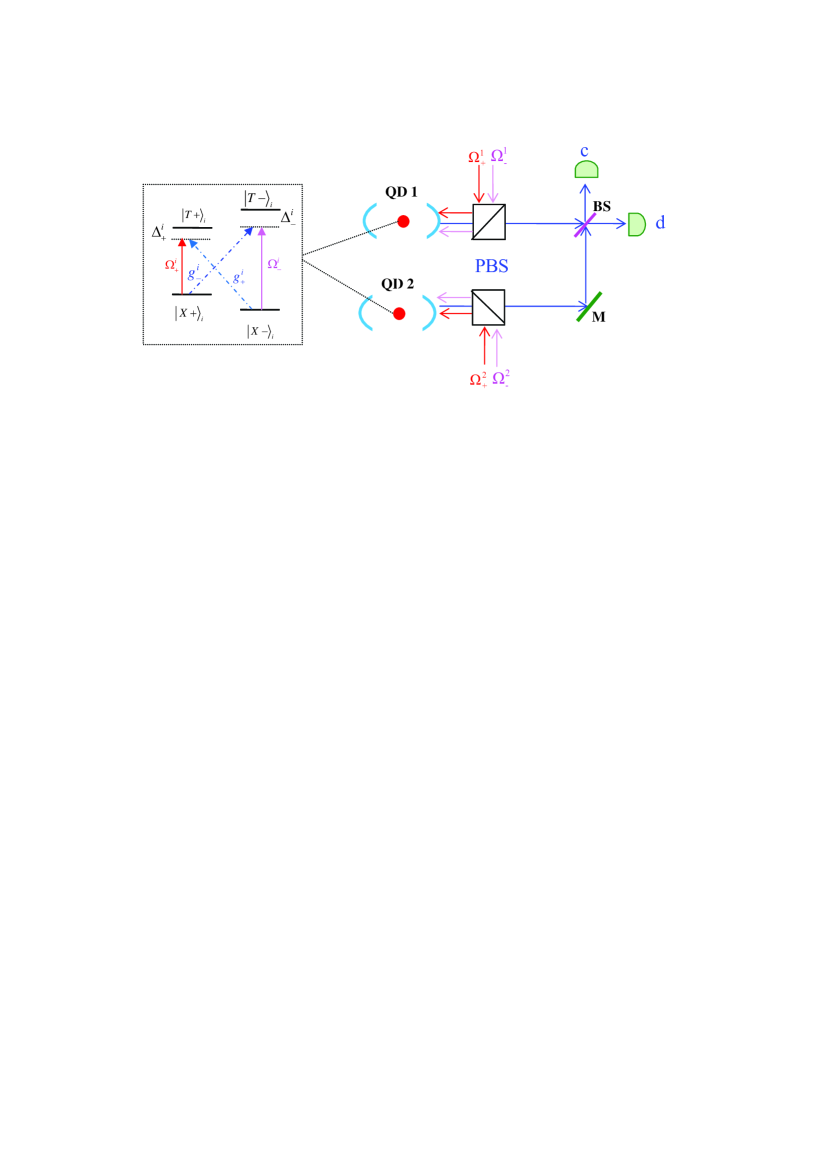
Figure 1: [Color online] Two quantum dots are embedded in two cavities with the same frequency. The $\left|X+\right\rangle_{i}\rightarrow\left|T+\right\rangle_{i}$ transition of dot $i$ is driven by a $V$ polarized laser pulse with Rabbi frequency $\Omega_{+}^{i}$ and detuning $\Delta_{+}^{i}$. Another $V$ polarized laser pulse drives the transition $\left|X-\right\rangle_{i}\rightarrow\left|T-\right\rangle_{i}$ with Rabbi frequency $\Omega_{-}^{i}$ and detuning $\Delta_{-}^{i}$. The $\left|X+\right\rangle_{i}\rightarrow\left|T-\right\rangle_{i}$ and $\left|X-\right\rangle_{i}\rightarrow\left|T+\right\rangle_{i}$ transitions couple the $H$ polarized cavity mode $a_{i}$ with detuning $\Delta_{-}^{i}$ and $\Delta_{+}^{i}$ and coupling strength $g_{-}^{i}$ and $g_{+}^{i}$. After passing though Polarized Beam Splitters ($PBS$s), the output modes are mixed with a $50:50$ Beam Splitter ($BS$) and measured by photodetectors $c$ and $d$.

Suppose that two quantum dots are seperately coupled to two cavities with same cavity mode frequency. The internal level configuration of each quantum dot is shown in the left part of Fig. 1 Busch ; x.xu ; x.xu2 . The $\left|X+\right\rangle_{i}\rightarrow\left|T+\right\rangle_{i}$ transition of dot $i$ is driven by a $V$ polarized laser pulse with Rabbi frequency $\Omega_{+}^{i}$ and detuning $\Delta_{+}^{i}$. Another $V$ polarized laser pulse drives the transition $\left|X-\right\rangle_{i}\rightarrow\left|T-\right\rangle_{i}$ with Rabbi frequency $\Omega_{-}^{i}$ and detuning $\Delta_{-}^{i}$. The $\left|X+\right\rangle_{i}\rightarrow\left|T-\right\rangle_{i}$ and $\left|X-\right\rangle_{i}\rightarrow\left|T+\right\rangle_{i}$ transitions couple the $H$ polarized cavity mode $a_{i}$ with detuning $\Delta_{-}^{i}$ and $\Delta_{+}^{i}$ and coupling strength $g_{-}^{i}$ and $g_{+}^{i}$. (By choosing the detunings, the two quantum dots can coupled the same frequency cavities). Introducing the rotating wave approximation and choosing the appropriate interaction picture, the Hamiltonian is ($\hbar=1$)

$$H =\sum_{i=1,2}[\Omega_{+}^{i}e^{-i\Delta_{+}^{i}}\left|X+\right\rangle_{i}\left\langle T+\right|+\Omega_{-}^{i}e^{-i\Delta_{-}^{i}}\left|X-\right\rangle_{i}\left\langle T-\right|$$

$$+g_{+}^{i}e^{-i\Delta_{+}^{i}}\left|X-\right\rangle_{i}\left\langle T+\right|a_{i}^{+}+g_{-}^{i}e^{-i\Delta_{-}^{i}}\left|X+\right\rangle_{i}\left\langle T-\right|a_{i}^{+}+H.c.]\text{,}$$ (1)

under the condition

$$\Omega_{+}^{i}\text{, }\Omega_{-}^{i}\text{, }g_{-}^{i}\text{, }g_{+}^{i}\ll\Delta_{-}^{i}\text{, }\Delta_{+}^{i}\text{,}$$ (2)

and choose

$$\frac{\Omega_{+}^{i}g_{+}^{i}}{\Delta_{+}^{i}}=\frac{\Omega_{-}^{i}g_{-}^{i}}{\Delta_{-}^{i}}=\lambda_{i}\text{,}$$ (3)

the Hamiltonian (1) simplifies to

$$H_{\text{eff}}=\sum_{i=1,2}[\lambda_{i}(\left|X-\right\rangle_{i}\left\langle X+\right|+\left|X+\right\rangle_{i}\left\langle X-\right|)a_{i}^{+}+H.c.]\\ =\sum_{i=1,2}\lambda_{i}\sigma_{y}^{i}\left(a_{i}^{+}+a_{i}\right)$$

here $\sigma_{y}^{i}=\left|X-\right\rangle_{i}\left\langle X+\right|+\left|X+\right\rangle_{i}\left\langle X-\right|$, so$\ \left|y+\right\rangle_{i}=\frac{1}{\sqrt{2}}\left(\left|X-\right\rangle_{i}+\left|X+\right\rangle_{i}\right)$ and $\left|y-\right\rangle_{i}=\frac{1}{\sqrt{2}}\left(\left|X-\right\rangle_{i}-\left|X+\right\rangle_{i}\right)$.

$$e^{-iH_{\text{eff}}t}\left|y+\right\rangle_{i}\left|0\right\rangle_{c}^{i}=\left|y+\right\rangle_{i}\left|-\alpha_{i}\right\rangle_{c}^{i}\text{,}$$

$$e^{-iH_{\text{eff}}^{\prime}t}\left|y-\right\rangle_{i}\left|0\right\rangle_{c}^{i}=\left|y-\right\rangle_{i}\left|\alpha_{i}\right\rangle_{c}^{i}\text{,}$$

here $\alpha_{i}=-i\lambda_{i}t$, and $\left|m\right\rangle_{c}^{i}$ represents the state of the cavity mode $a_{i}$. If our initial state of the dot–cavity combined system is $\sum_{i=1,2}\left|X-\right\rangle_{i}\left|0\right\rangle_{c}^{i}$, under the Hamiltonian $H_{\text{eff}}$, the state of the system evolve to

$$\left|\psi\left(t\right)\right\rangle=e^{-iH_{\text{eff}}t}{\displaystyle\prod\limits_{i=1,2}}\left|X-\right\rangle_{i}\left|0\right\rangle_{c}^{i}\\ =\frac{1}{2}e^{-iH_{\text{eff}}t}{\displaystyle\prod\limits_{i=1,2}}\left(\left|y+\right\rangle_{i}+\left|y-\right\rangle_{i}\right)\left|0\right\rangle_{c}^{i}\\ =\frac{1}{2}{\displaystyle\prod\limits_{i=1,2}}\left(\left|y+\right\rangle_{i}\left|\alpha_{i}\right\rangle_{c}^{i}+\left|y-\right\rangle_{i}\left|-\alpha_{i}\right\rangle_{c}^{i}\right)\text{.}$$

The mode $\widehat{a}_{1}^{out}$ ( $\widehat{a}_{2}^{out}$ ) output from the cavity $1$ ($2$) reaches the beamsplitter ($BS$). The $BS$ then applies the transformations

$$\widehat{a}_{1}^{out} \rightarrow\frac{\widehat{c}+\widehat{d}}{\sqrt{2}}\text{,}$$ (4)

$$\widehat{a}_{2}^{out} \rightarrow\frac{\widehat{c}-\widehat{d}}{\sqrt{2}}\text{,}$$ (5)

where $\widehat{c}\$and $\widehat{d}$ are the bosonic modes monitored by detector $c$ and detector $d$ respectively. In the case of $\alpha_{1}=\alpha_{2}=\alpha$, the state of the system becomes

$$\left|\psi\left(t\right)\right\rangle_{f}=\frac{1}{2}(\left|y+\right\rangle_{1}\left|y+\right\rangle_{2}\left|\sqrt{2}\alpha\right\rangle_{c}\left|\text{vac}\right\rangle_{d}+\left|y+\right\rangle_{1}\left|y-\right\rangle_{2}\left|\text{vac}\right\rangle_{c}\left|-\sqrt{2}\alpha\right\rangle_{d}$$

$$\text{ \ \ \ \ }+\left|y-\right\rangle_{1}\left|y+\right\rangle_{2}\left|\text{vac}\right\rangle_{c}\left|\sqrt{2}\alpha\right\rangle_{d}+\left|y-\right\rangle_{1}\left|y-\right\rangle_{2}\left|-\sqrt{2}\alpha\right\rangle_{c}\left|\text{vac}\right\rangle_{d})\text{,}$$ (6)

where The state $\left|\text{vac}\right\rangle$ represents the vacuum state of field mode. Conditioned on photons detection event at detector $c$, the state of the QDs collapses onto

$$\left|\phi\right\rangle_{1}=\frac{1}{\sqrt{2}}(\left|y+\right\rangle_{1}\left|y+\right\rangle_{2}+\left|y-\right\rangle_{1}\left|y-\right\rangle_{2})\text{,}$$ (7)

photons detection event at detector $d$, the state of the QDs collapses onto

$$\left|\phi\right\rangle_{2}=\frac{1}{\sqrt{2}}(\left|y+\right\rangle_{1}\left|y-\right\rangle_{2}+\left|y-\right\rangle_{1}\left|y+\right\rangle_{2})\text{,}$$ (8)

It should be noted that, so long as detector is triggered, a perfect entangled state can be generated heraldedly even when the QDs have different resonant frequencies.

III Simulations with the Lindblad master equation

The system consists of two cavity modes $\hat{a}_{1},\hat{a}_{2}$ and two quantum dots. In the absence of any photon detection, the system evolution obeys the Lindblad master equation

$$\dot{\rho}(t) =i[H,\rho(t)]-\sum_{i=1,2}[\frac{\kappa_{i}}{2}\left(a_{i}^{+}a_{i}\rho(t)-2a_{i}^{+}\rho(t)a_{i}+\rho(t)a_{i}^{+}a_{i}\right)$$

$$-\frac{\Gamma_{i}}{2}\left(\left|X+\right\rangle_{i}\left\langle X+\right|\rho(t)-2\left|X-\right\rangle_{i}\left\langle X+\right|\rho(t)\left|X+\right\rangle_{i}\left\langle X-\right|+\rho(t)\left|X+\right\rangle_{i}\left\langle X+\right|\right)]\text{,}$$ (9)

where $\Gamma_{i}$ denotes the relaxation of the two QDs and $\kappa_{i}$ the damping of the two cavities. The steady state $\hat{\rho}_{\mathrm{ss}}(t)$ of the system can be obtained by solving the Lindblad master equation.

Now each cavity is coupled to a transmission line. The output of these two transmission lines are mixed by a $50:50$ beam splitter and each port of the beamsplitter is monitored by photon counter. The output electric field $\hat{b}_{j,\mathrm{out}}(t)$ of the $j$th $(j=1,2)$ transmission line carries information about the cavity:

$$\hat{b}_{1,\mathrm{out}}(t) =-i\sqrt{\kappa_{1}}\hat{a}_{1}(t)\text{,}$$

$$\hat{b}_{2,\mathrm{out}}(t) =-i\sqrt{\kappa_{2}}\hat{a}_{2}(t)\text{,}$$ (10)

where the vacuum fluctuation part $\hat{b}_{1,\mathrm{in}}(t)$ and $\hat{b}_{2,\mathrm{in}}(t)$ have been neglected, since they have no effect on the photon counter. The output field of the beam splitter is

$$\hat{c}(t) =[\hat{b}_{1,\mathrm{out}}(t)+i\hat{b}_{2,\mathrm{out}}(t)]/\sqrt{2}$$

$$=-i[\sqrt{\kappa_{1}}\hat{a}_{1}(t)+\sqrt{\kappa_{2}}\hat{a}_{2}(t)]/\sqrt{2}\text{,}$$ (11)

$$\hat{d}(t) =[\hat{b}_{1,\mathrm{out}}(t)-i\hat{b}_{2,\mathrm{out}}(t)]/\sqrt{2}$$

$$=-i[\sqrt{\kappa_{1}}\hat{a}_{1}(t)-\sqrt{\kappa_{2}}\hat{a}_{2}(t)]/\sqrt{2}\text{.}$$ (12)

During $[t,t+dt]$ ($dt\rightarrow 0$ is an infinitesimal interval), photon detection $c$ occurs with probability

$$p\left(dt\right)=dt\operatorname*{Tr}\hat{c}\hat{\rho}_{\mathrm{ss}}(t)\hat{c}^{\dagger}\text{,}$$ (13)

after which the system collapses to the state (un-normalized) $\tilde{\rho}^{(1)}(t+dt)=\hat{c}\hat{\rho}_{\mathrm{ss}}(t)\hat{c}^{\dagger}dt$. Fig. 2 plots of the average detecting photon number $N$ vs $\lambda t$ for different values of $\kappa/\lambda$, here we choose $\lambda_{1}=\lambda_{2}=\lambda$, $\kappa_{1}=\kappa_{2}=\kappa$, $\Gamma_{1}=\Gamma_{2}=\Gamma$, and $\Gamma=0.05\lambda$. In the case of the detector $c$ (or $d$) is triggered, Fig. 2 plots the fidelity of the entanglemnt state $F$ vs $\lambda t$ for different values of $\kappa/\lambda$, here we choose $\kappa=\lambda$.

We use parameters appropriate for self-assembled InAs QDs, $\delta=\Delta_{-}-\Delta_{+}=(\omega_{T-}-\omega_{T+})+(\omega_{X-}-\omega_{X+})=46$ $\mu$eV x.xu ; Economou , $g_{+}=g_{-}=90$ $\mu$eV Hennessy , $\Delta_{-}=460$ $\mu$eV, $\Delta_{+}=414$ $\mu$eV, $\Omega_{+}=41.4$ $\mu$eV, and $\Omega_{-}=46$ $\mu$eV. With these parameters, the conditions given by equations (2) and (3) are fulfilled and value $\lambda=2.2$ $G$Hz is obtained. In realistic experiments, the spontaneous decay rate of the trion state $\left|T\pm\right\rangle$ is about $\Gamma_{T}=2\pi\times 130$ MHz x.xu3 . Fig. 4 plots the population of the trion state $\left|T\pm\right\rangle$ by using the above parameters. Due to large detuning, the effective decay rate could be estimated as $\Gamma_{T}\Omega g/\Delta^{2}\approx 2\pi\times 2.6$ MHz Pellizzari ; W.L.Yang , which is much smaller than $\lambda$. This implies that the influence from the spontaneous decay in our scheme. The main source of error is the depahsing of elecron spin. The typical dephasing rate of the InAs QD electron spin has been measured to be about $\Gamma=\left(10ns\right)^{-1}\approx 0.05\lambda$ Bracker , the fidelity of the entanglemnt state is larger than $0.95$ as shown in Fig. 3. From the Fig. 3. and 4 we can neglect the influence the trion state $\left|T\pm\right\rangle$.

IV Conclusion

In conclusion, we have generated deterministic entanglement between two distant quantum dots using classical interference; that is, there is no inherent probabilistic nature to our quantum entangling source. The method is robust to the difference of the two quantum dots and cavities. Our scheme does not need to control coupling between qubits nor to detection of single photons. Using this larger arrays of quantum dot qubits could be linked together for scale-up to a quantum computer Stoneham .

Acknowledgments: We thanks Prof. Lu Jeu Sham and Dr. Jianqi Zhang for helpful discussions. This research is supported the National Natural Science Foundation of China (Grant No.11304174), Natural Science Foundation of Shandong Province (Grant No. ZR2013AQ010), and the research starting foundation of Qingdao Technological University.

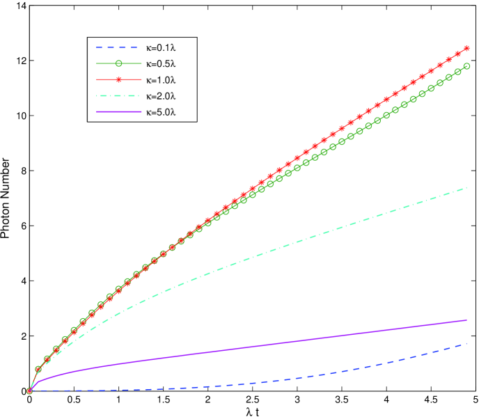
Figure 2: [Color online] The average leaking photon number $N$ vs $\lambda t$ for different values of $\kappa/\lambda$ (From bottom to top, $\kappa/\lambda=0.1$, $0.2$, $0.5$, $1.0$).

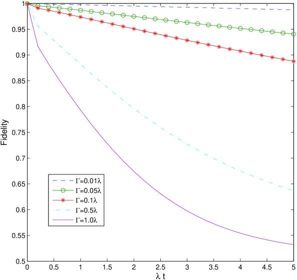
Figure 3: The fidelity of the entanglemnt state $F$ vs $\lambda t$ for different values of $\kappa/\lambda$ (From top to bottom, $\Gamma/\lambda=0.01$, $0.05$, $0.1$, $0.5$, $1.0$), here we choose $\kappa=\lambda$.

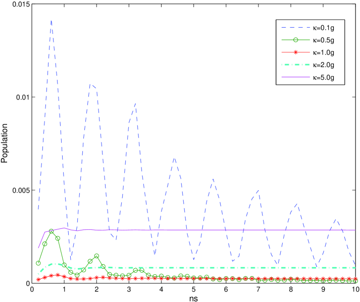
Figure 4: The population of the trion state $\left|T\pm\right\rangle$, here we choose $\delta=46$ $\mu$eV , $g_{+}=g_{-}=90$ $\mu$eV , $\Delta_{-}=460$ $\mu$eV, $\Delta_{+}=414$ $\mu$eV, $\Omega_{+}=41.4$ $\mu$eV, and $\Omega_{-}=46$ $\mu$eV, $\Gamma_{T}=2\pi\times 130$ MHz.

References

• (1) C. H. Bennett, G. Brassard, C. Crepeau, R. Jozsa, A. Peres, W. K. Wootters, Phys. Rev. Lett. 70, 1895 (1993).
• (2) C. H. Bennett, S. J. Wiesner, Phys. Rev. Lett. 69, 2881 (1992).
• (3) A.K. Ekert Phys. Rev. Lett. 67, 661 (1991).
• (4) J. I. Cirac, P. Zoller, H. J. Kimble, and H. Mabuchi, Phys. Rev. Lett. 78, 3221 (1997).
• (5) S. J. van Enk, J. Cirac, and P. Zoller, Phys. Rev. Lett. 78, 4293 (1997).
• (6) X. L. Feng, Z. M. Zhang, X. D. Li, S. Q. Gong, and Z. Z. Xu, Phys. Rev. Lett. 90, 217902 (2003).
• (7) W. Yao, R. B. Liu, and L. J. Sham, Phys. Rev. Lett. 95, 030504 (2005).
• (8) W. Yao, R. B. Liu, and L. J. Sham, J. Opt. B: Quantum Semiclassical Opt. 7, 318 (2005).
• (9) Z. Q. Yin and F. L. Li, Phys. Rev. A 75, 012324 (2007).
• (10) L. B. Chen, M. Y. Ye, G. W. Lin, Q. H. Du, and X. M. Lin, Rev. A 76, 062304 (2007).
• (11) H. Schwager, J. I. Cirac, and G. Giedke, Phys. Rev. B 81, 045309 (2010).
• (12) H. Schwager, J. I. Cirac, and G. Giedke, New J. Phys. 12, 043026 (2010).
• (13) L. M. Duan, M. D. Lukin, J. I. Cirac, and P. Zoller, Nature (London) 414, 413 (2001).
• (14) L. M. Duan and C. Monroe, Rev. Mod. Phys. 82, 1209 (2010).
• (15) N. Sangouard, C. Simon, H. de Riedmatten, and N. Gisin, Rev. Mod. Phys. 83, 33 (2011).
• (16) D. Kim, S. Carter, A. Greilich, A. Bracker, and D. Gammon, Nature (London) 497, 86 (2013).
• (17) I. Usmani, C. Clausen, F. Bussières, N. Sangouard, M. Afzelius and N. Gisin, Nature Photon. 6, 234 (2012).
• (18) D. Loss and D. P. DiVincenzo, Phys. Rev. A 57, 120 (1998).
• (19) D. Kim, S. Carter, A. Greilich, A. Bracker, and D. Gammon, Nature Phys. 7, 223 (2011).
• (20) K. Hennessy, A. Badolato, M. Winger, D. Gerace, M. Atatüre, S. Gulde, S. Fält, E. L. Hu, and A. Imamoğlu, Nature (London) 445, 896 (2007).
• (21) D. Englund, D. Fattal, E. Waks, G. Solomon, B. Zhang, T. Nakaoka, Y. Arakawa, Y. Yamamoto, and J. Vučković, Phys. Rev. Lett. 95, 013904 (2005).
• (22) E. B. Flagg, A. Muller, S. V. Polyakov, A. Ling, A. Migdall, and G. S. Solomon, Phys. Rev. Lett. 104, 137401 (2010).
• (23) R. B. Patel, A. J. Bennett, I. Farrer, C. A. Nicoll, D. A. Ritchie, and A. J. Shields, Nat. Photonics 4, 632 (2010).
• (24) X. Xu, W. Yao, B. Sun, D. G. Steel, A. S. Bracker, D. Gammon, and L. J. Sham, Nature (London) 459, 1105 (2009).
• (25) Z. X. Gong, Z. Q. Yin, and L. M. Duan, New J. Phys. 13, 033036 (2011).
• (26) J. Busch, E. S. Kyoseva, M. Trupke, and A. Beige, Phys. Rev. A 78, 040301(R) (2008).
• (27) D. Sridharan and E. Waks, Phys. Rev. A 78, 052321 (2008).
• (28) E. Waks and C. Monroe, Phys. Rev. A 80, 062330 (2009).
• (29) S. Ates, I. Agha, A. Gulinatti, I. Rech, M. T. Rakher, A. Badolato, and K. Srinivasan, Phys. Rev. Lett. 109, 147405 (2012).
• (30) S. Zaske, A. Lenhard, C. A. Kessler, J. Kettler, C. Hepp, C. Arend, R. Albrecht,W.-M. Schulz, M. Jetter, P. Michler, and C. Becher, Phys. Rev. Lett. 109, 147404 (2012)
• (31) C.-K. Chan and L. J. Sham, Phys. Rev. Lett. 110, 070501 (2013).
• (32) Guy Z. Cohen and L. J. Sham, Phys. Rev. B 88 , 245306 (2013).
• (33) C. K. Hong, Z. Y. Ou, and L. Mandel, Phys. Rev. Lett. 59, 2044 (1987).
• (34) T. P. Spiller, K. Nemoto, S. L. Braunstein, W. J. Munro, P. van Loock, and G. J. Milburn, New J. Phys. 8, 30 (2006).
• (35) X. Xu, Y. Wu, B. Sun, Q. Huang, J. Cheng, D. G. Steel, A. S. Bracker, D. Gammon, C. Emary, and L. J. Sham, Phys. Rev. Lett. 99, 097401 (2007).
• (36) S. E. Economou and T. L. Reinecke, Phys. Rev. Lett. 99, 217401 (2007).
• (37) A. S. Bracker et al., Phys. Rev. Lett. 94, 047402 2005 .
• (38) X. Xu, B. Sun, P. R. Berman, D. G. Steel, A. S. Bracker, D. Gammon, and L. J. Sham, Science 317, 929 (2007).
• (39) T. Pellizzari, Phys. Rev. Lett. 79, 5242 (1997).
• (40) W. L. Yang, Z. Q. Yin, Z. Y. Xu, M. Feng, and J. F. Du, Appl. Phys. Lett. 96, 241113 (2010).
• (41) A. M. Stoneham, Phys. 2, 34 (2009).
Refer to caption