Hyperbolization of cusps with convex boundary

Abstract.

We prove that for every metric on the torus with curvature bounded from below by $-1$ in the sense of Alexandrov there exists a hyperbolic cusp with convex boundary such that the induced metric on the boundary is the given metric. The proof is by polyhedral approximation.

This was the last open case of a general theorem: every metric with curvature bounded from below on a compact surface is isometric to a convex surface in a $3$-dimensional space form.

1. Introduction

1.1. Statement of the results

Let $T$ denote the $2$-dimensional torus. A hyperbolic cusp $\mathrm{C}$ with convex boundary is a complete hyperbolic manifold of finite volume, homeomorphic to $T\times[0,+\infty[$, and such that the boundary $\partial\mathrm{C}=T\times\{0\}$ is geodesically convex. By the Buyalo convex hypersurface theorem [AKP08], the induced inner metric on $\partial\mathrm{C}$ has curvature bounded from below by $-1$ in the sense of Alexandrov — in short, the metric is CBB($-1$), see Section 2.1. In the present paper, we prove that all the CBB($-1$) metrics on the torus are obtained in this way.

Theorem 1.1.

Let $m$ be a CBB($-1$) metric on the torus. Then there exists a hyperbolic cusp $\mathrm{C}$ with convex boundary such that the induced metric on $\partial\mathrm{C}$ is isometric to $m$.

Throughout the paper, by induced metric we mean an intrinsic metric. Examples of CBB($-1$) metrics on the torus are distances defined by Riemannian metrics of curvature $\geq-1$. Using classical regularity results by Pogorelov (see below), Theorem 1.1 implies the following.

Theorem 1.2.

Let $g$ be a smooth Riemannian metric of curvature $>-1$ on the torus. Then there exists a hyperbolic cusp $\mathrm{C}$ with smooth strictly convex boundary such that the induced Riemannian metric on $\partial\mathrm{C}$ is isometric to $g$.

Another examples of CBB($-1$) metrics on the torus are hyperbolic metrics with conical singularities of positive curvatures. Recall that the (singular) curvature at a cone singularity is $2\pi$ minus the total angle around the singularity. The proof of Theorem 1.1 will be done by polyhedral approximation, using the following result.

Theorem 1.3 ([FI09]).

Let $m$ be a hyperbolic metric with conical singularities of positive curvature on the torus. Then there exists a hyperbolic cusp $\mathrm{C}$ with convex polyhedral boundary such that the induced inner metric on $\partial\mathrm{C}$ is isometric to $m$.

Actually it is proved in [FI09] that the cusp $\mathrm{C}$ in the statement of Theorem 1.3 is unique. One can hope a uniqueness result in Theorem 1.1 (that would also imply uniqueness in Theorem 1.2). This should be the subject of a forthcoming paper.

The above statements were the last steps in order to get the following general statement.

Theorem 1.4.

Let $m$ be a CBB($k$) metric on a compact surface. Then $m$ is isometric to a convex surface $S$ in a Riemannian space of constant curvature $k$. Moreover

• if $m$ is a metric of curvature $k$ with conical singularities of positive curvature, then $S$ is polyhedral,

• if $m$ comes from a smooth Riemannian metric with curvature $>k$, then $S$ is smooth and strictly convex.

In Section 1.2 we will recall all the results leading to Theorem 1.4. The proof of Theorem 1.1 is based on a general result of polyhedral approximation that is recalled in Section 2.1 (Theorem 2.2). Going to the universal cover, boundaries of convex hyperbolic cusps are seen as convex surfaces of the hyperbolic space invariant under the action of a group of isometries acting cocompactly on a horosphere. Such surfaces are graphs of horoconvex functions defined on the horosphere. They are introduced in Section 2.2. They can be written in terms of convex functions on the plane, hence they will inherit strong properties from convex functions.

Then we prove Theorem 1.1 in Section 3. Theorem 1.3 and Theorem 2.2 give a sequence of polyhedral surfaces in ${\mathbb{H}}^{3}$. One shows that this sequence converges to a convex surface, invariant under the action of a group $\Gamma$. The main point is to check that the induced metric on the quotient of the surface by $\Gamma$ is isometric to the metric $m$ (Section 3.4).

1.2. Hyperbolization of products manifolds

The notion of metric space of non-negative curvature was introduced by A.D. Alexandrov in order to describe the induced metric on the boundary of convex bodies in ${\mathbb{R}}^{3}$. He proved that this property characterizes the convex bodies in the sense described below. Here we list several theorems of existence.

Theorem 1.5 ([Ale06]).

Any CBB($0$) metric on the sphere is isometric to the boundary of a convex body in ${\mathbb{R}}^{3}$.

The hyperbolic version is as follows.

Theorem 1.6 ([Ale06]).

Any CBB($-1$) metric on the sphere is isometric to the boundary of a compact convex set in ${\mathbb{H}}^{3}$.

Let us mention the following general local result, obtained from Theorem 1.6 and a gluing theorem.

Theorem 1.7 ([Ale06]).

Each point on a CBB($-1$) surface has a neighbourhood isometric to a convex surface in ${\mathbb{H}}^{3}$.

Forgetting the part of the hyperbolic space outside the convex body, one derives from Theorem 1.6 the following hyperbolization theorem for the ball.

Theorem 1.8.

Let $m$ be a CBB($-1$) metric on the sphere. Then there exists a hyperbolic ball $M$ with convex boundary such that the induced metric on $\partial M$ is isometric to $m$.

Actually Theorem 1.8 also implies Theorem 1.6, because in this case the developing map is an isometric embedding [CEG06, Proposition I.1.4.2.]. Theorem 1.6 and Theorem 1.8 are proved by polyhedral approximation. For example, Theorem 1.6 is proved from the following particular case.

Theorem 1.9.

Let $m$ be a hyperbolic metric with conical singularities of positive curvature on the sphere. Then there exists a hyperbolic ball $M$ with convex polyhedral boundary such that the induced metric on $\partial M$ is isometric to $m$.

The following regularity result roughly says that if the metric on a convex surface in ${\mathbb{H}}^{3}$ is smooth, then the surface is smooth.

Theorem 1.10 ([Pog73, Theorem 1, chap. V §8]).

Let $S$ be a surface with a $C^{k}$, $k\geq 5$, Riemannian metric of curvature $>-1$. If $S$ admits a convex isometric embedding into ${\mathbb{H}}^{3}$, then its image is a $C^{k-1}$ surface.

See [CX15] for more precise results if $S$ is homeomoprhic to the sphere, in particular if the curvature is $\geq-1$. Theorem 1.10 and Theorem 1.6 immediately give the following.

Theorem 1.11.

Let $g$ be a smooth Riemannian metric with curvature $>-1$ on a the sphere. Then there exists a hyperbolic ball $M$ with smooth convex boundary such that the induced metric on $\partial M$ is isometric to $g$.

For metrics on a compact (connected) surface $S$ of genus $>1$, the following result was recently proved.

Theorem 1.12 ([Slu]).

Let $M$ be a compact connected 3-manifold with boundary of the type $S\times[-1,1]$. Let $m$ be a CBB($-1$) metric on $\partial M$. Then there exists a hyperbolic metric in $M$ with a convex boundary such that the induced metric on $\partial M$ is isometric to $m$.

The proof of Theorem 1.12 goes by smooth approximation. The smooth version of Theorem 1.12 is included in the following more general result.

Theorem 1.13 ([Lab92]).

Let $M$ be a compact manifold with boundary (different from the solid torus) which admits a structure of a strictly convex hyperbolic manifold. Let $g$ be a smooth metric on $\partial M$ of curvature $>-1$. Then there exists a convex hyperbolic metric on $M$ which induces $g$ on $\partial M$.

See also [Sch06], which contains a uniqueness result. Of course, one can take for metrics $m$ in the statement of Theorem 1.12 hyperbolic metrics on $S$ with conical singularities of positive curvature [Slu14]. But the boundary of the solution is not necessarily of polyhedral type. This is because the boundary may meet the boundary of the convex core of $M$. If $M$ is Fuchsian, that is if its convex core is a totally geodesic surface, this cannot happen. Actually we have the following.

Theorem 1.14 ([Fil07]).

Let $m$ be a hyperbolic metric with conical singularities of positive curvature on a compact surface $S$ of genus $>1$. Then there exists a Fuchsian hyperbolic manifold $S\times[-1,1]$ with polyhedral convex boundary such that the induced metric on the boundary components $S\times\{-1\}$ and $S\times\{1\}$ are isometric to $m$.

The smooth analogue was known for a long:

Theorem 1.15 ([Gro86]).

Let $g$ be a smooth Riemannian metric with curvature $>-1$ on a compact surface $S$ of genus $>1$. Then there exists a Fuchsian hyperbolic manifold $S\times[-1,1]$ with smooth convex boundary such that the induced metric on the boundary components is isometric to $g$.

Using Theorem 1.15 instead of Theorem 1.13, the proof of Theorem 1.12 leads to the following.

Theorem 1.16.

Let $m$ be a CBB($-1$) metric on a compact surface $S$ of genus $>1$. Then there exists a Fuchsian hyperbolic manifold $S\times[-1,1]$ with convex boundary such that the induced metric on the boundary components is isometric to $m$.

Let us put all these statements together. Cutting in a suitable way the hyperbolic manifolds given in theorems 1.6, 1.11, 1.9, 1.1, 1.2, 1.3, 1.16, 1.15, 1.14, we obtain the following result.

Theorem 1.17.

Let $m$ be a CBB($-1$) metric on a compact surface $S$. Then the manifold $S\times[-1,1]$ admits a hyperbolic metric, such that $S\times\{-1\}$ is convex and isometric to $m$ for the induced inner metric, and $S\times\{1\}$ has constant curvature.

Moreover

• if $m$ is a hyperbolic metric with conical singularities of positive curvature, then $S\times\{-1\}$ is polyhedral,

• if $m$ comes from a smooth Riemannian metric with curvature $>-1$, then $S\times\{-1\}$ is smooth and strictly convex.

Note that in the case of genus $>1$, we have chosen the Fuchsian solution, but the quasi-Fuchsian Theorem 1.12 gives many choices for the realization of the prescribed metric. Actually all the cases in Theorem 1.17 share the same property: the holonomy of their developing map fixes a point (the point may not be in the hyperboic space, see for example the beginning of Section 3).

In the case of CBB($-1$) metrics on the torus, we could also consider a hyperbolic metric with convex boundary on a full torus. In this direction, only the smooth case is known.

Theorem 1.18 ([Sch06]).

Let $g$ be a smooth Riemannian metric of curvature $>-1$ on the torus $T$. Then there exists a (unique) hyperbolic metric on the full torus such that the metric on the boundary is smooth, strictly convex and isometric to $g$.

Another question is to realize CBB($-1$) metrics on compact surfaces of genus $>1$ as the convex boundary of more general compact hyperbolic manifold, analogously to Theorem 1.13.

We cited Theorem 1.5 about realization of CBB($0$) metrics on the sphere in the Euclidean space. There is also an analogue result about realization of CBB($1$) metrics on the sphere in the $3$ dimensional sphere [Ale06], as well as the polyhedral and smooth counterparts. Theorem 1.17 gives all the possibilities for a CBB($-1$) metric on a compact surface of genus $>1$. Moreover, it is obvious that any flat metric (i.e. a metric of curvature $0$ everywhere) on a torus $T$ can be extended to a flat metric on $T\times[-1,1]$. Lemma 2.1 says that we have exhausted all the possibilities. Theorem 1.4 follows.

A question is to know if the constant curvature metric on $S\times[-1,1]$ is unique. Due to the work of Pogorelov, the answer is positive if $S$ is the sphere [Pog73]. As we already mentioned, in the torus case this is work in progress. As the only unsolved case there would remain that of Fuchsian hyperbolic manifolds with convex boundary.

1.3. Smooth variational approach?

As we said, Theorem 1.5 was proved by polyhedral approximation. It is based on the following seminal theorem, proved in the 1940’s.

Theorem 1.19 ([Ale06]).

Let $m$ be a flat metric with conical singularities of positive curvature on the sphere. Then there exists a convex polyhedron in Euclidean space with inner induced metric $m$ on the boundary.

The proof of Theorem 1.19 is done by a continuity method, based on topological arguments, in particular the Domain Invariance Theorem. Some years ago, a variational proof of Theorem 1.19 was given in [BI08]. The functional is a discrete Hilbert–Einstein functional. It was then used in [Izm08], and later in [FI09] to prove Theorem 1.3. A long-standing question is to use the smooth Hilbert–Einstein functional to give a variational proof of the smooth version of Theorem 1.19 (known as Weyl problem) [BH37, Izm13]. It would be interesting to give a variational proof of Theorem 1.2 as well. There are reasons to think that the functional will have good properties in the case of a hyperbolic cusp.

1.4. Acknowledgement

The authors thank Stephanie Alexander, Thomas Richard, Joël Rouyer, Dima Slutskiy for useful conversations.

The first author was partially supported by the ANR GR-Analysis-Geometry and by the mathematic department of the Universidade Federal do Rio de Janeiro and this research has been conducted as part of the project Labex MME-DII (ANR11-LBX-0023-01). A part of this work was done during his stay at the Universidade Federal do Rio de Janeiro. He thanks this institution for its hospitality.

The second author was supported by by the European Research Council under the European Union’s Seventh Framework Programme (FP7/2007-2013)/ERC Grant agreement no. 247029-SDModels.

The third author was partially supported by the Gruppo Nazionale per l’Analisi Matematica, la Probabilità e le loro Applicazioni (GNAMPA).

2. Background

2.1. CBB metrics on compact surfaces

We follow [BBI01] for basic definitions and results about metric geometry. See also [BH99] and [AKP]. Let $m$ be a metric on a compact surface $S$ (by this we imply that the topology given by $m$ is the topology of $S$). We suppose that $m$ is intrinsic, that is for any $x,y\in S$, $m(x,y)$ is equal to the infimum of the length of the continuous curves between $x$ and $y$. By the Hopf–Rinow theorem, there always exists a shortest path between $x$ and $y$.

The metric $m$ is CBB($k$) if every point has a neighbourhood $U$ such that any triangle contained in $U$ is thicker than the comparison triangle in the model space of constant curvature $k$ (see the references above for precise and equivalent definitions). By the Toponogov globalization theorem, this property is actually true for any triangle in $(S,m)$.

A shortest path between two points in a CBB($k$) space may not be unique, as show the example of a disc of curvature $k$ with a sector of angle $0<\alpha<2\pi$ removed and the two resulting sides identified. But shortest paths in CBB($k$) do not branch.

Let $(S,m)$ be a polyhedral CBB($k$) metric, that is a metric of constant curvature $k$ with singular curvatures $k_{i}$ (the $k_{i}$ have to be positive [BBI01, 10.9.5]). It has to satisfy the Gauss–Bonnet formula

$$2\pi\chi(S)=k\operatorname{area}(S)+\sum k_{i}$$

i.e.

$$2\pi\chi(S)\geq k\operatorname{area}(S)$$

with equality if and only if $m$ is a smooth constant curvature metric (no conical singularities).

Now let $(S,m)$ be any CBB($k$) metric. By a theorem of Alexandrov and Zalgaller, $(S,m)$ can be decomposed into non-overlapping geodesic triangles. Replacing each triangle by a comparison triangle in the space of constant curvature $k$, we obtain a polyhedral CBB($k$) metric on $S$ see [Ric12, IRV15] for details. In particular, we obtain the following.

Lemma 2.1.

A compact surface $S$ can be endowed with a CBB($k$) metric if and only if

• if $S$ is a sphere, $k\in{\mathbb{R}}$,

• if $S$ is a torus, $k=0$ and the metric is a flat Riemannian metric or $k<0$,

• otherwise, $k<0$.

Actually, Alexandrov and Zalgaller proved much more, but in a different context. Roughly speaking, the triangulation of the CBB($-1$) can be chosen as fine as wanted. If the perimeter of the triangles goes to $0$, then the sequence of polyhedral metrics obtained by replacing the triangles by comparison triangles converge to $(S,m)$ in the Gromov–Haussdorff sense [Ric12, IRV15].

Theorem 2.2.

Let $m$ be a CBB($-1$) metric on a compact surface. Then there exists polyhedral CBB($-1$) sequence of metric $m_{n}$ on the torus Gromov Hausdorff converging to $m$.

At the end of the day, in the case of the torus, it is not hard to conclude from Theorem 1.1 and Proposition 3.4 that the convergence can be taken uniform in Theorem 2.2.

Let us mention the following results about Gromov–Hausdorff convergence that we will use in the sequel.

Lemma 2.3 ([BH99, I.5.40],[BBI01, 7.3.14]).

A Gromov–Hausdorff convergence of metric spaces $(S,m_{n})$ implies the convergence of the diameters of $(S,m_{n})$.

Theorem 2.4 ([BGP92],[BBI01, 10.10.11]).

If a sequence $(S,m_{n})$ of CBB($k$) metrics on a compact surface $S$ converges in the Gromov–Hausdorff sense to a CBB($k$) metric on $S$, then the sequence of the areas of $(S,m_{n})$ (the total two dimensional Hausdorff measure) is bounded from below by a positive constant.

2.2. Horoconvex functions

We identify ${\mathbb{R}}^{2}$ with a given horosphere $H\subset{\mathbb{H}}^{3}$, with center at $\infty$ (recall the definition of the Poincaré half-space model of ${\mathbb{H}}^{3}$). We get coordinates $(x,t)$ on ${\mathbb{H}}^{3}=H\times{\mathbb{R}}$, where $t$ is the signed distance from a point to $H$: it is positive if and only if the point is in the exterior of the horoball bounded by $H$. Note that it is the length of the segment between $x$ and its orthogonal projection onto $H$, and that the line from $x$ to $\infty$ is orthogonal to $H$.

Let $u:{\mathbb{R}}^{2}\rightarrow{\mathbb{R}}$. The horograph of $u$ is the subset $(x,u(x))\in{\mathbb{H}}^{3}$ for those coordinates. The horograph is said to be convex if the surface is convex in ${\mathbb{H}}^{3}$ in the sense that it bounds a geodesically convex set. In the Klein projective model, this corresponds to the affine notion of convexity.

Remark 2.5.

In the upper half plane model, if the horosphere $H$ is the horizontal plane at height $1$, then the horograph of $u$ is the graph of $e^{-u}$.

We have the following characterization of horographs. It was already known in the smooth case [GSS09]. Let us also mention that the Darboux equation related to Theorem 1.2 is studied in [RS94].

Proposition 2.6.

The horograph of $u:{\mathbb{R}}^{2}\rightarrow{\mathbb{R}}$ is a convex surface if and only if the function

$$x\mapsto e^{-2u(x)}+\|x\|^{2}$$

is convex, with $\|\cdot\|$ the Euclidean norm.

In particular, $e^{-2u}$ is semi-convex, or lower-$C^{\infty}$, compare with 10.33 and 13.27 in [RW98]. We will call horoconvex a function satisfying the hypothesis of the proposition.

Proof.

As above, consider coordinates $(x,t)_{H}$ on ${\mathbb{H}}^{3}=H\times{\mathbb{R}}$. The horograph of $u$ is convex in ${\mathbb{H}}^{3}$ if and only if at each point $(x_{0},u(x_{0}))_{H}$ there exists a totally geodesic surface $\Sigma$ containing the point $(x_{0},u(x_{0}))_{H}$ and such that $\Sigma\subset\{(x,y)_{H}:y\geq u(x)\}$. In the the Poincaré halfspace model let us now consider the standard Euclidean coordinates $(y,s)_{E}\in{\mathbb{R}}^{2}\times(0,\infty)$. Without loss of generality we can assume that the horosphere $H$ is the plane at height $1$ in this model. Then we have $(x,t)_{H}=(x,e^{-t})_{E}$. In this system, $\Sigma$ has to be a half-sphere with center $(c,0)_{E}$ on the plane at infinity ${\mathbb{R}}^{2}\times\{0\}$. In particular every such a half-sphere containing the point $(x_{0},u(x_{0}))_{H}$ is given by

$$\{(x,s)_{E}:e^{-2u(x_{0})}+\|c-x_{0}\|^{2}=\|x-c\|^{2}+s^{2}\}~{}.$$

Coming back to $(,)_{H}$ coordinates, we have obtained that the horograph of $u$ is convex if and only if for all $x_{0}\in{\mathbb{R}}^{2}$ there exists a point $c\in{\mathbb{R}}^{2}$ such that for any $x\in{\mathbb{R}}^{2}$

$$u(x)\leq-\frac{1}{2}\ln\left(e^{-2u(x_{0})}+\|c-x_{0}\|^{2}-\|c-x\|^{2}\right)~{},$$

that is,

(1) $$e^{-2u(x)}-e^{-2u(x_{0})}\geq\|c-x_{0}\|^{2}-\|c-x\|^{2}=-\|x-x_{0}\|^{2}+2\left\langle G,x-x_{0}\right\rangle~{},$$

where $G:=c-x_{0}\in{\mathbb{R}}^{2}$. Since $x\in{\mathbb{R}}^{2}$ is arbitrary, (1) is equivalent to

(2) $$e^{-2u(x_{0}+v)}+\|x_{0}+v\|^{2}-e^{-2u(x_{0})}-\|x_{0}\|^{2}\geq\left\langle 2(x_{0}+G),v\right\rangle,\quad\forall v\in{\mathbb{R}}^{2}~{}.$$

In turn, (2) means that if $G\in{\mathbb{R}}^{2}$ is such that (1) is satisfied, then at each point $x_{0}\in{\mathbb{R}}^{2}$ the graph of the function $e^{-2u(x)}+\|x\|^{2}$ has the planar graph of $v\mapsto\left\langle 2(x_{0}+G),v\right\rangle+e^{-2u(x_{0})}+\|x_{0}\|^{2}$ as a support plane. Hence $e^{-2u(x)}+\|x\|^{2}$ is a convex function on ${\mathbb{R}}^{2}$ if and only if the horograph of $u$ is convex in ${\mathbb{H}}^{3}$. ∎

Remark 2.7.

Suppose that $x=x_{0}+sh$ for some unitary vector $h\in{\mathbb{R}}^{2}$ and $s>0$. Then (1) reads

(3) $$\frac{1}{s}\left(e^{-2u(x_{0}+sh)}-e^{-2u(x_{0})}\right)\geq-s|h|^{2}+2\left\langle G,h\right\rangle~{}.$$

If $u\in C^{1}({\mathbb{R}}^{2})$, taking the limit as $s\to 0$ we get that

$$\left\langle\textrm{grad}_{x_{0}}e^{-2u},h\right\rangle\geq\left\langle 2G,h\right\rangle~{},$$

and since the latter inequality holds for both $h$ and $-h$ we have necessarily that $G$ is unique and

$$G=\frac{1}{2}\textrm{grad}_{x_{0}}e^{-2u}=-e^{-2u(x_{0})}\textrm{grad}_{x_{0}}u~{}.$$

Corollary 2.8.

Let $u$ be horoconvex and $\epsilon>0$. Then $u+\epsilon$ is horoconvex.

Proof.

By Proposition 2.6, one has to see that $e^{-2\epsilon}e^{-2u(x)}+\|x\|^{2}$ is convex, that is equivalent to the convexity of $e^{-2u(x)}+e^{2\epsilon}\|x\|^{2}$. Let $f+g$ be convex, $g$ convex and $\lambda>1$. Then $f+\lambda g=(f+g)+(\lambda-1)g$ is convex as a sum of two convex functions. ∎

Example 2.9.

In dimension $1$, the function $t\mapsto\cos(t)/20$ is horoconvex, see Figure 1. More generally, any function $C^{2}$ close to a constant function is horoconvex. But $t\mapsto\cos(t)$ is not horoconvex. This example shows that $u$ horoconvex does not imply $\lambda u$ horoconvex.

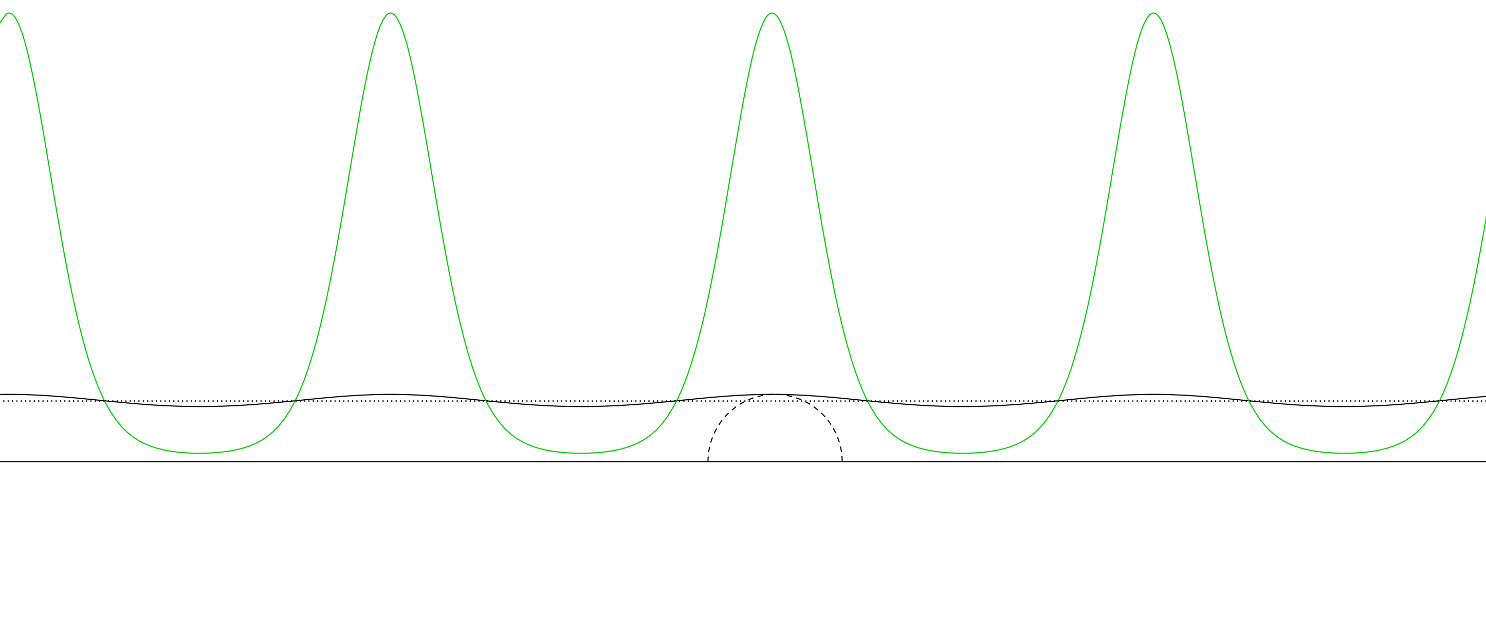
Figure 1. Graphs of $t\mapsto e^{-\cos(t)/10}$ and $t\mapsto e^{-2\cos(t)}$.

Horoconvex functions inherit strong properties from convex functions.

Corollary 2.10.

Any sequence of uniformly bounded horoconvex functions is equi-Lipschitz on any compact set of ${\mathbb{R}}^{2}$.

Moreover, up to extracting a subsequence, the sequence converges uniformly on any compact set to a horoconvex function.

Proof.

Let $C\subset{\mathbb{R}}^{2}$ be a compact set and $(u_{n})$ a sequence of uniformly bounded horoconvex functions. Let $F_{n}(x)=e^{-2u_{n}(x)}+\|x\|^{2}$, which is convex by Proposition 2.6. By [Roc97, 10.4], there exists an $\epsilon>0$ such that for any $x,y\in C$

$$|F_{n}(x)-F_{n}(y)|\leq\frac{\operatorname{max}_{C}F_{n}-\operatorname{min}_{C}F_{n}}{\epsilon}\|x-y\|~{}.$$

As the $u_{n}$ are uniformly bounded, $F_{n}$ are uniformly bounded on $C$, hence there exists a number $A$ satisfying

$$|F_{n}(x)-F_{n}(y)|\leq A\|x-y\|~{}.$$

Using again that the $u_{n}$ are uniformly bounded, and that

$$\left|\|x\|^{2}-\|y\|^{2}\right|\leq 2\left(\sup_{C}\|x\|\right)\|x-y\|~{},$$

we thus obtain that

$$|u_{n}(x)-u_{n}(y)|\leq A^{\prime}\|x-y\|$$

for some $A^{\prime}=A^{\prime}(C)>0$ independent of $n$. So the sequence is equi-Lipschitz on $C$.

Up to extract a subsequence, the sequence of convex functions $(F_{n})$ converge (uniformly on compact sets) to a convex function $F$ [Roc97, Theorem 10.9]). As the $u_{n}$ are uniformly bounded, there exists a positive constant $c$ such that $F_{n}\geq c+\|\cdot\|^{2}$, so $F>\|\cdot\|^{2}$, hence the function

$$u=-\frac{1}{2}\ln(F-\|\cdot\|^{2})$$

is well defined and horoconvex by definition. As $(F_{n})$ converges to $F$ uniformly on compact sets, it follows easily that $u_{n}$ converges to $u$ uniformly on compact sets. ∎

In particular, a horoconvex function is Lipschitz on any compact set. By Rademacher theorem, it is differentiable almost everywhere.

2.3. Induced metric

The length of a curve $c$ in ${\mathbb{H}}^{3}$ is the supremum of the length of all the polygonal paths of ${\mathbb{H}}^{3}$ with vertices on $c$. Equivalently [BBI01, Theorem 2.7.6], if $c$ is Lipschitz (in ${\mathbb{H}}^{3}$), then

$$L(c)=\int\|c^{\prime}\|_{{\mathbb{H}}^{3}}~{}.$$

Let $S$ be a convex surface in ${\mathbb{H}}^{3}$. The (intrinsic) induced metric on $S$ between two points $a,b$ of $S$ is the infimum of the lengths of all the rectifiable Lipschitz curves between $a$ and $b$.

Let $u$ be a horoconvex function. Let $\tilde{d}_{u}$ be the intrinsic metric induced on the horograph of $u$. For simplicity, we will look at metrics onto ${\mathbb{R}}^{2}$ rather than on the surfaces: for $(x,y)\in{\mathbb{R}}^{2}$,

$$d_{u}(x,y):=\tilde{d}_{u}\left(\left(x,e^{-u(x)}\right),\left(y,e^{-u(y)}\right)\right)~{}.$$

Note that, in the upper half space model, notions of locally Lipschitz are equivalent for the metrics of ${\mathbb{H}}^{3}$ and ${\mathbb{R}}^{3}$. Also, the projection from ${\mathbb{R}}^{3}$ onto the horizontal plane is contracting. Hence, a locally Lipschitz curve of ${\mathbb{H}}^{3}$ is projected onto a locally Lipschitz curve of ${\mathbb{R}}^{2}$.

Let $c:[a,b]\rightarrow{\mathbb{R}}^{2}$ be a Lipschitz curve. Let $c_{u}$ be the corresponding curve in the horograph of $u$ i.e. on the graph of $e^{-u}$:

$$c_{u}=\binom{c}{e^{-u\circ c}}~{}.$$

As $u$ is Lipschitz, $c_{u}$ is a Lipschitz curve of ${\mathbb{H}}^{3}$.

Let us denote by $L_{u}(c)$ the length of $c_{u}$ for the metric $\tilde{d}_{u}$ on $S_{u}$. Using the half-space model metric

$$L_{u}(c)=\int_{a}^{b}\frac{\|c_{u}^{\prime}\|_{{\mathbb{R}}^{3}}}{(c_{u})_{3}}=\int_{a}^{b}e^{u\circ c}\left(\|c^{\prime}\|^{2}+((u\circ c)^{\prime})^{2}e^{-2(u\circ c)}\right)^{1/2}$$

i.e.

(4) $$L_{u}(c)=\int_{a}^{b}\left(e^{2u\circ c}\|c^{\prime}\|^{2}+((u\circ c)^{\prime})^{2}\right)^{1/2}~{}.$$

Lemma 2.11.

Let $(u_{n})$ be a uniformly bounded sequence of horoconvex functions. Then on any compact set $K$, $d_{u_{n}}$ are uniformly Lipschitz equivalent to the Euclidean metric: $\exists\lambda_{1},\lambda_{2}>0$ such that

$$\lambda_{1}d_{{\mathbb{R}}^{2}}\leq d_{u_{n}}\leq\lambda_{2}d_{{\mathbb{R}}^{2}}~{}.$$

Moreover, for any Lipschitz curve $c$ contained in $K$,

$$\lambda_{1}L_{{\mathbb{R}}^{2}}(c)\leq L_{u_{n}}(c)\leq\lambda_{2}L_{{\mathbb{R}}^{2}}(c)~{}.$$

Proof.

By construction, for any $x,y\in K$, $d_{u_{n}}(x,y)$ is not less than the distance in ${\mathbb{H}}^{3}$ between the corresponding points on the horograph of $u$. As $K$ is compact and the $u_{n}$ uniformly bounded, the corresponding horographs above $K$ in ${\mathbb{R}}^{3}$ are contained in a hyperbolic ball. There exists a constant $\lambda_{1}$ such that on this ball, $d_{{\mathbb{H}}^{3}}\geq\lambda_{1}d_{{\mathbb{R}}^{3}}$. Also, with evidence, $d_{{\mathbb{R}}^{3}}\geq d_{{\mathbb{R}}^{2}}$. Hence, $d_{{\mathbb{H}}^{3}}\geq\lambda_{1}d_{{\mathbb{R}}^{2}}$. As the length of a Lipschitz curve for $d_{u_{n}}$ is the supremum of the length of shortest polygonal paths [BBI01, 2.3.4,2.4.3] it follows that for any curve $c$ in $K$, $\lambda_{1}L_{{\mathbb{R}}^{2}}(c)\leq L_{u_{n}}(c)$.

On the other hand, for any curve $c$ in $K$, it follows from (4) and from the inequality $\sqrt{a^{2}+b^{2}}\leq|a|+|b|$ that

$$L_{u_{n}}(c)\leq\int_{a}^{b}e^{-u_{n}}\|c^{\prime}\|+|(u\circ c)^{\prime}|$$

and as the $u_{n}$ are uniformly bounded on $K$ by assumption, and also $u_{n}$ are equi-Lipschitz on $K$ by Corollary 2.10, then there exists $\lambda_{2}$ such that

$$L_{u_{n}}(c)\leq\lambda_{2}L_{{\mathbb{R}}^{2}}(c)~{}.$$

∎

The proof of the following lemma mimics the one for convex bodies in Euclidean space [BBI01, p. 358].

Lemma 2.12.

Let $u,v$ be horoconvex such that $u\leq v$ and

$$\delta=\operatorname{sup}_{{\mathbb{R}}^{2}}(v-u)$$

is finite. Then

$$d_{u}\leq d_{v}+2\delta~{}.$$

Proof.

Recall that the Hyperbolic Busemann–Feller Lemma, [BH99, II.2.4] says that the orthogonal projection onto a convex set in ${\mathbb{H}}^{3}$ is contracting. $u\leq v$ implies that the horograph of $v$ is in the exterior of the convex set bounded by the horograph of $u$, so the orthogonal projection is well defined from the horograph of $v$ onto the horograph of $u$. For $a\in{\mathbb{R}}^{2}$, let $p_{\bot}(a)$ be the vertical projection onto ${\mathbb{R}}^{2}$ of the orthogonal projection of $(a,v(a))$ onto the horograph of $u$.

On one hand, Busemann–Feller Lemma implies that

(5) $$d_{u}(p_{\bot}(a),p_{\bot}(b))\leq d_{v}(a,b)~{}.$$

On the other hand, Busemann–Feller Lemma implies that $d_{u}(p_{\bot}(a),a)$ is less than the distance in ${\mathbb{H}}^{3}$ between $(a,v(a))$ and $(a,u(a))$, and this last quantity is less than $\delta$ by assumption, so

(6) $$d_{u}(p_{\bot}(a),a)\leq\delta~{}.$$

The result follows from (5), (6) and the triangle inequality. ∎

3. Proof of Theorem 1.1

Now let $(S,m)$ be a CBB($-1$) metric on the torus. According to Theorem 2.2 there exists a sequence of polyhedral CBB($-1$) metric $m_{n}$ on the torus Gromov–Hausdorff converging to $m$. By Theorem 1.3, for any $n$ there exists a hyperbolic cusp $\mathrm{C}_{n}$ with convex boundary and induced metric on $\partial\mathrm{C}_{n}$ isometric to $m_{n}$.

As mentioned in the introduction, the universal cover $\widetilde{\mathrm{C}_{n}}$ can be isometrically embedded as a convex subset of ${\mathbb{H}}^{3}$ via the developing map $D$. The action of the fundamental group $\pi_{1}(\mathrm{C}_{n})\cong\pi_{1}(T)$ on $\widetilde{\mathrm{C}_{n}}$ by deck transformations yields a representation $\rho:\pi_{1}(T)\to\mathrm{Iso}^{+}({\mathbb{H}}^{3})$. The cusp $\mathrm{C}_{n}$ contains a totally umbilic torus $M$ with Euclidean metric. It follows that the developing map sends the universal cover of $M$ to the horosphere $H$. The group $\rho(\pi_{1}(\mathrm{C}_{n}))=\Gamma_{n}$ acts on $D(\widetilde{M})$ freely with a compact orbit space. The group $\Gamma_{n}$ is a group of parabolic isometries. The surface $S_{n}=\partial D(\widetilde{\mathrm{C}_{n}})$ is convex and globally invariant under the action of $\Gamma_{n}$. It is easy to see that $S_{n}$ is homeomorphic to $H$ via the central projection from the center of $D(\widetilde{M})$. Up to rotations of the hyperbolic space, we normalize the surfaces $S_{n}$ in such a way that the point fixed by $\Gamma_{n}$ is $\infty$ in the half space model. Moreover, choosing a point $x_{0}$ in the universal cover of the torus, up to compose by parabolic and hyperbolic isometries, we consider that the developing maps send $x_{0}$ onto $(0,0,1)_{E}$.

So the surfaces $S_{n}$ are described by horoconvex functions $u_{n}$. We identify $\Gamma_{n}$ with the corresponding lattice in $H={\mathbb{R}}^{2}$. In particular, $u_{n}(\gamma\cdot x)=u_{n}(x)$ for any $\gamma\in\Gamma_{n}$ and $x\in{\mathbb{R}}^{2}$, and the normalization above says that $u_{n}(0)=0$ for any $n$. The quotient of $d_{u_{n}}$ by $\Gamma_{n}$ is isometric to $m_{n}$.

We will prove that $(u_{n},\Gamma_{n})$ converge to some $(u,\Gamma)$ and that the quotient of $d_{u}$ by $\Gamma$ is isometric to $m$. This will prove Theorem 1.1: the wanted cusp is the quotient by $\Gamma$ of the convex side of the horograph of $u$.

3.1. A uniform bound on horographs

From Lemma 2.3, there exists a uniform upper bound $\mathsf{diam}$ of all the diameters of the metrics $m_{n}$.

Lemma 3.1.

1. The sequence $(u_{n})_{n}$ is uniformly bounded.

2. There is a compact set $D\subset{\mathbb{R}}^{2}$ such that for any $y\in{\mathbb{R}}^{2}$ and any $n$, there exists $\gamma\in\Gamma_{n}$ with $\gamma\cdot y\in D$.

Proof.

Recall that all the horographs $S_{n}$ of $u_{n}$ pass through $x_{0}=(0,0,1)_{E}$. Let $b_{n}$ be the set of points on $S_{n}$ at distance $\leq$ $\mathsf{diam}$ from $(0,0,1)_{E}$ in the intrinsic metric of $S_{n}$. Then as the distance on $S_{n}$ is greater than the extrinsic distance of ${\mathbb{H}}^{3}$, all the $b_{n}$ are contained in a same hyperbolic ball $B$.

In the half space model, let $D$ be the projection of the ball $B$ onto the horizontal plane passing through the origin. Observe that $D=\overline{B^{{\mathbb{R}}^{2}}_{\delta}(0)}$ is a Euclidean closed ball centred at the origin of ${\mathbb{R}}^{2}$. As $B$ is contained between two horospheres centred at $\infty$ (i.e. two horizontal planes) the horofunctions $u_{n}$ are uniformly bounded on $D$, say $c_{1}<u_{n}<c_{2}$. Now by construction, for any $y\in{\mathbb{R}}^{2}$, there exists $\gamma\in\Gamma_{n}$ such that $\gamma\cdot y\in D$. Hence $c_{1}<u_{n}(\gamma\cdot y)=u_{n}(y)<c_{2}$. ∎

3.2. Convergence of groups

Lemma 3.2.

There exists a sequence $(a_{n},b_{n})_{n}$ of generators of $\Gamma_{n}$ that converges in ${\mathbb{R}}^{2}$ (up to extract a subsequence) to two linearly independent non-zero vectors $a$ and $b$. (Here we identify an element of $\gamma$ of $\Gamma_{n}$ with the vector $\gamma\cdot 0$ of ${\mathbb{R}}^{2}$.)

Proof.

Let us choose generators $(a_{n},b_{n})$ of $\Gamma_{n}$ which are contained in $\overline{B^{{\mathbb{R}}^{2}}_{3\delta}(0)}$, that is possible by the second item of Lemma 3.1. Since $\overline{B^{{\mathbb{R}}^{2}}_{3\delta}(0)}$ is compact, up to take a subsequence we get the existence of two vectors $a,b\in{\mathbb{R}}^{2}$ such that $a_{n}\to a$ and $b_{n}\to b$ as $n\to\infty$.

Suppose that either one of the vectors $a$ or $b$ is zero, or that they are parallel. By continuity we necessarily have that the area of the parallelogram with side $a_{n}$ and $b_{n}$ tends to zero, as $n\to\infty$. In turn, this means that the area of a fundamental domain of ${\mathbb{R}}^{2}$ for the action of $\Gamma_{n}$ tend to zero as $n\to\infty$. Applying Lemma 2.11 with $K=\overline{B^{{\mathbb{R}}^{2}}_{3\delta}(0)}$, by Proposition 3.1.4 in [AT04], the two dimensional Hausdorff measure of $m_{n}$ tends to zero, thus contradicting Theorem 2.4. ∎

3.3. Construction of the solution

By Corollary 2.10 and Lemma 3.1, up to extract a subsequence, the sequence $(u_{n})$ converges to a horoconvex function $u$, uniformly on any compact set.

Let $a,b\in{\mathbb{R}}^{2}$ given by Lemma 3.2, and define $\Gamma\subset\operatorname{Iso}({\mathbb{R}}^{2})$ as the direct product of $\left\langle a\right\rangle$ and $\left\langle b\right\rangle$. Since $a$ and $b$ are linearly independent vectors, ${\mathbb{R}}^{2}/\Gamma$ is a torus.

Lemma 3.3.

The function $u$ is $\Gamma$-invariant.

Proof.

Let $y\in{\mathbb{R}}^{2}$ and $\gamma\in\Gamma$ such that $\gamma y=y+ka+k^{\prime}b$, where $k,k^{\prime}\in{\mathbb{Z}}$. Then, for every $\epsilon>0$

$$|u(\gamma y)-u(y)| =|u(y+ka+k^{\prime}b)-u(y)|$$

(7) $$\leq|u(y+ka+k^{\prime}b)-u_{n}(y+ka+k^{\prime}b)|$$

(8) $$+|u_{n}(y+ka+k^{\prime}b)-u_{n}(y+ka_{n}+k^{\prime}b_{n})|$$

(9) $$+|u_{n}(y+ka_{n}+k^{\prime}b_{n})-u_{n}(y)|$$

(10) $$+|u_{n}(y)-u(y)|<\epsilon$$

for $n$ large enough. In fact $k(a-a_{n})+k^{\prime}(b-b_{n})\to 0$ as $n\to\infty$, and as the $u_{n}$ are equi-Lipschitz on a sufficiently large compact set the absolute value at line (8) is smaller than $\epsilon/4$ for $n$ large enough. Moreover, the absolute value at line (9) is zero for every $n$ by the $\Gamma_{n}$-invariance of $u_{n}$, and the absolute value at lines (7) and (10) are smaller then $\epsilon/4$ for $n$ large enough by the uniform convergence of the $u_{n}$. Since $\epsilon>0$ is arbitrary, this concludes the proof. ∎

3.4. Convergence of metrics

In the preceding section, we have constructed a pair $(u,\Gamma)$. It remains to check that the induced metric $m_{u}$ on $({\mathbb{R}}^{2},d_{u})/\Gamma$ is isometric to $(T,m)$. Basically, one has to check that if the sequence $(u_{n})$ converges, then the sequence of induced metric converges. In the remaining of this section we will prove the following result, that ends the proof of the theorem, because on compact metric spaces, uniform convergence imply Gromov–Hausdorff convergence, and the Gromov–Hausdorff limit is unique.

Proposition 3.4.

The sequence $(m_{n})$ uniformly converges to $m$.

Lemma 3.5.

Let $K\subset{\mathbb{R}}^{2}$ be compact. Then

$$E(K)=\operatorname{closure}\left(\cup_{x\in K}\cup_{n}\{y|d_{u_{n}}(x,y)\leq\mathsf{diam}\}\right)$$

is compact.

Proof.

We have

$$d_{{\mathbb{H}}^{3}}\left(\left(x,e^{-u_{n}(x)}\right),\left(y,e^{-u_{n}(y)}\right)\right)\leq d_{u_{n}}(x,y)\leq\mathsf{diam}~{},$$

but [Rat06, 4.6.1]

$$\cosh d_{{\mathbb{H}}^{3}}\left(\left(x,e^{-u_{n}(x)}\right),\left(y,e^{-u_{n}(y)}\right)\right)=1+\frac{\|x-y\|^{2}}{2e^{-u_{n}(x)}e^{-u_{n}(y)}}$$

so

$$\|x-y\|\leq\sqrt{2}e^{-c}\sqrt{\cosh(\mathsf{diam})-1}$$

where $c$ is the uniform lower bound of the $u_{n}$. The result follows because $K$ is compact.

∎

Corollary 3.6.

Let $K\subset{\mathbb{R}}^{2}$ be compact. Let $\mathcal{L}(K)$ be the set of shortest paths for any $d_{n}$ between points of $K$ (we don’t ask the shortest path to be contained in $K$). Then there exists a constant $\alpha$ such that $\forall c\in\mathcal{L}(K)$, $L_{{\mathbb{R}}^{2}}(c)\leq\alpha$.

Proof.

By Lemma 2.11 applied to $K$, for any $x,y\in K$,

$$d_{u_{n}}(x,y)\leq\lambda_{2}(K)\operatorname{diam}(K)~{}.$$

Let $c$ be a shortest path for $u_{n}$ between $x$ and $y$, so that $L_{u_{n}}(c)=d_{u_{n}}(x,y)$.

The shortest path is contained in the compact set $E(K)$ given by Lemma 3.5, so by Lemma 2.11 again, but applied to $E(K)$, $L_{{\mathbb{R}}^{2}}(c)\leq\frac{\lambda_{2}(K)}{\lambda_{1}(E(K))}\operatorname{diam}(K)$. ∎

Lemma 3.7.

Let $K\subset{\mathbb{R}}^{2}$ be compact. Then $d_{u_{n}}$ uniformly converge to $d_{u}$ on $K$.

Proof.

Let $\epsilon>0$. As $u_{n}$ uniformly converge to $u$, for $n$ sufficiently large, $u\leq u_{n}+\epsilon$, so by Lemma 2.12

$$d_{u}\leq d_{u_{n}+\epsilon}+4\epsilon~{}.$$

Let $x,y\in K$ and let $c$ be a shortest path for $u_{n}$ between $x$ and $y$. Then

$$d_{u_{n}+\epsilon}(x,y)\leq L_{u_{n}+\epsilon}(c)$$

and from (4), the fact that the $u_{n}$ are uniformly bounded and Corollary 3.6, there exists a constant $\beta$ depending only on $K$ such that

$$L_{u_{n}+\epsilon}(c)\leq L_{u_{n}}(c)+\sqrt{|e^{2\epsilon}-1|}\beta(K)$$

and as $L_{u_{n}}(c)=d_{u_{n}}(x,y)$ we obtain

$$d_{u}(x,y)-d_{u_{n}}(x,y)\leq 4\epsilon+\sqrt{|e^{2\epsilon}-1|}\beta(K)~{}.$$

Exchanging the role of $u$ and $u_{n}$, we finally obtain

$$|d_{u}(x,y)-d_{u_{n}}(x,y)|\leq 4\epsilon+\sqrt{|e^{2\epsilon}-1|}\beta(K)~{}.$$

∎

Remark 3.8.

A result of A.D. Alexandrov gives a weaker convergence of the induced metrics for any convex surfaces converging in the Hausdorff sense to a convex surface in the hyperbolic space, see [Slu].

Let $\tilde{\varphi}_{n}$ be the linear isomorphism sending $a$ to $a_{n}$ and $b$ to $b_{n}$. Hence clearly, for any $\gamma\in\Gamma$,

$$\tilde{\varphi}_{n}(\gamma\cdot x)=\tilde{\varphi}_{n}(\gamma)\cdot\tilde{\varphi}_{n}(x)$$

where $\gamma$ is considered as a vector of ${\mathbb{R}}^{2}$. The map $\tilde{\varphi}_{n}$ descends to a homeomorphism $\varphi_{n}$ between ${\mathbb{R}}^{2}/\Gamma$ and ${\mathbb{R}}^{2}/\Gamma_{n}$.

Lemma 3.9.

Let $K\subset\mathbb{R}^{2}$ a compact set. Then on $K$,

$$x\mapsto d_{u_{n}}(\tilde{\varphi}_{n}(x),x)$$

uniformly converge to zero and $d_{u_{n}}(\tilde{\varphi}_{n}(x),\tilde{\varphi}_{n}(y))$ uniformly converge to $d_{u}(x,y)$.

Proof.

$\tilde{\varphi}_{n}$ converge to the identity map, uniformly on any compact for the Euclidean metric. The first result follows from Lemma 2.11. The second result follows easily from the first one, the triangle inequality and Lemma 3.7. ∎

Lemma 3.10.

There exists a compact set $K\subset{\mathbb{R}}^{2}$ such that for any $n$, for any $p,q$ in the torus, a lift of a shortest path for $m_{n}$ between $p$ and $q$ is contained in $K$.

Proof.

Let $K=E(D)$, where $D$ is the compact set obtained in Lemma 3.1. By definition of $D$, there exists a lift $x$ of $p$ in $D$. By construction of $K$, the ball for $d_{n}$ centred at $x$ with radius $m_{n}(p,q)$ is contained in $K$. ∎

Let $C$ be the closure of $\cup_{n}\tilde{\varphi}_{n}(K)$, where $K$ is given by Lemma 3.10. $C$ is a compact set.

Lemma 3.11.

For any $\nu>0$, if $n$ is sufficiently large, for any $p,q\in T$, if $x$ and $y$ are respective lifts to the set $C$ defined above, if $d_{u}(x,y)=m(p,q)$, then

$$m_{n}(\varphi_{n}(p),\varphi_{n}(q))\leq d_{u_{n}}(\tilde{\varphi}_{n}(x),\tilde{\varphi}_{n}(y))\leq m_{n}(\varphi_{n}(p),\varphi_{n}(q))+\nu~{}.$$

Proof.

As $d_{u}(x,y)=m(p,q)$, for any $\gamma\in\Gamma$,

$$d_{u}(x,\gamma\cdot y)\geq d_{u}(x,y)~{}.$$

By Lemma 3.9, uniformly on $C$, if $n$ is sufficiently large,

$$d_{u_{n}}(\tilde{\varphi}_{n}(x),\tilde{\varphi}_{n}(\gamma)\cdot\tilde{\varphi}_{n}(y))+\nu\geq d_{u_{n}}(\tilde{\varphi}_{n}(x),\tilde{\varphi}_{n}(y))~{}.$$

The result follows because $m_{n}(\varphi_{n}(p),\varphi_{n}(q))$ is the minimum on $\Gamma$ of all the $d_{u_{n}}(\tilde{\varphi}_{n}(x),\tilde{\varphi}_{n}(\gamma)\cdot\tilde{\varphi}_{n}(y))$. ∎

Proof of Proposition 3.4.

Let $\epsilon>0$. For any $p,q\in T$, with the notations of Lemma 3.11, for $n$ large enough,

$$m_{n}(\varphi_{n}(p),\varphi_{n}(q))-m(p,q)$$

$$\leq d_{u_{n}}(\tilde{\varphi}_{n}(x),\tilde{\varphi}_{n}(y))-d_{u}(x,y)~{}.$$

By Lemma 3.9 applied on the compact set $C$, for $n$ sufficiently large, the last quantity above is less than $\epsilon$, independently of $x$ and $y$. For the same reasons, the same conclusion holds for

$$m(p,q)-m_{n}(\varphi_{n}(p),\varphi_{n}(q))$$

$$\leq d_{u}(x,y)-d_{u_{n}}(\tilde{\varphi}_{n}(x),\tilde{\varphi}_{n}(y))+\nu~{}.$$

∎

References

- [AKP] S. Alexander, V. Kapovitch, and A. Petrunin. Alexandrov geometry. In preparation. Draft version available.
- [AKP08] S. Alexander, V. Kapovitch, and A. Petrunin. An optimal lower curvature bound for convex hypersurfaces in Riemannian manifolds. Illinois J. Math., 52(3):1031–1033, 2008.
- [Ale06] A. D. Alexandrov. A. D. Alexandrov selected works. Part II. Chapman & Hall/CRC, Boca Raton, FL, 2006. Intrinsic geometry of convex surfaces, Edited by S. S. Kutateladze, Translated from the Russian by S. Vakhrameyev.
- [AT04] L. Ambrosio and P. Tilli. Topics on analysis in metric spaces, volume 25 of Oxford Lecture Series in Mathematics and its Applications. Oxford University Press, Oxford, 2004.
- [BBI01] D. Burago, Y. Burago, and S. Ivanov. A course in metric geometry, volume 33 of Graduate Studies in Mathematics. American Mathematical Society, Providence, RI, 2001.
- [BGP92] Yu. Burago, M. Gromov, and G. Perel′man. A. D. Aleksandrov spaces with curvatures bounded below. Uspekhi Mat. Nauk, 47(2(284)):3–51, 222, 1992.
- [BH37] W. Blaschke and G. Herglotz. Über die Verwirklichung einer geschlossenen Fläche mit vorgeschriebenem Bogenelement im Euklidischen Raum. Sitzungsber. Bayer. Akad. Wiss., Math.-Naturwiss. Abt., (2):229–230, 1937.
- [BH99] M. Bridson and A. Haefliger. Metric spaces of non-positive curvature, volume 319 of Grundlehren der Mathematischen Wissenschaften [Fundamental Principles of Mathematical Sciences]. Springer-Verlag, Berlin, 1999.
- [BI08] A. Bobenko and I. Izmestiev. Alexandrov’s theorem, weighted Delaunay triangulations, and mixed volumes. Ann. Inst. Fourier (Grenoble), 58(2):447–505, 2008.
- [CEG06] R. D. Canary, D. B. A. Epstein, and P. L. Green. Notes on notes of Thurston [mr0903850]. In Fundamentals of hyperbolic geometry: selected expositions, volume 328 of London Math. Soc. Lecture Note Ser., pages 1–115. Cambridge Univ. Press, Cambridge, 2006. With a new foreword by Canary.
- [CX15] J.-E. Chang and L. Xiao. The Weyl problem with nonnegative Gauss curvature in hyperbolic space. Canad. J. Math., 67(1):107–131, 2015.
- [FI09] F. Fillastre and I. Izmestiev. Hyperbolic cusps with convex polyhedral boundary. Geom. Topol., 13(1):457–492, 2009.
- [Fil07] F. Fillastre. Polyhedral realisation of hyperbolic metrics with conical singularities on compact surfaces. Ann. Inst. Fourier (Grenoble), 57(1):163–195, 2007.
- [Gro86] M. Gromov. Partial differential relations, volume 9 of Ergebnisse der Mathematik und ihrer Grenzgebiete (3) [Results in Mathematics and Related Areas (3)]. Springer-Verlag, Berlin, 1986.
- [GSS09] B. Guan, J. Spruck, and M. Szapiel. Hypersurfaces of constant curvature in hyperbolic space. I. J. Geom. Anal., 19(4):772–795, 2009.
- [IRV15] J. Itoh, J. Rouyer, and C. Vîlcu. Moderate smoothness of most Alexandrov surfaces. Internat. J. Math., 26(4):1540004 (14 pages), 2015.
- [Izm08] I. Izmestiev. A variational proof of Alexandrov’s convex cap theorem. Discrete Comput. Geom., 40(4):561–585, 2008.
- [Izm13] I. Izmestiev. Infinitesimal rigidity of smooth convex surfaces through the second derivative of the Hilbert-Einstein functional. Dissertationes Math. (Rozprawy Mat.), 492:58, 2013.
- [Lab92] F. Labourie. Métriques prescrites sur le bord des variétés hyperboliques de dimension . J. Differential Geom., 35(3):609–626, 1992.
- [Pog73] A. V. Pogorelov. Extrinsic geometry of convex surfaces. American Mathematical Society, Providence, R.I., 1973. Translated from the Russian by Israel Program for Scientific Translations, Translations of Mathematical Monographs, Vol. 35.
- [Rat06] J. Ratcliffe. Foundations of hyperbolic manifolds, volume 149 of Graduate Texts in Mathematics. Springer, New York, second edition, 2006.
- [Ric12] T. Richard. Ricci flow without upper bounds on the curvature and the geometry of some metric spaces. Theses, Université de Grenoble, September 2012.
- [Roc97] R. Rockafellar. Convex analysis. Princeton Landmarks in Mathematics. Princeton University Press, Princeton, NJ, 1997. Reprint of the 1970 original, Princeton Paperbacks.
- [RS94] H. Rosenberg and J. Spruck. On the existence of convex hypersurfaces of constant Gauss curvature in hyperbolic space. J. Differential Geom., 40(2):379–409, 1994.
- [RW98] T. Rockafellar and R. Wets. Variational analysis, volume 317 of Grundlehren der Mathematischen Wissenschaften [Fundamental Principles of Mathematical Sciences]. Springer-Verlag, Berlin, 1998.
- [Sch06] J.-M. Schlenker. Hyperbolic manifolds with convex boundary. Invent. Math., 163(1):109–169, 2006.
- [Slu] D. Slutskiy. Compact domains with prescribed convex boundary metrics in quasi-Fuchsian manifolds. arXiv:1405.1650.
- [Slu14] D. Slutskiy. Polyhedral metrics on the boundaries of convex compact quasi-Fuchsian manifolds. C. R. Math. Acad. Sci. Paris, 352(10):831–834, 2014.