Differences in the quasiparticle dynamics for one-band and three-band cuprate models

Abstract

We study the quasiparticles of the one-band $t$-$J$ and $t$-$t^{\prime}$-$t^{\prime\prime}$-$J$ models using a variational approximation that includes spin fluctuations in the vicinity of the hole. We explain why the spin fluctuations and the longer range hopping have complementary contributions to the quasiparticle dynamics, and thus why both are essential to obtain a dispersion in agreement with that measured experimentally. This is very different from the three-band Emery model in the strongly-correlated limit, where the same variational approximation shows that spin fluctuations have a minor effect on the quasiparticle dynamics. This difference proves that these one-band and three-band models describe qualitatively different quasiparticles, and therefore they they cannot both be suitable to describe the physics of underdoped cuprates.

I Introduction

Nearly three decades after their discovery Bend , the high-temperature cuprate superconductors have so far eluded a comprehensive explanation. These layered materials contain CuO₂ layers, which are antiferromagnetic insulators in the undoped limit and become superconducting upon doping RMP_reviews . The hole-doped side shows a more robust superconductivity, extending to higher temperatures and over a wider range of dopings. The first step towards deciphering the mechanism of superconductivity in these compounds is a proper description of the motion of these holes in the CuO₂ layer – this has become one of the most studied problems in condensed matter theory RMP_reviews ; Kane89 . Its solution should elucidate the nature of the quasiparticles that eventually bind together into the pairs that facilitate the superconducting state.

Despite significant effort, even what is the minimal model that correctly describes this low-energy quasiparticle is still not clear. There is general agreement that the parent compounds are charge-transfer insulators Zaanen , and wide consensus that most of their low-energy physics is revealed by studies of a single CuO₂ layer, modeled in terms of Cu $3d_{x^{2}-y^{2}}$ and O $2p$ orbitals. Because only ligand $2p$ orbitals hybridize with the $3d_{x^{2}-y^{2}}$ orbitals, it is customary to ignore the other O $2p$ orbitals; this leads to the well-known three-band Emery model Emery .

However, the Emery model is perceived as too complicated to study so it is often further simplified to a one-band $t$-$J$ model that describes the dynamics of a Zhang-Rice singlet (ZRS) Zhang ; George . We known that the $t$-$J$ model with only nearest-neighbor (nn) hopping $t$ is certainly not the correct model because it predicts a nearly flat quasiparticle energy along $(0,\pi)-(\pi,0)$, unlike the substantial dispersion found experimentally Wells ; Leung95 ; Damascelli . However, its extension with longer range hopping, the $t$-$t^{\prime}$-$t^{\prime\prime}$-$J$ model, was shown to reproduce the correct dispersion Leung97 for values of the 2^nd and 3^rd nn hoppings in rough agreement with those estimated from density functional theory ok and cluster calculations eskes . Taking this agreement as proof that this is the correct model, both the $t$-$J$ model and its parent, the Hubbard model amol , have been studied very extensively in the context of cuprate physics.

Here we show that the quasiparticle of the $t$-$t^{\prime}$-$t^{\prime\prime}$-$J$ model is qualitatively different from that of the $U_{dd}\rightarrow\infty$ limit of the three-band Emery model comment . While both models predict a dispersion in quantitative agreement with that measured experimentally (for suitable values of the parameters), the factors controlling the quasiparticle dynamics are very different. It has long been known that both the longer-range hopping and the spin fluctuations play a key role in the dynamics of the quasiparticle of the $t$-$t^{\prime}$-$t^{\prime\prime}$-$J$ model. Here we use a non-perturbative variational method, which agrees well with available exact diagonalization (ED) results, to show that spin-fluctuations and longer-range hopping control the quasiparticle dispersion in different parts of the Brillouin zone, and to explain why. In contrast, using the same variational approach, it was recently argued that spin fluctuations play no role in the dispersion of the quasiparticle of the $U_{dd}\rightarrow\infty$ limit of the Emery model Hadi . This claim is supported by additional results we present here.

This major difference in the role played by spin fluctuations in determining the quasiparticle dynamics shows that these models do not describe the same physics. This suggests that the $t$-$t^{\prime}$-$t^{\prime\prime}$-$J$ model is not suitable for the study of cuprates in the hole-doped regime, although it and related one-band models may be valid in the electron-doped regime. As we argue below, it may be possible to “fix” one-band models by addition of other terms, although we do not expect this to be a fruitful enterprise. Instead, we believe that what is needed is a concerted effort to understand the predictions of the Emery model. Our results in Ref. Hadi and here that spin fluctuations of the AFM background do not play a key role in the quasiparticle dynamics of this three-band model, contrary to what was believed to be the case based on results from one-band models, should simplify this task.

The article is organized as follows. In Section II we review the three-band Emery model and briefly discuss the emergence of the one-band and simplified three-band models in the asymptotic limit of strong correlations on the Cu sites. Section III describes the variational method, which consists in keeping a limited number of allowed magnon configurations in the quasiparticle cloud. Section IV presents our results for both one- and three-band models, and their interpretation. Finally, Section V contains a summary and a detailed discussion of the implications of these results.

II Models

A widely accepted starting point for the description of a CuO₂ layer is the three-band Emery model Emery :

$$\mathcal{H}=T_{pp}+T_{pd}+\Delta_{pd}\sum_{i\in{\rm O},\sigma}n_{i,\sigma}\\ +U_{pp}\sum_{i\in{\rm O}}n_{i,\downarrow}n_{i,\uparrow}+U_{dd}\sum_{i\in{\rm Cu}}n_{i,\downarrow}n_{i,\uparrow}.$$ (1)

The sets ${\rm O}$ and ${\rm Cu}$ contain the ligand O $2p$ and the Cu $3d_{x^{2}-y^{2}}$ orbitals respectively, sketched in Fig. 1(a). For ${i\in{\rm O}}$, $n_{i,\sigma}=p^{\dagger}_{i,\sigma}p_{i,\sigma}$ is the number of spin-$\sigma$ holes in that $2p$ orbital. Similar notation is used for the $3d$ orbitals, their hole creation operators being $d^{\dagger}_{i,\sigma}$, $i\in{\rm Cu}$.

$T_{pp}$ is the kinetic energy of the holes moving on the O sublattice, described by a Hamiltonian with first ($t_{pp}$) and second ($t^{\prime}_{pp}$) nearest-neighbour (nn) hopping:

$$T_{pp}=t_{pp}\sum_{i\in{\rm O},{\boldsymbol{\delta}},\sigma}r_{\boldsymbol{\delta}}p^{\dagger}_{i,{\sigma}}p_{i+{\boldsymbol{\delta}},\sigma}\\ -t^{\prime}_{pp}\sum_{i\in{\rm O},\sigma}p^{\dagger}_{i,\sigma}(p_{i-{\boldsymbol{\epsilon}},\sigma}+p_{i+{\boldsymbol{\epsilon}},\sigma}).$$ (2)

The lattice constant is set to $a=1$. The vectors ${\boldsymbol{\delta}}=\pm(0.5,0.5),\pm(0.5,-0.5)$ are the distances between any O and its four nn O sites, and $r_{{\boldsymbol{\delta}}}=\pm 1$ sets the sign of each nn $pp$ hopping integral in accordance with the overlap of the $2p$ orbitals involved, see Fig. 1(a). Next nn hopping is included only between O $2p$ orbitals pointing toward a common bridging Cu, separated by ${\boldsymbol{\varepsilon}}=(1,0)$ or $(0,1)$; hybridization with the $4s$ orbital of the bridging Cu further boosts the value of this hopping integral.

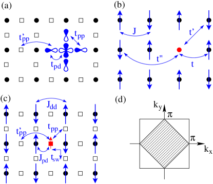
Figure 1: (color online) (a) Sketch of the CuO₂ layer, with O are marked by squares and Cu marked by circles. The relevant orbitals are drawn at a few sites. The arrows indicate the hopping terms included in the three-band Emery model; (b) Sketch of the one-band $t$-$t^{\prime}$-$t^{\prime\prime}$-$J$ model. Cu sites host spin degrees of freedom, except at sites where a Zhang-Rice singlet is centered (red circle). The arrows indicate the various terms in this Hamiltonian; (c) Sketch of the $U_{dd}\rightarrow\infty$ limit of the Emery model. Cu sites host spin degrees of freedom but the doped holes (red filled square) move on the O lattice. The arrows indicate the various terms in this Hamiltonian; (d) The full Brillouin zone of the CuO₂ lattice (the outer square) which encloses the magnetic Brillouin zone (shaded).

$T_{pd}$ is the kinetic energy of holes moving between neighbour Cu and O orbitals:

$$T_{pd}=t_{pd}\sum_{i\in{\rm Cu},\bf u,\sigma}r_{\bf u}d^{\dagger}_{i,{\sigma}}p_{i+\bf u,\sigma}+h.c.,$$ (3)

where ${\bf u}=(\pm 0.5,0),(0,\pm 0.5)$ are the distances between a Cu and its four nn O sites, and $r_{\bf u}$ are the signs of the overlaps of the corresponding orbitals. It is this term that provides the main justification for ignoring the other sets of $2p$ orbitals, because symmetry forbids hopping of Cu holes from $3d_{x^{2}-y^{2}}$ orbitals into the non-ligand O orbitals. We further discuss this assumption below.

$\Delta_{pd}$ is the charge transfer energy which ensures that in the parent compound the O $2p$ orbitals are fully occupied (i.e. contain no holes). Finally, $U_{pp}$ and $U_{dd}$ are the Hubbard repulsion in the $2p$ and $3d$ orbitals, respectively. Longer range Coulomb interaction between holes on O and Cu can also be added, but for the single doped-hole problem analyzed here, it leads to a trivial energy shift.

Strong correlations due to the large $U_{dd}$, combined with the big Hilbert space with its three-orbitals basis, and the need for a solution for a hole concentration equal (in the parent compound) or larger (in the hole doped case) than one per Cu, make this problem very difficult to solve. While progress is been made with a variety of techniques 3band (which however have various restrictions, such as rather high-temperatures and/or small clusters for quantum Monte Carlo methods, and/or additional approximations, such as setting $t_{pp}=0$ for convenience), it is far more customary to further simplify this model before attempting a solution.

A reasonable way forward is to use the limit $U_{dd}\rightarrow\infty$ to forbid double occupancy of the $3d$ orbitals. As a result, in the undoped ground-state there is one hole per Cu. Virtual hopping processes lead to antiferromagnetic (AFM) superexchange between the resulting spin degrees of freedom, so that the parent compound is a Mott insulator with long-range AFM order comm0 .

Upon doping, holes enter the O band and the issue is how to accurately describe their dynamics as they interact with the spins at the Cu sites. Here we compare two such descriptions for the single doped hole case.

II.1 One-band models

In their seminal work Zhang , Zhang and Rice argued that the doped hole occupies the linear combination of the four $O$ 2p ligand orbitals surrounding a central Cu, that has the same ${x^{2}-y^{2}}$ symmetry like the Cu $3d$ orbital hosting the spin. Furthermore, exchange locks the two holes in a low-energy Zhang-Rice singlet (ZRS). They also argued that the dynamics of this composite object, which combines charge and spin degrees of freedom, is well captured by the one-band model:

$${\cal{H}}={\cal P}\left[\hat{T}+\hat{T^{\prime}}+\hat{T}^{\prime\prime}\right]{\cal P}+\mathcal{H}_{\mathrm{AFM}}.$$ (4)

The first term describes the hopping of the ZRS (marked in Fig. 1(b) by the “missing spin” locked in the ZRS) on the square lattice of Cu sites that hosts it. Originally only nn hopping $T$ was included: $\hat{T}=t\sum_{\langle i,j\rangle}d^{\dagger}_{i,\sigma}d_{j,\sigma}+h.c.$, with $i,j\in{\rm Cu}$. The projector ${\cal P}$ removes doubly occupied states, therefore this term allows only Cu spins neighboring the ZRS to exchange their location with the ZRS. This mimics the more complex reality of the doped hole moving on the O sublattice and forming ZRS with different Cu spins.

Although in Ref. Zhang it was argued that only nn ZRS hoping is important, longer-range 2nd ($\hat{T}^{\prime}$) and 3rd ($\hat{T}^{\prime\prime}$) nn hopping was later added the model on a rather ad-hoc basis. As discussed below, this is needed in order to find a quasiparticle dispersion similar to that measured experimentally. These terms are defined similarly to $\hat{T}$ with hopping integrals $t^{\prime}$ and $t^{\prime\prime}$, respectively. For cuprates, $t^{\prime}/t\sim-0.3,t^{\prime\prime}/t\sim 0.2$ are considered to be representative values ts0 ; ts , in agreement with various estimates ok ; eskes . In the following, we refer to this as the $t$-$t^{\prime}$-$t^{\prime\prime}$-$J$ model, whereas if $t^{\prime}=t^{\prime\prime}=0$ we call it the $t$-$J$ model.

The term $\mathcal{H}_{\mathrm{AFM}}=J\sum_{\langle i,j\rangle}{\bf S}_{i}\cdot{\bf S}_{j}$ describes the nn AFM superexchange between the other Cu spins ${\bf S}_{i}$, with $J/t\sim 0.3$ for cuprates ts . It leads to AFM order in the undoped system comm0 , and also controls the energy of the cloud of magnons that are created in the vicinity of the ZRS, as it moves through the magnetic background.

The $t$-$J$ model also emerges as the $U\rightarrow\infty$ limit of the Hubbard model amol , but with additional terms of order $J$. One of them, $-J/4\sum_{\langle i,j\rangle}n_{i}n_{j}$, gives trivial energy shifts for both the undoped and the single-hole doped cases of interest to us in this work, so its presence can be safely ignored in this context. More interesting is the so-called three-site term ${\cal P}\hat{T}_{3s}{\cal P}$ 3site , where

$$\hat{T}_{3s}=\frac{J}{4}\sum_{i\in{\rm Cu},\sigma}\sum_{\boldsymbol{\epsilon}\neq\boldsymbol{\epsilon}^{\prime}}(d^{\dagger}_{i+\boldsymbol{\epsilon}^{\prime},\sigma}n_{i,-\sigma}d_{i+\boldsymbol{\epsilon},\sigma}\\ -d^{\dagger}_{i+\boldsymbol{\epsilon}^{\prime},\sigma}d^{\dagger}_{i,-\sigma}d_{i,\sigma}d_{i+\boldsymbol{\epsilon},-\sigma})$$ (5)

describes ZRS hopping through an intermediate Cu site and permits spin swapping with the spin at this intermediate site. As shown below, this term influences the quasiparticle dispersion but it is not clear that it should be included in the one-band model, because the original Hamiltonian is the Emery, not the Hubbard, model.

In fact, a perturbational derivation of the low-energy Hamiltonian obtained by projecting the three-band model onto ZRS states reveals a much more complicated Hamiltonian than the $t$-$t^{\prime}$-$t^{\prime\prime}$-$J$ model, with many other terms ALigia . We are not aware of a systematic study of their impacts, but their presence underlies one important issue with this approach: the hoped-for simplification due to the significant decrease in the size of the Hilbert space comes at the expense of a Hamiltonian whose full expression ALigia is very complicated. Using instead simpler versions like the $t$-$t^{\prime}$-$t^{\prime\prime}$-$J$ model may result in qualitatively different physics than that of the full one-band model. Here we argue that this is indeed the case.

II.2 Simplified three-band model

An alternative is to begin at the same starting point, i.e. the limit $U_{dd}\rightarrow\infty$ resulting in spin degrees of freedom at the Cu sites. However, the O sublattice on which the doped hole moves is kept in the model, not projected out like in the one-band approach, see Fig. 1(c). This leads to a bigger Hilbert space than for one-band models (yet smaller than for the Emery model) but because spin and charge degrees of freedom are no longer lumped together, the resulting low-energy Hamiltonian is simpler and makes it easier to understand its physics.

The effective model for a layer with a single doped hole, which for convenience we continue to call ”the three-band model” although it is its $U_{dd}\rightarrow\infty$ approximation, was derived in Ref. Bayo and reads:

$$\mathcal{H}_{\mathrm{eff}}=\mathcal{H}_{\mathrm{AFM}}+\mathcal{H}_{J_{pd}}+T_{pp}+T_{\mathrm{swap}}.$$ (6)

The meaning of its terms is as follows:

$$\mathcal{H}_{\mathrm{AFM}}=J_{dd}\sum_{\langle i,j\rangle^{\prime}}{\bf S}_{i}\cdot{\bf S}_{j}$$

is again the nn AFM superexchange between the Cu spins ${\bf S}_{i}$, so $J_{dd}\equiv J$ of the one-band models. The main difference is indicated by the presence of the prime, which reflects the absence of coupling for the pair that has the doping hole on their bridging O. The next term,

$$\mathcal{H}_{J_{pd}}=J_{pd}\sum_{i\in O,{\bf u}}{\bf s}_{i}\cdot{\bf S}_{i+{\bf u}}$$

is the exchange of the hole’s spin ${\bf s}_{i}={1\over 2}\sum_{\alpha,\beta}p^{\dagger}_{i\alpha}{\boldsymbol{\sigma}}_{\alpha\beta}p_{i\beta}$ with its two nn Cu spins. It arises from virtual hopping of a hole between a Cu and the O hosting the doped hole.

Like in Eq. (1), $T_{pp}$ is the kinetic energy of the doping hole as it moves on the O sublattice. It is supplemented by $T_{\mathrm{swap}}$ which describes effective hopping mediated by virtual processes where a Cu hole hops onto an empty O orbital, followed by the doping hole filling the now empty Cu state Bayo . This results in effective nn or next nn hopping of the doped hole, with a swapping of its spin with that of the Cu involved in the process. The explicit form of this term is:

$$T_{\mathrm{swap}}=-t_{sw}\sum_{i\in{\rm Cu},{\bf u\neq u^{\prime}}}\sum_{\sigma,\sigma^{\prime}}s_{\bf u-u^{\prime}}p^{\dagger}_{i+\bf u,{\sigma}}p_{i+\bf u^{\prime},\sigma^{\prime}}|i_{\sigma^{\prime}}\rangle\langle i_{\sigma}|,$$

reflecting the change of the Cu spin located at ${\bf R}_{i}$ from $\sigma$ to $\sigma^{\prime}$ as the hole changes its spin from $\sigma^{\prime}$ to $\sigma$ while moving to another O. The sign $s_{\boldsymbol{\eta}}=\pm 1$ is due to the overlaps of the 2$p$ and 3$d$ orbitals involved in the process.

For typical values of the parameters of the Emery model RMP_reviews and using $J_{dd}$ ($\sim 0.15$ eV) as the unit of energy, the dimensionless values of the other parameters are $t_{pp}\sim 4.1$, $t^{\prime}_{pp}\sim 0.6t_{pp}$, $t_{sw}\sim 3.0$ and $J_{pd}\sim 2.8$. We use these values in the following, noting that the results are not qualitatively changed if they are varied within reasonable ranges. For complete technical details of the derivation of this effective Hamiltonian and further discussions of higher order terms, as well as a comparison with other work along similar lines others , the reader is referred to the supplemental material of Ref. Bayo .

III Method

The ground state of the undoped layer is not a simple Néel-ordered state. This is due to the spin fluctuations term $\mathcal{H}_{\mathrm{sf}}=J/2\sum_{\langle i,j\rangle}(S_{i}^{-}S_{j}^{+}+S_{i}^{+}S_{j}^{-})$ present in ${\cal H}_{\rm AFM}$, which play an important role in lower dimensions. A 2D solution can only be obtained numerically, for finite size systems 2DQMC . The absence of an analytic description of the AFM background has been an important barrier to understanding what happens upon doping, because the undoped state itself is so complex. It is also the reason why most progress has been computational in nature and mostly restricted to finite clusters. While such results are very valuable, it can be rather hard to gauge the finite-size effects and, more importantly, to gain intuition about the meaning of the results.

Because our goal is to verify whether the two kinds of models have equivalent quasiparticles, which requires us to understand qualitatively what controls their dynamics, we take a different approach. We use a quasi-analytic variational method valid for an infinite layer, so that finite-size effects are irrelevant. By systematically increasing the variational space we can gauge the accuracy of our guesses and, moreover, also gain intuition about the importance of various configurations and the role played by various terms in the Hamiltonians. Where possible, we compare our results with those obtained by exact diagonalization (ED) for small clusters, providing further proof for the validity of our method.

For simplicity, in the following we focus on the one-band model; the three-band model is treated similarly, as already discussed in Ref. Hadi . Because we do not have an analytic description of the AFM background wavefunction, we divide the task into two steps.

III.1 Quasiparticle in a Néel background

In the first step we completely ignore the spin fluctuations by setting $\mathcal{H}_{\mathrm{sf}}\rightarrow 0$, to obtain the so-called $t$-$t^{\prime}$-$t^{\prime\prime}$-$J_{z}$ model. As a result, the undoped layer is described by a Néel state $|{\rm N}\rangle$ with up/down spins on the A/B sublattice, without any spin-fluctuations. One may expect this to be a very bad starting point, given the importance of spin-fluctuations for a 2D AFM. At the very least, this will allow us to gauge how important these spin fluctuations really are, insofar as the quasiparticle dynamics is concerned, when we include them in step two.

It is also worth remembering that the cuprates are 3D systems with long-range AFM order stabilized up to rather high temperatures by inter-layer coupling, in the undoped compounds. The spin fluctuations must therefore be much less significant in the undoped state than is the case for a 2D layer, so our starting point may be closer to reality than a wavefunction containing the full description of the 2D spin fluctuations.

Magnons (spins wrongly oriented with respect to their sublattice) are created or removed when the ZRS hops between the two magnetic sublattices. The creation of an additional magnon costs up to $2J$ in Ising exchange energy as up to four bonds involving the magnon now become FM. This naturally suggests the introduction of a variational space in terms of the maximum number of magnons included in the calculation.

This variational calculation is a direct generalization of that of Ref. MonaHolger , where the quasiparticle of the $t$-$J_{z}$ model was studied including configurations with up to 7 adjacent magnons. That work showed that keeping configurations with up to three magnons is already accurate if $t/J$ is not too large, so here we restrict ourselves to this smaller variational space. (Note that three is the minimum number of magnons to allow for Trugman loops Trugman , see discussion below, so a lower cutoff is not acceptable). The configurations included are the same as in Ref. Trugman , where this type of approach was first pioneered.

To be more specific, our goal is to calculate the one-hole retarded Green’s function at zero temperature:

$$G({\bf k},\omega)=\langle{\rm N}|d^{\dagger}_{\bf k,\uparrow}\hat{G}(\omega)d_{\bf k,\uparrow}|{\rm N}\rangle,$$ (7)

where $\hat{G}(\omega)=\lim_{\eta\rightarrow 0^{+}}(\omega-\mathcal{H}+i\eta)^{-1}$ is the resolvent of the one-band Hamiltonian (4) and $d_{\bf k,\uparrow}=\frac{1}{\sqrt{N}}\sum_{i\in{\rm Cu}_{A}}e^{i{\bf k}\cdot{\bf R}_{i}}d_{i,\uparrow}.$ Here $N\rightarrow\infty$ is the number of sites in each magnetic sublattice, ${\bf k}$ is restricted to the magnetic Brillouin zone depicted in Fig. 1(d), and we set $\hbar=1$. The spectrum is identical if the quasiparticle is located on the spin-down sublattice: conservation of the total $z$-axis spin guarantees that there is no mixing between these two subspaces with different spin.

Taking the appropriate matrix element of the identity $\hat{G}(\omega)(\omega+i\eta-\mathcal{H})=1$ leads to the equation of motion:

$$[\omega+i\eta-J-\epsilon({\bf k})]G({\bf k},\omega)-t\sum_{\boldsymbol{\epsilon}}F_{1}({\bf k},\omega,{\boldsymbol{\epsilon}})=1.$$ (8)

The four vectors ${\boldsymbol{\epsilon}=\pm(1,0),\pm(0,1)}$ point to the nn Cu sites, $J$ is the Ising exchange energy cost for adding the ZRS (four AFM bonds are removed) and

$$\epsilon({\bf k})=4t^{\prime}\cos k_{x}\cos k_{y}+2t^{\prime\prime}[\cos(2k_{x})+\cos(2k_{y})]$$ (9)

is the kinetic energy of the ZRS moving freely on its own magnetic sublattice. NN hopping creates a magnon as the hole moves to the other magnetic sublattice; this introduces the one-magnon propagators:

$$F_{1}({\bf k},\omega,{\boldsymbol{\epsilon}})=\frac{1}{\sqrt{{N}}}\sum_{i\in{\rm Cu}_{A}}e^{i{\bf k}\cdot{\bf R}_{i}}\langle{\rm N}|d^{\dagger}_{\bf k,\uparrow}\hat{G}(\omega)S^{-}_{i}d_{i+{\boldsymbol{\epsilon}},\downarrow}|{\rm N}\rangle$$

with the hole on the B sublattice and therefore a present magnon on a nn A site, to conserve the total spin.

Equation (8) is exact (for an Ising background) but it requires the $F_{1}({\bf k},\omega,{\boldsymbol{\epsilon}})\equiv F_{1}(\boldsymbol{\epsilon})$ propagators to solve. Their equations of motion (EOM) are obtained similarly:

$$[\omega+i\eta-{5\over 2}J]F_{1}({\boldsymbol{\epsilon}})=t^{\prime}\sum_{\boldsymbol{\epsilon}^{\prime}\perp\boldsymbol{\epsilon}}F_{1}({\boldsymbol{\epsilon}^{\prime}})+t^{\prime\prime}F_{1}(-{\boldsymbol{\epsilon}})\\ +t[G({\bf k},\omega)+F_{2}({\boldsymbol{\epsilon},\boldsymbol{\epsilon}})+\sum_{\boldsymbol{\epsilon}^{\prime}\perp\boldsymbol{\epsilon}}F_{2}({\boldsymbol{\epsilon},\boldsymbol{\epsilon}^{\prime}})].$$ (10)

Note that 2^nd and 3^rd nn hopping keeps the hole on the B sublattice and thus conserve the number of magnons, linking $F_{1}$ to other $F_{1}$ propagators. However, nn hopping links $F_{1}$ to $G({\bf k},\omega)$ if the hole hops back to the A sublattice by removing the existing magnon, but also to two-magnon propagators, $F_{2}$, if it hops to a different A site than that hosting the first magnon. The equation above imposes the variational restriction that the two magnons are adjacent, so only $F_{2}({\bf k},\omega,{\boldsymbol{\epsilon},\boldsymbol{\epsilon}^{\prime}})=\sum_{i\in{\rm Cu}_{A}}\frac{e^{i{\bf k}\cdot{\bf R}_{i}}}{\sqrt{{N}}}\langle{\rm N}|d^{\dagger}_{\bf k,\uparrow}\hat{G}(\omega)S^{-}_{i}S^{+}_{i+{\boldsymbol{\epsilon}}}d_{i+{\boldsymbol{\epsilon}+\boldsymbol{\epsilon}^{\prime}},\uparrow}|{\rm N}\rangle$ with $\boldsymbol{\epsilon}+\boldsymbol{\epsilon}^{\prime}\neq 0$ are kept. This is a good approximation for the low-energy quasiparticle whose magnons are bound in its cloud, and thus spatially close. (Because fewer AFM bonds are disrupted, these configurations cost less exchange energy than those with the magnons apart). Of course, the hole could also travel far from the first magnon (using 2^nd and 3^rd nn hopping) before returning to the A sublattice to create a second magnon far from the first. Such higher energy states—ignored here but which we consider in the three-band model, see below—contribute to the spin-polaron+one magnon continuum which appears above the quasiparticle band. The relevance of this higher-energy feature is discussed below.

EOM for the new propagators are generated similarly. We do not write them here because they are rather cumbersome, but it is clear that the EOM for $F_{2}$ link them other $F_{2}$, as well as to some of the $F_{1}$ and to three-magnon propagators $F_{3}$. Again we only keep those propagators consistent with the variational choice of having the 3 magnons on adjacent sites. Since 4-magnon configurations are excluded, the EOM for $F_{3}$ link them only to other $F_{3}$ and to various $F_{2}$. The resulting closed system of coupled linear equations is solved numerically to find all these propagators, including $G({\bf k},\omega)$.

With $G({\bf k},\omega)$ known, we can find the quasiparticle dispersion $E({\bf k})$ as the lowest pole of the spectral function $A({\bf k},\omega)=-{1\over\pi}\mbox{ Im}G({\bf k},\omega)$. Of course, this is the quasiparticle in a Néel background, i.e. when the spin fluctuations of the AFM background are completely ignored.

III.2 Quasiparticle in a background with spin fluctuations

To estimate the effect of the background spin fluctuations (due to spin flipping of pairs of nn AFM spins, described by $\mathcal{H}_{\mathrm{sf}}$) we again invoke a variational principle. Spin fluctuations occuring far from the ZRS should have no effect on its dynamics, since they are likely to be “undone” before the hole arrives in their neighborhood (they can be thought of as vacuum fluctuations). The spin fluctuations that influence the dynamics of the hole must be those that occur in its immediate vicinity and either remove from the quasiparticle cloud pairs of nn magnons generated its motion, or add to it pairs of magnons through such AFM fluctuations.

For consistency, we keep the same variational configurations here like we did at the previous step. Then, Eq. (8) acquires an additional term on the l.h.s. equal to: $-{J\over 2}\sum_{{\boldsymbol{\epsilon}+\boldsymbol{\epsilon}^{\prime}}\neq 0}e^{i{\bf k}\cdot({\boldsymbol{\epsilon}+\boldsymbol{\epsilon}^{\prime}})}F_{2}({\bf k},\omega,{\boldsymbol{\epsilon},\boldsymbol{\epsilon}^{\prime}})$, describing processes where a pair of magnons is created through spin-fluctuations near the hole. Similarly, the EOMs for $F_{1}$/$F_{2}$/$F_{3}$ acquire terms proportional to $F_{3}$/$G$/$F_{1}$ respectively, because spin fluctuations add/remove a pair of magnons to/from their clouds. This modified system of linear equations has a different solution for $G({\bf k},\omega)$, which accounts for the effects of the spin fluctuations that occur close to the hole. Comparison with the previous results will allow us to gauge how important these “local” spin fluctuations are to the quasiparticle’s dynamics.

Accuracy can be systematically improved by increasing the variational space, and implementation of such generalizations is straightforward. As shown next, the results from the variational calculation with configurations of up to three magnons located on adjacent sites compares well against available ED results and allows us to understand what determines the quasiparticle’s dispersion, so we do not need to consider a bigger variational space.

The three-band model is treated similarly, with the variational space again restricted to the same configurations with up to three adjacent magnons. Results for a quasiparticle in the Néel background (no spin fluctuations) were published in Ref. Hadi , where the reader can find details about the corresponding EOMs (see also Ref. Hadithesis ). Here we will focus primarily on the effect of local spin fluctuations. These are introduced as explained above, by adding to the EOMs terms consistent with the variational space and whose magnon count varies by two.

IV Results

IV.1 One-band model

We first present results for the one-band model. It is important to note upfront that it has long been known that both spin fluctuations and the longer range hopping must be included in order to obtain the correct dispersion for its quasiparticle Leung95 ; Leung97 . (By “correct dispersion” we mean one in agreement with the experimental data Wells ; Damascelli ). Our results confirm these facts, as shown next.

The novelty is, therefore, not in finding these results, but in using them to prove the validity of our variational method and, more importantly, to untangle the specific role that spin fluctuations and long-range hopping play in arriving at this dispersion. To the best of our knowledge, this had not been known prior to this work.

The quasiparticle dispersion $E({\bf k})$ is shown in Fig. 2 for various models: in panel (a) we set $t^{\prime}=t^{\prime\prime}=0$ and freeze spin-fluctuations ($t$-$J_{z}$ model). In panel (b), spin fluctuations close to the hole are turned on as discussed; for simplicity we call this the $t$-$J$ model, although the true $t$-$J$ model includes all spin fluctuations. In panel (c), we further add the longer range hopping; for simplicity, we call this the $t$-$t^{\prime}$-$t^{\prime\prime}$-$J$ model although, again, spin fluctuations are allowed only near the hole. Finally, in panel (d) we keep the longer range hopping but freeze the spin fluctuations; this is the $t$-$t^{\prime}$-$t^{\prime\prime}$-$J_{z}$ model. Panel (e) shows model dispersions explained below.

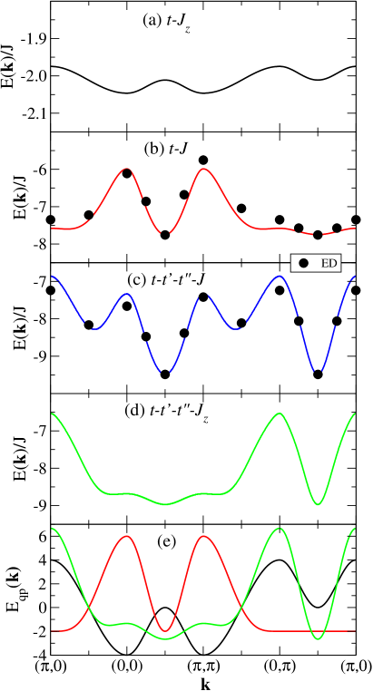
Figure 2: (color online) Quasiparticle energy $E({\bf k})$ along several cuts in the Brillouin zone for various one-band models. In all cases $J/t=0.3$ while $t^{\prime}=t^{\prime\prime}=0$ in (a),(b), and $t^{\prime}/t=-0.3,t^{\prime\prime}/t=0.2$ in (c),(d). Lines show the results of the variational calculation with the spin fluctuations frozen in (a) and (d), or allowed only near the hole in (b) and (c). Symbols in (b) and (c) are the corresponding ED results for a 32-site cluster Leung95 ; Leung97 . (e) Dispersion $E_{qp}({\bf k)}$ of Eq. (11) for $E_{0}=0$ and $t_{2}=-1,t_{3}=0$ (black); $t_{2}=1,t_{3}=0.5$ (red); $t_{2}=-1;t_{3}=2/3$ (green).

The quality of our variational approximation is illustrated in panels (b) and (c). Its results (thick lines) are in fair agreement with those of exact diagonalization (ED) for a 32-site cluster, which includes all spin fluctuations Leung95 ; Leung97 . Results in panel (c) agree well with those measured experimentally Leung97 ; Damascelli . Our bandwidths are somewhat different; some of this may be due to finite-size effects, as the ED bandwidth varies with cluster size Bayo . This also suggests that more configurations need to be included before full convergence is reached by our variational method (these would increase the bandwidth in panel (b) and decrease it in panel (c), see below). This is supported by Ref. MonaHolger , where full convergence for the $t$-$J_{z}$ model was reached when configurations with up to 5 magnons were included. Nevertheless, the agreement is sufficiently good to conclude that the essential aspects of the quasiparticle physics are captured by the three-magnon variational calculation, and to confirm that it suffices to include spin fluctuations only near the hole.

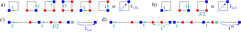
Figure 3: (color online) (a) Shortest Trugman loop that generates a $t_{2,\rm TL}$ contribution. A much smaller $t_{3,\rm TL}$ is also generated, see Ref. MonaHolger ; Generation of (b) $t_{2,\rm sf}$ and (c) $t_{3,\rm sf}$ terms due to spin-fluctuations; (d) Process that renormalizes $t^{\prime\prime}$. The square shows the location of the hole, while the circles show magnons (wrongly oriented spins). The remaining spins are in their Néel order orientation and are not shown explicitly. The short thick arrows indicate the next step in the process, while the thin arrows in the final sketch show the effective quasiparticle hopping generated by those processes.

These results clearly demonstrate that both spin fluctuations and longer-range hopping are needed to achieve the correct quasiparticle dispersion shown in panel (c), with deep, nearly isotropic minima at $({\pi\over 2},{\pi\over 2})$. Absence of longer-range hopping leads to a rather flat dispersion along $(0,\pi)-(\pi,0)$, see panel (b); this fact has long been known Leung95 . In panel (d), we show that if the longer range hopping is included but spin fluctuations are absent, the dispersion is rather flat along the $(0,0)-(\pi,\pi)$ direction. We are not aware of previous studies of this case.

Although $E({\bf k})$ looks very different in the four cases, it turns out that all can be understood in a simple, unified picture. The key insight is that the quasiparticle lives on one magnetic sublattice, because of spin conservation. As a result, its generic dispersion must be of the form:

$$E_{qp}({\bf k})=E_{0}+4t_{2}\cos k_{x}\cos k_{y}+2t_{3}(\cos 2k_{x}+\cos 2k_{y})$$ (11)

i.e. like the bare hole dispersion $\epsilon({\bf k})$ of Eq. (9), but with renormalized 2^nd and 3^rd nn hoppings $t^{\prime}\rightarrow t_{2};t^{\prime\prime}\rightarrow t_{3}$. There cannot be any effective nn hopping of the quasiparticle because this would move it to the other sublattice; this cannot happen without changing the magnetic background, so $t_{1}=0$. Longer range hoppings that keep the quasiparticle on the same sublattice may also be generated dynamically, but their magnitude is expected to be small compared to $t_{2},t_{3}$, hence Eq. (11). Thus, understanding the shape of the quasiparticle dispersion requires understanding the values of $t_{2}$ and $t_{3}$.

We begin the analysis with the $t$-$J_{z}$ model. Its quasiparticle is extremely heavy, as shown in panel (a). Note that the vertical scale is an order of magnitude smaller than for the other panels. The reason is that every time the hole hops, it moves to the other magnetic sublattice and it must either create or remove a magnon, to conserve the total spin. As the hole moves away from its original location, it leaves behind a string of magnons whose energy increases roughly linearly with its length. This could be expected to result in confinement (infinite effective mass), but in fact the quasiparticle acquires a finite dispersion by executing Trugman loops (TL) Trugman , the shortest of which is sketched in Fig. 3(a). By going nearly twice along a closed loop, creating a string of magnons during the first round and removing them during the second round, the hole ends up at a new location on the same magnetic sublattice. Only 2^nd and 3^rd nn hopping terms can be generated through TL irrespective of their length, and $|t_{3,\rm TL}|\ll|t_{2,\rm TL}|\ll J$ if $t/J\sim 3$ MonaHolger . Indeed, setting $t_{2}<0,t_{3}\rightarrow 0$ in $E_{qp}({\bf k})$ of Eq. (11) leads to the black curve in Fig. 2(e) c1 , which has the same shape as that of panel (a) (the bandwidth is proportional to $|t_{2,\rm TL}|$). This dispersion is wrong not just quantitatively but also qualitatively, with $({\pi\over 2},{\pi\over 2})$ as a saddle point instead of the ground state. Clearly, ignoring both longer range hopping and spin fluctuations changes completely the dynamics of the quasiparticle.

When the spin fluctuations are turned on in the $t$-$J$ model, they act on a time scale $\tau_{\rm sf}\sim 1/J$ much faster than the slow dynamics due to TL, $\tau_{\rm TL}\sim 1/|t_{2,\rm TL}|$. The main contributions to $t_{2}$ and $t_{3}$ now come from processes like those sketched in Fig. 3(b) and (c), where spin fluctuations remove pairs of magnons created by nn hopping of the hole, leading to $t_{2,{\rm sf}}\gg|t_{2,\rm TL}|,t_{3,\rm sf}\gg|t_{3,\rm TL}|$. Moreover, we expect $t_{2,\rm sf}=2t_{3,\rm sf}$ because these effective hoppings are generated by similar processes but there are twice as many leading to 2^nd compared to 3^rd nn hopping, as the hole can move on either side of a plaquette.

Indeed, the $t$-$J$ dispersion of panel (b) has a shape similar to that of $E_{qp}({\bf k})$ with $t_{2}=2t_{3}$, shown as a red curve in Fig. 2(e) c2 . Because $E_{qp}(k,\pi-k)=E_{0}-2t_{2}+(4t_{3}-2t_{2})\cos 2k$, it has a perfectly flat dispersion along $(0,\pi)-(\pi,0)$ for $t_{2}=2t_{3}$. The dispersion in panel (b) is not perfectly flat along this cut, so in reality $t_{2}\approx 2t_{3}$. The small correction from the factor of 2 is likely due to higher order processes, as well as contributions from TL (which remain active). Ignoring it, we find the corresponding bandwidth $E_{qp}(0,0)-E_{qp}({\pi\over 2},{\pi\over 2})=4t_{2}+8t_{3}=8t_{2}$, suggesting that the effective hoppings generated with spin fluctuations are of the order $t_{2,\rm sf}\approx 2t_{3,\rm sf}\approx J/4$.

Next, we consider what happens if instead of (local) spin fluctuations, we turn on longer-range hopping. Unlike in the $t$-$J_{z}$ model, the quasiparticle of the $t$-$t^{\prime}$-$t^{\prime\prime}$-$J_{z}$ model should be light because the longer range hoppings $t^{\prime},t^{\prime\prime}$ allow the hole to move freely on its magnetic sublattice. It can therefore efficiently remove magnons created through its nn hopping, without having to complete the time-consuming Trugman loops. The presence of the magnon cloud renormalizes these bare hoppings to smaller values, as is typical for polaron physics. Figure 3(d) shows one such process that renormalizes $t^{\prime\prime}\rightarrow t^{\prime\prime*}$. Similar processes (not shown) renormalize $t^{\prime}\rightarrow t^{\prime*}$ so both hopping integrals should be renormalized by comparable factors. As a result, we expect a dispersion like $E_{qp}({\bf k})$ but now with $t_{2}/t_{3}=t^{\prime*}/t^{\prime\prime*}\approx t^{\prime}/t^{\prime\prime}$, if we ignore the small TL contributions. This indeed agrees with the result in panel (d), as shown by its comparison with the green curve in Fig. 2(e) where $E_{qp}({\bf k})$ is plotted for $t_{2}/t_{3}=t^{\prime}/t^{\prime\prime}=-1.5$. For $t_{2}=-2t_{3}$, $E_{qp}({\bf k})$ would be perfectly flat along $(0,0)-(\pi,\pi)$. Thus, the change in the relative sign explains why now the dispersion is nearly flat along $(0,0)-(\pi,\pi)$ and maximal along $(0,\pi)-(\pi,0)$, in contrast to the previous case. However, while $t_{2,\rm sf}/t_{3,\rm sf}\approx$ 2 is always expected for the $t$-$J$ model so its dispersion must have a shape like in Fig. 2(b), in the $t$-$t^{\prime}$-${}^{\prime}t^{\prime\prime}$-$J_{z}$ model the ratio $t^{\prime*}/t^{\prime\prime*}$ mirrors the ratio $t^{\prime}/t^{\prime\prime}$. If this had a very different value than $\approx-2$, the quasiparticle dispersion would change accordingly.

These results allow us to understand the dispersion of the $t$-$t^{\prime}$-$t^{\prime\prime}$-$J$ quasiparticle. This must have contributions from both the spin fluctuations and the renormalized longer range hoppings, plus much smaller TL terms, because the processes giving rise to them are now all active. Indeed, the curve in panel (c) of Fig. 2 is roughly equal to the sum of those in panels (b) and (d). The isotropic minimum at $\left({\pi\over 2},{\pi\over 2}\right)$ is thus an accident, since the dispersion along $(0,0)-(\pi,\pi)$ is controlled by spin fluctuations, and that along $(0,\pi)-(\pi,0)$ is due to the renormalized longer range hoppings. More precisely, because $t_{2,\rm sf}\approx 2t_{3,\rm sf}$, the contributions coming from spin fluctuation interfere destructively for momenta along $(0,\pi)-(\pi,0)$ so dispersion here is controlled by the renormalized $t^{\prime*}\approx-1.5t^{\prime\prime*}$, and viceversa. If $t_{2,\rm sf}\approx|t^{\prime*}|$ (which happens to hold because $J\sim|t^{\prime}|$), the sum gives nearly isotropic dispersion near $\left({\pi\over 2},{\pi\over 2}\right)$. If we change parameters significantly, the dispersion becomes anisotropic (not shown).

Before moving on to contrast this behavior with that of the quasiparticle of the three-band model, we briefly discuss the effect of the three-site term of Eq. (5). The variational results for the four models are shown in Fig. 4. Where direct comparisons can be made, they are again in good quantitative agreement with other work where this term has been included, such as in Ref. Bala . Its inclusion has a qualitative effect only for the $t$-$J_{z}$ model, where the shape of the dispersion is changed in its presence. This is not very surprising because, as discussed, the Trugman loops which control behavior in that case are very slow processes, and their effect can easily be undone by terms that allow the hole to move more effectively. The three-site term is such a term and its presence increases the bandwidth not just for the $t$-$J_{z}$ model, but for all cases. For the other three models, however, the inclusion of this term changes the dispersion only quantitatively: the bandwidth is increased but the overall shape is not affected much. The biggest change is along $(0,0)-(\pi,\pi)$, as expected because the three-site term generates effective 2nd and 3rd nn hoppings with the same sign and a 2/1 ratio, i.e. similar to $t_{2,sf}$ and $t_{3,df}$. As a result, its presence mimics (and boosts) the effect of the local spin fluctuations.

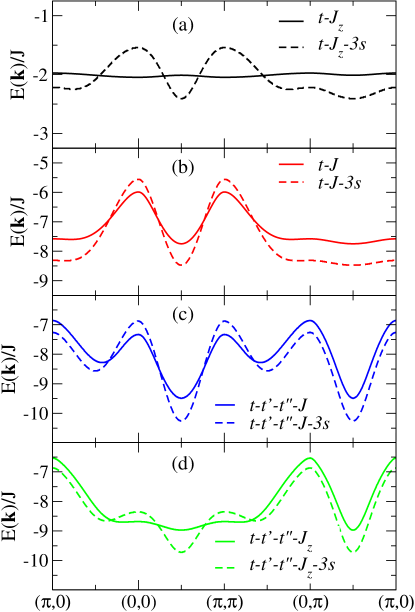
Figure 4: (color online) Quasiparticle dispersion when the three-site term of Eq. (5) is included in the one-band Hamiltonians (dashed lines). For comparison, the dispersions without this term are also show (full lines from Fig. 2)

It is interesting to note that if we allow this term to be large enough, we could obtain a dispersion with the correct shape even in the absence of spin fluctuations. However, the scale of this term is set by $J$, it is not a free parameter. As a result, we conclude that with its proper $J$ energy scale, this terms does not change qualitatively the behavior of the quasiparticle of the one-band model (apart from the $t$-$J_{z}$ case), although its inclusion may, in principle, allow for better fits of the experimental data.

IV.2 Three-band model

Results for the simplified three-band model with the spin-fluctuations frozen off were discussed in Ref. Hadi . To keep this work self-contained, we show in Fig. 5 the most relevant data for the issue of interest, namely the quasiparticle dispersion $E({\bf k})$ obtained in a variational calculation with the maximum number of magnons $n_{m}=0-3$. These results already suffice to illustrate the qualitative difference between the quasiparticle dynamics in the one-band and the three-band models.

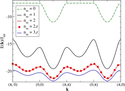
Figure 5: (color online) $E({\bf k})$ along several cuts in the Brillouin zone for the three-band model. The results are for the variational calculation with the spin-fluctuations turned off and configurations with up to $n_{m}$ magnons allowed. The “restricted” calculations labelled $n_{2,r},n_{3,r}$ imposed the additional constraint that the magnons are on adjacent sites. While the bandwidth is strongly renormalized with increasing $n_{m}$, the nearly isotropic dispersion around the ground-state at $({\pi\over 2},{\pi\over 2})$ is a consistent feature. See text for more details.

The $n_{m}=0$ curve plots the dispersion if no magnons are allowed, i.e. not only the spin fluctuations of the AFM background but also spin-flip processes due to $J_{pd}$ and $T_{\rm swap}$ are turned off. It is important to emphasize that the resulting dispersion does contain a very important contribution from the terms in $T_{\rm swap}$ describing hopping of the hole past Cu spins with the same spin projection, so that the spin-swap leaves the spins unchanged.

In fact, it is the interference between these terms with those of $T_{pp}$ that leads to this interesting bare dispersion, which already has deep, nearly-isotropic minima near $({\pi\over 2},{\pi\over 2})$. If we set $t_{sw}=0$, the bare dispersion due to only $T_{pp}$ has the ground-state at $(\pi,\pi)$, whereas if $T_{pp}=0$, the dispersion due to the allowed terms in $T_{\rm swap}$ is perfectly flat because the hole is then trapped near a like Cu spin. However, as long as $t_{pp}\sim t_{sw}$, the isotropic minimum emerges at $({\pi\over 2},{\pi\over 2})$. In this context, it is useful to note that in many numerical studies of the Emery model, $t_{pp}$ was set to zero simply for convenience. Our results suggest that this choice changes the quasiparticle dynamics qualitatively, and is therefore unjustified.

The bare hole dispersion in the three-band model thus already mimics this key aspect of the correct quasiparticle dispersion, unlike in the one-band model. Allowing the quasiparticle cloud to emerge by allowing the hole to create and absorb magnons in its vicinity, through spin-flip processes controlled by $J_{pd}$ and $T_{\rm swap}$, further renormalizes the bandwidth (a typical polaronic effect) without affecting the existence of the isotropic dispersion near $({\pi\over 2},{\pi\over 2})$. This magnon cloud is very important, however, to stabilize the low-energy quasiparticle, as demonstrated by the significant lowering of the total energy. In particular, at least one magnon must be present in order for a ZRS-like object to be able to form, and indeed the $n_{m}=1$ curve is pushed down by $\sim 10J_{dd}$ compared to the bare dispersion. We further analyze the relevance of the ZRS solution below.

The small difference between the $n_{m}=2$ and $n_{m}=2,r$ results proves that magnons indeed sit on adjacent sites in the cloud. (The latter solution imposes this constraint explicitly, whereas the former allows the magnons to be at any distance from each other. In both cases, the hole can be arbitrarily far from the magnons, although, as expected, configurations where the hole is close to the last emitted magnon have the highest weight in the quasiparticle eigenstates.) At higher energies, however, these two solutions are qualitatively different. The former contains the expected quasiparticle+one-magnon continuum starting at $E_{1,gs}+2J_{dd}$, where $E_{1,gs}$ is the ground-state energy of the quasiparticle with $n_{m}=1$, and $2J_{dd}$ is the energy cost to create a magnon far from it. Their sum is the energy above which higher-energy (excited) states must appear in the spectrum, describing the quasiparticle plus one magnon not bound to its cloud. The presence of this continuum guarantees that in the fully converged limit, the quasiparticle bandwidth cannot be wider than $2J_{dd}$, since the quasiparticle band is always “flattened out” below this continuum (another typical polaronic behavior). For both $n_{2,r}$ and $n_{3,r}$ calculations, the quasiparticle is already heavy enough that its dispersion fits below the corresponding continuum. This is why enlarging the variational space with configurations needed to describe this feature, with at least one magnon located far from the cloud, does not affect the quasiparticle dispersion much (see Ref. Hadi for more discussion).

The bandwidth of the $n_{m}=3,r$ dispersion is in decent agreement with numerical results for this model, as discussed next, suggesting that this variational calculation is close to fully converged. The fact that the cloud is rather small should not be a surprise. The variational approach explicitly imposes the constraint that there is at most one magnon at a site. As magnons sit on adjacent sites when bound in the quasiparticle cloud, they prefer to occupy a compact area to minimize their exchange energy cost, thus creating a domain in the other Néel state (down-up instead of up-down). The hole prefers to sit on the edge of this domain, because being inside it is equally disadvantageous to being outside, i.e. far from magnons. However, since on the boundary the hole can interact with only one magnon at one time, a large and costly domain is unlikely.

We can now contrast the dynamics of the quasiparticle in the three-band model if the spin fluctuations are frozen out with the corresponding one-band model, namely the $t$-$t^{\prime}$-$t^{\prime\prime}$-$J_{z}$ case. Both have a quasiparticle with a small, few-magnon cloud, and a bandwidth $\approx 2J=2J_{dd}$. The key difference is that the three-band model already shows a dispersion with the correct shape, whereas for the one-band model the dispersion is much too flat along $(0,0)-(\pi,\pi)$. This difference is traced back to the fact that in the one-band model, the bare hole dispersion also suffers from this same problem if $t^{\prime}/t^{\prime\prime}\sim-1.5$, unlike that of the three-band model. As a result, spin fluctuations are necessary to find the correct dispersion in the one-band model, as already shown, but their role in the three-band model should be rather limited.

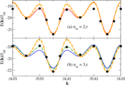
Figure 6: (color online) $E({\bf k})$ along several cuts in the Brillouin zone for the three-band model in the restricted variational approximations with (a) $n_{m}=2$ and (b) $n_{m}=3$. Circles show ED results for $S_{T}={1\over 2}$ from Ref. Bayo for a 32 Cu + 64 O cluster, shifted to have the same ground-state energy. Full lines show the results of Fig. 5, without spin fluctuations. Orange lines with square symbols are the results if spin fluctuations occur near the hole. The dashed green line in panel (b) is the dispersion when spin fluctuations are allowed to locally create/remove a pair of magnons only if no other magnons are present/remain in the system. See text for more details.

To confirm this conjecture, we consider the effect of local spin fluctuations on the dispersion of the three-band model quasiparticle. In Fig. 6, results for the restricted variational approach with $n_{m}=2,r$ and $n_{m}=3,r$ (i.e. up to two or up to three magnons on adjacent sites) are compared to the ED results of Ref. Bayo , shown by the black full circles. Full lines (red and blue, respectively) show the results of Fig. 5, without spin fluctuations. Orange lines with squares show the dispersion with spin fluctuations turned on near the hole. The dashed green line in panel (b) shows an intermediate result when spin fluctuations are allowed to create a pair of magnons only if there is no magnon in the system, and to remove a pair if only two magnons are present (the orange line also includes contributions from processes where spin fluctuations add a pair of magnons when a magnon is already present, and its reversed process).

The effect of spin fluctuations is similar to that found in the one-band models, as expected because the AFM background is modeled identically. They again have very little effect on the $(\pi,0)-(0,\pi)$ dispersion; beside a small shift to lower energies, this bandwidth is only slightly increased, bringing it into better agreement with the ED values for $n_{m}=3$. Like for one-band models, spin fluctuations lead to a more significant increase of the $(0,0)-(\pi,\pi)$ dispersion. For $n_{m}=3$, it changes from being too narrow without spin fluctuations, to too wide in their presence. (The $n_{m}=2$ overestimate of the bandwidth is expected, see discussion in Ref. Hadi ).

The increased energy near $(0,0)=(\pi,\pi)$ may seem problematic but one must remember that in reality, $E({\bf k})$ is flattened below a continuum that appears at $2J_{dd}$ above the ground state. The continuum is absent in this restricted calculation because configurations with a magnon far from the cloud, which give rise to it, are not included. This explains why the overestimated bandwidth is possible. In the presence of the continuum, states that overlap with it hybridize with it and a discrete state (the quasiparticle) is pushed below its edge. This will lower the value at $(0,0)$ and lead to good quantitative agreement everywhere with the ED results. (The keen reader may note that the ED bandwidth is also slightly wider than $2J_{dd}$, but one must remember both the finite size effects of cluster ED, and the existence of a $S_{T}={3\over 2}$ polaron in its spectrum Bayo . Since the total spin ${\hat{\bf S}}_{T}^{2}$ is not a good quantum number in our variational approximation, its quasiparticle probably overlaps somewhat with both the $S_{T}={1\over 2}$ and $S_{T}={3\over 2}$ spin-polarons, so it is not clear which ED states to compare against).

Our results show that spin fluctuations have a similar effect in both models. However, while they are essential for restoring the proper shape of the dispersion in one-band models, they are much less relevant for the three-band model. This is a direct consequence of the different shape of the bare bands, as discussed, but also to having $J\sim|t^{\prime}|$ while $J_{dd}\sim t_{pp}/4$. In the three-band model, the quasiparticle creates and absorbs magnons while moving freely on the O sublattice, on a timescale that is faster than that over which spin fluctuations act, and so their effect is limited. In contrast, in the one-band model, the timescale for free propagation of the hole on the same magnetic sublattice (controlled by $t^{\prime},t^{\prime\prime}$) is comparable with the spin fluctuations’ timescale, and therefore the effect of spin fluctuations is much more significant. They are especially important along $(0,0)-(\pi,\pi)$, where the bare dispersion of one-band models is nearly flat.

V Discussion and summary

In this work, we used a variational method to study and compare the quasiparticle of $t$-$J$ and $t$-$t^{\prime}$-$t^{\prime\prime}$-$J$ one-band models, to that of a (simplified) three-band model that is the intermediary step between the full three-band Emery model and the one-band models.

Our variational method generates the BBGKY hierarchy of equations of motions for a propagator of interest (here, the retarded one-hole propagator), but simplified by setting to zero the generalized propagators related to projections on states that are not within the variational space. Its physical motivation is very simple: if the variational space is properly chosen, i.e. if it contains the configurations with the highest weight contributions to the quasiparticle eigenstates, then the ignored propagators are indeed small because their residue at the $\omega=E({\bf k})$ pole is proportional to their weight (Lehmann representation). Setting them to zero should thus be an accurate approximation. Numerically, the motivation is also clear: because the resulting simplified hierarchy of coupled equations can be solved efficiently, we can quite easily study a quasiparticle (or a few MonaPRL ) on an infinite plane, thus avoiding finite-size effects and getting full information about ${\bf k}$ dependence, not just at a few values. Moreover, by enlarging the variational space and by turning off various terms in the Hamiltonian, both of which lead to changes in the EOM and thus the resulting propagators, one can infer whether the calculation is close to convergence and isolate and understand the effect of various terms, respectively. The ability to efficiently make such comparisons is essential because it allows us to gain intuition about the resulting physics.

Our results show that even though for reasonable values of the parameters, the quasiparticle dispersion $E({\bf k})$ has similar shapes in both models, the underlying quasiparticle dynamics is very different. In the three-band model, the bare dispersion of the hole on the O sublattice, due to $t_{pp}$ and spin-swap hopping $t_{\rm sw}$ past Cu with parallel spins, already has a deep isotropic minimum near $\left({\pi\over 2},{\pi\over 2}\right)$, unlike the bare $\varepsilon({\bf k})$ of the one-band models. When renormalized due to the magnon cloud, it produces a quasiparticle dispersion with the correct shape in the whole Brillouin zone, even in the absence of spin fluctuations. In contrast, for the one-band models the inclusion of spin fluctuations is necessary for the correct dispersion to emerge. This shows that the quasiparticle dynamics is controlled by different physics in the two models, and this is likely to play a role at finite concentrations as well.

Our results thus raise strong doubts on whether the one-band $t$-$t^{\prime}$-$t^{\prime\prime}$-$J$ model truly describes the same physics like the three-band model. We can think of three possible explanations to explain these differences:

(i) The $t$-$t^{\prime}$-$t^{\prime\prime}$-$J$ model is the correct one-band model, but its true parameters have values quite different from the ones used here. Indeed, if the bare $\varepsilon({\bf k})$ dispersion had isotropic minima at $({\pi\over 2},{\pi\over 2})$, and if its renormalized bandwidth would be of the order of $2J$, then spin fluctuations could not change it much, similar to what is observed in the three-band model.

This explanation can be ruled out. An isotropic bare dispersion $\varepsilon(k,k)\approx\varepsilon(k,\pi-k)$ requires that $|t^{\prime\prime}/t^{\prime}|\gg 1$, which is physically unreasonable.

(ii) The $t$-$t^{\prime}$-$t^{\prime\prime}$-$J$ model has a different quasiparticle because its underlying assumption, i.e. the existence of the low-energy ZRS, is wrong. This would mean that not only this specific one-band model but any other one obtained through such a projection would be invalid.

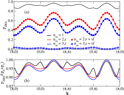
Figure 7: (color online) (a) Overlap $p_{\rm ZRS}$ between the ZRS Bloch state of Eq. (12) and the quasiparticle eigenstate, as obtained in the restricted variational calculations with $n_{m}=1,2,3$, without (full lines) and with (full symbols) local spin fluctuations included. The empty squares and the dashed line show the weight of the ZR triplet. (b) Overlap $p_{\rm ZRS}$ normalized with respect to the probability to have no magnon ($p_{0}$) or to have one magnon near the hole ($p_{1}$), in the quasiparticle eigenstate. See text for more details.

We can test this hypothesis by calculating the overlap between the three-band quasiparticle and a ZRS Bloch state. The latter is defined in the only possible way that is consistent with Néel order:

$$|{\rm ZRS},{\bf k}\rangle={1\over\sqrt{N}}\sum_{i\in{\rm Cu}_{\downarrow}}e^{i{\bf k}\cdot{\bf R}_{i}}{p^{\dagger}_{x^{2}-y^{2},i,\uparrow}-p^{\dagger}_{x^{2}-y^{2},i,\downarrow}S_{i}^{+}\over\sqrt{2}}|{\rm N}\rangle$$ (12)

where

$$p^{\dagger}_{x^{2}-y^{2},i,\sigma}={1\over 2}\left[p^{\dagger}_{i+{{\bf x}\over 2},\sigma}+p^{\dagger}_{i+{{\bf y}\over 2},\sigma}-p^{\dagger}_{i-{{\bf x}\over 2},\sigma}-p^{\dagger}_{i-{{\bf y}\over 2},\sigma}\right]$$

is the linear combination of the $p$ orbitals neighbor to the Cu located at $i$, that has the overall $x^{2}-y^{2}$ symmetry (our choice for the signs of the lobs is shown in Fig. 1). Note that with this definition $|\langle{\rm ZRS},{\bf k}|{\rm ZRS},{\bf k}\rangle|^{2}=1$ for any ${\bf k}$, so there are no normalization problems Zhang .

We define $p_{\rm ZRS}=|\langle qp,{\bf k}|{\rm ZRS},{\bf k}\rangle|^{2}$ as the overlap between the quasiparticle eigenstate of momentum ${\bf k}$ and this ZRS Bloch state. Its value can be calculated from the appropriate residues of the zero- and one-magnon propagators at $\omega=E({\bf k})$, and is shown in Fig. 7(a). We do not plot the $n_{m}=0$ results because a singlet cannot form if the Cu spins cannot flip. (For $n_{m}=0$, there is overlap with the spin-up hole component of $|{\rm ZRS},{\bf k}\rangle$, and we find that $p_{\rm ZRS}$ varies from 0 at $(0,0)$ and $(0,\pi)$ to 0.5 at $({\pi\over 2},{\pi\over 2})$, but the same answer is found for a triplet. Interestingly, this proves that the bare hole dispersion already has eigenstates with the $x^{2}-y^{2}$ symmetry near $({\pi\over 2},{\pi\over 2})$).

For $n_{m}=1$ we find $p_{\rm ZRS}\sim 0.9$ in the entire Brillouin zone. Clearly, in this very small variational space, locking into a ZRS is the best way for the doped hole to lower its energy. However, the value of $p_{\rm ZRS}$ decreases fairly significantly for $n_{m}=2,r$ and $n_{m}=3,r$. First, note that turning the spin fluctuations on or off has almost no effect on $p_{\rm ZRS}$. This is consistent with our conclusion that local spin fluctuations do not influence the nature of the quasiparticle in the three-band model: clearly, its wavefunction is not changed in their presence.

The decrease of $p_{\rm ZRS}$ with increasing $n_{m}$ could be due either to increased contributions to the eigenstate from many-magnon configurations (which have no overlap with $|{\rm ZRS},{\bf k}\rangle$), and/or from competing states such as a ZR triplet, and/or singlets or triplets with the hole occupying a linear combination of O orbitals with $s,p_{x}$ or $p_{y}$ instead of $x^{2}-y^{2}$ symmetry. The latter possibility can also be ruled out because overlaps with those Bloch states are found to be small. The largest such contribution is from the ZR triplet state, shown in Fig. 7(a) by the dashed line and open squares for $n_{m}=3,r$ without and with local spin fluctuations, respectively. This overlap is much smaller than with the ZRS singlet.

Another way to confirm this is displayed in Fig. 7(b), where we compare $p_{\rm ZRS}$ to $p_{0}+p_{1}$, where $p_{0}$ is the probability to find the hole without any magnons, and $p_{1}$ is the probability to find one magnon adjacent to the hole, in the quasiparticle eigenstate. Note that $p_{0}+p_{1}<1$ even for the one-magnon variational approximation because the hole can also be located away from the magnon. As $n_{m}$ increases, $p_{0}+p_{1}$ decreases even more as configurations with two or more magnons now also contribute to the normalization. These configurations with two or more magnons, and those with one magnon not adjacent to the hole, have no overlap with $|{\rm ZRS},{\bf k}\rangle$, explaining the decrease in the magnitude of $p_{\rm ZRS}$. However, the ratio $p_{\rm ZRS}/(p_{0}+p_{1})>0.9$ in the whole Brillouin zone, confirming that this part of the wavefunction has a predominant ZRS-like nature. This is certainly the case near the $({\pi\over 2},{\pi\over 2})$ point, where the overlap is converged to 1. Interestingly, at the antinodal points this ratio decreases with increasing $n_{m}$, and here the overlap with the ZR triplet is largest, see Fig. 7(a), suggesting that a ZRS description is less accurate in this region.

Thus, the zero- and one- (adjacent) magnon parts of the wavefunction have significant overlap with the ZRS Bloch state. However, $p_{\rm ZRS}\sim 0.5$ is a rather small value, and it is not clear whether the dressing with more magnons is consistent with this ZRS picture or not. It is possible that the two- and three-magnon components of the wavefunction have significant overlap with a ZRS+one magnon and ZRS+two magnon configurations, but they could also have quite different nature. It is not clear to us how to verify which is the actual situation.

If these two- and three-magnon components have significant non-ZRS character, however that is defined in this case, then clearly the difference observed in the results from one- and three-band models would be likely due to this non-ZRS nature.

If, on the other hand, one takes these results to support the idea that a low-energy projection onto ZRS states is valid, then this is not the origin of the discrepancy in the quasiparticle behavior. In this case, it must follow that:

(iii) The $t$-$t^{\prime}$-$t^{\prime\prime}$-$J$ is not the correct one-band model because there are additional important terms generated by the projection onto the ZRS states, like those discussed in Ref. ALigia or the three-site terms, which it neglects.

If (iii) is indeed the explanation for the different behavior of the quasiparticles of the one- and three-band models, then in our opinion this implies that the strategy of using one-band models to study cuprates is unlikely to succeed. The main reason for this strategy, as mentioned, is to make the Hilbert space as small as possible for computational convenience. This, however, is only useful if the Hamiltonian is also fairly simple.

In principle one could test additional terms that could be included in one-band models by using methods like ours, to figure out which insure that the resulting behavior mirrors that of the three-band model. Even if this enterprise was successful and the “fix” was relatively simple, i.e. only a few additional terms and corresponding parameters are necessary, it is important to emphasize that this improved one-band model would still not describe correctly cuprates at finite doping. Additional terms must be included to correctly account for the effective interactions between quasiparticles in one-band models, as we demonstrated in Ref. Mirko .

From a technical point of view, their origin is simple to understand. Even for the simplified three-band model, the presence of additional holes leads to additional terms in the Hamiltonian BayoPRB , because the intermediary states are different and this affects the projection onto states with no-double occupancy on Cu. This is going to become even more of an issue if a subsequent projection onto ZRS-like states has to be performed, and may well result in an unmanageably complex Hamiltonian.

This is why we believe that the (simplified) three-band model is a safer option to pursue. Its computational complexity is not that much worse than for one-band models, whereas the Hamiltonian is certainly simpler. In fact, our demonstration here that there is no need to accurately capture the spin fluctuations of the AFM background in order to gain a reasonable understanding of the quasiparticle behavior, makes its study significantly simpler. In particular, it allowed us to study one hole on an infinite layer very simply and efficiently. Generalizations to few holes MonaPRL and to finite concentrations could also turn out to be easier to carry out than the effort of finding the correct form for a one-band Hamiltonian.

Of course, there is no guarantee that the (simplified) three-band model captures all physics needed to explain cuprates, either. It is possible that important aspects of the Emery model were lost through the projection onto spin degrees of freedom at the Cu sites (this, however, would affect the one-band models just as much). Even the Emery model itself may not be general enough; for instance, a generalization to a 5-band model including non-ligand O $2p$ orbitals might be needed, as suggested recently in Ref. Hirsch . We note that such a generalization can be easily handled by our method (provided that one can still project onto spin degrees of freedom at the Cu sites), as showed in Ref. Hadi where we found that these states do not change the quasiparticle dispersion much, although they do have an effect on its wavefunction.

While careful investigation of such scenarios is left as future work, one clear lesson from this study is that obtaining the correct dispersion for the quasiparticle of an effective model is not sufficient to validate that model. The dispersion can have the correct shape for the wrong reasons, as we showed to be the case for the $t$-$t^{\prime}$-$t^{\prime\prime}$-$J$ model, where it is due to the interplay between the effects of the longer-range hopping and spin-fluctuations. The same dispersion is obtained for the simplified three-band model, however in this case the spin-fluctuations play essentially no role, so the underlying physics is very different. This difference is very likely to manifest itself in other properties, therefore these models are not equivalent despite the similar dispersion of their quasiparticles.

- (1) J. G. Bednorz and K. A. Muller, Z. Phys. B 64, 189 (1986).
- (2) P.A. Lee, N. Nagaosa and X.-G. Wen, Rev. Mod. Phys. 78, 17 (2006); M. Ogata and H. Fukuyama, Rep. Prog. Phys. 71, 036501 (2008); P. A. Lee, Rep. Prog. Phys. 71, 012501 (2008); P. Phillips, Rev. Mod. Phys. 82, 1719 (2010).
- (3) see, for instance, B. I. Shraiman and E. D. Siggia, Phys. Rev. Lett. 60, 740 (1988); C. L. Kane, P. A. Lee, and N. Read, Phys. Rev. B 39, 6880 (1989); S. Sachdev, Phys. Rev. B 39, 12232 (1989); F. Marsiglio, A. E. Ruckenstein, S. Schmitt-Rink, and C. M. Varma, Phys. Rev. B 43, 10882 (1991); A. V. Chubukov and D. K. Morr, Phys. Rev. B 57, 5298 (1998).
- (4) H. Zaanen, G. A. Sawatzky, and J. W. Allen, Phys. Rev. Lett. 55, 418 (1985).
- (5) V. J. Emery, Phys. Rev. Lett. 58, 2794 (1987).
- (6) F.C. Zhang and T.M. Rice, Phys. Rev. B 37, 3759 (1988).
- (7) H. Eskes and G.A. Sawatzky, Phys. Rev. Lett. 61, 1415 (1988).
- (8) B. O. Wells, et al, Phys. Rev. Lett. 74, 964 (1995).
- (9) P. W. Leung and R. J. Gooding, Phys. Rev. B 52, R15711 (1995); ibid Phys. Rev. B 54, 711 (1996).
- (10) A. Damascelli, Z. Hussain, and Z-X. Shen, Rev. Mod. Phys. 75, 473 (2003).
- (11) P. W. Leung, B. O. Wells, and R. J. Gooding, Phys. Rev. B 56, 6320 (1997).
- (12) E. Pavarini, I. Dasgupta, T. Saha-Dasgupta, O. Jepsen, and O. K. Andersen, Phys. Rev. Lett. 87, 047003 (2001); O.K. Andersen, A. I. Liechtenstein, O. Jepsen, and F. Paulsen, J. Phys. Chem. Solids, 56 1573 (1995).
- (13) H. Eskes and G. A. Sawatzky, Phys. Rev. B 44, 9656 (1991).
- (14) K. A. Chao, J. Spalek and A. M. Olés, J. Phys. C: Solid State Phys. 10, L271 (1977); K. A. Chao, J. Spalek, and A. M. Oleś, Phys. Rev. B 18, 3453 (1978); M. Ogata, and H. Shiba, J. Phys. Soc. Jpn. 57 3074 (1988).
- (15) Double occupancy is forbidden on Cu so here doping holes residing on O interact with spins located on Cu.
- (16) H. Ebrahimnejad, G. A. Sawatzky, and M. Berciu, Nature Phys. 10, 951 (2014).
- (17) V. J. Emery and G. Reiter, Phys. Rev. B 38, 4547 (1988); E. Dagotto, A. Moreo, R. Joynt, S. Bacci, and E. Gagliano, Phys. Rev. B 41, 2585(R) (1990); E. Dagotto, R. Joynt, A. Moreo, S. Bacci, and E. Gagliano, Phys. Rev. B 41, 9049 (1990); V. Elser, D. A. Huse, B. I. Shraiman, and E. D. Siggia, Phys. Rev. B 41, 6715 (1990); M. Boninsegni, and E. Manousakis, Phys. Rev. B 43, 10353 (1991); R.T. Scalettar, D.J. Scalapino, R.L. Sugar, S.R. White, Phys. Rev. B 44, 770 (1991); G. Dopf, J. Wagner, P. Dieterich, A. Muramatsu, W. Hanke, Phys. Rev. Lett. 68, 2082 (1992); G. Dopf, A. Muramatsu, W. Hanke, Phys. Rev. Lett. 68, 353 (1992); D. Poilblanc, H. J. Schulz, and T. Ziman, Phys. Rev. B 46, 6435 (1992); T. Giamarchi and C. Lhuillier, Phys. Rev. B 47, 2775 (1993); T. Hotta, J. Phys. Soc. Jpn. 63, 4126 (1994); E. Dagotto, A. Nazarenko and M. Boninsegni, Phys. Rev. Lett. 73, 728 (1994). K. Kuroki, H. Aoki, Phys. Rev. Lett. 76, 4400 (1996); T. Takimoto, T. Moriya, J. Phys. Soc. Jpn. 67, 3570 (1998); S. Koikegami, K. Yamada, J. Phys. Soc. Jpn. 69, 768 (2000); T. Yanagisawa, S. Koike, K. Yamaji, Phys. Rev. B 64, 184509 (2001); P.R.C. Kent, T. Saha-Dasgupta, O. Jepsen, O.K. Andersen, A. Macridin, T.A. Maier, M. Jarrell, T.C. Schulthess, Phys. Rev. B 78, 035132 (2008); C. Weber, K. Haule, G. Kotliar, Phys. Rev. B 78, 134519 (2008); L. de Medici, X. Wang, M. Capone, A.J. Millis, Phys. Rev. B 80, 054501 (2009); X. Wang, L. de’Medici, A.J. Millis, Phys. Rev. B 81, 094522 (2010); A. Avella, F. Mancini, F. P. Mancini, and E. Plekhanov Eur. Phys. J. B 86, 265 (2013);
- (18) Of course, long range AFM order is forbidden in a 2D layer by the Mermin-Wagner theorem, see N. D. Mermin and H. Wagner, Phys. Rev. Lett. 17, 1133 (1966). However, in the real material there is weak coupling between CuO2 layers, sufficient to stabilize the long range AFM order.
- (19) M. S. Hybertsen, E. B. Stechel, M. Schluter, and D. R. Jennison, Phys. Rev. B 41, 11068 (1990).
- (20) see T. Tohyama and S. Maekawa, Supercond. Sci. Technol. 13 R17 (2000) and references therein.
- (21) S. Trugman, Phys. Rev. B 41, 892 (1990); R. Eder and K. W. Becker, Z. Phys. B 78, 219 (1990); R. J. Gooding, K. J. E. Vos, and P. V. Leung, Phys. Rev. B 50, 12866 (1994); G. C. Psaltakis, Phys. Rev. B 45, 539 (1992); G. C. Psaltakis and N. Papanicolaou, Phys. Rev. B 48, 456 (1993).
- (22) A. A. Aligia, M. E. Simon and C. D. Batista, Phys. Rev. B 49, 13061 (1994); F. Lema and A. A. Aligia, Phys. Rev. B 55, 14092 (1997).
- (23) B. Lau, M. Berciu, and G. A. Sawatzky, Phys. Rev. Lett. 106, 036401 (2011).
- (24) J. Zaanen and A. M. Olés, Phys. Rev. B 37, 9423 (1988); D. M. Frenkel, R. J. Gooding, B. I. Shraiman, and E. D. Siggia, Phys. Rev. B 41, 350 (1990); J. L. Shen and C. S. Ting, Phys. Rev. B 41, 1969 (1990); H.-Q. Ding, G. H. Lang, and W. A. Goddard, III, Phys. Rev. B 46, 14317(R) (1992); Y. Petrov and T. Egami, Phys. Rev. B 58, 9485 (1998).
- (25) J. D. Reger and A. P. Young, Phys. Rev. B 37, 5978 (1988); E. Manousakis, Rev. Mod. Phys. 63, 1 (1991); H. G. Evertz, G. Lana, and M. Marcu, Phys. Rev. Lett. 70, 875 (1993); A. W. Sandvik, Phys. Rev. B 59, R14157 (1999); W. M. C. Foulkes, L. Mitas, R. J. Needs, and G. Rajagopal, Rev. Mod. Phys. 73, 33 (2001); F. Mezzacapo, N. Schuch, M. Boninsegni, and J. Ignaciocirac, New J. Phys. 11, 083026 (2009).
- (26) M. Berciu and H. Fehske, Phys. Rev. B 84, 165104 (2011).
- (27) S. A. Trugman, Phys. Rev. B 37, 1597 (1988).
- (28) S. Hadi Ebrahimnejad Rahbari, PhD thesis, University of British Columbia (2014).
- (29) In the limit , arises from 6th order perturbation theory, see MonaHolger .
- (30) In the limit , arises from 3rd order perturbation theory.
- (31) J. Bala, Eur. Phys. J. B 16, 495 (2000).
- (32) M. Berciu, Phys. Rev. Lett. 107, 246403 (2011).
- (33) M. Möller, G. A. Sawatzky and M. Berciu, Phys. Rev. Lett. 108, 216403 (2012); ibid, Phys. Rev. B 86, 075128 (2012).
- (34) B. Lau, M. Berciu, and G. A. Sawatzky, Phys. Rev. B 84, 165102 (2011).
- (35) J.E. Hirsch, Phys. Rev. B 90, 184515 (2014).