Collapse for the higher-order nonlinear Schrödinger equation

Abstract

We examine conditions for finite-time collapse of the solutions of the higher-order nonlinear Schrödinger (NLS) equation incorporating third-order dispersion, self-steepening, linear and nonlinear gain and loss, and Raman scattering; this is a system that appears in many physical contexts as a more realistic generalization of the integrable NLS. By using energy arguments, it is found that the collapse dynamics is chiefly controlled by the linear/nonlinear gain/loss strengths. We identify a critical value of the linear gain, separating the possible decay of solutions to the trivial zero-state, from collapse. The numerical simulations, performed for a wide class of initial data, are found to be in very good agreement with the analytical results, and reveal long-time stability properties of localized solutions. The role of the higher-order effects to the transient dynamics is also revealed in these simulations.

1 Introduction

The present paper deals with the dynamical properties of a higher-order nonlinear Schrödinger (NLS) equation, expressed in dimensionless form:

$${{u}_{t}}+\frac{s}{2}\mathrm{i}{{u}_{xx}}-\mathrm{i}|u|^{2}u=\gamma u+\delta|u|^{2}u+\beta u_{xxx}+\mu(|u|^{2}u)_{x}+\left(\nu-\mathrm{i}\sigma_{R}\right)u(|u|^{2})_{x},$$ (1.1)

for all $x\in\mathbb{R}$, and $t\in[0,T]$ for some $T>0$. In Eq. (1.1), $u(x,t)$ is the unknown complex field, subscripts denote partial derivatives, $\gamma$, $\delta$, $\sigma_{R}$ and $\mu,\,\nu$ are real constants, while $s=1$ corresponds to normal group velocity dispersion. We supplement Eq. (1.1) with the periodic boundary conditions for $u$ and its spatial derivatives up to the second order:

$$u(x+2L,t)=u(x,t),\;\;\mbox{and}\;\;\;\frac{\partial^{j}u}{\partial x^{j}}(x+2L,t)=\frac{\partial^{j}u}{\partial x^{j}}(x,t),\;\;j=1,2,\ \quad\forall\,x\in{\mathbb{R}},\;\;\forall\,t\in[0,T],$$ (1.2)

where $L>0$ is given, and with the initial condition

$$u(x,0)=u_{0}(x),\quad\forall\,x\in{\mathbb{R}},$$ (1.3)

also satisfying the periodicity conditions (1.2). Note that the boundary conditions (1.2) will be incorporated in the Sobolev spaces of periodic functions, that will be used for the analysis of the problem (1.1)-(1.3). Their definition will be recalled and discussed below.

Equation (1.1) finds important applications in distinct physical and mathematical contexts, with the most prominent being that of nonlinear optics. Indeed, such models have been used to describe ultrashort pulse propagation in nonlinear optical fibers in the framework of the slowly-varying envelope approximation [1, 2, 3] (see also reviews [4, 5] and references therein for recent work in few-cycle pulse propagation). In such a case, $t$ and $x$ in Eq. (1.1) play, respectively, the role of the propagation distance along the optical fiber and the retarded time (in a reference frame moving with the group velocity), while $u(x,t)$ accounts for the (complex) electric field envelope. The propagation of optical pulses (of temporal width comparable to the wavelength) is accompanied by effects, such as higher-order (and, in particular, third-order) linear dispersion (characterized by the coefficient $\beta$), as well as nonlinear dispersion (characterized by the coefficient $\mu$). The latter is known as “self-steepening” term, due to its effect on the pulse envelope. These conservative higher-order terms (including the one of strength $\nu$) are naturally important not only in optics, but also in the contexts of nonlinear metamaterials [6, 7, 8] and water waves [9, 10, 11]. All the above effects, which are not incorporated in the standard NLS equation ($\gamma=\delta=\beta=\mu=\nu=\sigma_{R}=0$), become important in the physically relevant case of ultrashort pulses.

On the other hand, and in the same nonlinear optics context, for relatively long propagation distances, dissipative effects, such as linear loss ($\gamma<0$) [or gain ($\gamma>0$)], as well as stimulated Raman scattering (of strength $\sigma_{R}>0$), are also included [1, 2, 3]. At the same time, it is also relevant to include the nonlinear gain ($\delta>0$) [or loss ($\delta<0$)] to counterbalance the effects from the linear loss/gain mechanisms [12]. For relevant physical settings, the role of such terms is to contribute to the possible stabilization of solitons. Notice that such solutions exist in the standard NLS equation, which possesses solitons of two different types: bright solitons (for $s=-1$) that decay to zero at infinity, and dark solitons (for $s=+1$) that have the form of density dips on top of a continuous-wave (cw) background accompanied by a phase jump at the density minimum. Below we focus on the latter case of normal dispersion ($s=+1$), for which the linear/nonlinear dissipative effects usually lead to the decay of the cw background; this way, the composite object, composed by the background and the soliton, is destroyed.

Dark solitons were first predicted to occur as early as in the early 70’s [13, 14], and since then have been studied extensively, both in theory and in experiments, mainly in nonlinear optics [15] and Bose–Einstein condensation [16, 17, 18]. Concerning the higher-order NLS (1.1), in Ref. [19] it was shown, via a newly developed perturbation theory [20], that dark and grey solitons can exist and feature a stable evolution –at least for certain parameter regimes and time intervals, within the validity of the perturbation theory. However, their long-time dynamics are under question. The results of Ref. [19] suggest that these dynamics, and different scenarios corresponding to various parameter regimes, can be very rich.

The structure of the presentation and main findings of the present work are as follows. In Sec. 2, we explore the finite-time collapse for the solutions of Eqs. (1.1)–(1.3). Our analysis is motivated from the results and questions posed on the dynamics of the soliton background discussed in Ref. [19]. The discussion therein, shows that there can be a finite-time for which the background exhibits blow-up. Also in Section 2.1, based on energy arguments carried out on a spatially averaged $L^{2}$-energy functional, we identify that the collapse behavior of the considered $L^{2}$-functional is chiefly characterized by the gain/loss parameters $\gamma$ and $\delta$. Regimes of collapse and decay of solutions are defined by $\gamma,\delta>0$ and $\gamma,\delta<0$. However, for $\gamma<0,\,\delta>0$, we obtain the existence of a critical value on the linear gain. This critical value, say $\gamma^{*}$, is separating finite-time collapse from the decay of solutions. An important conclusion regarding the regimes $\gamma,\delta>0$ and $\gamma,\delta<0$ is related to the fate of localized solutions, with an initial profile resembling that of bright and dark solitons: referring to their long-time stability, such wave forms are unstable, and they may survive only for relevant short times.

The above picture on the asymptotic behavior is verified completely by the results of the numerical simulations presented in Section 3. We examine the evolution for three distinct types of initial conditions, including decaying and non-decaying data. In the case of cw initial conditions, we observe that the analytical upper bound is not only fulfilled, but also saturated by the analytical blow-up times. Furthermore, the numerical collapse time is independent of the strengths of the rest of the dissipative/conservative higher-order terms. The observed saturation is completely justified by the fact that the timescales for collapse of the background, and the analytical upper bound for the collapse of the $L^{2}$ functional, coincide in the case of the cw initial condition. Also, the evolution of the $L^{2}$-functional is proved to be that of the cw-background. Concerning the critical value $\gamma^{*}$, it is verified numerically that its analytical estimation is very accurate; for $\gamma<\gamma^{*}$ the solution decays and for $\gamma\geq\gamma^{*}$ the solution blows-up in finite-time. In the case of the decaying initial data (which are taken in the form of a $\mathrm{sech}$ function – as reminiscent of a bright soliton of the focusing NLS), we have observed very interesting transient dynamics prior to collapse when $\gamma\geq\gamma*$, or decay when $\gamma<\gamma^{*}$, characterized by a self-similar evolution of the initial pulse for small values of the parameters. As before, the analytical upper bound for the blow-up time is in agreement with the numerical one. However, it is not saturated since the evolution of the $L^{2}$ functional is dominated by the evolution of the amplitude of the localized solution. We have also tested numerically the behavior of the blow-up time with respect to large variations of the strengths of linear and nonlinear parameters $\beta$ and $\sigma_{R}$, and found the following decreasing step function effect: the numerical blow-up time jumps to a smaller numerical value but remains constant within specific regimes of variation for the increasing parameters. The jump is associated with a transition to a different type of transient dynamics prior to collapse or decay.

The numerical results were also found to be in excellent agreement with the analytical ones in the case of the non-decaying initial data –taken here in the form of a $\mathrm{tanh}^{2}$ function, which resembles the intensity profile of a dark soliton of the defocusing NLS, and is compliant with the periodic boundary conditions (1.2). The numerical blow-up time is in agreement with –and is also found to almost saturate to– its analytical upper bound, as in the case of the cw-initial condition, at least for small variations of the parameters, for reasons that will be discussed later in the text. In regimes of larger parameter values, we observe again the decreasing step function effect for the numerical blow-up time associated with a drastic change in the transient dynamics. In the case $\gamma<0,\,\delta>0$, it appears that the condition $\gamma\delta<0$ is not sufficient to define a stabilization regime with nontrivial dynamics or avoiding collapse. It will be shown in a subsequent work [21], that such a stabilization regime associated with emergent dynamics different from collapse or decay, may be defined only when $\gamma>0$, $\delta<0$.

2 Conditions for collapse

2.1 Collapse in finite-time for an $L^{2}$-norm functional

The question of collapse concerns sufficiently smooth (weak) solutions of equation (1.1). The existence of such solutions, is guaranteed by the following local existence result associated with the initial-boundary value problem (1.1)-(1.3). The methods which are used in order to prove such local existence result in the Sobolev spaces of periodic functions $H^{k}_{per}$ [26, 28], are based on the lines of approach of [22]-[25]. The application of these methods to the problem (1.1)-(1.3), although involving lengthy computations, is now considered as standard. Thus, we refrain from showing the details here, and we just state it in:

Theorem 2.1.

Let $u_{0}\in H^{k}_{per}(\Omega)$ for any integer $k\geq 2$, and $\beta,\gamma,\delta,\mu,\nu,\sigma_{R}\in\mathbb{R}.$ Then there exists $T>0$, such that the problem (1.1)-(1.3), has a unique solution

$$u\in C([0,T],H^{k}_{per}(\Omega))\quad\mbox{and}\quad u_{t}\in C([0,T],H^{k-3}_{per}(\Omega)).$$

Moreover, the solution $u\in H^{k}_{per}(\Omega)$ depends continuously on the initial data $u_{0}\in H^{k}_{per}(\Omega)$, i.e., the solution operator

$$\mathcal{S}(t):H^{k}_{per}(\Omega) \mapsto H^{k}_{per}(\Omega),\;\;\;\;t\in[0,T],$$ (2.1)

$$u_{0} \mapsto \mathcal{S}(t)u_{0}=u,$$

is continuous.

Here, $H^{k}_{per}(\Omega)$ denote the Sobolev spaces of $2L$- periodic functions on the fundamental interval $\Omega=[-L,L]$. Let us recall for the shake of completeness their definition:

$$H^{k}_{per}(\Omega) = \{u:\Omega\rightarrow\mathbb{C},\;\;u\;\mbox{and}\;\frac{\partial^{j}u}{\partial x^{j}}\in L^{2}(\Omega),\;\;j=1,2,...,k;$$ (2.2)

$$u(x),\;\;\mbox{and}\;\;\frac{\partial^{j}u}{\partial x^{j}}(x)\;\mbox{for $j=1,2,...,k-1$, are $2L$-periodic}\}.$$

Since our analytical energy arguments for examining collapse require sufficiently smoothness of local-in-time solutions, we shall implement Theorem 2.1 by assuming that $k=3$, at least. As it follows from the definition of the Sobolev spaces (2.2), this assumption means that the initial condition $u_{0}(x)$, $x\in\Omega$, and its spatial (weak) derivatives, at least up to the 2nd-order, are $2L$-periodic. Then, it turns out from Theorem 2.1, that the unique, local-in-time solution $u(x,t)$ of (1.1) satisfies the periodic boundary conditions (1.2) for $t\geq 0$, and is sufficiently (weakly) smooth. Such periodicity and smoothness properties of the local-in-time solutions are sufficient for our purposes (see Theorem 2.2 and Appendix A, below).

Next, we adopt the method of deriving a differential inequality for the functional

$$M(t)=\frac{{{e}^{-2\gamma t}}}{2L}\int_{-L}^{L}|u(x,t)|^{2}dx,$$ (2.3)

and then, showing that its solution diverges in finite-time under appropriate assumptions on its initial value at time $t=0$; see [26, 27, 28, 29, 30] and references therein. Note that the choice of this functional is not arbitrary; in fact, it is a direct consequence of the conservation laws of the NLS model (see Appendix A). For a discrete counterpart of this argument applied in discrete Ginzburg-Landau-type equations, we refer to [31]. For applications of these types of arguments in the study of escape dynamics for Klein-Gordon chains, we refer to [32].

Theorem 2.2.

For $u_{0}\in H^{k}_{per}(\Omega)$, $k\geq 3$, let $\mathcal{S}(t)u_{0}=u\in C([0,T_{\mathrm{max}}),H^{k}_{per}(\Omega))$ be the local- in- time solution of the problem (1.1)-(1.3), with $[0,T_{\mathrm{max}})$ be its maximal interval of existence. Assume that the parameter $\delta>0$ and that the initial condition $u_{0}(x)$ is such that $M(0)>0$. Then, $T_{\mathrm{max}}$ is finite, in the following cases:

$$(i)\;\;\;\;\;\;\;\;\;\;\;{{T}_{\mathrm{max}}}\leq\frac{1}{2\gamma}\log\left[1+\frac{\gamma}{\delta M\left(0\right)}\right],$$ (2.4)

$$\mbox{for}\;\;\gamma\neq 0,\;\;\mbox{and}\;\;\ \gamma>-\delta M\left(0\right).$$ (2.5)

$$(ii)\;\;\;\;\;\;\;\;\;\;\;{{T}_{\mathrm{max}}}\leq\frac{1}{2\delta M\left(0\right)},\;\;\mbox{for}\;\;\gamma=0.$$ (2.6)

Proof: For any $T<T_{\mathrm{max}}$, since $k\geq 3$, due to the continuous embedding $C([0,T],H^{k}_{per}(\Omega))\subset C([0,T],L^{2}(\Omega))$ [26], the solution $\mathcal{S}(t)u_{0}=u\in C([0,T],L^{2}(\Omega))$. Furthermore, it follows from Theorem 2.1, that $u_{t}\in C([0,T],L^{2}(\Omega))$. Then, by differentiating $M(t)$ with respect to time, we find that

$$\frac{dM(t)}{dt}=-\gamma\frac{e^{-2\gamma t}}{L}\int_{-L}^{L}|u|^{2}dx+\frac{e^{-2\gamma t}}{L}\mathrm{Re}\int_{-L}^{L}u_{t}\overline{u}dx.$$ (2.7)

In the second term on the right-hand side of (2.7), we substitute $u_{t}$ by the right-hand side of Eq. (1.1). Then, after some computations (see details in Appendix A), Eq. (2.7) results in:

$$\frac{dM(t)}{dt}=\delta\frac{e^{-2\gamma t}}{L}\int_{-L}^{L}|u|^{4}dx.$$ (2.8)

Next, by the Cauchy-Schwarz inequality, we have

$$\int_{-L}^{L}|u|^{2}dx\leq\sqrt{2L}\left(\int_{-L}^{L}|u|^{4}dx\right)^{\frac{1}{2}}.$$ (2.9)

Therefore, for the functional $M(t)$ defined in (2.3), we get the inequality

$$M(t)\leq\frac{e^{-2\gamma t}}{\sqrt{2L}}\left(\int_{-L}^{L}|u|^{4}dx\right)^{\frac{1}{2}},$$ (2.10)

which in turns, implies the estimate

$$M(t)^{2}\leq\frac{e^{-4\gamma t}}{2L}\int_{-L}^{L}|u|^{4}dx,$$ (2.11)

for all $t\in[0,T_{\mathrm{max}})$. On the other hand, from (2.8) we have that

$$\int_{-L}^{L}|u|^{4}dx=e^{2\gamma t}\frac{L}{\delta}\,\frac{dM(t)}{dt},$$

and hence, we may rewrite (2.11) as

$${{\left[M\left(t\right)\right]}^{2}}\leq\frac{{{e}^{-2\gamma t}}}{2\delta}\frac{dM\left(t\right)}{dt},\;\;\mbox{or}\;\;\frac{\frac{dM\left(t\right)}{dt}}{{{\left[M\left(t\right)\right]}^{2}}}\geq 2\delta{{e}^{2\gamma t}}.$$ (2.12)

Since $\frac{d}{dt}\left[\frac{1}{M\left(t\right)}\right]=-\frac{\frac{dM\left(t\right)}{dt}}{{{\left[M\left(t\right)\right]}^{2}}}$, we get from (2.12) the differential inequality

$$\frac{d}{dt}\left[\frac{1}{M\left(t\right)}\right]\leq-2\delta{{e}^{2\gamma t}}.$$ (2.13)

Integration of (2.13) with respect to time, implies that

$$\frac{1}{M\left(t\right)}\leq\frac{1}{M\left(0\right)}-2\delta\int_{0}^{t}{{{e}^{2\gamma s}}ds}.$$

and since $M(t)>0$, we see that $M(0)>0$ satisfies the inequality

$$2\delta\int_{0}^{t}{{{e}^{2\gamma s}}ds}\leq\frac{1}{M\left(0\right)}.$$ (2.14)

From (2.14), we shall distinguish between the following cases for the damping parameter $\gamma$:

• We assume that the damping parameter $\gamma\neq 0$. In this case, (2.14) implies that

  $$\frac{2\delta}{2\gamma}\left({{e}^{2\gamma t}}-1\right)\leq\frac{1}{M\left(0\right)},\;\;\mbox{or}\;\;{{e}^{2\gamma t}}\leq 1+\frac{\gamma}{\delta M\left(0\right)}.$$

  Thus, assuming that $\frac{\gamma}{\delta M\left(0\right)}>-1$, we derive that the maximal time of existence is finite, since

  $$t\leq\frac{1}{2\gamma}\log\left[1+\frac{\gamma}{\delta M\left(0\right)}\right].$$

  The inequality above, proves the estimate of the collapse time (2.4) under assumption (2.5), that is, case (i) of the Theorem.

• Assume that the damping parameter is $\gamma=0$. Then, Eq. (2.14) implies that $2\delta t\leq\frac{1}{M\left(0\right)}$, or

  $$t\leq\frac{1}{2\delta M\left(0\right)}.$$

  This inequality proves the estimate of the collapse time (2.6) in the absence of damping, that is, case (ii) of the Theorem.    $\Box$

From condition (2.5) on the definition of the analytical upper bound of the blow-up time

$$T_{\mathrm{max}}[\gamma,\delta,M(0)]=\frac{1}{2\gamma}\log\left[1+\frac{\gamma}{\delta M\left(0\right)}\right],$$ (2.15)

given in (2.4), we define a critical value of the linear gain/loss parameter as

$$\gamma^{*}=-\delta M(0).$$ (2.16)

We observe that

$$\lim_{\gamma\rightarrow\gamma^{*}}T_{\mathrm{max}}[\gamma,\delta,M(0)]=+\infty,$$ (2.17)

while $T_{\mathrm{max}}[\gamma,\delta,M(0)]$ is finite if

$$\gamma>\gamma^{*},$$ (2.18)

according to the condition (2.5). Then, (2.17) suggests that when $\delta>0$, the critical value $\gamma^{*}$ may act as a critical point separating the two dynamical behaviors: blow-up in finite-time for $\gamma>\gamma^{*}$ and global existence for $\gamma<\gamma^{*}$. We shall investigate this scenario numerically.

We also remark that the analytical upper bound for the blow-up time (2.6) in the case $\gamma=0$,

$$T_{\mathrm{max}}[\delta,M(0)]=\frac{1}{2\delta M\left(0\right)},$$ (2.19)

is actually the limit of the analytical upper bound (2.15) for $\gamma>0$ as $\gamma\rightarrow 0$, e.g.,

$$\lim_{\gamma\rightarrow 0}T_{\mathrm{max}}[\gamma,\delta,M(0)]=T_{\mathrm{max}}[\delta,M(0)].$$ (2.20)

3 Conditions for collapse in finite-time: numerical results

In this section, we verify numerically the collapse of different types of initial data. We shall study three particular cases for the initial data: (a) cw initial conditions, (b) $\mathrm{sech}$-profiled initial conditions, resembling a “bright soliton”, and (c) $\mathrm{tanh}^{2}$-profiled initial conditions, resembling a “dark soliton”.

All numerical experiments have been performed using a high accuracy pseudo-spectral method, incorporating an embedded error estimator that makes it possible to efficiently determine appropriate step sizes. We denote as time of collapse the time where the numerical scheme detects a singularity in the dynamics. The numerical singularity is detected when the time step is becoming of order $<10^{-12}$. Concerning the implementation of the periodic boundary conditions for cases (b) and (c) of the initial data, let us also recall that in both cases, these conditions are strictly satisfied only asymptotically, as $L\rightarrow\infty$; for a finite length $L$, these initial profiles, as well as their spatial derivatives, have jumps across the end points of the interval $[-L,L]$. However, these jumps have negligible effects in the observed dynamics, as they are of order $\exp(-L)$. More precisely, since the smallest value for $L$ used herein is $L=20$, the derivatives are O$(10^{-9})$, or less.

3.1 Continuous wave initial conditions.

The first example for our numerical study, concerns cw initial data, of the form:

$$u_{0}(x)=\epsilon\,e^{-\mathrm{i}\frac{K\pi x}{L}},\;K>0,$$ (3.1)

of amplitude $\epsilon>0$ and wave-number $K>0$. This type of plane wave dynamics can be understood by means of the substitution in Eq. (1.1) for ansatz of the form $u(x,t)=W(t)e^{\mathrm{i}Kx}$, in line with the above presented numerical simulations. Then the resulting dynamics is:

$$W_{t}-\mathrm{i}\frac{sK^{2}}{2}W-\mathrm{i}|W|^{2}W=\gamma W+\delta|W|^{2}W-\mathrm{i}\beta K^{3}W+\mathrm{i}\mu KW$$ (3.2)

Subsequent introduction of a phase factor in the form of $W(t)=e^{\mathrm{i}\omega t}w(t)$ with $\omega=sK^{2}/2-\beta K^{3}+\mu K$ absorbs through this gauge transformation a number of the terms in Eq. (3.2) finally leading to:

$$\mathrm{i}\dot{w}-|w|^{2}w=\mathrm{i}\gamma w+\mathrm{i}\delta|w|^{2}w,$$

where $\dot{w}=dw/dt$. Then, employing the polar decomposition $w=h(t)e^{\mathrm{i}\theta(t)}$ we get

$$\dot{h}=\gamma h+\delta h^{3}.$$ (3.3)

Assuming that the initial height of the wave background is $h(0)=h_{0}$, the ODE (3.3) has the general solution

$$h^{2}(t)=\frac{\gamma h_{0}^{2}e^{2\gamma t}}{\gamma+\delta h_{0}^{2}-\delta h_{0}^{2}e^{2\gamma t}}.$$ (3.4)

The solution of (3.4) blows-up in the finite-time

$$T^{*}_{\mathrm{max}}=\frac{1}{2\gamma}\log\left[1+\frac{\gamma}{\delta h_{0}^{2}}\right],$$ (3.5)

exactly under the same assumptions on the strengths $\gamma$ and $\delta$ stated in Theorem 2.2.

Recalling the above analysis, for the initial data (3.1) we have

$$M(0)=\frac{1}{2L}\int_{-L}^{L}\epsilon^{2}|e^{-\mathrm{i}\frac{K\pi x}{L}}|^{2}dx=\epsilon^{2}.$$

Theorem 2.2 and (2.15) assert that the analytical upper bound of the collapse time $T_{\mathrm{max}}[\gamma,\delta,M(0)]$ is

$$T_{\mathrm{max}}[\gamma,\delta,\epsilon]=\frac{1}{2\gamma}\log\left[1+\frac{\gamma}{\delta\epsilon^{2}}\right].$$ (3.6)

According to (2.16), the critical value $\gamma^{*}$ in this case [see also (3.6)] is:

$$\gamma^{*}=-\delta\epsilon^{2}.$$ (3.7)

Also, (2.19) asserts that the analytical upper bound for the collapse time in the case $\gamma=0$ is

$$T_{\mathrm{max}}[\delta,\epsilon]=\frac{1}{2\delta\epsilon^{2}}.$$ (3.8)

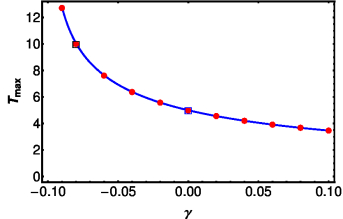
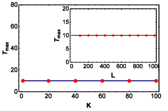
Figure 1: (Color Online) Left panel: Numerical blow-up time for the plane wave initial data (3.1) against its analytical upper bound (3.6), as a function of $\gamma\in[-0.09,0.1]$, for $\delta=0.1$, $\mu=\nu=0.01$, $\sigma_{R}=0.02$, $\beta=1$. Continuous (blue) curve depicts the analytical upper bound and (red) dots the numerical blow-up time. Here $L=100$, while $K=10$, $\epsilon=1$ for the cw. The analytical upper bound for $\gamma=0$ is marked by the (blue) square. Right panel: Independence of the blow-up time on the wave number $K$ for cw initial data and on the length $L$ of the spatial interval (inset). Here, $\gamma=-0.08$, the rest of parameters are as above, and for fixed $L=100$, $K\in[10,100]$ (main panel), while for fixed $K=10$, $L\in[100,1000]$ (inset). For this set of parameters, the analytical upper bound for the blow-up time is $T_{\mathrm{max}}=10.05$ (lines-marked by the black square in the upper figure), while the numerical blow-up time is $T_{\mathrm{num}}\approx 10.01$ (dots).

The left panel of Fig. 1, illustrates the comparison of the analytical upper bound on the collapse time (3.6), against its numerical value, as a function of the parameter $\gamma$, fixing the rest of parameters at specific examples of values. We observe that the analytical upper bound seems to be a very accurate estimate of the numerical collapse time, and is almost saturated. This, one would argue, is not surprising provided that the solution preserves its plane wave structure, since the latter indeed saturates the Cauchy-Schwarz inequality (2.9) used to derive our differential inequality from which the collapse time was obtained. Indicative of the accuracy of the analytical estimate is the comparison between the analytical upper bound for the case $\gamma=0$, and the numerical blow-up time for the considered set of parameters: the analytical value (3.8) is $T_{\mathrm{max}}[0.1,1]$=5 (marked by the blue square in the figure), and the numerical blow-up time (the red dot inside the square) is $T_{\mathrm{num}}=4.99$. The analytical upper bound (3.6) does not depend on the wavenumber $K$ and the half-length $L$ of the symmetric spatial interval $[-L,L]$. This independence is also preserved by the numerical blow-up time as illustrated in the right panel of Fig. 1. The observed independence is justified by the same reasons as above (i.e., that the inequality of (2.9) is indeed an equality for this type of solutions, provided they maintain their spatial form).

Figure 2, illustrates the comparison of the analytical upper bound on the collapse time (3.6) against the numerical collapse time, as a function of the parameter $\delta>0$, the amplitude of the plane wave $\epsilon$, and the parameters $\sigma_{R}$, $\beta$, $\mu$, and $\nu$. In the upper panel, we observe again the high accuracy of the analytical upper bound for the collapse time (3.6), as a function of the nonlinear gain/loss parameter $\delta$, and as a function of the amplitude $\epsilon$. In the bottom panel, we illustrate the independence of the numerical blow-up time from the parameters $\sigma_{R}$, $\beta$, $\mu$ and $\nu$, as predicted by the analytical estimate. We remark that the last two terms of the nonlinearity of (1.1) can been written as

$$F[u]=[(\mu+\nu)-\mathrm{i}\sigma_{R}]|u|^{2}u_{x}+[(\mu+\nu)-\mathrm{i}\sigma_{R}]u^{2}\overline{u}_{x}.$$

Thus, we have integrated the system varying the sum $\mu+\nu$.

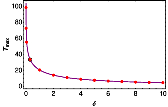
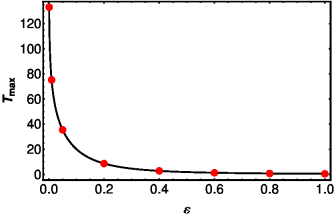
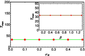
Figure 2: (Color Online) Top left panel: Numerical blow-up time for the cw initial data (3.1) against its analytical upper bound (3.6), as a function of $\delta\in[0.001,10]$, for $\gamma=0.04$, $\mu=\nu=0.01$, $\sigma_{R}=0.02$, $\beta=1$. The continuous (purple) curve corresponds to the analytical upper bound (3.6) and (red) dots to the numerical blow-up time. Here, $L=100$, while $K=10$, $\epsilon=0.1$ for the cw. Top right panel: Numerical blow-up time (dots) against the analytical upper bound (continuous (black) curve) as a function of $\epsilon\in[0.001,1]$, for $\gamma=0.04$, $\delta=1$, $\mu=\nu=0.01$, $\sigma_{R}=0.02$, $\beta=1$, $L=100$, $K=10$. Bottom left panel: Independence of the blow-up time on the parameters $\sigma_{R}$ and $\beta$ (inset). Here, $\gamma=0.04$, $\delta=0.3$, $\epsilon=0.1$, $K=10$, $L=100$; the analytical upper bound for the blow-up time (black circles) is $T_{\mathrm{max}}=33.28$. (lines), is marked by the black circle in the top panels. In the main panel, $\beta=1$, and $\sigma_{R}\in[0.01,0.5]$, while $\sigma_{R}=0.3$, $\beta\in[0.1,1.3]$ in the inset. The numerical blow-up time is $T_{\mathrm{num}}\approx 33.21$ (dots). Bottom right panel: Independence of the blow-up time on parameters $\mu+\nu\in[0.01,0.5]$, for $\beta=1$, $\sigma_{R}=0.3$; the rest of parameters are as in the upper right panel.

In Fig. 3, we present the results of a numerical study testing the behavior of the critical value (3.7) for the linear gain/loss parameter $\gamma$, as a separatrix between global existence and collapse. The left panel shows the evolution of the density for plane wave initial data (3.1), for the parameters example of the upper panel of Fig. 1, and the choice of the parameter $\gamma$ exactly at the critical value, $\gamma=\gamma^{*}=-0.1$. We observe the blow-up of the density, found numerically at time $T_{\mathrm{num}}=27.56$. The collapse is similar to that of an unstable cubic ordinary differential equation (ODE), with a rapid, spatially uniform, monotonic increase of the density as the evolution approaches the collapse time. Notice the preservation (both in this case and in the case discussed below) of the plane wave character of the solution. On the other hand, slightly perturbing the parameter $\gamma<\gamma^{*}$, we observe the complete change in the asymptotic behavior, exhibiting the decay of solutions. This is shown in the right panel, illustrating the evolution of the density for plane wave initial data for the parameters example of the upper panel, but for $\gamma-0.101<\gamma^{*}=-0.1$, slightly below from the critical value $\gamma^{*}$. The decay is again spatially uniform, resembling this time, that of a stable cubic ODE. We observe that the time-scales for blow-up (2.15) —and (3.6) in the case of the plane wave initial data— coincide with the time-scales for blow-up of the background $h^{2}$ (3.5). Furthermore, it follows from the solution (3.4) that $\lim_{t\rightarrow\infty}h(t)^{2}=0$, if $\gamma<-\delta h_{0}^{2}$, for $\delta>0$, i.e., the condition for decay of the background $h(t)$ coincides with the condition $\gamma<\gamma^{*}$ for the decay of the solution in the regime $\gamma<0,\,\delta>0$. This coincidence explains the saturation of the analytical upper bound (3.6) by the numerical blow-up times from a complementary perspective (to that of the saturation of the inequality of Eq. (2.9)) and the overall agreement of the parametric dependencies between the numerics and the theoretical analysis above.

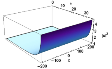
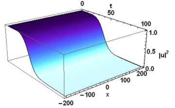
Figure 3: (Color Online) Left Panel: Collapse of the density $|u|^{2}$ for plane-wave initial data (3.1), as found for $\delta=0.1$, $\epsilon=1$, and the critical value for $\gamma=\gamma^{*}-0.1$. The rest of parameters are $K=10$, $L=200$, $\mu=0.01$, $\nu=0.01$, $\sigma=0.02$, $\beta=1$. Right Panel: Decay of the density $|u|^{2}$ for plane-wave initial data, as found for $\delta=0.1$, $\epsilon=1$, and $\gamma=-0.101<\gamma^{*}-0.1$. The rest of parameters are the same as in the upper panel.

3.2 Decaying (sech-profiled) initial conditions.

The second example for our numerical study concerns sech-profiled initial data

$$u_{0}(x)=\epsilon\,\mathrm{sech}x,$$ (3.9)

of amplitude $\epsilon>0$. Such initial data correspond to the profile of a “bright soliton” as an initial state. In this case,

$$M(0)=\frac{1}{2L}\int_{-L}^{L}\epsilon^{2}\mathrm{sech}^{2}xdx=\frac{\epsilon^{2}\mathrm{tanh}L}{L},$$

and Theorem 2.2 and (2.15) assert that the analytical upper bound of the collapse time $T_{\mathrm{max}}[\gamma,\delta,M(0)]$ is

$$T_{\mathrm{max}}[\gamma,\delta,\epsilon,L]=\frac{1}{2\gamma}\log\left[1+\frac{\gamma L}{\delta\epsilon^{2}\mathrm{tanh}L}\right].$$ (3.10)

Also, (2.19) asserts that the analytical upper bound for the collapse time in the case $\gamma=0$ is

$$T_{\mathrm{max}}[\delta,\epsilon,L]=\frac{L}{2\delta\epsilon^{2}\mathrm{tanh}L}.$$ (3.11)

According to (2.16), the critical value $\gamma^{*}$ in this case [cf. (3.10)] is:

$$\gamma^{*}=-\frac{\delta\epsilon^{2}\mathrm{tanh}L}{L}.$$ (3.12)

Moreover, it follows from (3.12), that for a sufficiently large half-length parameter $L$,

$$\gamma^{*}\approx 0.$$ (3.13)

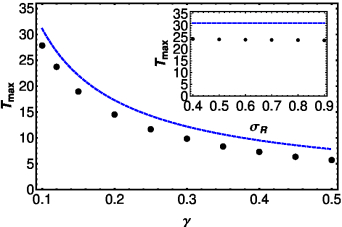
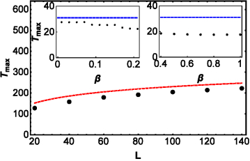
Figure 4: (Color Online) Left panel: Numerical blow-up time for the $\mathrm{sech}$-profiled initial data (3.9) against its analytical upper bound (3.10), as a function of $\gamma\in[0.1,0.5]$. Parameters $\delta=0.01$, $\mu=\nu=0.01$, $\sigma_{R}=0.02$, $\beta=0.02$. The dashed (blue) curve is traced for the analytical upper bound (3.10) and (black) dots for the numerical blow-up time; here $L=50$. The inset illustrates the numerical blow-up time (dots) against the analytical upper bound (dashed (blue) curve) as a function of $\sigma_{R}\in[0.4,1]$. Parameters $\gamma=0.1$, $\delta=0.01$, $\mu=\nu=0.01$, $\sigma_{R}=0.02$, $\beta=0.02$, $L=50$. Right panel: Numerical blow-up time for the $\mathrm{sech}$-profiled initial data (3.9) against its analytical upper bound (3.10), as a function of $L\in[20,140]$. Parameters $\gamma=0.01$, $\delta=0.01$, $\mu=\nu=0.01$, $\sigma_{R}=0.02$, $\beta=0.02$. The dashed (red) curve is traced for the analytical upper bound (3.10) and (black) dots for the numerical blow-up time. The insets illustrate the numerical blow-up time (dots) against the analytical upper bound (dashed (blue) curve) as a function of $\beta\in[0.01,0.2]$ (left inset) and $\beta\in[0.4,1]$ (right inset) . Parameters $\gamma=0.1$, $\delta=0.01$, $\mu=\nu=0.01$, $\sigma_{R}=0.02$, $\beta=0.02$, $L=50$.

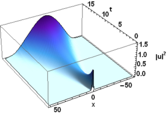
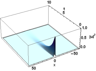
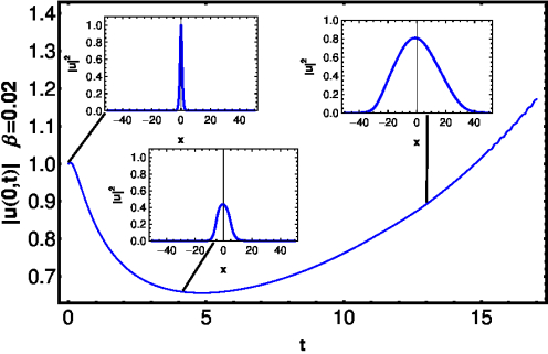
Figure 5: (Color Online) Dynamics for $\mathrm{sech}$-type initial data, for $\beta=0.02$, $\delta=0.01$, $\epsilon=1$, $\mu=0.01$, $\nu=0.01$, $\sigma=0.02$, and $L=50$. Upper left panel: Evolution of the density $|u|^{2}$ towards collapse, when $\gamma=0.1>\gamma^{*}\approx 0$. Upper right panel: Decay of the density $|u|^{2}$ when $\gamma=-0.1<\gamma^{*}\approx 0$. Bottom panel: Evolution of $|u(0,t)|$ for the center of the pulse towards collapse when $\gamma=0.1>\gamma^{*}\approx 0$, corresponding to the density evolution shown in the upper left panel. The insets demonstrate snapshots of the density $|u|^{2}$ for specific values of $|u(0,t)|$-marked by lines connecting the density profiles.

In the left panel of Fig. 4, we present the numerical study on the comparison of the numerical blow-up time for the $\mathrm{sech}$-profiled initial data (3.9), against its analytical upper bound (3.10), as a function of $\gamma\in[0.1,0.5]$. The rest of parameters are $\delta=0.01$, $\mu=\nu=0.01$, $\sigma_{R}=0.02$, $\beta=0.02$ and $L=50$. We observe that the analytical upper bound is again satisfied. However, it is not saturated as in the case of the cw initial data (as discussed above). Here, the time of collapse differs systematically by about $15$-$30$%, suggesting the potential for more interesting dynamical evolutions that we now explore. In fact, the case of the sech-profiled initial data, is much different since the initial data are spatially localized. By continuity, the solution will be also spatially localized for a finite interval $[0,\tau]$ prior to collapse. In this case, for the height of the wave-background we have $h(t)^{2}=0=\min_{x\in[-L,L]}|u(x,t)|^{2}$ —the minimum of the density of the solution. Also, in this case we have the inequality

$$e^{-2\gamma t}h(t)^{2} < M\left(t\right)=\frac{{{e}^{-2\gamma t}}}{2L}\int_{-L}^{L}|u(x,t)|^{2}dx$$ (3.14)

$$< \frac{{{e}^{-2\gamma t}}}{2L}\max_{x\in[-L,L]}|u(x,t)|^{2}\,2L$$

$$=e^{-2\gamma t}\max_{x\in[-L,L]}|u(x,t)|^{2},$$

satisfied by the amplitude $\max_{x\in[-L,L]}|u(x,t)|^{2}$ of the localized solution, for all $\;\;t\in[0,\tau]$. Thus, in the case of spatially localized data, we expect that the collapse will be predominately manifested as the increase of the amplitude, which grows faster than the averaged norm $M(t)$, due to (3.14). Consequently, the amplitude may be expected to blow-up at an earlier time than $M(t)$.

It is also interesting to remark the slow logarithmic increase of the numerical blow-up time with respect to the parameter $L\in[20,140]$, as predicted by the analytical upper bound (3.10), and shown in the right panel of Fig. 4 i.e., although the quantitative collapse time may be different, qualitatively our expression very accurately captures the relevant functional dependences. The parameter values for this example are $\gamma=0.01$, $\delta=0.01$, $\mu=\nu=0.01$, $\sigma_{R}=0.02$, $\beta=0.02$.

The insets in both panels of Fig. 4 examine numerically the independence of the collapse time on others among the rest of the nonlinear parameters. In both examples we have considered the analytical upper bound $T_{\mathrm{max}}=31$, for $\gamma=0.1$, $\delta=0.01$, $\mu=\nu=0.01$, $\sigma_{R}=0.02$, $\beta=0.02$, and $L=50$. The inset in the left panel shows the small variations of the numerical blow-up time with respect to $\sigma_{R}\in[0.4,1]$, around a mean constant value $T_{\mathrm{num,\sigma_{R}}}\approx 24$. The left inset in the right panel shows a ”decreasing step function” effect for the numerical blow-up time with respect to $\beta\in[0.01,0.2]$, while the right inset shows that the numerical blow-up time has reached a mean constant value $T_{\mathrm{num},\beta}\approx 17.8$ when $\beta\in[0.4,1]$. The difference between $T_{\mathrm{num,\sigma_{R}}}$ and $T_{\mathrm{num},\beta}$ suggests that the real blow-up time may jump to different numerical values as the nonlinear parameters $\beta,\sigma_{R}$ vary (the behavior for $\mu,\nu$ is similar), although remaining constant within specific intervals of variation. This effect may be related to transition between different dynamics of the initial pulse prior to collapse, as will be shown below.

In Fig. 5, we present the results of a numerical study verifying that (3.13) is an approximate critical point separating global existence from collapse. Parameter values used for this study are $\beta=0.02$, $\delta=0.01$, $\epsilon=1$, $\mu=\nu=0.01$, $\sigma_{R}=0.2$ and $L=50$. The left upper panel illustrates the evolution of the initial density (3.9) for $t\in[0,15]$, with $\gamma=0.1>\gamma^{*}\approx 0$, towards collapse at time $T_{\mathrm{num}}=27.85$ ($<T_{\mathrm{max}}=31$ —the analytical upper bound). We observe a nontrivial collapse mechanism, characterized (after a transient stage) by a self-similar evolution.

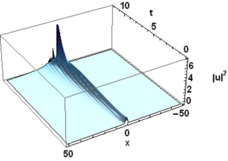
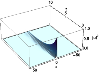
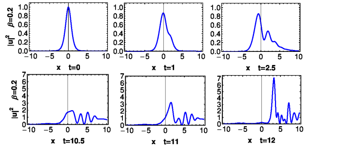
Figure 6: (Color Online) Dynamics for $\mathrm{sech}$-type initial data, when $\beta=0.2$. The rest of parameters are fixed as in Fig. 5. Upper left panel: Evolution of the density $|u|^{2}$ towards collapse, when $\gamma=0.1>\gamma^{*}\approx 0$. Upper right panel: Decay of the density $|u|^{2}$ when $\gamma=-0.1<\gamma^{*}\approx 0$. Bottom panel: Snapshots of the density $|u|^{2}$ towards collapse when $\gamma=0.1>\gamma^{*}\approx 0$, corresponding to the density evolution shown in the upper left panel.

Initially, the pulse amplitude is decreased but its width is increased (i.e., the pulse tends to disperse); nevertheless, as the gain mechanisms start playing a crucial role in the dynamics, the effect on the amplitude is reversed, and both width and amplitude grow self-similarly towards a collapsing state. To highlight this behavior, we show in the bottom panel the evolution of $|u(0,t)|$ of the center of pulse for $t\in[0,20]$. The amplitude decays and after reaching a minimum, it starts growing. The insets are showing specific snapshots of the density $|u|^{2}$ corresponding to specific times and values of norm. The first one, shows the initial condition at $t=0$, while the second shows the density profile at $t=4$, where the amplitude has decreased and the width of the pulse has increased. The last one shows the density profile at $t=13$, where both amplitude and width have increased, and the pulse evolves towards collapse. On the other hand, as shown in the upper right panel of Fig. 5, when $\gamma=-0.1<\gamma^{*}$ the initial density decays at an exponential rate. This decay still occurs in a self-similar manner, where the amplitude of the pulse decays faster than the increase of its width. Similar dynamics towards collapse (or decay) have been observed for small variations of $\beta$, as well as of the rest of the nonlinear parameters.

Larger variations of these parameters may lead to a different type of transient dynamics towards collapse or decay. In Fig. 6, we present the study for $\beta=0.2$ and the rest of parameters fixed as in Fig. 5. The top left panel shows the evolution of the initial density (3.9) for $t\in[0,12]$ towards collapse. The numerical blow-up time is decreased further to $T_{\mathrm{num}}=20.89$, and the dynamics is very different from the self-similar evolution of the previous case, due to the considerable dispersion effect. This difference is highlighted in the bottom panel, showing snapshots of the density profiles at specific times, prior to collapse. The initial pulse is decomposed to a “core pulse” of decreased amplitude and a nonlinear wave train, both traveling to the right at slow speed (upper row). Progressively (bottom rows), and as the gain becomes more prominent, the amplitudes of the core and of the decomposed waves start increasing (note the change of scaling in the amplitude axis). While at a particular time instant, the amplitude of the wave-train is almost reaching that of the core, as shown in the snapshot for $t=10.5$, eventually the core gains amplitude in comparison with the rest of the waves, as shown in the snapshot for $t=11$. A sudden increase of the amplitude of the core is observed at $t=12$, leading to collapse. For further variations of the parameter $\beta$, the numerical blow-up time is stabilized —an effect illustrated in the inset of the right panel of Fig. 4— and the collapse dynamics were found to be similar. The top right panel present the results of the numerical study for $\gamma=-0.1<\gamma^{*}$. The initial pulse is again decomposed to a wave train, but now the dynamics are reversed to decay instead of collapse.

3.3 Non decaying (tanh²-profiled) initial conditions.

The third example of initial condition which we shall examine is the case of tanh²-profiled initial data,

$$u_{0}(x)=\epsilon\,\mathrm{tanh}^{2}x,$$ (3.15)

of amplitude $\epsilon>0$ (here, the discussion on the values of the derivatives on the boundaries should be recalled). Such initial data resemble a density ($|u|^{2}$) profile reminiscent of the intensity dip of a dark soliton of the defocusing NLS, on the top of the cw background, which is compliant with our periodic boundary conditions. Note, that a simpler ${\rm tanh}$-type initial condition (real or complex to model the black or gray solitons of the NLS) would violate our periodic boundary conditions (and would require a different type of boundary conditions, such as Neumann). While the observations here are still valid for the latter case, we will report corresponding results in a future communication. For the initial data (3.15),

$$M(0)=\frac{1}{2L}\int_{-L}^{L}\epsilon^{2}\mathrm{tanh}^{4}xdx=\epsilon^{2}\left[\frac{3L-(3+\mathrm{tanh}^{2}L)\mathrm{tanh}L}{3L}\right].$$

Thus, in the present case, Theorem 2.2 and (2.15) assert that the analytical upper bound of the collapse time $T_{\mathrm{max}}[\gamma,\delta,M(0)]$ is

$$T_{\mathrm{max}}[\gamma,\delta,\epsilon,L]=\frac{1}{2\gamma}\log\left[1+\frac{3\gamma L}{\delta\epsilon^{2}[(3L-(3+\mathrm{tanh}^{2}L)\mathrm{tanh}L]}\right].$$ (3.16)

Then, (2.19) asserts that the analytical upper bound for the collapse time in the case $\gamma=0$ is

$$T_{\mathrm{max}}[\delta,\epsilon,L]=\frac{3L}{2\delta\epsilon^{2}[(3L-(3+\mathrm{tanh}^{2}L)\mathrm{tanh}L]}.$$ (3.17)

Furthermore, Eq. (2.16), implies that the critical value $\gamma^{*}$ in the present case [see (3.16)] is:

$$\gamma^{*}=-\delta\epsilon^{2}\left[\frac{3L-(3+\mathrm{tanh}^{2}L)\mathrm{tanh}L}{3L}\right].$$ (3.18)

It is interesting to recover that for a sufficiently large $L$, the initial value of the functional $M(t)$ at $t=0$ (3.15), the analytical upper bounds for the collapse time (3.16) and (3.17), and the critical value $\gamma^{*}$ given in (3.18), approximate the relevant values for the example of the plane-wave initial conditions discussed in Sec. 3.1. Namely, for large $L$,

$$M(0)\approx\epsilon^{2},\;\;T_{\mathrm{max}}[\gamma,\delta,\epsilon,L]\approx\frac{1}{2\gamma}\log\left[1+\frac{\gamma}{\delta\epsilon^{2}}\right],\;\;\mbox{for $\gamma\neq 0$},$$ (3.19)

$$T_{\mathrm{max}}[\gamma,\delta,\epsilon,L]\approx\frac{1}{2\delta\epsilon^{2}},\;\;\mbox{for $\gamma\neq 0$},\;\;\mbox{and}\;\;\gamma^{*}\approx-\delta\epsilon^{2}.$$ (3.20)

This result is of course not surprising given that the fact that as $L$ increases the weight nature of the average in the definition of $M(0)$ yields a progressively vanishing contribution from the localized part of the relevant initial condition profile. The approximations (3.19) and (3.20) may indicate that the numerical collapse times may not only respect, but also be much closer to their analytical upper bounds as in the case of the plane-wave initial data. Another feature, interesting by itself, which may support the above argument, is that the collapse may be manifested by the collapse of the wave background for small values of the dispersion parameter $\beta$ and of the nonlinear parameters, as discussed in Sec. 3.1. This fact should be also supported by the expectation that the dip of the density profile should have a little effect to the averaged norm $M(t)$, and the main contribution should come from the wave background. More precisely, the approximate equation on the evolution of $M(t)$ should be also valid in the case of the initial data (3.15).

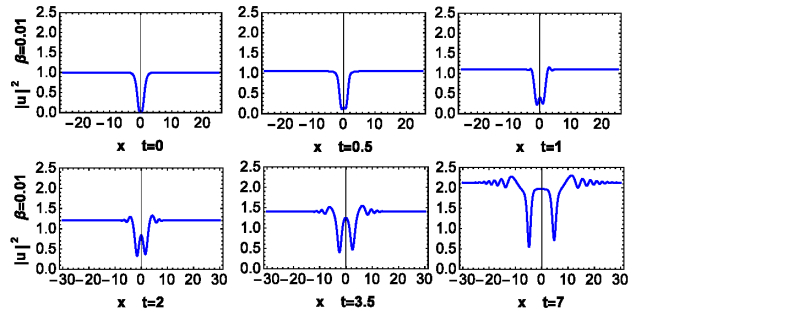
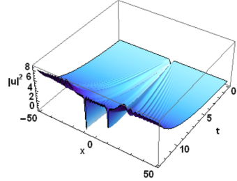
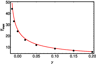
Figure 7: (Color Online) Upper panel: Snapshots of the evolution of the density $|u|^{2}$ towards collapse for $\mathrm{tanh^{2}}$-type initial data, when $\delta=0.02$, $\epsilon=1$ and $\gamma=0.025>\gamma^{*}=-0.02$. The rest of parameters are $L=50$, $\mu=0.01$, $\nu=0.01$, $\sigma=0.02$, $\beta=0.01$. Bottom left panel: An upper view for the collapse of the density $|u|^{2}$ for $\mathrm{tanh^{2}}$-type initial data for the set of parameters of the upper panel. Bottom right panel: Comparison of the analytical upper bound (3.16) (dashed (red) curve) against the numerical blow-up time (dots) as a function of $\gamma$. Rest of parameters are fixed as in the study of the upper panel.

In the top and bottom left panel of Fig. 7, we present the numerical results on the evolution of the density of initial data (3.15), for $\epsilon=1$, $\gamma=0.025$ and $\delta=0.02$. The rest of parameters are $\mu=0.01$, $\nu=0.01$, $\sigma=0.02$, $\beta=0.01$, and the system is integrated for $L=50$. For the given values of parameters, the critical value $\gamma\approx-0.02<0$, and since $\gamma>\gamma^{*}$, we are in the regime of finite-time collapse. The top panel shows snapshots of the density profiles at specific times, and the bottom left panel shows a (bottom) view of the density evolution, prior to collapse. The increase of the density is manifested by the increase of the height of the wave-background and accompanied by the nontrivial dynamics of the initial dip, prior to collapse at numerical time $T_{\mathrm{num}}=15.9$, while the analytical upper bound is $T_{\mathrm{max}}=16.5$. As highlighted in the upper panel, the initial density dip appears to separate into two traveling (at low speed) dark pulses of progressively increasing depths, emitting radiation in the form of linear waves of increasing amplitude. In fact, the emerging patterns bearing an oscillatory wavefront, together with a solitary wave are reminiscent of dispersive shock waves (DSWs) [33]. The generation of two dark soliton pulses can be understood by the fact that the initial condition has a trivial phase profile (i.e., does not have the phase jump needed for a dark soliton); thus, the initial dip separates into two dark solitons moving to opposite directions so that the phase of one soliton is compensated by the other soliton, with the total phase retaining its initial asymptotic structure – see, e.g., Ref. [34]. On the other hand, the clearly observed asymmetry in the evolution profile is apparently produced by parity breaking terms, such as the first and third spatial derivatives in Eq. (1.1). The bottom right panel of Fig. 7 shows the comparison of the analytical upper bound (3.16) (dashed (red) curve) against the numerical blow-up time (dots) as a function of $\gamma$, when the rest of parameters are fixed as in the study of the upper panel. We observe that the numerical blow-up are quite close to their analytical upper bounds, similarly (for the reasons indicated above) to the plane wave case.

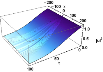
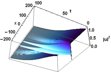
Figure 8: (Color Online) Left panel: An upper view for the decay of the density $|u|^{2}$ for $\mathrm{tanh^{2}}$-type initial data, as found for $\delta=0.02$, $\epsilon=1$, and $\gamma=-0.025<\gamma^{*}=-0.02$. The rest of parameters are $L=200$, $\mu=0.01$, $\nu=0.01$, $\sigma=0.02$, $\beta=1$. Right panel: A bottom view for the decay of the density $|u|^{2}$ for $\mathrm{tanh^{2}}$-type initial data. Parameters as in the upper panel.

In Fig. 8, keeping the rest of parameters as above and integrating the system for $L=200$, we present the results of the numerical study for slightly perturbing the parameter $\gamma$ from its critical value $\gamma^{*}=-0.02$, falling within the decay regime, e.g, by considering $\gamma=-0.025$. The left (right) panel shows a top (bottom) view of the evolution of the density manifested by the decay of the height of the wave-background again accompanied by nontrivial dynamics of the initial dip, prior to decay: it separates again into two traveling (at low speed) dark pulses, this time of slowly decreasing depths. The two decaying pulses are emitting radiation again, which also decays, following the decay of the wave-background. Once again, on both sides the oscillatory waveforms coupled to the dark solitary waves are somewhat reminiscent of DSW patterns.

For larger valued-parametric regimes of the higher-order effects, the transient dynamics prior to collapse or decay were found to be potentially quite different. Concerning collapse, we have recovered the same effect for the variation of the numerical blow-up time associated with the transition to a different type of collapsing dynamics. In Fig. 9, we present snapshots of the density evolution for $\sigma_{R}=0.2$ and the rest of the parameters fixed as in the case of Fig. 7 —the case of collapse. While the initial dark pulse is still separated into two dips as explained above, we also observe stronger “one-sided” radiation to the left, due to the third-order dispersion, which is increased due to the (relatively strong) Raman effect. The two dips and the right-part of the background seem to have a similar dynamics as in the case of Fig. 7, however the collapse is manifested by the sudden increase of the amplitudes of the oscillatory waveforms in the background formed to the left of the dips.

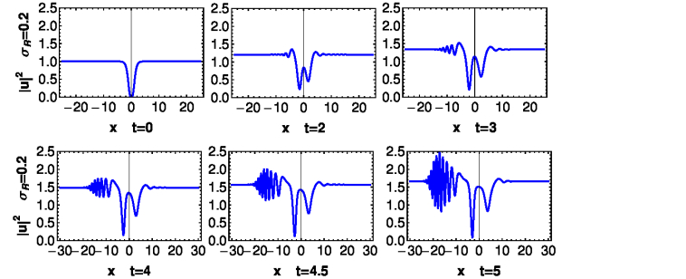
Figure 9: (Color Online) Snapshots of the evolution of the density $|u|^{2}$ towards collapse when $\gamma=0.025>\gamma^{*}=-0.02$, all the parameters fixed as in the study of Fig. 7, but for the increased value of $\sigma_{R}=0.2$.

The transient dynamics of our system can be very rich. As an example, in Fig. 10 we show a contour plot of the space-time evolution of the density $|u|^{2}$ in the decay regime $\gamma=-0.025<\gamma^{*}=-0.02$ (the rest of parameters fixed as in the study of Fig. 8), but for increased dispersion effect, namely $\beta=0.2$. The initial dip is decomposed to an almost spatially periodic pattern, traveling to the left. These periodic structures, in turn, have different survival times prior to the their final decay. A more detailed study of such phenomenology is warranted although it is outside the scope of the present investigation.

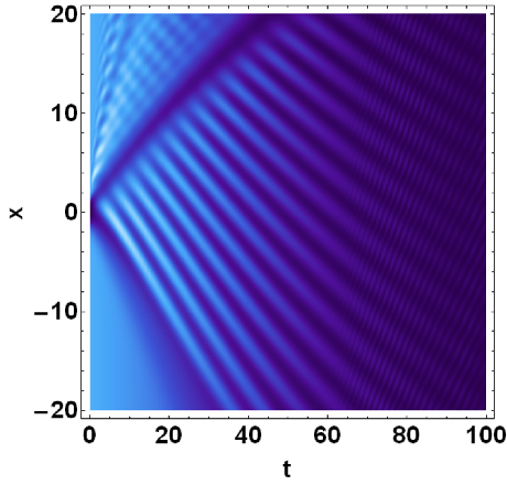
Figure 10: (Color Online) Contour plot of the evolution of the density $|u|^{2}$ for $\gamma=-0.025<\gamma^{*}$ and $\beta=0.2$. The rest of the parameters is fixed as in the the example of Fig. 8.

4 Conclusions

In this work, analytical studies corroborated by numerical simulations, considered the collapse dynamics of the higher-order NLS equation (1.1) supplemented by periodic boundary conditions. The model has important applications in describing the evolution of ultrashort pulses in nonlinear media (such as optical fibers, metamaterials, water waves), where linear and nonlinear gain/losses and higher order conservative and dissipative effects are of importance. We have shown by means of simple analytical energy arguments and verified numerically, that the collapse/decay dynamics are chiefly dominated by the linear and nonlinear gain/loss of strength $\gamma$ and $\delta$ respectively. We identified a critical value $\gamma^{*}$ in the regime $\gamma<0$, $\delta>0$, which is separating finite-time collapse from the decay of solutions. An important conclusion regarding this regime, is related to the fate of localized solutions such as pulse and dip-type waveforms [19]: referring to their true long-time dynamics, such states only survive for relatively short times, as they are subject to either catastrophic collapse or to eventual decay for generic parameter values.

The results of the numerical simulations for a variety of initial conditions suggest a very good agreement between the analytical estimates for the collapse times and the numerical ones, as well on the accuracy of the critical value $\gamma^{*}$. This agreement was excellent for plane wave initial data, and very good for waveforms bearing a density dip, while it was less good in the case of initial data resembling bright solitary wave structures, for reasons explained in the text. Furthermore, the numerical simulations gave insight on the role of the strengths of the higher order effects on the transient dynamics prior to collapse or decay, which were found to be essentially different. They have also indicated that these strengths may seriously affect the survival times of the solutions.

Our results pave the way for a better understanding of the dynamics of the considered higher-order NLS equation. An interesting direction is to discuss the collapse dynamics for the case of $s=-1$. It is also certainly relevant, to explore the associated dynamics in the stabilization regime $\gamma>0$, $\delta<0$ respectively (see [21] for some recent results), depending on the higher-order effects and the type of initial data. Future investigations should also consider the possibility of collapse of higher-order norms, and the effect on this type of collapse of the higher-order nonlinear terms, as well as of higher-dimensional settings, which may further modify the dynamical regimes analyzed herein.

Appendix A Derivation of Eq. (2.8)

Here, for the sake of completeness, we provide details for the derivation of Eq. (2.8) and also explain the choice of the functional $M(t)$ [cf. Eq. (2.3)].

First we note that the second term on the right-hand side of Eq. (2.7), after substituting $u_{t}$ by the right-hand side of Eq. (1.1) becomes:

$$\frac{e^{-2\gamma t}}{L}\mathrm{Re}\int_{-L}^{L}u_{t}\overline{u}dx=\frac{e^{-2\gamma t}}{L}\sum_{k=1}^{7}J_{k},$$ (1.1)

where

$$J_{1}=-\mathrm{Re}\left\{\frac{\mathrm{i}}{2}\int_{-L}^{L}u_{xx}\overline{u}dx\right\},\,J_{2}=\mathrm{Re}\left\{\mathrm{i}\int_{-L}^{L}|u|^{2}u\overline{u}dx\right\},$$

$$J_{3}=\mathrm{Re}\left\{\gamma\int_{-L}^{L}u\overline{u}dx\right\},\qquad J_{4}=\mathrm{Re}\left\{\delta\int_{-L}^{L}|u|^{2}u\overline{u}dx\right\},$$

$$J_{5}=\mathrm{Re}\left\{\beta\int_{-L}^{L}u_{xxx}\overline{u}dx\right\},\;\;J_{6}=\mathrm{Re}\left\{\mu\int_{-L}^{L}(|u|^{2}u)_{x}\overline{u}dx\right\},$$

$$J_{7}=\mathrm{Re}\left\{\int_{-L}^{L}(\nu-\mathrm{i}\sigma_{R})(|u|^{2})_{x}u\overline{u}dx\right\}.$$

Integration by parts and use of periodicity, implies that $J_{5}=-J_{5}$, hence $J_{5}=0$. By the same token, we have that $\int_{-L}^{L}(|u|^{2})_{x}|u|^{2}dx=0$, hence,

$$J_{6} = \mu\mathrm{Re}\int_{-L}^{L}(|u|^{2})_{x}u\overline{u}dx+\mu\mathrm{Re}\int_{-L}^{L}|u|^{2}u_{x}\overline{u}dx$$

$$= \mu\mathrm{Re}\int_{-L}^{L}(|u|^{2})_{x}|u|^{2}dx+\mu\int_{-L}^{L}|u|^{2}\mathrm{Re}(u_{x}\overline{u})dx$$

$$= \mu\mathrm{Re}\int_{-L}^{L}(|u|^{2})_{x}|u|^{2}dx+\frac{\mu}{2}\mathrm{Re}\int_{-L}^{L}(|u|^{2})_{x}|u|^{2}dx=0,$$

$$J_{7} = \mathrm{Re}\left\{(\nu-\mathrm{i}\sigma_{R})\int_{-L}^{L}(|u|^{2})_{x}|u|^{2}dx\right\}=0.$$

Similarly, we have that $J_{1}=\mathrm{Re}\left\{\frac{\mathrm{i}}{2}\int_{-L}^{L}|u_{x}|^{2}dx\right\}=0$, and $J_{2}=\mathrm{Re}\left\{\mathrm{i}\int_{-L}^{L}|u|^{4}dx\right\}=0$, as well. Thus, we recover that the only contribution to (1.1) comes from the terms $J_{3}=\gamma\int_{-L}^{L}|u|^{2}dx$, and $J_{4}=\delta\int_{-L}^{L}|u|^{4}dx$. Inserting all the above relations to (1.1), we observe that the latter is actually

$$\frac{e^{-2\gamma t}}{L}\mathrm{Re}\int_{-L}^{L}u_{t}\overline{u}dx=\gamma\frac{e^{-2\gamma t}}{L}\int_{-L}^{L}|u|^{2}dx+\delta\frac{e^{-2\gamma t}}{L}\int_{-L}^{L}|u|^{4}dx,$$ (1.2)

and consequently, Eq. (2.7) results in Eq. (2.8).

Finally, we remark that following computations similar to the above, but for the (squared) $L^{2}$-norm functional, we find that:

$$\frac{d}{dt}\int_{-L}^{L}|u|^{2}dx=2\gamma\int_{-L}^{L}|u|^{2}dx+2\delta\int_{-L}^{L}|u|^{4}dx.$$ (1.3)

Thus, it is evident that the factor $\exp(-2\gamma t)$ is the integrating factor for the linear part of the above equation. For $\gamma=\delta=0$, Eq. (1.3) is nothing but the conservation of the $L^{2}$ norm in the standard NLS model.

References

References

- Hasegawa & Kodama [1996] A. Hasegawa and Y. Kodama, Solitons in optical communications, Oxford Univeristy Press, 1996.
- Agrawal [2003] G. P. Agrawal, Nonlinear Fiber Optics, Academic Press, 2012.
- Kivshar & Agrawal [2003] Yu. S. Kivshar and G. P. Agrawal, Optical Solitons: From Fibers to Photonic Crystals, Academic Press, 2003.
- Leblond & Mihlache [2013] H. Leblond and D. Mihalache, Phys. Rep. 523 (2013), 61.
- Frantzeskakis et al. [2014] D. J. Frantzeskakis, H. Leblond and D. Mihalache, Rom. Journ. Phys. 59 (2014), 767.
- Scalora et al. [2005] M. Scalora, M. S. Syrchin, N. Akozbek, E. Y. Poliakov, G. D’Aguanno, N. Mattiucci, M. J. Bloemer, and A. M. Zheltikov, Phys. Rev. Lett. 95 (2005), 013902.
- Wen et al. [2007] S. Wen, Y. Xiang, X. Dai, Z. Tang, W. Su, and D. Fan, Phys. Rev. A 75 (2007), 033815.
- Tsitsas et al. [2009] N. L. Tsitsas, N. Rompotis, I. Kourakis, P. G. Kevrekidis, and D. J. Frantzeskakis, Phys. Rev. E 79 (2009), 037601.
- Johnson [1977] R. S. Johnson, Proc. R. Soc. Lond. A 357 (1977), 131.
- Sedletsky [2003] Yu. V. Sedletsky, J. Exp. Theor. Phys. 97 (2003), 180.
- Slunyaev [2005] A. V. Slunyaev, J. Exp. Theor. Phys. 101 (2005), 926.
- Ikeda et al [1995] H. Ikeda, M. Matsumoto, and A. Hasegawa, Opt. Lett. 20 (1995), 1113.
- Suzuki [1971] T. Tsuzuki, J. Low Temp. Phys. 4 (1971), 441.
- Hasegawa & Tappert [1973] A. Hasegawa and F. Tappert, Appl. Phys. Lett. 23 (1973), 171.
- Kivshar & Luther Davies [1998] Yu. S. Kivshar and B. Luther-Davies, Phys. Rep. 298 (1998), 81.
- Kevrekidis et al. [2008] P. G. Kevrekidis, D. J. Frantzeskakis, and R. Carretero- González, Emergent Nonlinear Phenomena in Bose-Einstein Condensates. Theory and Experiment, Springer-Verlag, 2008.
- Carretero- González et al. [2008] R. Carretero- González, D. J. Frantzeskakis, P. G. Kevrekidis, Nonlinearity 21 (2008) R139.
- Frantzeskakis [2010] D. J. Frantzeskakis. J. Phys. A 43 (2010), 213001.
- Horikis & Frantzeskakis [2013] T. P. Horikis and D. J. Frantzeskakis, Opt. Lett. 38 (2013), 5098.
- Ablowitz et al. [2011] M. J. Ablowitz, S. D. Nixon, T. P. Horikis, and D. J. Frantzeskakis, Proc. R. Soc. A (2011) 467, 2597.
- Achilleos et al. [2015] V. Achilleos, A. R. Bishop, S. Diamantidis, D. J. Frantzeskakis, T. P. Horikis, N. I. Karachalios, and P. G. Kevrekidis, arXiv:1509.03828 (2015).
- Kato [1975] T. Kato, Quasilinear equations of evolution with applications to partial differential equations, Lecture Notes in Mathematics 448, pp. 25–70, Springer-Verlag, New York, 1975.
- Kato [1985] T. Kato, Abstract differential equations and nonlinear mixed problems, Lezione Fermiane Pisa, 1985.
- Kato & Lai [1984] T. Kato and C. Y. Lai, J. Funct. Anal. 56 (1984), 15.
- Kato [1989] T. Kato, Nonlinear Schrödinger equations. Schrödinger operators, Sønderborg, 1988, 218–263, Lecture Notes in Phys. 345, Springer, Berlin, 1989.
- Cazenave [2003] T. Cazenave, Semilinear Schrödinger equations, Courant Lecture Notes 10, Amer. Math. Soc., 2003.
- Ball [1977] J. M. Ball, Quart. J. Math. Oxford 28 (1977), 473.
- Sulem & Sulem [1999] C. Sulem and P. L. Sulem, The nonlinear Schrödinger equation. Self-Focusing and wave collapse, Springer-Verlag, 1999.
- Ozawa & Yamazaki [2003] T. Ozawa and Y. Yamazaki, Nonlinearity 16 (2003), 2029.
- Taylor [1996] M. Taylor, Partial Differential Equations III, Applied Mathematical Sciences 117, Springer-Verlag, New York, 1996.
- Karachalios et al. [2007] N. I. Karachalios, H. Nistazakis and A. Yannacopoulos, Discrete Cont. Dyn. Syst. A 19 (2007), 711.
- Achilleos et al. [2013] V. Achilleos, A. Álvarez, J. Cuevas, D. J. Frantzeskakis, N. I. Karachalios, P. G. Kevrekidis, and B. Sánchez-Rey, Physica D 244 (2013), 1.
- Hoefer and Ablowitz [2009] M. Hoefer and M. Ablowitz, Scholarpedia 4 (2009) 5562.
- Blow and Doran [1985] K. J. Blow and N. J. Doran, Phys. Lett. A, 107 (1985) 55.