Limits to the precision of gradient sensing with spatial communication and temporal integration

Abstract

Gradient sensing requires at least two measurements at different points in space. These measurements must then be communicated to a common location to be compared, which is unavoidably noisy. While much is known about the limits of measurement precision by cells, the limits placed by the communication are not understood. Motivated by recent experiments, we derive the fundamental limits to the precision of gradient sensing in a multicellular system, accounting for communication and temporal integration. The gradient is estimated by comparing a “local” and a “global” molecular reporter of the external concentration, where the global reporter is exchanged between neighboring cells. Using the fluctuation-dissipation framework, we find, in contrast to the case when communication is ignored, that precision saturates with the number of cells independently of the measurement time duration, since communication establishes a maximum lengthscale over which sensory information can be reliably conveyed. Surprisingly, we also find that precision is improved if the local reporter is exchanged between cells as well, albeit more slowly than the global reporter. The reason is that while exchange of the local reporter weakens the comparison, it decreases the measurement noise. We term such a model “regional excitation–global inhibition” (REGI). Our results demonstrate that fundamental sensing limits are necessarily sharpened when the need to communicate information is taken into account.

Cells sense spatial gradients in environmental chemicals with remarkable precision. A single amoeba, for example, can respond to a difference of roughly ten attractant molecules between the front and back of the cell Song2006 . Cells are even more sensitive when they are in a group: cultures of many neurons respond to chemical gradients equivalent to a difference of only one molecule across an individual neuron’s axonal growth cone Rosoff2004 ; clusters of malignant lymphocytes have a wider chemotactic sensitivity than single cells MaletEngra:2015jc ; and groups of communicating epithelial cells detect gradients that are too weak for a single cell to detect us_unpublished . More generally, collective chemosensing properties are often very distinct from those in individual cells Friedl:2009kz ; Dona:2013cd ; Pocha:2014ep ; MaletEngra:2015jc . These observations have generated a renewed interest in the question of what sets the fundamental limit to the precision of gradient sensing in large, spatially extended, often collective sensory systems.

Fundamentally, sensing a stationary gradient requires at least two measurements to be made at different points in space. The precision of these two or more individual measurements bounds the gradient sensing precision Berg1977 ; Goodhill1999 . In their turn, each individual measurement is limited by the finite number of molecules within the detector volume and the ability of the detector to integrate over time, a point first made by Berg and Purcell (BP) Berg1977 . More detailed calculations of gradient sensing by specific geometries of receptors have since confirmed that the precision of gradient sensing remains limited by an expression of the BP type Endres2009 ; Hu2010 ; Endres2008 .

However, absent in this description is the fundamental recognition that in order for the gradient to be measured, information about multiple spatially separated measurements must be communicated to a common location. This point is particularly evident in the case of multicellular sensing: if two cells at either edge of a population measure concentrations that are different, neither cell “knows” this fact until the information is shared. This is also important for a single cell: information from receptors on either side of a cell must be transported, e.g., via diffusive messenger molecules, to the location of the molecular machinery that initiates the phenotypic response. How is the precision of gradient sensing affected by this fundamental communication requirement?

As discussed recently in the context of instantaneous measurements us_unpublished , the communication imposes important limitations. First, detection of an internal diffusive messenger by cellular machinery introduces its own BP-type limit on gradient sensing. Since the volume of an internal detector must be smaller than that of the whole system, and diffusion in the cytoplasm is often slow, such an intrinsic BP limitation could be dramatic. Second, in addition to the detection noise, the strength of the communication itself may be hampered over long distances by messenger turnover. This imposes a finite lengthscale over which communication is reliable, with respect to the molecular noise. However, the communicating cells can integrate the signals over time Berg1977 , improving detection of even very weak messages. Whether such integration can lift the communication constraints has not yet been addressed.

To analyze constraints on gradient sensing in spatially extended systems with temporal integration, we use a minimal model of collective sensing based on the local excitation–global inhibition (LEGI) approach Levchenko2002 . This sensory mechanism uses a local and a global internal reporter of the external concentration, where only the global reporter is exchanged and averaged among neighboring cells. Comparison of the two reporters then measures if the local concentration is above or below the average, and hence whether the cell is on the high-concentration edge of the population. We analyze the model using a fluctuation-dissipation framework Bialek2005 , to derive the precision with which a chemical gradient can be estimated over long observation times. In the case where the need to communicate is ignored, the precision would grow indefinitely with the number of cells. In contrast, we find that, communication imposes limits on sensing even for long measurement times. Furthermore, the analysis reveals a counterintuitive strategy for optimizing the precision. We find that if the local reporter is also exchanged, at a fraction of the rate of the global reporter, the precision can be significantly enhanced. Even though such exchange makes the two compared concentrations more similar, which weakens the comparison, it reduces the measurement noise of the local reporter. This tradeoff leads to an optimal ratio of exchange rates that maximizes sensory precision. We discuss how the predictions of our analysis could be tested experimentally.

I Results

We discretize the spatially-extended gradient sensor into compartments. These can be whole cells or their parts, but we will refer to them as cells from now on. There is a diffusible chemical whose concentration varies linearly in space. The chemical gradient defines a direction within the sensor, and we focus on a chain of cells along this direction (Fig. 1A). Numbering the cells from $n=1$ to $N$, each cell experiences a local concentration $c_{n}=c_{N}-(N-n)ag$, where $c_{N}$ is the background concentration, $g$ is the concentration gradient, and $a$ is the linear size of each cell. We choose without loss of generality to have $g\geq 0$ and to reference the background concentration at cell $N$, which is then at the higher edge of the gradient. We focus on this cell because we imagine it will be the first to initiate a phenotypic response, such as proliferating or directed motility. Finally, we focus on the limit $ag/c_{N}\ll 1$ because limits on the sensory precision will be the most important for such small, hard to measure gradients.

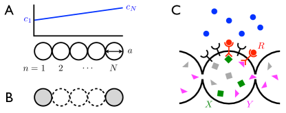
Figure 1: Spatially extended gradient sensing. (A) A chain of $N$ compartments or cells is exposed to a linear profile of a diffusible chemical. (B) In an idealized detector, the two edge cells communicate their measurements perfectly and instantly. (C) In our model, bound receptors (R) activate a local (X) and global reporter molecules (Y), and Y is exchanged between cells for the communication.

I.1 An idealized detector

First, we consider the case when the two edge cells form an idealized detector, in the sense that each cell counts every external molecule in its vicinity, and one cell “knows” instantly and perfectly the count of the other (Fig. 1B). The gradient could then be estimated by the difference in the concentration measurements made by the two cells Berg1977 ; Goodhill1999 . The mean of this difference is $\bar{\Delta}=\bar{c}_{N}-\bar{c}_{1}=(N-1)ag$, and its error is given by the corresponding errors in the two measurements, $(\delta\Delta)^{2}=(\delta c_{1})^{2}+(\delta c_{N})^{2}$, under the assumption that the measurements are independent.

Berg and Purcell showed Berg1977 that the fractional error in each measurement is not smaller than $(\delta c/\bar{c})^{2}\sim 1/(aDT\bar{c})$, where $D$ is the diffusion constant of the ligand, and $T$ is the time over which the measurement is integrated. This expression has an intuitive interpretation: the fractional error is at least as large as the Poisson counting noise, which scales inversely with the number of molecular counts. The number of counts that can be made in a time $T$ is given by the number of molecules in the vicinity of a cell at a given time, roughly $\bar{c}a^{3}$, multiplied by the number of times the diffusion renews these molecules, $T/\tau$, where $\tau\sim a^{2}/D$. This product is $aDT\bar{c}$.

The error in the gradient estimate is then given by $(\delta\Delta)^{2}\sim\bar{c}_{1}/(aDT)+\bar{c}_{N}/(aDT)$. For sufficiently small gradients, such that $\bar{c}_{1}\approx\bar{c}_{N}$, this becomes

$$\left(\frac{\delta\Delta}{\bar{c}_{N}}\right)^{2}\sim\frac{1}{aDT\bar{c}_{N}}.$$ (1)

Thus, for an idealized detector, the error in the gradient estimate is limited entirely by the error in the measurements made by each of the edge cells. In general, we could think of the measurement at either edge being performed by a region that is larger than a single cell. Since each region could not be larger than the whole system, the highest precision is obtained when $\sim$$Na$ replaces $a$ in Eqn. 1. This result has been derived more rigorously Endres2009 , and apart from a constant prefactor, Eqn. 1 indeed provides the estimation error in the limit of large detector separation and fast detection kinetics. More complex geometries, such as rings of detectors Endres2009 , or detectors distributed over the surface of a circle Hu2010 or a sphere Endres2008 , have also been considered, and Eqn. 1 again emerges as the corresponding bound, with the lengthscale $a$ replaced by that dictated by the specific geometry.

Eqn. 1 can be combined with the mean $\bar{\Delta}$ to produce the signal-to-noise ratio (SNR) for gradient detection

$$\frac{1}{{\rm SNR}}\equiv\left(\frac{\delta\Delta}{\bar{\Delta}}\right)^{2}\sim\frac{\bar{c}_{N}}{[(N-1)ag]^{2}aDT}$$ (2)

This expression again has a clear interpretation: the SNR increases if the external molecules diffuse more quickly ($D$) or are more sharply graded ($g$), or if the detectors are larger ($a$), are better separated ($N$), or integrate longer ($T$). Yet, the SNR is worse for a larger background concentration ($\bar{c}_{N}$), since it is more difficult to detect a small gradient on top of a larger background. The measures defined in Eqns. 1 and 2 are conceptually equivalent only in the case of low background concentration, when the difference $\Delta$ is comparable to the background concentration $c_{N}$ (i. e. $c_{1}\approx 0$). While much of the field has focused on Eqn. 1, here we are concerned with the opposite case: the fundamental limits to the detection of small gradients on a large background. Therefore from here on we focus on the SNR, Eqn. 2.

I.2 Accounting for the need to communicate

Eqn. 2 cannot be a fundamental limit because it neglects a critical aspect of gradient sensing: the need to communicate information from multiple detectors to a common location. Indeed, the idealized detector implies the existence of a “spooky action at a distance” Mermin1985 , i. e. an unknown, instantaneous, and error-free communication mechanism. What are the limits to gradient sensing when communication is properly accounted for?

To answer this, a model of gradient sensing must be assumed. A naive model would allow each cell access to information about the input measured and broadcast by every other cell. This would require a number of private communication channels that grows with the number of cells, which is not plausible. A realistic alternative that would involve just one message being communicated is for each cell to have access to some aggregate, average information, to which all comparisons are made. There are a few such models Meinhardt:1999uw ; Rappel:2002fb ; Jilkine:2011fy , and our choice among them is guided by the fact that collective detection of weak gradients is observed in steady state, and over a wide range of background concentration in both neurons Rosoff2004 and epithelial cells us_unpublished . This supports an adaptive spatial (rather than temporal) sensing, such as can be implemented by the local excitation–global inhibition (LEGI) mechanism Levchenko2002 .

The LEGI model is illustrated in Fig. 1C. Each cell contains receptors that bind and unbind external molecules with rates $\alpha$ and $\mu$, respectively. Bound receptors (R) activate both a local (X) and a global (Y) intracellular species with rate $\beta$. Deactivation of X and $Y$ occurs spontaneously with rate $\nu$. Whereas X is confined to each cell, Y is exchanged between neighboring cells with rate $\gamma$, which provides the cell-cell communication. X then excites a downstream species while Y inhibits it (LEGI). Conceptually, X measures the local concentration of external molecules, while Y represents their spatially-averaged concentration. If the local concentration is higher than the average (i.e., the excitation exceeds the inhibition), then the cell is at the higher edge of the gradient. While such comparison of the excitation and the inhibition can be done by many different molecular mechanisms Levchenko2002 , here we are interested in the limit of shallow gradients. In this limit, biochemical reactions doing the comparison can be linearized around the small difference of X and Y, and the comparison is equivalent to subtracting Y from X us_unpublished . Therefore, we take this difference, $\Delta$, as the readout of the model.

Because we are interested in the limits to sensory precision, we focus on the most sensitive regime, the linear response regime, where the effects of saturation are neglected. Introducing $r_{n}$, $x_{n}$, and $y_{n}$ as the molecule numbers of R, X, and Y in the $n$th cell, the stochastic model dynamics are

$$\dot{c} =D\nabla^{2}c-\sum_{n=1}^{N}\delta(\vec{x}-\vec{x}_{n})\dot{r}_{n},$$

$$\dot{r}_{n} =\alpha c_{n}-\mu r_{n}+\eta_{n},$$

$$\dot{x}_{n} =\beta r_{n}-\nu x_{n}+\xi_{n},$$

$$\dot{y}_{n} =\beta r_{n}-\nu\sum_{n^{\prime}=1}^{N}M_{nn^{\prime}}y_{n^{\prime}}+\chi_{n},$$ (3)

where $c(\vec{x},t)$ is the external concentration, and $c_{n}\equiv c(\vec{x}_{n},t)$ is the concentration at the location $\vec{x}_{n}$ of the $n$th cell. The matrix $M_{nn^{\prime}}\equiv(1+2\gamma/\nu)\delta_{nn^{\prime}}-(\gamma/\nu)(\delta_{n^{\prime},n-1}+\delta_{n^{\prime},n+1})$ includes the neighbor-to-neighbor exchange terms and is appropriately modified at the endpoints $n\in\{1,N\}$. $\eta_{n}$, $\xi_{n}$, and $\chi_{n}$ are the noise terms. Specifically, $\eta_{n}$ arises from the equilibrium binding and unbinding of external molecules to receptors and can be expressed in terms of fluctuations in the free energy difference $F_{n}$ associated with one molecule unbinding from the $n$th cell Bialek2005 , $\eta_{n}=\alpha\bar{c}_{n}\delta F_{n}$ (here $F_{n}$ is in units of the Boltzmann constant times temperature). The Langevin terms $\xi_{n}$ and $\chi_{n}$ account for noise in the activation, deactivation, and exchange reactions. They have zero mean and obey Gillespie:2007bx

$$\left\langle\xi_{n}(t)\xi_{n^{\prime}}(t^{\prime})\right\rangle= \ \delta_{n^{\prime}n}(\beta\bar{r}_{n}+\nu\bar{x}_{n})\delta(t-t^{\prime}),$$

$$\left\langle\chi_{n}(t)\chi_{n^{\prime}}(t^{\prime})\right\rangle= \ [\delta_{n^{\prime}n}(\beta\bar{r}_{n}+\nu\bar{y}_{n}+2\gamma\bar{y}_{n}+\gamma\bar{y}_{n-1}+\gamma\bar{y}_{n+1})$$

$$-\delta_{n^{\prime},n-1}(\gamma\bar{y}_{n-1}+\gamma\bar{y}_{n})$$

$$-\delta_{n^{\prime},n+1}(\gamma\bar{y}_{n+1}+\gamma\bar{y}_{n})]\delta(t-t^{\prime}),$$ (4)

where positive terms account for the Poisson noise corresponding to each reaction, and negative terms account for the anti-correlations introduced by the exchange. We are particularly interested in the SNR for the difference between local and global molecule numbers in the edge cell, $\Delta_{N}=x_{N}-y_{N}$, which is the analog of Eqn. 2 for the idealized detector.

$\bar{\Delta}$ is given by the means $\bar{x}_{N}$ and $\bar{y}_{N}$, which follow from Eqn. 3 in steady state: $\bar{x}_{N}=(\beta/\nu)\bar{r}_{N}=[\alpha\beta/(\mu\nu)]\bar{c}_{N}$ and $\bar{y}_{N}=(\beta/\nu)\sum_{n}M^{-1}_{Nn}\bar{r}_{n}=[\alpha\beta/(\mu\nu)]\sum_{n}M^{-1}_{Nn}\bar{c}_{n}$, such that

$$\bar{\Delta}_{N}=\frac{\alpha\beta}{\mu\nu}\left(\bar{c}_{N}-\sum_{n=0}^{N-1}K_{n}\bar{c}_{N-n}\right).$$ (5)

Here $K_{n}\equiv M^{-1}_{N,N-n}$ is the communication “kernel”, which determines how neighboring cells’ concentration measurements are weighed in producing the global molecule number in the edge cell. Previously we showed us_unpublished that $K_{n}$ is

$$K_{n}=\frac{\sum_{j=0}^{N-n-1}{N-n-1+j\choose 2j}(\nu/\gamma)^{j}}{\sum_{\ell=0}^{N-1}{N+\ell\choose 2\ell+1}(\nu/\gamma)^{\ell}}.$$ (6)

To find the noise, we calculate the power spectra of $x_{N}$ and $y_{N}$. As explained below, we assume that the measurement integration time $T$ is longer than the receptor equilibration time ($\tau_{1}$), the messenger turnover time ($\tau_{2}$), and the messenger exchange time ($\tau_{3}$). Under this assumption, covariances in long-time averages are given by the low-frequency limits of the power spectra, $C^{xy}_{nn^{\prime}}=\lim_{\omega\to 0}[S^{xy}_{nn^{\prime}}(\omega)\equiv\langle\tilde{\delta x}_{n}^{*}\tilde{\delta y}_{n^{\prime}}\rangle]/T$. Linearizing Eqn. 3 around its means and Fourier transforming (denoted by $\tilde{\hskip 5.69054pt}$) in time and space obtains

$$-i\omega\tilde{\delta c} =-Dk^{2}\tilde{\delta c}+i\omega\sum_{n}\tilde{\delta r}_{n}e^{i\vec{k}\cdot\vec{x}_{n}},$$

$$-i\omega{\tilde{\delta}r}_{n} =\alpha\hat{\delta c}(\vec{x}_{n},\omega)-\mu\tilde{\delta r}_{n}+\alpha\bar{c}_{n}\tilde{\delta F}_{n},$$

$$-i\omega\tilde{\delta x}_{n} =\beta\tilde{\delta r}_{n}-\nu\tilde{\delta x}_{n}+\tilde{\xi}_{n},$$

$$-i\omega\tilde{\delta y}_{n} =\beta\tilde{\delta r}_{n}-\nu\sum_{n^{\prime}}M_{nn^{\prime}}\tilde{\delta y}_{n^{\prime}}+\tilde{\chi}_{n},$$ (7)

where $\hat{\delta c}(\vec{x},\omega)\equiv\int d^{3}k\,(2\pi)^{-3}\tilde{\delta c}(\vec{k},\omega)e^{-i\vec{k}\cdot\vec{x}}$. The first step in finding the noise is to calculate the power spectrum for $r_{n}$, which we do using the fluctuation-dissipation theorem (FDT) as in Bialek2005 . FDT relates the power spectrum $S^{rr}_{nn^{\prime}}(\omega)$ (fluctuations) to the imaginary part of the generalized susceptibility $G_{nn^{\prime}}(\omega)$ (dissipation),

$$S^{rr}_{nn^{\prime}}(\omega)=\frac{2}{\omega}{\rm Im}[G_{nn^{\prime}}(\omega)],$$ (8)

where $G_{nn^{\prime}}(\omega)$ describes how the receptor binding relaxes to small changes in the free energy,

$$\tilde{\delta r}_{n}=\sum_{n^{\prime}}G_{nn^{\prime}}(\omega)\tilde{\delta F}_{n^{\prime}}.$$ (9)

We solve for $G_{nn^{\prime}}(\omega)$ by eliminating $\tilde{\delta c}$ from the first two lines of Eqn. 7, which yields a relationship between $\tilde{\delta r}_{n}$ and $\tilde{\delta F}_{n}$. As detailed in Appendix A, writing this relationship in the form of Eqn. 9 requires inverting a Toeplitz marix (a matrix with constant diagonals), which has a known inversion algorithm Zohar1969 . The result is

$$S^{rr}_{nn^{\prime}}(\omega)=\frac{2\alpha\bar{c}_{n^{\prime}}}{\mu^{2}}\begin{cases}\left(1+\frac{\alpha}{2\pi aD}\right)&n^{\prime}=n,\\ \frac{\alpha}{4\pi aD}\frac{1}{|n-n^{\prime}|}&n^{\prime}\neq n.\end{cases}$$ (10)

Here the cell diameter $a$ appears because we cut off the wavevector integrals at the maximal value $k\sim\pi/a$, as in Bialek2005 . This regularizes unphysical divergences caused by the $\delta$-correlated noises in the Langevin approximation in Eqn. 3. In deriving Eqn. 10, we have made the first of our timescale assumptions, namely $T\gg\tau_{1}\equiv\mu^{-1}+K/4\pi\sigma D$, where $K\equiv\alpha/\mu$ is the equilibrium constant, and $\sigma\equiv a/2$ is the cell radius. $\tau_{1}$ is the receptor equilibration timescale: it is the time it takes for a signal molecule to unbind from the receptors and diffuse away from the cell into the bulk Agmon1990 . Its first term is the intrinsic receptor unbinding time, and its second term accounts for rebinding events before the molecule diffuses far away Kaizu2014 .

The second step is to calculate power spectra for $x_{N}$ and $y_{N}$ using the last two lines of Eqn. 7,

$$S_{NN}^{xx}(\omega) =\frac{1}{\nu^{2}+\omega^{2}}\left[\beta^{2}S_{NN}^{r}(\omega)+\left\langle\tilde{\xi}_{N}^{*}\tilde{\xi}_{N}\right\rangle\right],$$

$$S_{NN}^{yy}(\omega) =\frac{1}{\nu^{2}}\sum_{nn^{\prime}}\tilde{M}_{Nn}^{-1*}\tilde{M}_{Nn^{\prime}}^{-1}\left[\beta^{2}S_{nn^{\prime}}^{r}(\omega)+\left\langle\tilde{\chi}_{n}^{*}\tilde{\chi}_{n^{\prime}}\right\rangle\right],$$

$$S_{NN}^{xy}(\omega) =\frac{1}{\nu(\nu+i\omega)}\sum_{n}\tilde{M}^{-1}_{Nn}\beta^{2}S^{r}_{Nn}(\omega),$$ (11)

where $\tilde{M}_{nn^{\prime}}\equiv M_{nn^{\prime}}-i(\omega/\nu)\delta_{nn^{\prime}}$. Now taking the low-frequency limit imposes our second timescale assumption, namely $T\gg\tau_{2}\equiv 1/\nu$, where $\tau_{2}$ is the timescale of messenger turnover by degradation. The noise spectra in Eqn. 11 follow directly from Fourier transforming Eqn. I.2 and using the steady state means of Eqn. 3 to eliminate $\beta\bar{r}_{n}$,

$$\left\langle\tilde{\xi}_{N}^{*}\tilde{\xi}_{N}\right\rangle =2\nu\bar{x}_{N},$$

$$\left\langle\tilde{\chi}_{n}^{*}\tilde{\chi}_{n^{\prime}}\right\rangle =\nu(M_{nn^{\prime}}\bar{y}_{n^{\prime}}+M_{n^{\prime}n}\bar{y}_{n}).$$ (12)

The appearance of $M_{nn^{\prime}}$ in Eqn. 12 is expected, since the noise arises in reactions in every cell, and then propagates to other cells via the same matrix as the means Detwiler2000 . Indeed, this simplifies the second line in Eqn. 11 for $\omega\to 0$, since then $M_{nn^{\prime}}=\tilde{M}_{nn^{\prime}}(\omega=0)$ hits its own inverse. The result is an expression for the variance $(\delta\Delta_{N})^{2}=(\delta x_{N})^{2}+(\delta y_{N})^{2}-2C^{xy}_{NN}=[S_{NN}^{xx}(0)+S_{NN}^{yy}(0)-2S_{NN}^{xy}(0)]/T$, namely

$$(\delta\Delta_{N})^{2}=\frac{\beta^{2}}{\nu^{2}}\left[\frac{S^{rr}_{NN}(0)}{T}+\sum_{nn^{\prime}}K_{N-n}K_{N-n^{\prime}}\frac{S^{rr}_{nn^{\prime}}(0)}{T}\right.\\ \left.-\ 2\sum_{n}K_{N-n}\frac{S^{rr}_{Nn}(0)}{T}\right]+\frac{2}{\nu T}\left(\bar{x}_{N}+K_{0}\bar{y}_{N}\right).$$ (13)

Eqns. 5 and 13, together with Eqns. 6 and 10, give the ${\rm SNR}=(\bar{\Delta}_{N}/\delta\Delta_{N})^{2}$, which we do not write here for brevity.

The SNR is compared with the result for the idealized detector (Eqn. 2) in Fig. 2. We see that whereas the SNR for the idealized detector increases indefinitely with the number of cells $N$, the SNR for the model with communication and temporal integration saturates, as in the no-integration case us_unpublished . This is our first main finding: communication leads to a maximum precision of gradient sensing, which a multicellular system cannot surpass no matter how large it grows or how long it integrates. The reason is that communication is not infinitely precise over large lengthscales. In the next section, we make this point clear by deriving a simple fundamental expression for the maximum value of the SNR.

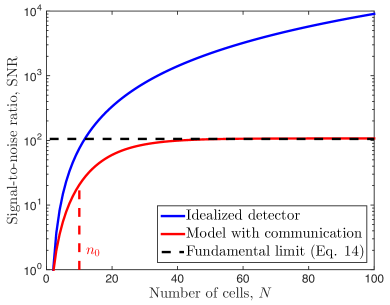
Figure 2: Precision of gradient sensing with temporal integration. Signal-to-noise ratio (SNR) vs. number of cells $N$ is shown for the idealized detector (Eqn. 2 with prefactor $1/\pi$) and for our model with communication (Eqs. 5, 6, 10, and 13). Whereas the SNR for the idealized detector increases indefinitely, the SNR for the model with communication saturates for $N\gg n_{0}$. The saturation level is bounded from above by the fundamental limit, Eqn. 14. As shown, the bound is reached in the high-gain regime $\alpha/a^{3}\mu=\beta/\nu=100$, where intrinsic noise is negligible. Other parameters are $a=10\ \mu$m, $\bar{c}_{N}=1$ nM, $g=1$ nM/mm, $D=50\ \mu$m²/s, $\mu=\nu=1$ s^-1, $n_{0}=\sqrt{\gamma/\nu}=10$, and the integration time scale is $T=10$ s.

I.3 Fundamental limit to sensory precision

The saturating value of the SNR is obtained in the limit of large $N$. In this limit, and when communication is strong ($\gamma\gg\nu$), the kernel (Eqn. 6) reduces to $K(n,n_{0})\approx e^{-n/n_{0}}/n_{0}$ us_unpublished . Here $n_{0}\equiv\sqrt{\gamma/\nu}$ sets the lengthscale of the kernel and therefore sets the number of neighboring cells with which the edge cell effectively communicates. The limit $\gamma\gg\nu$ and our assumption $T\gg\tau_{2}=1/\nu$ imply our third timescale assumption, $T\gg\tau_{3}\equiv 1/\gamma$, i.e. that the integration time is longer than the timescale of messenger exchange from cell to cell. Inserting the expression for $K(n,n_{0})$ into Eqn. 5, and approximating the sum as an integral in the large $N$ limit, the mean becomes $\bar{\Delta}_{N}\approx(\alpha\beta/\mu\nu)(\bar{c}_{N}-\bar{c}_{N-n_{0}})=\alpha\beta n_{0}ag/\mu\nu$. Inserting $K(n,n_{0})$ into Eqn. 13 results in products of the exponential with the $1/|n-n^{\prime}|$ dependence of the bound receptor power spectrum (Eqn. 10), leading to sums of the type $\sum_{j}e^{-j}/j$, which we evaluate in Appendix B. The result is

$$\frac{1}{{\rm SNR}} =\left(\frac{\delta\Delta_{N}}{\bar{\Delta}_{N}}\right)^{2}\gtrsim\frac{c_{\rm eff}}{\pi(n_{0}ag)^{2}aDT},\;{\rm where}$$ (14)

$$c_{\rm eff} \equiv\bar{c}_{N}+\frac{\log n_{0}}{2n_{0}}(\bar{c}_{N-n_{0}/2}-2\bar{c}_{N}),$$ (15)

and $T\gg\{\tau_{1},\tau_{2},\tau_{3}\}$. Eqn. 14 is fundamental in the sense that it does not depend on the details of the internal sensory mechanism. Rather, it only depends on the properties of the external signal ($c,g,D$), the physical dimensions ($a$), and the fact that information is integrated ($T$) and communicated ($n_{0}$) by the cells. The inequality reflects the fact that the righthand side contains additional positive terms arising from the finite number of bound receptors and intracellular molecules (see Appendix B). These terms represent intrinsic noise and can in principle be made arbitrarily small by increasing the gain factors $\alpha/a^{3}\mu$ and $\beta/\nu$, which dictate the internal molecule numbers. What remains in Eqn. 14 is the communicated extrinsic noise, which arises unavoidably from the diffusive fluctuations in the numbers of the ligand molecules being detected. Eqn. 14 is shown to bound the exact SNR in Fig. 2.

Comparing Eqn. 14 to the expression for the idealized detector (Eqn. 2), we see that the expressions are very similar but contain two important differences. First, whereas Eqn. 2 decreases indefinitely with $N$, Eqn. 14 remains bounded by $n_{0}$ for large $N$ (see Fig. 2). Evidently, a very large detector is limited in its precision to that of a smaller detector with effective size $n_{0}$. This limitation reflects the fact that reliable communication is restricted to a finite lengthscale. Importantly, Eqn. 14 demonstrates that this noise is present independently of the number of intrinsic signaling molecules in the communication channel. Thus the fundamental sensory limit is affected not only by the measurement process (as in BP theory), but also unavoidably by the communication process.

The second important difference is that Eqn. 2 depends on $\bar{c}_{N}$, whereas Eqn. 14 depends on the effective concentration $c_{\rm eff}$, defined in Eqn. 15. $c_{\rm eff}$ is a sum of the concentration measured by the local species, by the global species, and the covariance between them, respectively. The local species measures the concentration only within its local vicinity, $\bar{c}_{N}$. However, the global species effectively measures the concentration in the vicinity of $n_{0}$ cells. This fact reduces the noise associated with this term (and the covariance term) by the factor of $n_{0}$ in the denominator of Eqn. 15. Because intercellular molecular exchange also competes with extracellular molecular diffusion, not all of the measurements made by these $n_{0}$ cells are independent. Therefore, the reduction is tempered by the $\log n_{0}$ factor in the numerator of Eqn. 15. This log arises from the interaction of the $e^{-n}$ exchange kernel with the $1/|n-n^{\prime}|$ diffusion kernel (Appendix B). The net result is that, because of the correlations imposed by externals diffusion, the number of independent measurements grows sublinearly with the system size. Nonetheless, it does grow, and, correspondingly, in Eqn. 15 the measurement noise in the global species decreases with the communication lengthscale $n_{0}$. Crucially, this means that Eqn. 14 is dominated by the measurement noise of the local species, i.e. the first term in Eqn. 15.

In deriving the precision of gradient sensing, we have also derived the precision of concentration sensing by communicating cells. Specifically, by focusing only on the global species terms, and following the steps leading to Eqn. 14, we get

$$\left(\frac{\delta y_{N}}{\bar{y}_{N}}\right)^{2}\gtrsim\frac{1}{2\pi a_{\rm eff}DTc_{\rm eff}},$$ (16)

where $a_{\rm eff}\equiv an_{0}/\log n_{0}$ and $c_{\rm eff}\equiv\bar{c}_{N-n_{0}}^{2}/\bar{c}_{N-n_{0}/2}$. This expression has the same form as the BP limit, $(\delta c/\bar{c})^{2}\sim 1/(aDT\bar{c})$. Indeed, in the absence of a gradient, $\bar{c}_{n}=\bar{c}_{N}$ is constant, and $c_{\rm eff}\to\bar{c}_{N}$. Importantly, however, the effect of communication remains present in $a_{\rm eff}$: messenger exchange expands the effective detection lengthscale by a factor $n_{0}$, while ligand diffusion once again tempers the expansion by $\log n_{0}$. The net result is that communication reduces error by increasing the effective detector size, $a_{\rm eff}>a$.

I.4 Optimal sensing strategy

In the previous section, we saw that the limit to the precision of multicellular gradient sensing is dominated by the measurement noise of the local species in the edge cell (Eqns. 14 and 15). In contrast, the measurement noise of the global species is reduced by the intercellular communication. This finding raises an interesting question: could the total noise be further reduced if the local species were also exchanged between cells? To explore this possibility, we extend the model in Eqns. 3 and I.2 to allow for exchange of the local species at rate $\gamma_{x}$, and we take $\gamma\to\gamma_{y}>\gamma_{x}$ for the global species. An immediate consequence of this modification is that the signal becomes $\bar{\Delta}_{N}\approx\alpha\beta(n_{y}-n_{x})ag/\mu\nu$, where $n_{x}\equiv\gamma_{x}/\nu$ and $n_{y}=\gamma_{y}/\nu$. Thus the signal is reduced by local exchange, since increasing $\gamma_{x}$ decreases the difference $n_{y}-n_{x}$. This is because the signal is defined by the difference between the global and local readouts, and allowing for the local species exchange makes the two readouts less different. We thus anticipate that any useful local exchange rate will satisfy $\gamma_{x}\ll\gamma_{y}$ to maintain sufficiently high signal. In this limit, we find that Eqn. 15 remains dominated by the first term, even as local exchange reduces this term according to $c_{N}\to\bar{c}_{N}(\log n_{x})/2n_{x}$. Eqn. 14 then becomes

$${\rm SNR}\lesssim\frac{2\pi(ag)^{2}aDT}{\bar{c}_{N}}\frac{(n_{y}-n_{x})^{2}n_{x}}{\log n_{x}}.$$ (17)

For large $n_{y}$, this expression has a maximum as a function of $n_{x}$. The maximum arises due to a fundamental tradeoff: exchange of the local species reduces the signal, but it also reduces the dominant local measurement noise.

The optimal value $n_{x}^{*}$ depends on $n_{y}$. Experiments in epithelial cells suggest that the communication lengthscale $n_{y}$ is on the order of a few to ten cells us_unpublished . In this range, we find the optimum numerically from the exact SNR, which comes from straightforwardly generalizing Eqn. 13 (Appendix C). Fig. 3 shows that $n_{x}^{*}$ is about half of $n_{y}$ for one specific set of parameters, leading to an optimal exchange rate ratio of $\gamma_{x}^{*}/\gamma_{y}=(n_{x}^{*}/n_{y})^{2}\approx 25\%$. While the exact optimal ratio depends on the relative strengths of different noises, and hence on the gains (see Fig. 4 in Appendix C), the main finding is robust: a multicellular system should exchange both antagonistic messenger molecules, one at a fraction of the rate of the other. We call this strategy regional excitation–global inhibition (REGI). Fig. 3 shows that the enhancement over the one-messenger LEGI strategy can be substantial. For example, with $n_{y}=10$ cells, the SNR is optimally enhanced by a factor of $5$. With $n_{y}=15$, the enhancement is almost $8$-fold.

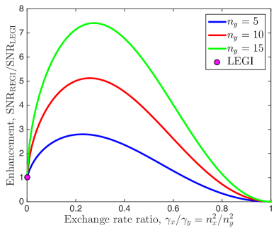
Figure 3: Regional excitation–global inhibition (REGI). Signal-to-noise ratio (SNR) is enhanced by allowing both messengers to be exchanged between cells. The optimal enhancement over LEGI is substantial and occurs because exchange of the local species reduces measurement noise, but also reduces the signal. Parameters are as in Fig. 2, but with $N=100$, $\alpha/a^{3}\mu=\beta/\nu=5$ and several values of $n_{y}\equiv\sqrt{\gamma_{y}/\nu}$ as indicated.

II Discussion

Cellular sensing of spatially inhomogeneous concentrations is a fundamental biological computation, involved in a variety of processes in the development and behavior of living systems. Like binocular vision and stereophonic sound processing, it is a process where the sensing is done by an array of spatially distributed sensors. Thus the accuracy of sensing is limited in part by the physical properties of the biological machinery that brings together the many spatially distributed measurements. Understanding these limits is a difficult problem.

Here we solved this problem in the case where the communication is diffusive, and one-dimensional distributed measurements are used to calculate external concentration gradients within the LEGI paradigm. We allowed for temporal integration, extending the results of Ref. us_unpublished . Some of the features of the gradient sensing limit we derived (Eqn. 14), such as the unbounded increase of the SNR with the diffusion coefficient of the ligand or with the integration time, carry over from the Berg-Purcell theory of gradient sensing Endres2008 , which does not account for communication. However, our most important finding is that, in contrast to the BP theory, the growth of the sensor array beyond a certain size stops increasing the SNR. The effect is independent of the intrinsic noise in the communication system and thus represents a truly fundamental limitation of diffusive communication for distributed sensing. In particular, it holds for multicellular systems, as well as for large individual cells. Although we derived the limit for a linear signal profile, we anticipate that the limit for a nonlinear profile will be similar, Eqn. 14, but with a different effective concentration $c_{\rm eff}$. It remains to be seen if similar limits hold when the sensors are arranged in two- or three-dimensional structures, or when concentration information propagates super-diffusively, as is possible in wave-based or Turing-type models of polarization establishment Jilkine:2011fy . Additionally, it will be important to relax various assumptions of the model, such as allowing for saturation of receptors or limiting the total number of messengers, and coupling the model to the motility apparatus to investigate how the improved sensory precision affects downstream functions.

Our results illustrate two important features of temporal averaging by distributed sensors. First, our derivation naturally reveals which timescales are relevant in this process, namely receptor equilibration ($\tau_{1}=\mu^{-1}+K/4\pi\sigma D$), messenger turnover ($\tau_{2}=1/\nu$), and messenger exchange ($\tau_{3}=1/\gamma$). In principle, these timescales could have depended on system-level properties, such as the system size ($N$) or the communication length ($n_{0}$). Surprisingly, instead they depend only on single-cell properties, meaning that efficient temporal averaging is not slowed down by increasing the number of sensors. Second, our results reveal the effects of over-counting due to correlations between external and internal diffusion. In both gradient sensing (Eqns. 14 and 15) and concentration sensing (Eqn. 16), we see that the noise reduction afforded by communication-based averaging is tempered by a factor $\log n_{0}$. This log is not a mathematical curiosity. Rather, it reflects the fact that not all measurements communicated to a cell by its neighbors are independent since the signal molecules also diffuse externally. Coupling external diffusion with internal exchange introduces correlations among measurements, which reduces the benefit of internal averaging.

Another central prediction is that the gradient sensing is improved by a system with two messengers, exchanged at different rates. We call this mechanism regional excitation–global inhibition (REGI), a generalization of the standard local excitation–global inhibition (LEGI) model. Optimality of REGI follows directly from the interplay between the ligand stochasticity and the communication constraints. Therefore, REGI has not been identified as an optimal strategy in previous studies that neglected either of these two effects. However, evidence for REGI may already exist in large gradient-sensing cells, where activated receptor complexes, which diffuse in the membrane at a rate $\sim$$10$$-$$100$ times slower than similar cytosolic molecules kholodenko , may act as the regional messengers.

REGI emerged from maximizing the SNR in our system, which revealed the optimal rate ratio $\gamma_{x}/\gamma_{y}$. Maximization of the SNR also implies that the optimal value of $\gamma_{y}$ (or $n_{y}$) is infinity, since the SNR grows indefinitely with $n_{y}$ (see Fig. 3). Infinite $n_{y}$ corresponds to averaging over as large a distance as possible. Such a strategy is only optimal here because the concentration profile is linear, with constant gradient $g$. In contrast, more physical nonlinear profiles (e.g. exponential, power-law, randomly varying, or profiles with extrema) have spatially varying $g$. In these cases, if the size of the group of cells is larger than the correlation length of $g$, then an infinite $n_{y}$ would average out the signal together with the noise, which would reduce the SNR. In contrast, a finite $n_{y}$ would allow a subset of cells to detect the local gradient in their vicinity, which is an essential task in morphological processes such as tissue branching and collective migration.

REGI can be interpreted as performing a spatial derivative. Specifically, the two-lobed filter $K(n,n_{x})-K(n,n_{y})$ reports the difference in concentrations measured over distances $n_{x}$ and $n_{y}$ near a given detector, and the values $n_{x}$ and $n_{y}$ depend on the properties of the environment. Thus REGI is similar to the temporal differentiation in E. coli chemotaxis. Indeed, the temporal filter of the E. coli sensory module is also two-lobed, with the short and long timescales set by ligand statistics and rotational diffusion, respectively Berg:2004wy . Thus, for both spatial and temporal filtering, the choice of the two optimal length- or timescales is determined by matching the filter to the statistical properties of the signal and the noise Wiener , which is understood well for E. coli Berg:2004wy .

Interpreting the REGI model as a spatiotemporal filter suggests experiments that would identify if a certain biological system employs this mechanism. Such experiments would involve concentration profiles that differ substantially from steady-state linear gradients. For example, subjecting cells to a concentration profile with a spatially localized maximum would allow one to measure both $\gamma_{x}$ and $\gamma_{y}$ by observing the response of cells near the concentration peak as a function of the peak width. Alternatively, one can subject cells to a spatiotemporally localized concentration pulse and observe if a response a certain distance away from the pulse exhibits the signs of only inhibition (LEGI, one messenger), or inhibition and excitation on different scales (REGI, two messengers). Understanding fundamental sensory limits for diffusive communication in gradient sensing opens up possibilities to propose and analyze these and other related experiments.

Appendix A Power spectrum of the bound receptor number

The dynamics of receptor binding are given in Fourier space by the first two lines of Eqn. 7,

$$-i\omega\tilde{\delta c} =-Dk^{2}\tilde{\delta c}+i\omega\sum_{n}\tilde{\delta r}_{n}e^{i\vec{k}\cdot\vec{x}_{n}},$$ (18)

$$-i\omega\tilde{\delta r}_{n} =\alpha\hat{\delta c}(\vec{x}_{n},\omega)-\mu\tilde{\delta r}_{n}+\alpha\bar{c}_{n}\tilde{\delta F}_{n},$$ (19)

where

$$\hat{\delta c}(\vec{x},\omega)\equiv\int d^{3}k\,(2\pi)^{-3}\tilde{\delta c}(\vec{k},\omega)e^{-i\vec{k}\cdot\vec{x}}.$$ (20)

We solve Eqn. 18 for $\tilde{\delta c}$ and, using Eqn. 20, insert it into Eqn. 19 to obtain

$$\{\mu-i\omega[1+\alpha\Sigma(\omega)]\}\tilde{\delta r}_{n}-i\omega\alpha\sum_{n^{\prime}\neq n}V(|\vec{x}_{n}-\vec{x}_{n^{\prime}}|,\omega)\tilde{\delta r}_{n^{\prime}}=\alpha\bar{c}_{n}\tilde{\delta F}_{n},$$ (21)

where

$$\Sigma(\omega) \equiv\int\frac{d^{3}k}{(2\pi)^{3}}\frac{1}{Dk^{2}-i\omega}=\frac{1}{2\pi^{2}}\int_{0}^{\infty}dk\frac{k^{2}}{Dk^{2}-i\omega},\quad\mbox{and}$$ (22)

$$V(x,\omega) \equiv\int\frac{d^{3}k}{(2\pi)^{3}}\frac{e^{-i\vec{k}\cdot\vec{x}}}{Dk^{2}-i\omega}=\frac{1}{2\pi^{2}x}\int_{0}^{\infty}dk\frac{k\sin(kx)}{Dk^{2}-i\omega}$$ (23)

are the “self-energy” and “interaction potential” between cells mediated by diffusion, respectively Bialek2005 . The simplifications in Eqns. 22 and 23 come from writing the volume element $d^{3}k=k^{2}\sin\theta\,dk\,d\theta\,d\phi$ in spherical coordinates aligned with $\vec{x}$, such that $\vec{k}\cdot\vec{x}=kx\cos\theta$.

We are interested in the low-frequency limits of $\Sigma(\omega)$ and $V(x,\omega)$. $V(x,0)=1/(4\pi Dx)$ is finite, whereas $\Sigma(0)$ diverges. The divergence stems from the delta functions in the dynamical equations, which model the cells as point sources. As in Bialek2005 , we regularize the divergence by introducing a cutoff $\Lambda\sim\pi/a$ at large $k$ to account for the fact that cells have finite extent $a$, making $\Sigma(0)\sim(2\pi^{2})^{-1}\int_{0}^{\Lambda}dk/D=1/(2\pi aD)$. This models cells as spheres of diameter $a$, but the exact shape of the cell will not be important for the limits we take. These expressions allow us to write Eqn. 21 as

$$\sum_{n^{\prime}=1}^{N}L_{nn^{\prime}}\tilde{\delta r}_{n^{\prime}}=\frac{\alpha\bar{c}_{n}}{\mu}\left(1+i\omega\tau_{1}\right)\tilde{\delta F}_{n},$$ (24)

where

$$\tau_{1} \equiv \frac{1}{\mu}+\frac{\alpha/\mu}{2\pi aD},$$ (25)

$$L_{nn^{\prime}} \equiv \delta_{nn^{\prime}}+\frac{z(1-\delta_{nn^{\prime}})}{|n-n^{\prime}|},$$ (26)

$$z \equiv -i\omega\frac{\alpha/\mu}{4\pi aD}.$$ (27)

In writing Eqn. 24, we have assumed that $\omega\tau_{1}$ is small. This assumption is valid for integration times $T=2\pi/\omega$ much longer than $\tau_{1}$. The quantity $\tau_{1}$ is the receptor equilibration time: it is the time it takes for a signal molecule to unbind from the receptors and diffuse away from the cell into the bulk Agmon1990 . Its first term $\mu^{-1}$ is the intrinsic receptor unbinding time, and its second term $K/4\pi\sigma D$ (where $K=\alpha/\mu$ is the equilibrium constant and $\sigma=a/2$ is the cell radius) accounts for rebinding events that occur before the molecule diffuses away from the cell completely Kaizu2014 . Either term can dominate: the first term dominates if the intrinsic association rate $\alpha$ is much smaller than the diffusion-limited association rate $4\pi\sigma D$, because then the molecule rarely rebinds. Conversely, the second term dominates if $\alpha$ is much larger than $4\pi\sigma D$, because then rebinding is frequent, and comprises most of the escape time. We see from Eqns. 25 and 27 that $|z|<\omega\tau_{1}$; therefore, we also treat $z$ as a small parameter.

Solving Eqn. 24 for $\tilde{\delta r}_{n}$ requires inverting the matrix $L_{nn^{\prime}}$. This matrix is a Toeplitz matrix (a matrix with constant diagonals), which has a known inversion algorithm Zohar1969 . Since $L_{nn^{\prime}}$ is also symmetric, it is completely specified by its first row $[1\ \rho_{1}\ \rho_{2}\ \dots\ \rho_{N-1}]$. The inversion is performed recursively as follows. First one introduces $N-1$ scalars $h_{1}$, $h_{2}$, $\dots$, $h_{N-1}$ and $N-1$ column vectors $\vec{q}^{(1)}$, $\vec{q}^{(2)}$, $\dots$, $\vec{q}^{(N-1)}$. These are initialized as

$$h_{1}=1-(\rho_{1})^{2},\qquad\vec{q}^{(1)}=[-\rho_{1}],$$ (28)

and updated as

$$h_{k+1}=h_{k}-\frac{(\zeta_{k})^{2}}{h_{k}},\qquad\vec{q}^{(k+1)}=\left[\begin{matrix}\vec{q}^{(k)}-\zeta_{k}\hat{\vec{q}}^{(k)}/h_{k}\\ -\zeta_{k}/h_{k}\\ \end{matrix}\right],$$ (29)

where $\zeta_{k}\equiv\rho_{k+1}+\sum_{\ell=1}^{k}\rho_{\ell}\hat{q}^{(k)}_{\ell}$, and $\hat{\vec{q}}$ is $\vec{q}$ with the elements in reverse order. Then the inverse is written in terms of the final quantities $h_{N-1}\equiv H$ and $\vec{q}^{(N-1)}\equiv\vec{Q}$. The upper left element is

$$L^{-1}_{11}=1/H,$$ (30)

the rest of the first row and column are

$$L^{-1}_{i+1,1}=L^{-1}_{1,i+1}=Q_{i}/H\qquad(1\leq i\leq N-1),$$ (31)

and the diagonals are calculated recursively from the first row and column as

$$L^{-1}_{i+1,j+1}=L^{-1}_{ij}+(Q_{i}Q_{j}-\hat{Q}_{i}\hat{Q}_{j})/H\qquad(1\leq\{i,j\}\leq N-1).$$ (32)

We now apply this algorithm to Eqn. 26, keeping only terms up to first order in the small quantity $z$. From Eqn. 26 we have $\rho_{j}=z/j$. The initial values are

$$h_{1}=1-z^{2}\approx 1,\qquad\vec{q}^{(1)}=[-z].$$ (33)

Using $\zeta_{1}=z/2+(z)(z)\approx z/2$, the first recursive step gives

$$h_{2}=1-\frac{(z/2)^{2}}{1}\approx 1,\qquad\vec{q}^{(2)}=\left[\begin{matrix}-z-(z/2)(-z)/(1)\\ -(z/2)/(1)\\ \end{matrix}\right]\approx\left[\begin{matrix}-z\\ -z/2\\ \end{matrix}\right].$$ (34)

Continuing the recursion establishes the general formulas

$$h_{k}=1,\qquad\vec{q}^{(k)}_{j}=-z/j\qquad(j\leq k),$$ (35)

from which we extract the final values,

$$H=1,\qquad Q_{j}=-z/j.$$ (36)

These values immediately provide the first row and column of the inverse according to Eqns. 30 and 31. Then noting that the second term on the right hand side of Eqn. 32 is second order in $z$, that equation implies that the diagonals of the inverse are constant. We therefore have the inverse to first order in $z$,

$$L^{-1}_{nn^{\prime}}=\delta_{nn^{\prime}}-\frac{z(1-\delta_{nn^{\prime}})}{|n-n^{\prime}|}.$$ (37)

The inverse allows us to solve Eqn. 24 for $\tilde{\delta r}_{n}$,

$$\tilde{\delta r}_{n}=\sum_{n^{\prime}=1}^{N}G_{nn^{\prime}}\tilde{\delta F}_{n^{\prime}}$$ (38)

where

$$G_{nn^{\prime}}(\omega)=\frac{\alpha}{\mu}\left(1+i\omega\tau_{1}\right)L^{-1}_{nn^{\prime}}\bar{c}_{n^{\prime}}=\begin{cases}\frac{\alpha\bar{c}_{n}}{\mu}\left[1+i\frac{\omega}{\mu}\left(1+\frac{\alpha}{2\pi aD}\right)\right]&n^{\prime}=n,\\ \frac{\alpha^{2}\omega\bar{c}_{n^{\prime}}}{4\pi aD\mu^{2}|n-n^{\prime}|}\left[i-\frac{\omega}{\mu}\left(1+\frac{\alpha}{2\pi aD}\right)\right]&n^{\prime}\neq n,\end{cases}$$ (39)

is the generalized susceptibility. The fluctuation-dissipation theorem then gives the power spectrum,

$$S^{rr}_{nn^{\prime}}(\omega)=\frac{2}{\omega}{\rm Im}[G_{nn^{\prime}}(\omega)]=\frac{2\alpha\bar{c}_{n^{\prime}}}{\mu^{2}}\begin{cases}\left(1+\frac{\alpha}{2\pi aD}\right)&n^{\prime}=n,\\ \frac{\alpha}{4\pi aD}\frac{1}{|n-n^{\prime}|}&n^{\prime}\neq n,\end{cases}$$ (40)

as in Eqn. 10.

Appendix B SNR in the many-cell, strong-communication limit

The variance of the readout is given by Eqn. 13,

$$(\delta\Delta_{N})^{2}=\frac{\beta^{2}}{\nu^{2}}\left[\frac{S^{rr}_{NN}(0)}{T}+\sum_{n,n^{\prime}=1}^{N}K_{N-n}K_{N-n^{\prime}}\frac{S^{rr}_{nn^{\prime}}(0)}{T}-2\sum_{n=1}^{N}K_{N-n}\frac{S^{rr}_{Nn}(0)}{T}\right]+\frac{2}{\nu T}\left(\bar{x}_{N}+K_{0}\bar{y}_{N}\right),$$ (41)

where $\bar{x}_{N}=\alpha\beta\bar{c}_{N}/\mu\nu$ and $\bar{y}_{N}=\alpha\beta\sum_{n=0}^{N-1}K_{n}\bar{c}_{N-n}/\mu\nu$. In the limit of many cells ($N\gg 1$) and strong communication ($\gamma\gg\nu$), the kernel takes the approximate form

$$K_{n}\approx\frac{1}{n_{0}}e^{-n/n_{0}},$$ (42)

where $n_{0}\equiv\sqrt{\gamma/\nu}\gg 1$ is the communication lengthscale. Using Eqns. 40 and 42, we evaluate Eqn. 41 term by term.

The first, fourth, and fifth terms in Eqn. 41 are straightforward,

$$\frac{\beta^{2}}{\nu^{2}}\frac{S^{rr}_{NN}(0)}{T} = \frac{2}{\mu T}\frac{\alpha\beta^{2}}{\mu\nu^{2}}\bar{c}_{N}+\frac{1}{\pi aDT}\frac{\alpha^{2}\beta^{2}}{\mu^{2}\nu^{2}}\bar{c}_{N},$$ (43)

$$\frac{2}{\nu T}\bar{x}_{N} = \frac{2}{\nu T}\frac{\alpha\beta}{\mu\nu}\bar{c}_{N},$$ (44)

$$\frac{2}{\nu T}K_{0}\bar{y}_{N} = \frac{2}{\nu T}\frac{\alpha\beta}{\mu\nu}\frac{\bar{c}_{N-n_{0}}}{n_{0}}.$$ (45)

In the last equation we use the limit of large $N$ to approximate the sum in $\bar{y}_{N}$ as an integral,

$$\sum_{n=0}^{N-1}K_{n}\bar{c}_{N-n}\approx\int_{0}^{\infty}dn\ \frac{1}{n_{0}}e^{-n/n_{0}}(\bar{c}_{N}-nag)=\bar{c}_{N}-n_{0}ag=\bar{c}_{N-n_{0}}.$$ (46)

The third term in Eqn. 41 we split in two,

$$-2\frac{\beta^{2}}{\nu^{2}}\sum_{n=1}^{N}K_{N-n}\frac{S^{rr}_{Nn}(0)}{T}=-2\frac{\beta^{2}}{\nu^{2}}\left[K_{0}\frac{S^{rr}_{NN}(0)}{T}+\sum_{n=1}^{N-1}K_{N-n}\frac{S^{rr}_{Nn}(0)}{T}\right].$$ (47)

The first of these is like Eqn. 43

$$-2\frac{\beta^{2}}{\nu^{2}}K_{0}\frac{S^{rr}_{NN}(0)}{T}=-\frac{4}{\mu T}\frac{\alpha\beta^{2}}{\mu\nu^{2}}\frac{\bar{c}_{N}}{n_{0}}-\frac{2}{\pi aDT}\frac{\alpha^{2}\beta^{2}}{\mu^{2}\nu^{2}}\frac{\bar{c}_{N}}{n_{0}}.$$ (48)

The second evaluates to

$$-2\frac{\beta^{2}}{\nu^{2}}\sum_{n=1}^{N-1}K_{N-n}\frac{S^{rr}_{Nn}(0)}{T} = -2\frac{\beta^{2}}{\nu^{2}}\sum_{n=1}^{N-1}\frac{1}{n_{0}}e^{-(N-n)/n_{0}}\frac{2\alpha}{\mu^{2}T}[\bar{c}_{N}-(N-n)ag]\frac{\alpha}{4\pi aD}\frac{1}{N-n}$$ (49)

$$= -\frac{1}{\pi aDT}\frac{\alpha^{2}\beta^{2}}{\mu^{2}\nu^{2}}\left[\frac{\bar{c}_{N}}{n_{0}}\sum_{j=1}^{N-1}\frac{e^{-j/n_{0}}}{j}-\frac{ag}{n_{0}}\sum_{j=1}^{N-1}e^{-j/n_{0}}\right]$$ (50)

$$\approx -\frac{1}{\pi aDT}\frac{\alpha^{2}\beta^{2}}{\mu^{2}\nu^{2}}\left[\frac{\bar{c}_{N}}{n_{0}}\log n_{0}-ag\right],$$ (51)

where the last step again uses the integral approximation for large $N$. In particular, we have written

$$\sum_{j=1}^{N-1}\frac{e^{-j/n_{0}}}{j}\approx\int_{1}^{\infty}dj\ \frac{e^{-j/n_{0}}}{j}=\Gamma(0,1/n_{0})\approx\log n_{0}-\gamma_{e}\approx\log n_{0},$$ (52)

using the small-argument limit of the upper incomplete Gamma function. The last step assumes that $\log n_{0}$ is much larger than the Euler-Mascheroni constant $\gamma_{e}\approx 0.577$. Numerically, we have checked that Eqn. 52 is valid for $5\lesssim n_{0}\ll N$. Altogether, the third term in Eqn. 41 is then

$$-2\frac{\beta^{2}}{\nu^{2}}\sum_{n=1}^{N}K_{N-n}\frac{S^{rr}_{Nn}(0)}{T} = -\frac{4}{\mu T}\frac{\alpha\beta^{2}}{\mu\nu^{2}}\frac{\bar{c}_{N}}{n_{0}}-\frac{2}{\pi aDT}\frac{\alpha^{2}\beta^{2}}{\mu^{2}\nu^{2}}\left[\frac{\bar{c}_{N}}{n_{0}}+\frac{\bar{c}_{N}}{2n_{0}}\log n_{0}-\frac{ag}{2}\right]$$ (53)

$$\approx -\frac{4}{\mu T}\frac{\alpha\beta^{2}}{\mu\nu^{2}}\frac{\bar{c}_{N}}{n_{0}}-\frac{2}{\pi aDT}\frac{\alpha^{2}\beta^{2}}{\mu^{2}\nu^{2}}\frac{\log n_{0}}{2n_{0}}\bar{c}_{N},$$ (54)

where the second step uses $\bar{c}_{N}-agn_{0}/2=\bar{c}_{N-n_{0}/2}<\bar{c}_{N}$ and assumes $\log n_{0}\gg 2$.

The second term in Eqn. 41 we also split in two,

$$\frac{\beta^{2}}{\nu^{2}}\sum_{n,n^{\prime}=1}^{N}K_{N-n}K_{N-n^{\prime}}\frac{S^{rr}_{nn^{\prime}}(0)}{T}=\frac{\beta^{2}}{\nu^{2}}\left[\sum_{n=1}^{N}K_{N-n}^{2}\frac{S^{rr}_{nn}(0)}{T}+\sum_{n=1}^{N}\sum_{n^{\prime}\neq n}K_{N-n}K_{N-n^{\prime}}\frac{S^{rr}_{nn^{\prime}}(0)}{T}\right].$$ (55)

The first of these is straightforward to evaluate with the integral approximation in Eqn. 46,

$$\frac{\beta^{2}}{\nu^{2}}\sum_{n=1}^{N}K_{N-n}^{2}\frac{S^{rr}_{nn}(0)}{T} = \frac{\beta^{2}}{\nu^{2}}\sum_{j=0}^{N-1}\frac{1}{n_{0}^{2}}e^{-2j/n_{0}}\frac{2\alpha\bar{c}_{N-j}}{\mu^{2}T}\left(1+\frac{\alpha}{2\pi aD}\right)$$ (56)

$$\approx \frac{2}{\mu T}\frac{\alpha\beta^{2}}{\mu\nu^{2}}\frac{\bar{c}_{N-n_{0}/2}}{2n_{0}}+\frac{1}{\pi aDT}\frac{\alpha^{2}\beta^{2}}{\mu^{2}\nu^{2}}\frac{\bar{c}_{N-n_{0}/2}}{2n_{0}}.$$ (57)

The second can be evaluated in two parts,

$$\frac{\beta^{2}}{\nu^{2}}\sum_{n=1}^{N}\sum_{n^{\prime}\neq n}K_{N-n}K_{N-n^{\prime}}\frac{S^{rr}_{nn^{\prime}}(0)}{T}=\frac{1}{2\pi aDT}\frac{\alpha^{2}\beta^{2}}{\mu^{2}\nu^{2}}\Bigg{[}\frac{\bar{c}_{N}}{n_{0}^{2}}\underbrace{\sum_{j=0}^{N-1}\sum_{j^{\prime}\neq j}\frac{e^{-(j+j^{\prime})/n_{0}}}{|j-j^{\prime}|}}_{A}-\frac{ag}{n_{0}^{2}}\underbrace{\sum_{j=0}^{N-1}\sum_{j^{\prime}\neq j}\frac{j^{\prime}e^{-(j+j^{\prime})/n_{0}}}{|j-j^{\prime}|}}_{B}\Bigg{]}.$$ (58)

Notice that $B=-\partial_{u}A/2$, where $u\equiv 1/n_{0}$, so that we only need to evaluate $A$. We split $A$ into two equal components,

$$A = \sum_{j=0}^{N-1}\sum_{j^{\prime}=0}^{j-1}\frac{e^{-(j+j^{\prime})/n_{0}}}{j-j^{\prime}}+\sum_{j=0}^{N-1}\sum_{j^{\prime}=j+1}^{N-1}\frac{e^{-(j+j^{\prime})/n_{0}}}{j^{\prime}-j}$$ (59)

$$= 2\sum_{j=0}^{N-1}\sum_{j^{\prime}=0}^{j-1}\frac{e^{-(j+j^{\prime})/n_{0}}}{j-j^{\prime}},$$ (60)

and rewrite it in terms of $k=j+j^{\prime}$ and $\ell=j-j^{\prime}$,

$$A=2\sum_{\ell=1}^{N-1}\sum_{k=\ell,\ell+2,\ell+4,\dots}^{2(N-1)-\ell}\frac{e^{-k/n_{0}}}{\ell}.$$ (61)

We approximate with integrals for large $N$, accounting for the fact that $k$ has support on only half of the integers in its range,

$$A \approx 2\int_{1}^{N}d\ell\ \frac{1}{2}\int_{\ell}^{2(N-1)-\ell}dk\ \frac{e^{-k/n_{0}}}{\ell}$$ (62)

$$= n_{0}\int_{1}^{N}d\ell\ \frac{e^{-\ell/n_{0}}}{\ell}-n_{0}e^{-2N}\int_{1}^{N}d\ell\ \frac{e^{\ell/n_{0}}}{\ell}.$$ (63)

The first integral is approximately $\log n_{0}$ by Eqn. 52. The second integral evaluates to ${\rm Ei}(N/n_{0})-{\rm Ei}(1/n_{0})$, where Ei is the exponential integral function, whose large- and small-argument limits are ${\rm Ei}(N/n_{0})\approx e^{N/n_{0}}/(N/n_{0})$ and ${\rm Ei}(1/n_{0})\approx-\log n_{0}$, respectively. Thus, the second term in Eqn. 63 vanishes exponentially with $N$, and we have

$$A = n_{0}\log n_{0},$$ (64)

$$B = \frac{n_{0}^{2}}{2}(1+\log n_{0})\approx\frac{n_{0}^{2}}{2}\log n_{0},$$ (65)

making the term in brackets in Eqn. 58 equal to $(\bar{c}_{N}-agn_{0}/2)(\log n_{0})/n_{0}=(\bar{c}_{N-n_{0}/2}\log n_{0})/n_{0}$. Altogether, the second term in Eqn. 41 is then

$$\frac{\beta^{2}}{\nu^{2}}\sum_{n,n^{\prime}=1}^{N}K_{N-n}K_{N-n^{\prime}}\frac{S^{rr}_{nn^{\prime}}(0)}{T} = \frac{2}{\mu T}\frac{\alpha\beta^{2}}{\mu\nu^{2}}\frac{\bar{c}_{N-n_{0}/2}}{2n_{0}}+\frac{1}{\pi aDT}\frac{\alpha^{2}\beta^{2}}{\mu^{2}\nu^{2}}\left[\frac{\bar{c}_{N-n_{0}/2}}{2n_{0}}+\frac{\log n_{0}}{2n_{0}}\bar{c}_{N-n_{0}/2}\right]$$ (66)

$$\approx \frac{2}{\mu T}\frac{\alpha\beta^{2}}{\mu\nu^{2}}\frac{\bar{c}_{N-n_{0}/2}}{2n_{0}}+\frac{1}{\pi aDT}\frac{\alpha^{2}\beta^{2}}{\mu^{2}\nu^{2}}\frac{\log n_{0}}{2n_{0}}\bar{c}_{N-n_{0}/2},$$ (67)

where the second step assumes $\log n_{0}\gg 1$.

Finally, collecting the terms in Eqns. 43-45, 54, and 67, the variance in Eqn. 41 becomes

$$(\delta\Delta_{N})^{2}=\left(\frac{\alpha\beta}{a^{3}\mu\nu}\right)^{2}\Bigg{[} \underbrace{\frac{a^{2}}{\pi DT}\left(\bar{c}_{N}+\frac{\log n_{0}}{2n_{0}}\bar{c}_{N-n_{0}/2}-2\frac{\log n_{0}}{2n_{0}}\bar{c}_{N}\right)a^{3}}_{{\rm{\bf Extrinsic}\ noise\ from\ }c,\ {\rm propagated\ to\ }x\ {\rm and\ }y}$$

$$+\underbrace{\frac{2}{\mu T}\frac{a^{3}\mu}{\alpha}\left(\bar{c}_{N}+\frac{\bar{c}_{N-n_{0}/2}}{2n_{0}}-2\frac{\bar{c}_{N}}{n_{0}}\right)a^{3}}_{{\rm{\bf Intrinsic}\ noise\ in\ }r,\ {\rm propagated\ to\ }x\ {\rm and\ }y}$$

$$+\underbrace{\frac{2}{\nu T}\frac{a^{3}\mu}{\alpha}\frac{\nu}{\beta}\left(\bar{c}_{N}\right)a^{3}}_{{\rm{\bf Intrinsic}\ noise\ in\ }x}+\underbrace{\frac{2}{\nu T}\frac{a^{3}\mu}{\alpha}\frac{\nu}{\beta}\left(\frac{\bar{c}_{N-n_{0}}}{n_{0}}\right)a^{3}}_{{\rm{\bf Intrinsic}\ noise\ in\ }y}\Bigg{]}.$$ (68)

The last line contains the intrinsic noise from $x_{N}$ and $y_{N}$. For example, the first term in this line is $(\delta x_{N})^{2}=(2/\nu T)(\alpha\beta\bar{c}_{N}/\mu\nu)=2\bar{x}_{N}/\nu T$; the relative noise $(\delta x_{N}/\bar{x}_{N})^{2}=2/\nu T\bar{x}_{N}$ then decreases with the number of molecules $\bar{x}_{N}\times\nu T$ that are turned over in time $T$, as expected for intrinsic counting noise. The second term in this line is for $y$ and is similar, except that since the global species is exchanged over roughly $n_{0}$ cells, more molecules are counted and the noise is reduced by a factor $n_{0}$. The second line contains the intrinsic noise in $r$, propagated to $x$ and $y$. The third line contains the noise in $c$, propagated to $x$ and $y$, which we deem extrinsic, since it originates in the environment and is not under direct control of the cells.

Importantly, the intrinsic noise terms in Eqn. B are reducible by increasing the numbers of receptors and local and global species molecules. These molecule numbers are set by the gain factors $\bar{r}_{N}/a^{3}\bar{c}_{N}=\alpha/a^{3}\mu$ and $\bar{x}_{N}/\bar{r}_{N}=\beta/\nu$, and indeed, we see that the second and third lines in Eqn. B vanish as the gain factors grow large. In this limit we are left with only the lower bound set by the extrinsic noise,

$$(\delta\Delta_{N})^{2}\geq\left(\frac{\alpha\beta}{\mu\nu}\right)^{2}\frac{1}{\pi aDT}\left(\bar{c}_{N}+\frac{\log n_{0}}{2n_{0}}\bar{c}_{N-n_{0}/2}-2\frac{\log n_{0}}{2n_{0}}\bar{c}_{N}\right).$$ (69)

Dividing by the square of the mean $\bar{\Delta}_{N}=\alpha\beta n_{0}ag/\mu\nu$ produces Eqns. 14 and 15.

Appendix C Exact SNR for regional excitation–global inhibition (REGI)

In the REGI strategy, both messengers X and Y are exchanged between cells, at rates $\gamma_{x}$ and $\gamma_{y}$, respectively. This results in a straightforward generalization of the expression for the signal-to-noise ratio (SNR). Specifically, the mean becomes (compare to Eqns. 5 and 6 in the main text)

$$\bar{\Delta}_{N}=\frac{\alpha\beta}{\mu\nu}\left(\sum_{n=0}^{N-1}K^{x}_{n}\bar{c}_{N-n}-\sum_{n=0}^{N-1}K^{y}_{n}\bar{c}_{N-n}\right),$$ (70)

where now there are two communication kernels,

$$K^{x}_{n}=\frac{\sum_{j=0}^{N-n-1}{N-n-1+j\choose 2j}(\nu/\gamma_{x})^{j}}{\sum_{\ell=0}^{N-1}{N+\ell\choose 2\ell+1}(\nu/\gamma_{x})^{\ell}},$$ (71)

$$K^{y}_{n}=\frac{\sum_{j=0}^{N-n-1}{N-n-1+j\choose 2j}(\nu/\gamma_{y})^{j}}{\sum_{\ell=0}^{N-1}{N+\ell\choose 2\ell+1}(\nu/\gamma_{y})^{\ell}}.$$ (72)

The variance becomes (compare to Eqn. 13)

$$(\delta\Delta_{N})^{2}=\frac{\beta^{2}}{\nu^{2}}\left[\sum_{nn^{\prime}}\left(K^{x}_{N-n}K^{x}_{N-n^{\prime}}+K^{y}_{N-n}K^{y}_{N-n^{\prime}}-2K^{x}_{N-n}K^{y}_{N-n^{\prime}}\right)\frac{S^{rr}_{nn^{\prime}}(0)}{T}\right]+\frac{2}{\nu T}\left(K^{x}_{0}\bar{x}_{N}+K^{y}_{0}\bar{y}_{N}\right),$$ (73)

where the bound receptor power spectrum $S^{rr}_{nn^{\prime}}(\omega)$ remains the same as in Eqn. 10 (or equivalently Eqn. 40). The SNR is then $(\bar{\Delta}_{N}/\delta\Delta_{N})^{2}$.

The SNR has a maximum as a function of the rate ratio $\gamma_{x}/\gamma_{y}$. The location of the maximum $\gamma_{x}^{*}/\gamma_{y}$ must lie between $0$ and $1$. At $\gamma_{x}/\gamma_{y}=0$, the X messenger is not exchanged, and we recover the SNR of the local excitation–global inhibition (LEGI) strategy, which is a limiting case of REGI. At $\gamma_{x}/\gamma_{y}=1$, there is no difference between X and Y, and the signal (and therefore the SNR) is $0$. The exact location of $\gamma_{x}^{*}/\gamma_{y}$ depends on factors that are specific to the system, e.g. the concentration profile $\bar{c}_{n}$, the environmental and system parameters, and the measurement location ($n=1$ vs. $n=N$).

We illustrate the dependence of $\gamma_{x}^{*}/\gamma_{y}$ on particular system parameters, namely the gain factors $\alpha/a^{3}\mu$ and $\beta/\nu$. For this, Fig. 4 shows the dependence on SNR on $\gamma_{x}/\gamma_{y}$ as we vary the gain factors $\alpha/a^{3}\mu$ (A) and $\beta/\nu$ (B). In both cases, we see that the optimal rate ratio $\gamma_{x}^{*}/\gamma_{y}$ increases with increasing gain. This is because increasing either gain factor increases the number of internal messenger molecules. With more molecules, the system can afford to increase $\gamma_{x}$ while maintaining the same difference in molecule number $\Delta_{N}$ in the $N$th cell. The increase in $\gamma_{x}$ enhances the spatial averaging by the X messenger, and thus reduces the noise in the estimate of $\bar{c}_{N}$. Therefore, we see in Fig. 4 that the maximal SNR occurs at a higher $\gamma_{x}^{*}$ value as either gain is increased.

Figure 4: Dependence of the optimal exchange rate ratio on system parameters in the regional excitation–global inhibition (REGI) strategy. The signal-to-noise ratio (SNR) has a maximum at a particular rate ratio $\gamma_{x}^{*}/\gamma_{y}$, which increases as a function of either gain factor, (A) $\alpha/a^{3}\mu$, or (B) $\beta/\nu$. Parameters are $a=10\ \mu$m, $\bar{c}_{N}=1$ nM, $g=1$ nM/mm, $D=50\ \mu$m²/s, $T=10$ s, $\mu=\nu=1$ s^-1, $N=100$, and $n_{y}=\sqrt{\gamma/\nu}=10$. In A, $\beta/\nu=5$, and $\alpha/a^{3}\mu$ is varied as indicated. In B, $\alpha/a^{3}\mu=5$, and $\beta/\nu$ is varied as indicated.