Provably Correct Algorithms for Matrix Column Subset Selection with Selectively Sampled Data

Abstract

We consider the problem of matrix column subset selection, which selects a subset of columns from an input matrix such that the input can be well approximated by the span of the selected columns. Column subset selection has been applied to numerous real-world data applications such as population genetics summarization, electronic circuits testing and recommendation systems. In many applications the complete data matrix is unavailable and one needs to select representative columns by inspecting only a small portion of the input matrix. In this paper we propose the first provably correct column subset selection algorithms for partially observed data matrices. Our proposed algorithms exhibit different merits and limitations in terms of statistical accuracy, computational efficiency, sample complexity and sampling schemes, which provides a nice exploration of the tradeoff between these desired properties for column subset selection. The proposed methods employ the idea of feedback driven sampling and are inspired by several sampling schemes previously introduced for low-rank matrix approximation tasks (Drineas et al., 2008; Frieze et al., 2004; Deshpande and Vempala, 2006; Krishnamurthy and Singh, 2014). Our analysis shows that, under the assumption that the input data matrix has incoherent rows but possibly coherent columns, all algorithms provably converge to the best low-rank approximation of the original data as number of selected columns increases. Furthermore, two of the proposed algorithms enjoy a relative error bound, which is preferred for column subset selection and matrix approximation purposes. We also demonstrate through both theoretical and empirical analysis the power of feedback driven sampling compared to uniform random sampling on input matrices with highly correlated columns.

Keywords: Column subset selection, active learning, leverage scores

1 Introduction

Given a matrix $\mathbf{M}\in\mathbb{R}^{n_{1}\times n_{2}}$, the column subset selection problem aims to find $s$ exact columns in $\mathbf{M}$ that capture as much of $\mathbf{M}$ as possible. More specifically, we want to select $s$ columns of $\mathbf{M}$ to form a column sub-matrix $\mathbf{C}\in\mathbb{R}^{n_{1}\times s}$ to minimize the norm of the following residue

$$\min_{\mathbf{X}\in\mathbb{R}^{s\times n_{2}}}{\|\mathbf{M}-\mathbf{C}\mathbf{X}\|_{\xi}}=\|\mathbf{M}-\mathbf{C}\mathbf{C}^{\dagger}\mathbf{M}\|_{\xi},$$ (1)

where $\mathbf{C}^{\dagger}$ is the Moore-Penrose pseudoinverse of $\mathbf{C}$ and $\xi=2$ or $F$ denotes the spectral or Frobenius norm. In this paper we mainly focus on the Frobenius norm, as was the case in previous theoretical analysis for sampling based column subset selection algorithms (Drineas et al., 2008; Frieze et al., 2004; Deshpande and Vempala, 2006; Deshpande et al., 2006). To evaluate the performance of column subset selection, one compares the residue norm defined in Eq. (1) with $\|\mathbf{M}-\mathbf{M}_{k}\|_{\xi}$, where $\mathbf{M}_{k}$ is the best rank-$k$ approximation of $\mathbf{M}$. Usually the number of selected columns $s$ is larger than or equal to the target rank $k$. Two forms of error guarantee are common: additive error guarantee in Eq. (2) and relative error guarantee in Eq. (3), with $0<\epsilon<1$ and $c>1$ (ideally $c=1+\epsilon$).

$$\|\mathbf{M}-\mathbf{C}\mathbf{C}^{\dagger}\mathbf{M}\|_{\xi} \leq \|\mathbf{M}-\mathbf{M}_{k}\|_{\xi}+\epsilon\|\mathbf{M}\|_{F};$$ (2)

$$\|\mathbf{M}-\mathbf{C}\mathbf{C}^{\dagger}\mathbf{M}\|_{\xi} \leq c\|\mathbf{M}-\mathbf{M}_{k}\|_{\xi}.$$ (3)

In general, relative error bound is much more appreciated because $\|\mathbf{M}\|_{\xi}$ is usually large in practice, while $\|\mathbf{M}-\mathbf{M}_{k}\|_{2}$ is expected to be small when the goal is low-rank approximation. In addition, when $\mathbf{M}$ is an exact low-rank matrix Eq. (3) implies perfect reconstruction, while the error in Eq. (2) remains non-zero. The column subset selection problem can be considered as a form of unsupervised feature selection or prototype selection, which arises frequently in the analysis of large data sets. For example, column subset selection has been applied to various tasks such as summarizing population genetics, testing electronic circuits, recommendation systems, etc. Interested readers should refer to (Boutsidis et al., 2009; Balzano et al., 2010a) for further motivations.

Many methods have been proposed for the column subset selection problem (Chan, 1987; Gu and Eisenstat, 1996; Frieze et al., 2004; Deshpande et al., 2006; Drineas et al., 2008; Boutsidis et al., 2014). An excellent summarization of these methods and their theoretical guarantee is available in Table 1 in (Boutsidis et al., 2009). Most of these methods can be roughly categorized into two classes. One class of algorithms are based on rank-revealing QR (RRQR) decomposition (Chan, 1987; Gu and Eisenstat, 1996) and it has been shown in (Boutsidis et al., 2009) that RRQR is nearly optimal in terms of residue norm under the $s=k$ setting, that is, exact $k$ columns are selected to reconstruct an input matrix. On the other hand, sampling based methods (Frieze et al., 2004; Deshpande et al., 2006; Drineas et al., 2008) try to select columns by sampling from certain distributions over all columns of an input matrix. Extension of sampling based methods to general low-rank matrix approximation problems is also investigated (Cohen et al., 2015; Bhojanapalli et al., 2015). These algorithms are much faster than RRQR and achieves comparable performance if the sampling distribution is carefully selected and slight over-sampling (i.e., $s>k$) is allowed (Deshpande et al., 2006; Drineas et al., 2008). In (Boutsidis et al., 2009) sampling based and RRQR based algorithms are unified to arrive at an efficient column subset selection method that uses exactly $s=k$ columns and is nearly optimal.

Although the column subset selection problem with access to the full input matrix has been extensively studied, often in practice it is hard or even impossible to obtain the complete data. For example, for the genetic variation detection problem it could be expensive and time-consuming to obtain full DNA sequences of an entire population. Several heuristic algorithms have been proposed recently for column subset selection with missing data, including the Block OMP algorithm (Balzano et al., 2010a) and the group Lasso formulation explored in (Bien et al., 2010). Nevertheless, no theoretical guarantee or error bounds have been derived for these methods. The presence of missing data poses new challenges for column subset selection, as many well-established algorithms seem incapable of handling missing data in an elegant way. Below we identify a few key challenges that prevent application of previous theoretical results on column subset selection under the missing data setting:

• Coherent matrix design: most previous results on the completion or recovery of low rank matrices with incomplete data assume the underlying data matrix is incoherent (Recht, 2011; Candes and Plan, 2010; Keshavan et al., 2010), which intuitively assumes all rows and columns in the data matrix are weakly correlated. On the other hand, previous algorithms on column subset selection and matrix CUR decomposition spent most efforts on dealing with coherent matrices (Deshpande et al., 2006; Drineas et al., 2008; Boutsidis et al., 2009; Boutsidis and Woodruff, 2014). In fact, one can show that under standard incoherence assumptions of matrix completion algorithms a high-quality column subset can be obtained by sampling each column uniformly at random, which trivializes the problem (Xu et al., 2015). Such gap in problem assumptions renders column subset selection on incomplete coherent matrices particularly difficult. In this paper, we explore the possibility of a weaker incoherence assumption that bridges the gap. We present and discuss detailed assumptions considered in this paper in Sec. 1.1.

• Limitation of existing sampling schemes: previous matrix completion methods usually assume the observed data are sampled uniformly at random. However, in (Krishnamurthy and Singh, 2014) it is proved that uniform sampling (in fact any sampling scheme with apriori fixed sampling distribution) is not sufficient to complete a coherent matrix. Though in (Chen et al., 2013) a provably correct sampling scheme was proposed for any matrix based on statistical leverage scores, which is also the key ingredient of many previous column subset selection and matrix CUR decomposition algorithms (Drineas et al., 2008; Boutsidis et al., 2009; Boutsidis and Woodruff, 2014), it is very difficult to approximate the leverage scores of an incomplete coherent matrix. Common perturbation results on singular vector space (e.g., Wedin’s theorem) fail because closeness between two subspaces does not imply closeness in their leverage scores since the latter are defined in an infinity norm manner (see Section 2.1 for details).

• Limitation of zero filling: A straightforward algorithm for missing data column subset selection is to first fill all unobserved entries with zero and then properly scale the observed ones so that the completed matrix is consistent with the underlying data matrix in expectation (Achlioptas and McSherry, 2007; Achlioptas et al., 2013). Column subset selection algorithms designed for fully observed data could be applied afterwards on the zero-filled matrix. However, the zero filling procedure can change the underlying subspace of a matrix drastically (Balzano et al., 2010b) and usually leads to additive error bounds as in Eq. (2). To achieve stronger relative error bounds we need an algorithm that goes beyond the zero filling idea.

In this paper, we propose three column subset selection algorithms based on the idea of active sampling of the input matrix. In our algorithms, observed matrix entries are chosen sequentially and in a feedback-driven manner. We motivate this sampling setting from both practical and theoretical perspectives. In applications where each entry of a data matrix $\mathbf{M}$ represents results from an expensive or time-consuming experiment, it makes sense to carefully select which entry to query (experiment), possibly in a feedback-driven manner, so as to reduce experimental cost. For example, if $\mathbf{M}$ has drugs as its columns and targets (proteins) as its rows, it makes sense to cautiously select drug-target pairs for sequential experimental study in order to find important drugs/targets with typical drug-target interactions. From a theoretical perspective, we show in Section 7.1 that no passive sampling scheme is capable of achieving relative-error column subset selection with high probability, even if the column space of $\mathbf{M}$ is incoherent. Such results suggest that active/adaptive sampling is to some extent unavoidable, unless both row and column spaces of $\mathbf{M}$ are incoherent.

We also remark that the algorithms we consider make very few measurements of the input matrix, which differs from previous feedback-driven re-sampling methods in the theoretical computer science literature (e.g., (Wang and Zhang, 2013)) that requires access to the entire input matrix. Active sampling has been shown to outperform all passive schemes in several settings (cf. (Haupt et al., 2011; Kolar et al., 2011)), and furthermore it works for completion of matrices with incoherent rows/columns under which passive learning provably fails (Krishnamurthy and Singh, 2013, 2014). To the best of our knowledge, the algorithms proposed in this paper are the first column subset selection algorithms for coherent matrices that enjoy theoretical error guarantee with missing data, whether passive or active. Furthermore, two of our proposed methods achieve relative error bounds.

1.1 Assumptions

Completing/approximating partially observed low-rank matrices using a subset of columns requires certain assumptions on the input data matrix $\mathbf{M}$ (Candes and Plan, 2010; Chen et al., 2013; Recht, 2011; Xu et al., 2015). To see this, consider the extreme-case example where the input data matrix $\mathbf{M}$ consists of exactly one non-zero element (i.e., $\mathbf{M}_{ij}=1\{i=i^{*},j=j^{*}\}$ for some $i^{*}\in[n_{1}]$ and $j^{*}\in[n_{2}]$). In this case, the relative approximation quality $c=\|\mathbf{M}-\mathbf{C}\mathbf{C}^{\dagger}\mathbf{M}\|_{\xi}/\|\mathbf{M}-\mathbf{M}_{1}\|_{\xi}$ in Eq. (3) would be infinity if column $j^{*}$ is not selected in $\mathbf{C}$. In addition, it is clearly impossible to correctly identify $j^{*}$ using $o(n_{1}n_{2})$ observations even with active sampling strategies. Therefore, additional assumptions on $\mathbf{M}$ are required to provably approximate a partially observed matrix using column subsets.

In this work we consider the assumption that the top-$k$ column space of the input matrix $\mathbf{M}$ is incoherent (detailed mathematical definition given in Sec. 2.1), while placing no incoherence or spikiness assumptions on the actual columns, rows or the row space of $\mathbf{M}$. In addition to the necessity of incoherence assumptions for incomplete matrix approximation problems discussed above, we further motivate the “one-sided” incoherence assumption from two perspectives:

• Column subset selection with incomplete observation remains a non-trivial problem even if the column space is assumed to be incoherent. Due to the possible heterogeneity of the columns, naive methods such as column subsets sampled uniformly at random are in general bad approximations of the original data matrix $\mathbf{M}$. Existing column subset selection algorithms for fully-observed matrices also need to be majorly revised to accommodate missing matrix components.

• Compared to existing work on approximating low-rank incomplete matrices, our assumptions (one-sided incoherence) are arguably weaker. Xu et al. (2015) analyzed matrix CUR approximation of partially observed matrices, but assumed that both column and row spaces are incoherent; Krishnamurthy and Singh (2014) derived an adaptive sampling procedure to complete a low-rank matrix with only one-sided incoherence assumptions, but only achieved additive error bounds for noisy low-rank matrices.

• Finally, the one-sided incoherence assumption is reasonable in a number of practical scenarios. For example, in the application of drug-target interaction prediction, the one-sided incoherence assumption allows for highly specialized or diverse drugs while assuming some predictability between target protein responses.

1.2 Our contributions

The main contribution of this paper is three provably correct algorithms for column subset selection, which are inspired by existing work on column subset selection for fully-observed matrices, but only inspect a small portion of the input matrix. The sampling schemes for the proposed algorithms and their main merits and drawbacks are summarized below:

1. Norm sampling: The algorithm is simple and works for any input matrix with incoherent column subspace. However, it only achieves an additive error bound as in Eq. (2). It is also inferior than the other two proposed methods in terms of residue error on both synthetic and real-world data sets.

2. Iterative norm sampling: The iterative norm sampling algorithm enjoys relative error guarantees as in Eq. (3) at the expense of being much more complicated and computationally expensive. In addition, its correctness is only proved for low-rank matrices with incoherent column space corrupted with i.i.d. Gaussian noise.

3. Approximate leverage score sampling: The algorithm enjoys relative error guarantee for general (high-rank) input matrices with incoherent column space. However, it requires more over-sampling and its error bound is worse than the one for iterative norm sampling on noisy low-rank matrices. Moreover, to actually reconstruct the data matrix the approximate leverage score sampling scheme requires sampling a subset of both entire rows and columns, while both norm based algorithms only require sampling of some entire columns.

In summary, our proposed algorithms offer a rich, provably correct toolset for column subset selection with missing data. Furthermore, a comprehensive understanding of the design tradeoffs among statistical accuracy, computational efficiency, sample complexity, and sampling scheme, etc. is achieved by analyzing different aspects of the proposed methods. Our analysis could provide further insights into other matrix completion/approximation tasks on partially observed data.

We also perform comprehensive experimental study of column subset selection with missing data using the proposed algorithms as well as modifications of heuristic algorithms proposed recently (Balzano et al., 2010a; Bien et al., 2010) on synthetic matrices and two real-world applications: tagging Single Nucleotide Polymorphisms (tSNP) selection and column based image compression. Our empirical study verifies most of our theoretical results and reveals a few interesting observations that are previously unknown. For instance, though leverage score sampling is widely considered as the state-of-the-art for matrix CUR approximation and column subset selection, our experimental results show that under certain low-noise regimes (meaning that the input matrix is very close to low rank) iterative norm sampling is more preferred and achieves smaller error. These observations open new questions and suggest the need for new analysis in related fields, even for the fully observed case.

1.3 Notations

For any matrix $\mathbf{M}$ we use $\mathbf{M}^{(i)}$ to denote the $i$-th column of $\mathbf{M}$. Similarly, $\mathbf{M}_{(i)}$ denotes the $i$-th row of $\mathbf{M}$. All norms $\|\cdot\|$ are $\ell_{2}$ norms or the matrix spectral norm unless otherwise specified.

We assume the input matrix is of size $n_{1}\times n_{2}$, $n=\max(n_{1},n_{2})$. We further assume that $n_{1}\leq n_{2}$. We use $\boldsymbol{x}_{i}=\mathbf{M}^{(i)}\in\mathbb{R}^{n_{1}}$ to denote the $i$-th column of $\mathbf{M}$. Furthermore, for any column vector $\boldsymbol{x}_{i}\in\mathbb{R}^{n_{1}}$ and index subset $\Omega\subseteq[n_{1}]$, define the subsampled vector $\boldsymbol{x}_{i,\Omega}$ and the scaled subsampled vector $\mathcal{R}_{\Omega}(\boldsymbol{x}_{i})$ as

$$\boldsymbol{x}_{i,\Omega}=\boldsymbol{1}_{\Omega}\circ\boldsymbol{x}_{i},\quad\mathcal{R}_{\Omega}(\boldsymbol{x}_{i})=\frac{n_{1}}{|\Omega|}\boldsymbol{1}_{\Omega}\circ\boldsymbol{x}_{i},$$ (4)

where $\boldsymbol{1}_{\Omega}\in\mathbb{\{}0,1\}^{n_{1}}$ is the indicator vector of $\Omega$ and $\circ$ is the Hadamard product (entrywise product). We also generalize the definition in Eq. (4) to matrices by applying the same operator on each column.

We use $\|\mathbf{M}-\mathbf{C}\mathbf{C}^{\dagger}\mathbf{M}\|_{\xi}$ to denote the selection error and $\|\mathbf{M}-\mathbf{C}\mathbf{X}\|_{\xi}$ to denote the reconstruction error. The difference between the two types of error is that for selection error an algorithm is only required to output indices of the selected columns while for reconstruction error an algorithm needs to output both the selected columns $\mathbf{C}$ and the coefficient matrix $\mathbf{X}$ so that $\mathbf{C}\mathbf{X}$ is close to $\mathbf{M}$. We remark that the reconstruction error always upper bounds the selection error due to Eq. (1). On the other hand, there is no simple procedure to compute $\mathbf{C}^{\dagger}\mathbf{M}$ when $\mathbf{M}$ is not fully observed.

1.4 Outline of the paper

The paper is organized as follows: in Section 2 we provide background knowledge and review several concepts that are important to our analysis. We then present main results of the paper, the three proposed algorithms and their theoretical guarantees in Section 3. Proofs for main results given in Section 3 are sketched in Section 4 and some technical lemmas and complete proof details are deferred to the appendix. In Section 5 we briefly describe previously proposed heuristic based algorithm for column subset selection with missing data and their implementation details. Experimental results are presented in Section 6 and we discuss several aspects including the limitation of passive sampling and time complexity of proposed algorithms in Section 7.

2 Preliminaries

This section provides necessary background knowledge for the analysis in this paper. We first review the concept of coherence, which plays an important row in sampling based matrix algorithms. We then summarize three matrix sampling schemes proposed in previous literature.

2.1 Subspace and vector incoherence

Incoherence plays a crucial role in various matrix completion and approximation tasks (Recht, 2011; Krishnamurthy and Singh, 2014; Candes and Plan, 2010; Keshavan et al., 2010). For any matrix $\mathbf{M}\in\mathbb{R}^{n_{1}\times n_{2}}$ of rank $k$, singular value decomposition yields $\mathbf{M}=\mathbf{U}\mathbf{\Sigma}\mathbf{V}^{\top}$, where $\mathbf{U}\in\mathbb{R}^{n_{1}\times k}$ and $\mathbf{V}\in\mathbb{R}^{n_{2}\times k}$ have orthonormal columns. Let $\mathcal{U}=\mathrm{span}(\mathbf{U})$ and $\mathcal{V}=\mathrm{span}(\mathbf{V})$ be the column and row space of $\mathbf{M}$. The column space coherence is defined as

$$\mu(\mathcal{U}):=\frac{n_{1}}{k}\max_{i=1}^{n_{1}}{\|\mathbf{U}^{\top}\boldsymbol{e}_{i}\|_{2}^{2}}=\frac{n_{1}}{k}\max_{i=1}^{n_{1}}{\|\mathbf{U}_{(i)}\|_{2}^{2}}.$$ (5)

Note that $\mu(\mathcal{U})$ is always between 1 and $n_{1}/k$. Similarly, the row space coherence is defined as

$$\mu(\mathcal{V}):=\frac{n_{2}}{k}\max_{i=1}^{n_{2}}{\|\mathbf{V}^{\top}\boldsymbol{e}_{i}\|_{2}^{2}}=\frac{n_{2}}{k}\max_{i=1}^{n_{2}}{\|\mathbf{V}_{(i)}\|_{2}^{2}}.$$ (6)

In this paper we also make use of incoherence level of vectors, which previously appeared in (Balzano et al., 2010b; Krishnamurthy and Singh, 2013, 2014). For a column vector $\boldsymbol{x}\in\mathbb{R}^{n_{1}}$, its incoherence is defined as

$$\mu(\boldsymbol{x}):=\frac{n_{1}\|\boldsymbol{x}\|_{\infty}^{2}}{\|\boldsymbol{x}\|_{2}^{2}}.$$ (7)

It is an easy observation that if $\boldsymbol{x}$ lies in the subspace $\mathcal{U}$ then $\mu(\boldsymbol{x})\leq k\mu(\mathcal{U})$. In this paper we adopt incoherence assumptions on the column space $\mathcal{U}$, which subsequently yields incoherent row vectors $\boldsymbol{x}_{i}$. No incoherence assumption on the row space $\mathcal{V}$ or row vectors $\mathbf{M}_{(i)}$ is made.

2.2 Matrix sampling schemes

Norm sampling: Norm sampling for column subset selection was proposed in (Frieze et al., 2004) and has found applications in a number of matrix computation tasks, e.g., approximate matrix multiplication (Drineas et al., 2006a) and low-rank or compressed matrix approximation (Drineas et al., 2006c, b). The idea is to sample each column with probability proportional to its squared $\ell_{2}$ norm, i.e., $\Pr[i\in C]\propto\|\mathbf{M}^{(i)}\|_{2}^{2}$ for $i\in\{1,2,\cdots,n_{2}\}$. These types of algorithms usually come with an additive error bound on their approximation performance.

Volume sampling: For volume sampling (Deshpande et al., 2006), a subset of columns $C$ is picked with probability proportional to the volume of the simplex spanned by columns in $C$. That is, $\Pr[C]\propto\mathrm{vol}(\Delta(C))$ where $\Delta(C)$ is the simplex spanned by $\{\mathbf{M}^{(C(1))},\cdots,\mathbf{M}^{(C(k))}\}$. Computationally efficient volume sampling algorithms exist (Deshpande and Rademacher, 2010; Anari et al., 2016). These methods are based on the computation of characteristic polynomials of the projected data matrix (Deshpande and Rademacher, 2010) or an MCMC sampling procedure (Anari et al., 2016). Under the partially observed setting, both approaches are difficult to apply. For the characteristic polynomials approach, one has to estimate the characteristic polynomial and essentially the least singular value of the target matrix $\mathbf{M}$ up to relative error bounds. This is not possible unless the matrix is very well-conditioned, which violates the setting that $\mathbf{M}$ is approximately low-rank. For the MCMC sampling procedure, it was shown in (Anari et al., 2016) that $O(kn_{2})$ iterations are needed for the sampling Markov chain to mix. As each sampling iteration requires observing one entire column, performing $O(kn_{2})$ iterations essentially requires observing $O(kn_{2})$ columns, i.e., the entire matrix $\mathbf{M}$. On the other hand, an iterative norm sampling procedure is known to perform approximate volume sampling and therefore enjoys multiplicative approximation bounds for column subset selection (Deshpande and Vempala, 2006). In this paper we generalize the iterative norm sampling scheme to the partially observed setting and demonstrate similar multiplicative approximation error guarantees.

Leverage score sampling: The leverage score sampling scheme was introduced in (Drineas et al., 2008) to get relative error bounds for CUR matrix approximation and has later been applied to coherent matrix completion (Chen et al., 2013). For each row $i\in\{1,\cdots,n_{1}\}$ and column $j\in\{1,\cdots,n_{2}\}$ define $\mu_{i}:=\frac{n_{1}}{k}\|\mathbf{U}^{\top}\boldsymbol{e}_{i}\|_{2}^{2}$ and $\nu_{j}:=\frac{n_{2}}{k}\|\mathbf{V}^{\top}\boldsymbol{e}_{j}\|_{2}^{2}$ to be their unnormalized leverage scores, where $\mathbf{U}\in\mathbb{R}^{n_{1}\times k}$ and $\mathbf{V}\in\mathbb{R}^{n_{2}\times k}$ are the top-k left and right singular vectors of an input matrix $\mathbf{M}$. It was shown in (Drineas et al., 2008) that if rows and columns are sampled with probability proportional to their leverage scores then a relative error guarantee is possible for matrix CUR approximation and column subset selection.

3 Column subset selection via active sampling

Table 1: Summary of theoretical guarantees of proposed algorithms. $s$ denotes the number of selected columns and $m$ denotes the expected number of observed matrix entries. Dependency on failure probability $\delta$ and other poly-logarithmic dependency is omitted. $\mathcal{U}$ represents the column space of $\mathbf{A}$.

	Error type	Error bound	$s$	$m$	Assumptions
Norm	$\|\mathbf{M}-\mathbf{C}\mathbf{C}^{\dagger}\mathbf{M}\|_{F}$	$\|\mathbf{M}-\mathbf{M}_{k}\|_{F}+\epsilon\|\mathbf{M}\|_{F}$	$\Omega(k/\epsilon^{2})$	$\widetilde{\Omega}(\mu_{1}n)$	$\max_{i=1}^{n_{2}}\mu(\mathbf{M}_{(i)})\leq\mu_{1}$
	$\|\mathbf{M}-\mathbf{C}\mathbf{X}\|_{F}$	$\|\mathbf{M}-\mathbf{M}_{k}\|_{F}+2\epsilon\|\mathbf{M}\|_{F}$	$\Omega(k/\epsilon^{2})$	$\widetilde{\Omega}(k\mu_{1}n/\epsilon^{4})$	same as above
Iter. norm	$\|\mathbf{M}-\mathbf{C}\mathbf{C}^{\dagger}\mathbf{M}\|_{F}$	$\sqrt{2.5^{k}(k+1)!}\|\mathbf{M}-\mathbf{M}_{k}\|_{F}$	$k$	$\widetilde{\Omega}(k^{2}\mu_{0}n)$	$\mathbf{M}=\mathbf{A}+\mathbf{R}$; $\mu(\mathcal{U})\leq\mu_{0}$
	$\|\mathbf{M}-\mathbf{C}\mathbf{C}^{\dagger}\mathbf{M}\|_{F}$	$\sqrt{1+3\epsilon}\|\mathbf{M}-\mathbf{M}_{k}\|_{F}$	$\Theta(k^{2}\log k+k/\epsilon)$	$\widetilde{\Omega}\left(\frac{k\mu_{0}n}{\epsilon}\left(k+\frac{1}{\epsilon}\right)\right)$	same as above
	$\|\mathbf{M}-\mathbf{C}\mathbf{X}\|_{F}$	$\sqrt{1+3\epsilon}\|\mathbf{M}-\mathbf{M}_{k}\|_{F}$	$\Theta(k^{2}\log k+k/\epsilon)$	$\widetilde{\Omega}\left(\frac{k\mu_{0}n}{\epsilon}\left(k+\frac{1}{\epsilon}\right)\right)$	same as above
Lev. score	$\|\mathbf{M}-\mathbf{C}\mathbf{C}^{\dagger}\mathbf{M}\|_{F}$	$3(1+\epsilon)\|\mathbf{M}-\mathbf{M}_{k}\|_{F}$	$\Omega(k^{2}/\epsilon^{2})$	$\Omega(k^{2}\mu_{0}n/\epsilon^{2})$	$\mu(\mathcal{U})\leq\mu_{0}$

In this section we propose three column subset selection algorithms that only observe a small portion of an input matrix. All algorithms employ the idea of active sampling to handle matrices with coherent rows. While Algorithm 1 achieves an additive reconstruction error guarantee for any matrix, Algorithm 2 achieves a relative-error reconstruction guarantee when the input matrix has certain structure. Finally, Algorithm 3 achieves a relative-error selection error bound for any general input matrix at the expense of slower error rate and more sampled columns. Table 1 summarizes the main theoretical guarantees for the proposed algorithms.

3.1 $\ell_{2}$ norm sampling

Algorithm 1 Active norm sampling for column subset selection with missing data

1:Input: size of column subset $s$, expected number of samples per column $m_{1}$ and $m_{2}$.

2:Norm estimation: For each column $i$, sample each index in $\Omega_{1,i}\subseteq[n_{1}]$ i.i.d. from $\mathrm{Bernoulli}(m_{1}/n_{1})$. observe $\boldsymbol{x}_{i,\Omega_{1,i}}$ and compute $\hat{c}_{i}=\frac{n_{1}}{m_{1}}\|\boldsymbol{x}_{i,\Omega_{1,i}}\|_{2}^{2}$. Define $\hat{f}=\sum_{i}{\hat{c}_{i}}$.

3:Column subset selection: Set $\mathbf{C}=\mathbf{0}\in\mathbb{R}^{n_{1}\times s}$.

• For $t\in[s]$: sample $i_{t}\in[n_{2}]$ such that $\Pr[i_{t}=j]=\hat{c}_{j}/\hat{f}$. Observe $\mathbf{M}^{(i_{t})}$ in full and set $\mathbf{C}^{(t)}=\mathbf{M}^{(i_{t})}$.

4:Matrix approximation: Set $\widehat{\mathbf{M}}=\mathbf{0}\in\mathbb{R}^{n_{1}\times n_{2}}$.

• For each column $\boldsymbol{x}_{i}$, sample each index in $\Omega_{2,i}\subseteq[n_{1}]$ i.i.d. from $\mathrm{Bernoulli}(m_{2,i}/n_{1})$, where $m_{2,i}=m_{2}n_{2}\hat{c}_{i}/\hat{f}$; observe $\boldsymbol{x}_{i,\Omega_{2,i}}$.

• Update: $\widehat{\mathbf{M}}=\widehat{\mathbf{M}}+(\mathcal{R}_{\Omega_{2,i}}(\boldsymbol{x}_{i}))\boldsymbol{e}_{i}^{\top}$.

5:Output: selected columns $\mathbf{C}$ and coefficient matrix ${\mathbf{X}}=\mathbf{C}^{\dagger}\widehat{\mathbf{M}}$.

We first present an active norm sampling algorithm (Algorithm 1) for column subset selection under the missing data setting. The algorithm is inspired by the norm sampling work for column subset selection by Frieze et al. (Frieze et al., 2004) and the low-rank matrix approximation work by Krishnamurthy and Singh (Krishnamurthy and Singh, 2014).

The first step of Algorithm 1 is to estimate the $\ell_{2}$ norm for each column by uniform subsampling. Afterwards, $s$ columns of $\mathbf{M}$ are selected independently with probability proportional to their $\ell_{2}$ norms. Finally, the algorithm constructs a sparse approximation of the input matrix by sampling each matrix entry with probability proportional to the square of the corresponding column’s norm and then a $\mathbf{C}\mathbf{X}$ approximation is obtained.

When the input matrix $\mathbf{M}$ has incoherent columns, the selection error as well as $\mathbf{C}\mathbf{X}$ reconstruction error can be bounded as in Theorem 9.

Theorem 1

Suppose $\max_{i=1}^{n_{2}}{\mu(\boldsymbol{x}_{i})}\leq\mu_{1}$ for some positive constant $\mu_{1}$. Let $\mathbf{C}$ and $\mathbf{X}$ be the output of Algorithm 1. Denote $\mathbf{M}_{k}$ as the best rank-$k$ approximation of $\mathbf{M}$. Fix $\delta=\delta_{1}+\delta_{2}+\delta_{3}>0$. With probability at least $1-\delta$, we have

$$\|\mathbf{M}-\mathbf{C}\mathbf{C}^{\dagger}\mathbf{M}\|_{F}\leq\|\mathbf{M}-\mathbf{M}_{k}\|_{F}+\epsilon\|\mathbf{M}\|_{F}$$ (8)

provided that $s=\Omega(k\epsilon^{-2}/\delta_{2})$, $m_{1}=\Omega(\mu_{1}\log(n/\delta_{1}))$. Furthermore, if $m_{2}=\Omega(\mu_{1}s\log^{2}(n/\delta_{3})/(\delta_{2}\epsilon^{2}))$ then with probability $\geq 1-\delta$ we have the following bound on reconstruction error:

$$\|\mathbf{M}-\mathbf{C}{\mathbf{X}}\|_{F}\leq\|\mathbf{M}-\mathbf{M}_{k}\|_{F}+2\epsilon\|\mathbf{M}\|_{F}.$$ (9)

As a remark, Theorem 9 shows that one can achieve $\epsilon$ additive reconstruction error using Algorithm 1 with expected sample complexity (omitting dependency on $\delta$)

$$\Omega\left(\mu_{1}n_{2}\log(n)+\frac{kn_{1}}{\epsilon^{2}}+\frac{k\mu_{1}n_{2}\log^{2}(n)}{\epsilon^{4}}\right)=\Omega(k\mu_{1}\epsilon^{-4}n\log^{2}n).$$

3.2 Iterative norm sampling

Algorithm 2 Active iterative norm sampling for column subset selection for data corrupted by Gaussian noise

1:Input: target rank $k<\min(n_{1},n_{2})$, error tolerance parameter $\epsilon$, $\delta$ and expected number of samples per column $m$.

2:Entrywise sampling: For each column $i$, sample each index in an index set $\Omega_{i}\subseteq[n_{1}]$ i.i.d. from $\mathrm{Bernoulli}(m/n_{1})$. Observe $\boldsymbol{x}_{i,\Omega_{i}}$.

3:Approximate volume sampling: Set $C=\mathcal{U}=\emptyset$. Let $\mathbf{U}$ be an orthonormal basis of $\mathcal{U}$.

4:for $t=1,2,\cdots,k$ do

5:     For $i\in\{1,\cdots,n_{2}\}$, compute $\hat{c}_{i}^{(t)}=\frac{n_{1}}{m}\|\boldsymbol{x}_{i,\Omega_{i}}-\mathbf{U}_{\Omega_{i}}(\mathbf{U}_{\Omega_{i}}^{\top}\mathbf{U}_{\Omega_{i}})^{-1}\mathbf{U}_{\Omega_{i}}^{\top}\boldsymbol{x}_{i,\Omega_{i}}\|_{2}^{2}$.

6:     Set $\hat{f}^{(t)}=\sum_{i=1}^{n_{2}}\hat{c}_{i}^{(t)}$.

7:     Select a column $i_{t}$ at random, with probability $\Pr[i_{t}=j]=\hat{p}_{j}^{(t)}=\hat{c}_{j}^{(t)}/\hat{f}^{(t)}$.

8:     Observe $\mathbf{M}^{(i_{t})}$ in full and update: $C\leftarrow C\cup\{i_{t}\}$, $\mathcal{U}\leftarrow\mathrm{span}(\mathcal{U},\{\mathbf{M}^{(i_{t})}\})$.

9:end for

10:Active norm sampling: set $T=(k+1)\log(k+1)$ and $s_{1}=s_{2}=\cdots=s_{T-1}=5k$, $s_{T}=10k/\epsilon\delta$; $S=\emptyset$, $\mathcal{S}=\emptyset$. Suppose $\mathbf{U}$ is an orthonormal basis of $\mathrm{span}(\mathcal{U},\mathcal{S})$.

11:for $t=1,2,\cdots,T$ do

12:     For $i\in\{1,\cdots,n_{2}\}$, compute $\hat{c}_{i}^{(t)}=\frac{n_{1}}{m}\|\boldsymbol{x}_{i,\Omega_{i}}-\mathbf{U}_{\Omega_{i}}(\mathbf{U}_{\Omega_{i}}^{\top}\mathbf{U}_{\Omega_{i}})^{-1}\mathbf{U}_{\Omega_{i}}^{\top}\boldsymbol{x}_{i,\Omega_{i}}\|_{2}^{2}$.

13:     Set $\hat{f}^{(t)}=\sum_{i=1}^{n_{2}}\hat{c}_{i}^{(t)}$.

14:     Select $s_{t}$ columns $S_{t}=(i_{1},\cdots,i_{s_{t}})$ independently at random, with probability $\Pr[j\in S_{t}]=\hat{q}_{j}^{(t)}=\hat{c}_{j}^{(t)}/\hat{f}^{(t)}$.

15:     Observe $\mathbf{M}^{(S_{t})}$ in full and update: $S\leftarrow S\cup S_{t}$, $\mathcal{S}\leftarrow\mathrm{span}(\mathcal{S},\{\mathbf{M}^{(S_{t})}\})$.

16:end for

17:Matrix approximation: $\widehat{\mathbf{M}}=\sum_{i=1}^{n_{2}}{\mathbf{U}(\mathbf{U}_{\Omega_{i}}^{\top}\mathbf{U}_{\Omega_{i}})^{-1}\mathbf{U}_{\Omega_{i}}\boldsymbol{x}_{i,\Omega_{i}}\boldsymbol{e}_{i}^{\top}}$, where $\mathbf{U}\in\mathbb{R}^{n_{1}\times(s+k)}$ is an orthonormal basis of $\mathrm{span}(\mathcal{U}_{0},\mathcal{U}_{1})$.

18:Output: selected column subsets $\mathbf{C}=(\mathbf{M}^{(C(1))},\cdots,\mathbf{M}^{(C(k))})\in\mathbb{R}^{n_{1}\times k}$, $\mathbf{S}=(\mathbf{M}^{(C)},\mathbf{M}^{(S_{1})},\cdots,\mathbf{M}^{(S_{T})})\in\mathbb{R}^{n_{1}\times s}$ where $s=k+s_{1}+\cdots+s_{T}$ and $\mathbf{X}=\mathbf{S}\mathbf{S}^{\dagger}\widehat{\mathbf{M}}$.

In this section we present Algorithm 2, another active sampling algorithm based on the idea of iterative norm sampling and approximate volume sampling introduced in (Deshpande and Vempala, 2006). Though Algorithm 2 is more complicated than Algorithm 1, it achieves a relative error bound on inputs that are noisy perturbation of some underlying low-rank matrix.

Algorithm 2 employs the idea of iterative norm sampling. That is, after selecting $l$ columns from $\mathbf{M}$, the next column (or next several columns depending on the error type) is sampled according to column norms of a projected matrix $\mathcal{P}_{\mathcal{C}^{\perp}}(\mathbf{M})$, where $\mathcal{C}$ is the subspace spanned by currently selected columns. It can be shown that iterative norm sampling serves as an approximation of volume sampling, a sampling scheme that is known to have relative error guarantees (Deshpande et al., 2006; Deshpande and Vempala, 2006).

Theorem 2 shows that when the input matrix $\mathbf{M}$ is the sum of an exact low rank matrix $\mathbf{A}$ and a stochastic noise matrix $\mathbf{R}$, then by selecting exact $k$ columns from $\mathbf{M}$ using iterative norm sampling one can upper bound the selection error $\|\mathbf{M}-\mathbf{C}\mathbf{C}^{\dagger}\mathbf{M}\|_{F}$ by the best rank-$k$ approximation error $\|\mathbf{M}-\mathbf{M}_{k}\|_{F}$ within a multiplicative factor that does not depend on the matrix size $n$. Such relative error guarantee is much stronger than the additive error bound provided in Theorem 9 as when $\mathbf{M}$ is exactly low rank the error is eliminated with high probability. In fact, when the input matrix $\mathbf{M}$ is exactly low rank the first phase of the proposed algorithm (Line 1 to Line 9 in Algorithm 2) resembles the adaptive sampling algorithm proposed in (Krishnamurthy and Singh, 2013, 2014) for matrix and tensor completion in the sense that at each iteration all columns falling exactly onto the span of already selected columns will have zero norm after projection and hence will never be sampled again. However, we are unable to generalize our algorithm to general full-rank inputs because it is difficult to bound the incoherence level of projected columns (and hence the projection accuracy itself later on) without a stochastic noise model. We present a new algorithm with slightly worse error bounds in Section 3.3 which can handle general high-rank inputs.

Though Eq. (10) is a relative error bound, the multiplicative factor scales exponentially with the intrinsic rank $k$, which is not completely satisfactory. As a remedy, we show that by slightly over-sampling the columns ($\Theta(k^{2}\log k+k/\epsilon\delta)$ instead of $k$ columns) the selection error as well as the $\mathbf{C}\mathbf{X}$ reconstruction error could be upper bounded by $\|\mathbf{M}-\mathbf{M}_{k}\|_{F}$ within only a $(1+3\epsilon)$ factor, which implies that the error bounds are nearly optimal when the number of selected columns $s$ is sufficiently large, for example, $s=\Omega(k^{2}\log k+k/\epsilon\delta)$.

Theorem 2

Fix $\delta>0$. Suppose $\mathbf{M}=\mathbf{A}+\mathbf{R}$, where $\mathbf{A}$ is a rank-$k$ deterministic matrix with incoherent column space (i.e., $\mu(\mathcal{U}(\mathbf{A}))\leq\mu_{0}$) and $\mathbf{R}$ is a random matrix with i.i.d. zero-mean Gaussian distributed entries. Suppose $k=O(n_{1}/\log(n_{2}/\delta))$. Let $\mathbf{C},\mathbf{S}$ and $\mathbf{X}$ be the output of Algorithm 2. Then the following holds:

1. If $m=\Omega(k^{2}\mu_{0}\log^{2}(n/\delta))$ then with probability $\geq 1-\delta$

   $$\|\mathbf{M}-\mathbf{C}\mathbf{C}^{\dagger}\mathbf{M}\|_{F}^{2}\leq\frac{2.5^{k}(k+1)!}{\delta}\|\mathbf{R}\|_{F}^{2}.$$ (10)

   The column subset size is $k$ and the corresponding sample complexity is $\Omega(k^{2}\mu_{0}n\log^{2}(n/\delta))$.

2. If $m=\Omega(\epsilon^{-1}s\mu_{0}\log^{2}(n/\delta))$ with $s=\Theta(k^{2}\log k+k/\epsilon\delta)$, then with probability $\geq 1-\delta$

   $$\|\mathbf{M}-\mathbf{S}\mathbf{S}^{\dagger}\mathbf{M}\|_{F}^{2}\leq\|\mathbf{M}-\mathbf{S}\mathbf{X}\|_{F}^{2}\leq(1+3\epsilon)\|\mathbf{R}\|_{F}^{2}.$$ (11)

   The column subset size is $\Theta(k^{2}\log k+k/\epsilon\delta)$ and the sample complexity is (omitting dependence on $\delta$)

   $$\Omega\left(\frac{k^{2}\mu_{0}n\log k\log^{2}(n)}{\epsilon}+\frac{k\mu_{0}n\log^{2}(n)}{\epsilon^{2}}\right).$$

3.3 Approximate leverage score sampling

Algorithm 3 Approximate leverage score sampling for column subset selection on general input matrices

1:Input: target rank $k$, size of column subset $s$, expected number of row samples $m$.

2:Leverage score estimation: Set $\mathcal{S}=\emptyset$.

• For each row $i$, with probability $m/n_{1}$ observe the row $\mathbf{M}_{(i)}$ in full and update $\mathcal{S}\leftarrow\mathrm{span}(\mathcal{S},\{\mathbf{M}_{(i)}\})$.

• Compute the first $k$ right singular vectors of $\mathcal{S}$ (denoted by $\mathbf{S}_{k}\in\mathcal{R}^{n_{2}\times k}$) and estimate the unnormalized row space leverage scores as $\tilde{l}_{j}=\|{\mathbf{S}_{k}}^{\top}\boldsymbol{e}_{j}\|_{2}^{2}$, $j\in\{1,2,\cdots,n_{1}\}$.

3:Column subset selection: Set $C=\emptyset$.

• For $t\in\{1,2,\cdots,s\}$ select a column $i_{t}\in[n_{2}]$ with probability $Pr[i_{t}=j]=\hat{p}_{j}=\tilde{l}_{j}/k$; update $C\leftarrow C\cup\{i_{t}\}$.

4:Output: the selected column indices $C\subseteq\{1,2,\cdots,n_{2}\}$ and actual columns $\mathbf{C}=(\mathbf{M}^{(C(1))},\cdots,\mathbf{M}^{(C(s))})$.

The third sampling-based column subset selection algorithm for partially observed matrices is presented in Algorithm 3. The proposed algorithm was based on the leverage score sampling scheme for matrix CUR approximation introduced in (Drineas et al., 2008). To compute the sampling distribution (i.e., leverage scores) from partially observed data, the algorithm subsamples a small number of rows from the input matrix and uses leverage scores of the row space of the subsampled matrix to form the sampling distribution. Note that we do not attempt to approximate leverage scores of the original input matrix directly; instead, we compute leverage scores of another matrix that is a good approximation of the original data. Such technique was also explored in (Drineas et al., 2012) to approximate statistical leverages in a fully observed setting. Afterwards, column sampling distribution is constructed using the estimated leverage scores and a subset of columns are selected according to the constructed sampling distribution.

We bound the selection error $\|\mathbf{M}-\mathbf{C}\mathbf{C}^{\dagger}\mathbf{M}\|_{F}$ of the approximate leverage score sampling algorithm in Theorem 3. Note that unlike Theorem 9 and 2, only selection error bound is provided since for deterministic full-rank input matrices it is challenging to approximately compute the projection of $\mathbf{M}$ onto $\mathrm{span}(\mathbf{C})$ because the projected vector may no longer be incoherent (this is in fact the reason why Theorem 2 holds only for low-rank matrices perturbed by Gaussian noise, and we believe similar conclusion should also hold for Algorithm 3 is the stronger assumption of Gaussian noise perturbation is made). It remains an open problem to approximately compute $\mathbf{C}^{\dagger}\mathbf{M}$ given $\mathbf{C}$ with provable guarantee for general matrix $\mathbf{M}$ without observing it in full. Eq. (3) shows that Algorithm 3 enjoys a relative error bound on the selection error. In fact, when the input matrix $\mathbf{M}$ is exactly low rank then Algorithm 3 is akin to the two-step matrix completion method proposed in (Chen et al., 2013) for column incoherent inputs.

Although Theorem 3 shows that Algorithm 3 generalizes the relative selection error bound in Theorem 2 to general input matrices, it also reveals several drawbacks of the approximate leverage score sampling algorithm compared to the iterative norm sampling method. First, Algorithm 3 always needs to over-sample columns (at the level of $\Theta(k^{2}/\epsilon^{2})$, which is even more than Algorithm 2 for a $(1+\epsilon)$ reconstruction error bound); in contrast, the iterative norm sampling algorithm only requires exact $k$ selected columns to guarantee a relative error bound. In addition, Eq. (12) shows that the selection error bound is suboptimal even if $s$ is sufficiently large because of the $(3+3\epsilon)$ multiplicative term.

Theorem 3

Suppose $\mathbf{M}$ is an input matrix with incoherent top-$k$ column space (i.e., $\mu(\mathcal{U}_{k}(\mathbf{M}))\leq\mu_{0}$) and $C$ is the column indices output by Algorithm 3. If $m=\Omega(\epsilon^{-2}\mu_{0}k^{2}\log(1/\delta))$ and $s=\Omega(\epsilon^{-2}k^{2}\log(1/\delta))$ then with probability $\geq 1-\delta$ the following holds:

$$\|\mathbf{M}-\mathbf{C}\mathbf{C}^{\dagger}\mathbf{M}\|_{F}\leq 3(1+\epsilon)\|\mathbf{M}-\mathbf{M}_{k}\|_{F},$$ (12)

where $\mathbf{C}=[\mathbf{M}^{(C(1))},\cdots,\mathbf{M}^{(C(s))}]\in\mathbb{R}^{n_{1}\times s}$ are the selected columns and $\mathbf{M}_{k}$ is the best rank-$k$ approximation of $\mathbf{M}$.

4 Proofs

In this section we provide proof sketches of the main results (Theorem 9, 2 and 3). Some technical lemmas and complete proof details are deferred to Appendix A and B.

4.1 Proof sketch of Theorem 9

The proof of Theorem 9 can be divided into two steps. First, in Lemma 1 we show that (approximate) column sampling yields an additive error bound for column subset selection. Its proof is very similar to the one presented in (Frieze et al., 2004) and we defer it to Appendix A. Second, we cite a lemma from (Krishnamurthy and Singh, 2014) to show that with high probability the first pass in Algorithm 1 gives accurate estimates of column norms of the input matrix $\mathbf{M}$.

Lemma 1

Provided that $(1-\alpha)\|\boldsymbol{x}_{i}\|_{2}^{2}\leq\hat{c}_{i}\leq(1+\alpha)\|\boldsymbol{x}_{i}\|_{2}^{2}$ for $i=1,2,\cdots,n_{2}$, with probability $\geq 1-\delta$ we have

$$\|\mathbf{M}-\mathcal{P}_{C}(\mathbf{M})\|_{F}\leq\|\mathbf{M}-\mathbf{M}_{k}\|_{F}+\sqrt{\frac{(1+\alpha)k}{(1-\alpha)\delta s}}\|\mathbf{M}\|_{F},$$ (13)

where $\mathbf{M}_{k}$ is the best rank-$k$ approximation of $\mathbf{M}$.

Lemma 2 ((Krishnamurthy and Singh, 2014), Lemma 10)

Fix $\alpha,\delta\in(0,1)$. Assume $\mu(\boldsymbol{x}_{i})\leq\mu_{0}$ holds for $i=1,2,\cdots,n_{2}$. For some fixed $i\in\{1,\cdots,n_{2}\}$ with probability $\geq 1-2\delta$ we have

$$(1-\alpha)\|\boldsymbol{x}_{i}\|_{2}^{2}\leq\hat{c}_{i}\leq(1+\alpha)\|\boldsymbol{x}_{i}\|_{2}^{2}$$ (14)

with $\alpha=\sqrt{\frac{2\mu_{0}}{m_{1}}\log(1/\delta)}+\frac{2\mu_{0}}{3m_{1}}\log(1/\delta)$. Furthermore, if $m_{1}=\Omega(\mu_{0}\log(n_{2}/\delta))$ with carefully chosen constants then Eq. (14) holds uniformly for all columns with $\alpha=0.5$.

Combining Lemma 1 and Lemma 2 and setting $s=\Omega(k\epsilon^{-2}/\delta)$ for some target accuracy threshold $\epsilon$ we have that with probability $1-3\delta$ the selection error bound Eq. (8) holds.

In order to bound the reconstruction error $\|\mathbf{M}-\mathbf{C}\mathbf{X}\|_{F}^{2}$, we cite another lemma from (Krishnamurthy and Singh, 2014) that analyzes the performance of the second pass of Algorithm 1. At a higher level, Lemma 15 is a consequence of matrix Bernstein inequality (Tropp, 2012) which asserts that the spectral norm of a matrix can be preserved by a sum of properly scaled randomly sampled sub-matrices.

Lemma 3 ((Krishnamurthy and Singh, 2014), Lemma 9)

Provided that $(1-\alpha)\|\boldsymbol{x}_{i}\|_{2}^{2}\leq\hat{c}_{i}\leq(1+\alpha)\|\boldsymbol{x}_{i}\|_{2}^{2}$ for $i=1,2,\cdots,n_{2}$, with probability $\geq 1-\delta$ we have

$$\|\mathbf{M}-\widehat{\mathbf{M}}\|_{2}\leq\|\mathbf{M}\|_{F}\sqrt{\frac{1+\alpha}{1-\alpha}}\left(\frac{4}{3}\sqrt{\frac{n_{1}\mu_{0}}{m_{2}n_{2}}}\log\left(\frac{n_{1}+n_{2}}{\delta}\right)\right.\left.+\sqrt{\frac{4}{m_{2}}\max\left(\frac{n_{1}}{n_{2}},\mu_{0}\right)\log\left(\frac{n_{1}+n_{2}}{\delta}\right)}\right).$$ (15)

The complete proof of Theorem 9 is deferred to Appendix A.

4.2 Proof sketch of Theorem 2

In this section we give proof sketch of Eq. (10) and Eq. (11) separately.

4.2.1 Proof sketch of $\|\mathbf{M}-\mathbf{C}\mathbf{C}^{\dagger}\mathbf{M}\|_{F}$ error bound

We take three steps to prove the $\|\mathbf{M}-\mathbf{C}\mathbf{C}^{\dagger}\mathbf{M}\|_{F}$ error bound in Theorem 2. At the first step, we show that when the input matrix has a low rank plus noise structure then with high probability for all small subsets of columns the spanned subspace has incoherent column space (assuming the low-rank matrix has incoherent column space) and furthermore, the projection of the other columns onto the orthogonal complement of the spanned subspace are incoherent, too. Given the incoherence condition we can easily prove a norm estimation result similar to Lemma 2, which is the second step. Finally, we note that the approximate iterative norm sampling procedure is an approximation of volume sampling, a column sampling scheme that is known to yield a relative error bound.

STEP 1: We first prove that when the input matrix $\mathbf{M}$ is a noisy low-rank matrix with incoherent column space, with high probability a fixed column subset also has incoherent column space. This is intuitive because the Gaussian perturbation matrix is highly incoherent with overwhelming probability. A more rigorous statement is shown in Lemma 17.

Lemma 4

Suppose $\mathbf{A}$ has incoherent column space, i.e., $\mu(\mathcal{U}(\mathbf{A}))\leq\mu_{0}$. Fix $C\subseteq[n_{2}]$ to be any subset of column indices that has $s$ elements and $\delta>0$. Let $\mathbf{C}=[\mathbf{M}^{(C(1))},\cdots,\mathbf{M}^{(C(s))}]\in\mathbb{R}^{n_{1}\times s}$ be the compressed matrix and $\mathcal{U}(C)=\mathrm{span}(\mathbf{C})$ denote the subspace spanned by the selected columns. Suppose $\max(s,k)\leq n_{1}/4-k$ and $\log(4n_{2}/\delta)\leq n_{1}/64$. Then with probability $\geq 1-\delta$ over the random drawn of $\mathbf{R}$ we have

$$\mu(\mathcal{U}(C))=\frac{n_{1}}{s}\max_{1\leq i\leq n_{1}}{\|\mathcal{P}_{\mathcal{U}(C)}\boldsymbol{e}_{i}\|_{2}^{2}}=O\left(\frac{k\mu_{0}+s+\sqrt{s\log(n_{1}/\delta)}+\log(n_{1}/\delta)}{s}\right);$$ (16)

furthermore, with probability $\geq 1-\delta$ the following holds:

$$\mu(\mathcal{P}_{\mathcal{U}(C)^{\perp}}(\mathbf{M}^{(i)}))=O(k\mu_{0}+\log(n_{1}n_{2}/\delta)),\quad\forall i\notin C.$$ (17)

At a higher level, Lemma 17 is a consequence of the Gaussian white noise being highly incoherent, and the fact that the randomness imposed on each column of the input matrix is independent. The complete proof can be found in Appendix B.

Given Lemma 17, Corollary 19 holds by taking a uniform bound over all $\sum_{j=1}^{s}{\binom{n_{2}}{j}}=O(s(n_{2})^{s})$ column subsets that contain no more than $s$ elements. The $2s\log(4n_{2}/\delta)\leq n_{1}/64$ condition is only used to ensure that the desired failure probability $\delta$ is not exponentially small. Typically, in practice the intrinsic dimension $k$ and/or the target column subset size $s$ is much smaller than the ambient dimension $n_{1}$.

Corollary 1

Fix $\delta>0$ and $s\geq k$. Suppose $s\leq n_{1}/8$ and $2s\log(4n_{2}/\delta)\leq n_{1}/64$. With probability $\geq 1-\delta$ the following holds: for any subset $C\subseteq[n_{2}]$ with at most $s$ elements, the spanned subspace $\mathcal{U}(C)$ satisfies

$$\mu(\mathcal{U}(C))\leq O((k+s)|C|^{-1}\mu_{0}\log(n/\delta));$$ (18)

furthermore,

$$\mu(\mathcal{P}_{\mathcal{U}(C)^{\perp}}(\mathbf{M}^{(i)}))=O((k+s)\mu_{0}\log(n/\delta)),\quad\forall i\notin C.$$ (19)

STEP 2: In this step, we prove that the norm estimation scheme in Algorithm 2 works when the incoherence conditions in Eq. (18) and (19) are satisfied. More specifically, we have the following lemma bounding the norm estimation error:

Lemma 5

Fix $i\in\{1,\cdots,n_{2}\}$, $t\in\{1,\cdots,k\}$ and $\delta,\delta^{\prime}>0$. Suppose Eq. (18) and (19) hold with probability $\geq 1-\delta$. Let $\mathcal{S}_{t}$ be the subspace spanned by selected columns at the $t$-th round and let $\hat{c}_{i}^{(t)}$ denote the estimated squared norm of the $i$th column. If $m$ satisfies

$$m=\Omega(k\mu_{0}\log(n/\delta)\log(k/\delta^{\prime})),$$ (20)

then with probability $\geq 1-\delta-4\delta^{\prime}$ we have

$$\frac{1}{2}\|[\mathbf{E}_{t}]_{(i)}\|_{2}^{2}\leq\hat{c}_{i}^{(t)}\leq\frac{5}{4}\|[\mathbf{E}_{t}]_{(i)}\|_{2}^{2}.$$ (21)

Here $\mathbf{E}_{t}=\mathcal{P}_{\mathcal{S}_{t}^{\perp}}(\mathbf{M})$ denotes the projected matrix at the $t$-th round.

Lemma 5 is similar with previous results on subspace detection (Balzano et al., 2010b) and matrix approximation (Krishnamurthy and Singh, 2014). The intuition behind Lemma 5 is that one can accurately estimate the $\ell_{2}$ norm of a vector by uniform subsampling entries of the vector, provided that the vector itself is incoherent. The proof of Lemma 5 is deferred to Appendix B.

Similar to the first step, by taking a union bound over all possible subsets of picked columns and $n_{2}-k$ unpicked columns we can prove a stronger version of Lemma 5, as shown in Corollary 2.

Corollary 2

Fix $\delta,\delta^{\prime}>0$. Suppose Eq. (18) and (19) hold with probability $\geq 1-\delta$. If

$$m\geq\Omega(k^{2}\mu_{0}\log(n/\delta)\log(n/\delta^{\prime}))$$ (22)

then with probability $\geq 1-\delta-4\delta^{\prime}$ the following property holds for any selected column subset by Algorithm 2:

$$\frac{2}{5}\frac{\|[\mathbf{E}_{t}]_{(i)}\|_{2}^{2}}{\|\mathbf{E}_{t}\|_{F}^{2}}\leq\hat{p}_{i}^{(t)}\leq\frac{5}{2}\frac{\|[\mathbf{E}_{t}]_{(i)}\|_{2}^{2}}{\|\mathbf{E}_{t}\|_{F}^{2}},\forall i\in[n_{2}],t\in[k],$$ (23)

where $\hat{p}_{i}^{(t)}=\hat{c}_{i}^{(t)}/\hat{f}^{(t)}$ is the sampling probability of the $i$th column at round $t$.

STEP 3: To begin with, we define volume sampling distributions:

Definition 1 (volume sampling, (Deshpande et al., 2006))

A distribution $p$ over column subsets of size $k$ is a volume sampling distribution if

$$p(C)=\frac{\mathrm{vol}(\Delta(C))^{2}}{\sum_{T:|T|=k}{\mathrm{vol}(\Delta(T))^{2}}},\quad\forall|C|=k.$$ (24)

Volume sampling has been shown to achieve a relative error bound for column subset selection, which is made precise by Theorem 26 cited from (Deshpande and Vempala, 2006; Deshpande et al., 2006).

Theorem 4 ((Deshpande and Vempala, 2006), Theorem 4)

Fix a matrix $\mathbf{M}$ and let $\mathbf{M}_{k}$ denote the best rank-$k$ approximation of $\mathbf{M}$. If the sampling distribution $p$ is a volume sampling distribution defined in Eq. (24) then

$$\mathbb{E}_{C}\left[\|\mathbf{M}-\mathcal{P}_{\mathcal{V}(C)}(\mathbf{M})\|_{F}^{2}\right]\leq(k+1)\|\mathbf{M}-\mathbf{M}_{k}\|_{F}^{2};$$ (25)

furthermore, applying Markov’s inequality one can show that with probability $\geq 1-\delta$

$$\|\mathbf{M}-\mathcal{P}_{\mathcal{V}(C)}(\mathbf{M})\|_{F}^{2}\leq\frac{k+1}{\delta}\|\mathbf{M}-\mathbf{M}_{k}\|_{F}^{2}.$$ (26)

In general, exact volume sampling is difficult to employ under partial observation settings, as we explained in Sec. 2.2. However, in (Deshpande and Vempala, 2006) it was shown that iterative norm sampling serves as an approximate of volume sampling and achieves a relative error bound as well. In Lemma 27 we present an extension of this result. Namely, approximate iterative column norm sampling is an approximate of volume sampling, too. Its proof is very similar to the one presented in (Deshpande and Vempala, 2006) and we defer it to Appendix B.

Lemma 6

Let $p$ be the volume sampling distribution defined in Eq. (24). Suppose the sampling distribution of a $k$-round sampling strategy $\hat{p}$ satisfies Eq. (23). Then we have

$$\hat{p}_{C}\leq 2.5^{k}k!p_{C},\quad\forall|C|=k.$$ (27)

We can now prove the error bound for selection error $\|\mathbf{M}-\mathbf{C}\mathbf{C}^{\dagger}\mathbf{M}\|_{F}$ of Algorithm 2 by combining Corollary 19, 2, Lemma 27 and Theorem 26, with failure probability $\delta,\delta^{\prime}$ set at $O(1/k)$ to facilitate a union bound argument across all iterations. In particular, Corollary 19 and 2 guarantees that Algorithm 2 estimates column norms accurately with high probability; then one can apply Lemma 27 to show that the sampling distribution employed in the algorithm is actually an approximate volume sampling distribution, which is known to achieve relative error bounds (by Theorem 26).

4.2.2 Proof sketch of $\|\mathbf{M}-\mathbf{S}\mathbf{X}\|_{F}$ error bound

We first present a theorem, which is a generalization of Theorem 2.1 in (Deshpande et al., 2006).

Theorem 5 ((Deshpande et al., 2006), Theorem 2.1)

Suppose $\mathbf{M}\in\mathbb{R}^{n_{1}\times n_{2}}$ is the input matrix and $\mathcal{U}\subseteq\mathbb{R}^{n_{1}}$ is an arbitrary vector space. Let $\mathbf{S}\in\mathbb{R}^{n_{1}\times s}$ be a random sample of $s$ columns in $\mathbf{M}$ from a distribution $q$ such that

$$\frac{(1-\alpha)\|\mathbf{E}^{(i)}\|_{2}^{2}}{(1+\alpha)\|\mathbf{E}\|_{F}^{2}}\leq q_{i}\leq\frac{(1+\alpha)\|\mathbf{E}^{(i)}\|_{2}^{2}}{(1-\alpha)\|\mathbf{E}\|_{F}^{2}},\quad\forall i\in\{1,2,\cdots,n_{2}\},$$ (28)

where $\mathbf{E}=\mathcal{P}_{\mathcal{U}^{\perp}}(\mathbf{M})$ is the projection of $\mathbf{M}$ onto the orthogonal complement of $\mathcal{U}$. Then

$$\mathbb{E}_{S}\left[\|\mathbf{M}-\mathcal{P}_{\mathrm{span}(\mathcal{U},\mathbf{S}),k}(\mathbf{M})\|_{F}^{2}\right]\leq\|\mathbf{M}-\mathbf{M}_{k}\|_{F}^{2}+\frac{(1+\alpha)k}{(1-\alpha)s}\|\mathbf{E}\|_{F}^{2},$$ (29)

where $\mathbf{M}_{k}$ denotes the best rank-$k$ approximation of $\mathbf{M}$.

Intuitively speaking, Theorem 5 states that relative estimation of residues $\mathcal{P}_{\mathcal{U}^{\perp}}(\mathbf{M})$ would yield relative estimation of the data matrix $\mathbf{M}$ itself.

In the remainder of the proof we assume $s=\Omega(k^{2}\log(k)+k/\epsilon\delta)$ is the number of columns selected in $\mathbf{S}$ in Algorithm 2. Corollary 19 asserts that with high probability $\mu(\mathcal{U}(\mathbf{S}))=O(s|C|^{-1}\mu_{0}\log(n/\delta))$ and $\mu(\mathcal{P}_{\mathcal{U}(\mathbf{S})^{\perp}}(\mathbf{M}^{(i)}))=O(s\mu_{0}\log(n/\delta))$ for any subset $S$ with $|S|\leq s$. Subsequently, we can apply Lemma 5 and a union bound over $n_{2}$ columns and $T$ rounds to obtain the following proposition:

Proposition 1

Fix $\delta,\delta^{\prime}>0$. If $m=\Omega(s\mu_{0}\log(n/\delta)\log(nT/\delta^{\prime}))$ then with probability $\geq 1-\delta-\delta^{\prime}$

$$\frac{2\|\mathbf{E}_{t}^{(i)}\|_{2}^{2}}{5\|\mathbf{E}_{t}\|_{F}^{2}}\leq\hat{q}_{i}^{(t)}\leq\frac{5\|\mathbf{E}_{t}^{(i)}\|_{2}^{2}}{2\|\mathbf{E}_{t}\|_{F}^{2}},\quad\forall i\in\{1,2,\cdots,n_{2}\},t\in\{1,2,\cdots,T\}.$$ (30)

Here $\mathbf{E}_{t}=\mathbf{M}-\mathcal{P}_{\mathrm{span}(\mathcal{U}\cup\mathcal{S}_{1}\cup\cdots\cup\mathcal{S}_{t-1})}(\mathbf{M})$ is the residue at round $t$ of the active norm sampling procedure.

Note that we do not need to take a union bound over all $\binom{n_{2}}{s}$ column subsets because this time we do not require the sampling distribution of Algorithm 2 to be close uniformly to the true active norm sampling procedure.

Consequently, combining Theorem 5 and Proposition 1 we obtain Lemma 31. Its proof is deferred to Appendix B.

Lemma 7

Fix $\delta,\delta^{\prime}>0$. If $m=\Omega(s\mu_{0}\log^{2}(n/\delta))$ and $s_{1}=\cdots=s_{T-1}=5k$, $s_{T}=10k/\epsilon\delta^{\prime}$ then with probability $\geq 1-2\delta-\delta^{\prime\prime}$

$$\|\mathbf{M}-\mathcal{P}_{\mathcal{U}\cup\mathcal{S}_{1}\cup\cdots\cup\mathcal{S}_{T}}(\mathbf{M})\|_{F}^{2}\leq(1+\epsilon/2)\|\mathbf{M}-\mathbf{M}_{k}\|_{F}^{2}+\frac{\epsilon/2}{2^{T}}\|\mathbf{M}-\mathcal{P}_{\mathcal{U}}(\mathbf{M})\|_{F}^{2}.$$ (31)

Applying Theorem 26, Lemma 27 and note that $2^{(k+1)\log(k+1)}=(k+1)^{(k+1)}\geq(k+1)!$, we immediately have Corollary 32.

Corollary 3

Fix $\delta>0$. Suppose $T=(k+1)\log(k+1)$ and $m,s_{1},\cdots,s_{T}$ be set as in Lemma 31. Then with probability $\geq 1-4\delta$ one has

$$\|\mathbf{M}-\mathbf{S}\mathbf{S}^{\dagger}\mathbf{M}\|_{F}^{2}=\|\mathbf{M}-\mathcal{P}_{\mathcal{U}\cup\mathcal{S}_{1}\cup\cdots\cup\mathcal{S}_{T}}(\mathbf{M})\|_{F}^{2}\leq(1+\epsilon)\|\mathbf{M}-\mathbf{M}_{k}\|_{F}^{2}\leq(1+\epsilon)\|\mathbf{R}\|_{F}^{2}.$$ (32)

To reconstruct the coefficient matrix $\mathbf{X}$ and to further bound the reconstruction error $\|\mathbf{M}-\mathbf{S}\mathbf{X}\|_{F}$, we apply the $\mathbf{U}(\mathbf{U}_{\Omega}^{\top}\mathbf{U}_{\Omega})^{-1}\mathbf{U}_{\Omega}$ operator on every column to build a low-rank approximation $\widehat{\mathbf{M}}$. It was shown in (Krishnamurthy and Singh, 2013; Balzano et al., 2010b) that this operator recovers all components in the underlying subspace $\mathcal{U}$ with high probability, and hence achieves a relative error bound for low-rank matrix approximation. More specifically, we have Lemma 34, which is proved in Appendix B.

Lemma 8

Fix $\delta,\delta^{\prime\prime}>0$ and $\epsilon>0$. Let $\mathbf{S}\in\mathbb{R}^{n_{1}\times s}$ and $\mathbf{X}\in\mathbb{R}^{s\times n_{2}}$ be the output of Algorithm 2. Suppose Corollary 32 holds with probability $\geq 1-\delta$. If $m$ satisfies

$$m=\Omega(\epsilon^{-1}s\mu_{0}\log(n/\delta)\log(n/\delta^{\prime\prime})),$$ (33)

then with probability $\geq 1-\delta-\delta^{\prime\prime}$ we have

$$\|\mathbf{M}-\widehat{\mathbf{M}}\|_{F}^{2}\leq(1+\epsilon)\|\mathbf{M}-\mathbf{S}\mathbf{S}^{\dagger}\mathbf{M}\|_{F}^{2}.$$ (34)

Note that all columns of $\widehat{\mathbf{M}}$ are in the subspace $\mathcal{U}(S)$. Therefore, $\mathbf{S}\mathbf{X}=\mathbf{S}\mathbf{S}^{\dagger}\widehat{\mathbf{M}}=\widehat{\mathbf{M}}$. The proof of Eq. (11) is then completed by noting that $(1+\epsilon)^{2}\leq 1+3\epsilon$ whenever $\epsilon\leq 1$.

4.3 Proof of Theorem 3

Before presenting the proof, we first present a theorem cited from (Drineas et al., 2008). In general, Theorem 36 claims that if columns are selected with probability proportional to their row-space leverage scores then the resulting column subset is a relative-error approximation of the original input matrix.

Theorem 6 ((Drineas et al., 2008), Theorem 3)

Let $\mathbf{M}\in\mathbb{R}^{n_{1}\times n_{2}}$ be the input matrix and $k$ be a rank parameter. Suppose a subset of columns $C=\{i_{1},i_{2},\cdots,i_{s}\}\subseteq[n_{2}]$ is selected such that

$$\Pr[i_{t}=j]=p_{j}\geq\frac{\beta\|\mathbf{V}_{k}^{\top}\boldsymbol{e}_{j}\|_{2}^{2}}{k},\quad\forall t\in\{1,\cdots,s\},j\in\{1,\cdots,n_{2}\}.$$ (35)

Here $\mathbf{V}_{k}\in\mathbb{R}^{n_{2}\times k}$ is the top-$k$ right singular vectors of $\mathbf{M}$. If $s=\Omega(\beta^{-1}\epsilon^{-2}k^{2}\log(1/\delta))$ then with probability $\geq 1-\delta$ one has

$$\|\mathbf{M}-\mathbf{C}\mathbf{C}^{\dagger}\mathbf{M}\|_{F}\leq(1+\epsilon)\|\mathbf{M}-\mathbf{M}_{k}\|_{F}.$$ (36)

In the sequel we use $\mathcal{Q}_{S}(\mathbf{M})$ to denote the matrix formed by projecting each row of $\mathbf{M}$ to a row subspace $\mathcal{S}$ and $\mathcal{P}_{C}(\mathbf{M})$ to denote the matrix formed by projecting each column of $\mathbf{M}$ to a column subspace $\mathcal{C}$. Since $\mathbf{M}$ has incoherent column space, the uniform sampling distribution $p_{j}=1/n_{1}$ satisfies Eq. (35) with $\beta=1/\mu_{0}$. Consequently, by Theorem 36 the computed row space $\mathcal{S}$ satisfies

$$\|\mathbf{M}-\mathcal{Q}_{S}(\mathbf{M})\|_{F}\leq(1+\epsilon)\|\mathbf{M}-\mathbf{M}_{k}\|_{F}$$ (37)

with high probability when $m=\Omega(k^{2}/\beta\epsilon^{2})=\Omega(\mu_{0}k^{2}/\epsilon^{2})$.

Next, note that though we do not know $\mathcal{Q}_{S}(\mathbf{M})$, we know its row space $\mathcal{S}$. Subsequently, we can compute the exact leverage scores of $\mathcal{Q}_{S}(\mathbf{M})$, i.e., $\|\mathbf{S}_{k}^{\top}\boldsymbol{e}_{j}\|_{2}^{2}$ for $j=1,2,\cdots,n_{2}$. With the computed leverage scores, performing leverage score sampling on $\mathcal{Q}_{S}(\mathbf{M})$ as in Algorithm 3 and applying Theorem 36 we obtain

$$\|\mathcal{Q}_{S}(\mathbf{M})-\mathcal{P}_{C}(\mathcal{Q}_{S}(\mathbf{M}))\|_{F}\leq(1+\epsilon)\|\mathcal{Q}_{S}(\mathbf{M})-\left[\mathcal{Q}_{S}(\mathbf{M})\right]_{k}\|_{F},$$ (38)

where $\left[\mathcal{Q}_{S}(\mathbf{M})\right]_{k}$ denotes the best rank-$k$ approximation of $\mathcal{Q}_{S}(\mathbf{M})$. Note that

$$\|\mathcal{Q}_{S}(\mathbf{M})-\left[\mathcal{Q}_{S}(\mathbf{M})\right]_{k}\|_{F}\leq\|\mathcal{Q}_{S}(\mathbf{M})-\mathcal{Q}_{S}(\mathbf{M}_{k})\|_{F}=\|\mathcal{Q}_{S}(\mathbf{M}-\mathbf{M}_{k})\|_{F}\leq\|\mathbf{M}-\mathbf{M}_{k}\|_{F}$$ (39)

because $\mathcal{Q}_{S}(\mathbf{M}_{k})$ has rank at most $k$. Consequently, the selection error $\|\mathbf{M}-\mathcal{P}_{C}(\mathbf{M})\|_{F}$ can be bounded as follows:

$$\|\mathbf{M}-\mathcal{P}_{C}(\mathbf{M})\|_{F} \leq \|\mathbf{M}-\mathcal{Q}_{S}(\mathbf{M})\|_{F}+\|\mathcal{Q}_{S}(\mathbf{M})-\mathcal{P}_{C}(\mathcal{Q}_{S}(\mathbf{M}))\|_{F}+\|\mathcal{P}_{C}(\mathcal{Q}_{S}(\mathbf{M}))-\mathcal{P}_{C}(\mathbf{M})\|_{F}$$

$$\leq \|\mathbf{M}-\mathcal{Q}_{S}(\mathbf{M})\|_{F}+\|\mathcal{Q}_{S}(\mathbf{M})-\mathcal{P}_{C}(\mathcal{Q}_{S}(\mathbf{M}))\|_{F}+\|\mathcal{Q}_{S}(\mathbf{M})-\mathbf{M}\|_{F}$$

$$\leq 3(1+\epsilon)\|\mathbf{M}-\mathbf{M}_{k}\|_{F}.$$

5 Related work on column subset selection with missing data

In this section we review two previously proposed algorithms for column subset selection with missing data. Both algorithms are heuristic based and no theoretical analysis is available. We also remark that both methods employ the passive sampling scheme as observation models. In fact, they work for any subset of observed matrix entries.

5.1 Block orthogonal matching pursuit (Block OMP)

Algorithm 4 A block OMP algorithm for column subset selection with missing data

1:Input: size of column subset $s$, observation mask $\mathbf{W}\in\{0,1\}^{n_{1}\times n_{2}}$.

2:Initialization: Set $C=\emptyset$, $\mathcal{C}=\emptyset$, $\mathbf{Y}=\mathbf{W}\circ\mathbf{M}$, $\mathbf{Y}^{(1)}=\mathbf{Y}$.

3:for $t=1,2,\cdots,s$ do

4:     Compute $\mathbf{D}=\mathbf{Y}^{\top}(\mathbf{W}\circ\mathbf{Y}^{(t)})$. Let $\{\boldsymbol{d}_{i}\}_{i=1}^{n_{2}}$ be rows of $\mathbf{D}$.

5:     Column selection: $i_{t}=\mathrm{argmax}_{1\leq i\leq n_{2}}\|\boldsymbol{d}_{i}\|_{2}$; update: $C\leftarrow C\cup\{i_{t}\}$, $\mathcal{C}\leftarrow\mathrm{span}(\mathcal{C},\mathbf{Y}_{(i_{t})})$.

6:     Back projection: $\mathbf{Y}^{(t+1)}=\mathbf{Y}^{(t)}-\mathcal{P}_{\mathcal{C}}(\mathbf{Y}^{(t)})$.

7:end for

8:Output: the selected column indices $C\subseteq\{1,2,\cdots,n_{2}\}$.

A block OMP algorithm was proposed in (Balzano et al., 2010a) for column subset selection with missing data. Let $\mathbf{W}\in\{0,1\}^{n_{1}\times n_{2}}$ denote the “mask” of observed entries; that is,

$$\mathbf{W}_{ij}=\left\{\begin{array}[]{ll}1,&\text{if $\mathbf{M}_{ij}$ is observed};\\ 0,&\text{if $\mathbf{M}_{ij}$ is not observed}.\\ \end{array}\right.$$

We also use $\circ$ to denote the Hadamard product (entrywise product) between two matrices of the same dimension.

The pseudocode is presented in Algorithm 4. Note that Algorithm 4 has very similar framework compared with the iterative norm sampling algorithm: both methods select columns in an iterative manner and after each column is selected, the contribution of selected columns is removed from the input matrix by projecting onto the complement of the subspace spanned by selected columns. Nevertheless, there are some major differences. First, in iterative norm sampling we select a column according to their residue norms while in block OMP we base such selection on inner products between the original input matrix and the residue one. In addition, due to the passive sampling nature Algorithm 4 uses the zero-filled data matrix to approximate subspace spanned by selected columns. In contrast, iterative norm sampling computes this subspace exactly by active sampling.

5.2 Group Lasso

The group Lasso formulation was originally proposed in (Bien et al., 2010) as a convex optimization alternative for matrix column subset selection and CUR decomposition for fully-observed matrices. It was briefly remarked in (Balzano et al., 2010a) that group Lasso could be extended to the case when only partial observations are available. In this paper we make such extension precise by proposing the following convex optimization problem:

$$\min_{\mathbf{X}\in\mathbb{R}^{n_{1}\times n_{2}}}\|\mathbf{W}\circ\mathbf{M}-(\mathbf{W}\circ\mathbf{M})\mathbf{X}\|_{F}^{2}+\lambda\|\mathbf{X}\|_{1,2},\quad s.t.\;\;\mathrm{diag}(\mathbf{X})=\boldsymbol{0}.$$ (40)

Here in Eq. (40) $\mathbf{W}\in\{0,1\}^{n_{1}\times n_{2}}$ denotes the mask for observed matrix entries and $\circ$ denotes the Hadamard (entrywise) matrix product. $\|\mathbf{X}\|_{1,2}=\sum_{i=1}^{n_{2}}{\|\mathbf{X}_{(i)}\|_{2}}$ denotes the 1,2-norm of matrix $\mathbf{X}$, which is the sum of $\ell_{2}$ norm of all rows in $\mathbf{X}$. The nonzero rows in the optimal solution $\mathbf{X}$ correspond to the selected columns.

Eq. (40) could be solved using standard convex optimization methods, e.g., proximal gradient descent (Mosci et al., 2010). However, to make Eq. (40) a working column subset selection algorithm one needs to carefully choose the regularization parameter $\lambda$ so that the resulting optimal solution $\mathbf{X}$ has no more than $s$ nonzero columns. Such selection could be time-consuming and inexact. As a workaround, we implement the solution path algorithm for group Lasso problems in (Yang and Zou, 2014).

5.3 Discussion on theoretical assumptions of block OMP and group Lasso

We discuss theoretical assumptions required for block OMP and group Lasso approaches. It should be noted that for the particular matrix column subset selection problem, neither Balzano et al. (2010a) or Bien et al. (2010) provides rigorous theoretical guarantee of approximation error of the selected column subsets. However, it is informative to compare to typical assumptions that are used to analyze block OMP and group Lasso for regression problems in the existing literature (Yuan and Lin, 2006; Lounici et al., 2011). In most cases, certain “restricted eigenvalue” conditions on the design matrix $\mathbf{X}$, which roughly corresponds to a “weak correlation” condition among columns of a data matrix. This explains the worse performance of both methods on data sets that have highly correlated columns (e.g., many repeated columns), as we shown in later sections on experimental results.

6 Experiments

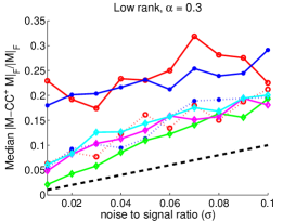
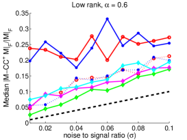
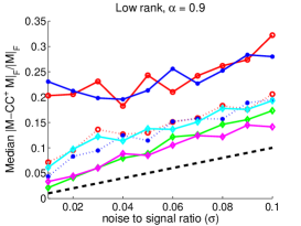
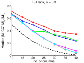
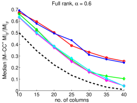
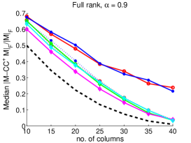
Figure 1: Selection error on Gaussian random matrices. Top row: low-rank plus noise inputs, $s=k=15$; bottom row: full-rank inputs. The black dashed lines denote noise-to-signal ratio $\sigma$ in the first row and $\|\mathbf{M}-\mathbf{M}_{k}\|_{F}$ in the second row. $\alpha$ indicates the observation rate (i.e., the number of observed entries divided by $n_{1}n_{2}$, the total number of matrix entries). All algorithms are run for 8 times on each data set and the median error is reported. We report the median instead of the mean because the performance of norm and leverage score sampling is quite variable.

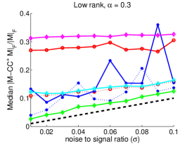
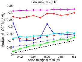
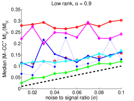
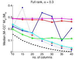
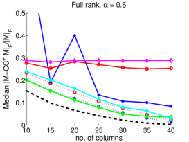
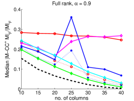
Figure 2: Selection error on matrices with coherent columns. Top row: low-rank plus noise inputs, $s=k=15$; bottom row: full-rank inputs. $\alpha$ indicates the observation rate. The black dashed lines denote noise-to-signal ratio $\sigma$ in the first row and $\|\mathbf{M}-\mathbf{M}_{k}\|_{F}$ in the second row. All algorithms are run for 8 times on each data set and the median error is reported.

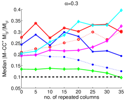
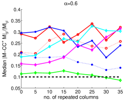
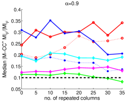
Figure 3: Selection error on matrices with varying number of repeated columns. Both $s$ and $k$ are set to 15 and the noise-to-signal ratio $\sigma$ is set to 0.1. $\alpha$ indicates the observation rate. All algorithms are run for 8 times on each data set and the median error is reported.

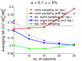
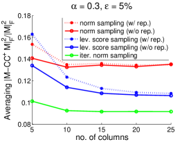
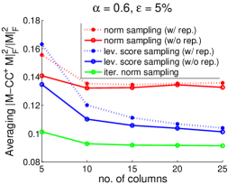
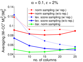
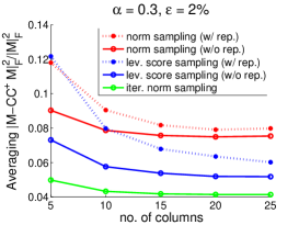
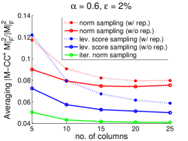
Figure 4: Selection error or sampling based algorithm on Hapmap phase2 data set. $\alpha$ indicates the observation rate. Top row: top-$k$ PCA captures 95% variance within each SNP window; bottom row: top-$k$ PCA captures 98% variance within each SNP window.

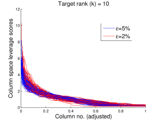
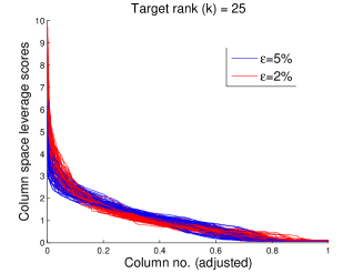
Figure 5: Sorted column space leverage scores for different $\varepsilon$ and $k$ settings. For each setting 50 windows are picked at random and their leverage scores are plotted. Each plotted line is properly scaled along the X axis so that they have the same length even though actual window sizes vary.

(a) The $512\times 512$ 8-bit gray scale Lena test image before compression.

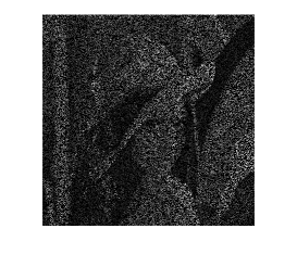
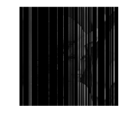
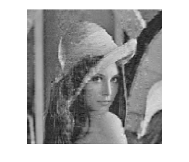
(b) Norm sampling (without replacement). Selection error $\|\mathbf{M}-\mathbf{C}\mathbf{C}^{\dagger}\mathbf{M}\|_{F}/\|\mathbf{M}\|_{F}=0.106$.

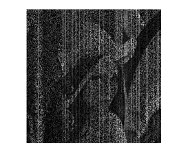
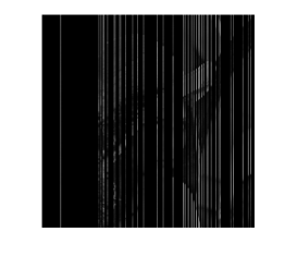
(c) Iterative norm sampling. Selection error $\|\mathbf{M}-\mathbf{C}\mathbf{C}^{\dagger}\mathbf{M}\|_{F}/\|\mathbf{M}\|_{F}=0.088$.

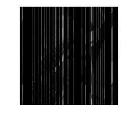
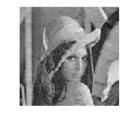
(d) Approx. leverage score sampling (without replacement). $\|\mathbf{M}-\mathbf{C}\mathbf{C}^{\dagger}\mathbf{M}\|_{F}/\|\mathbf{M}\|_{F}=0.103$.

Figure 6: Column-based image compression results on the Lena standard test image. Left: actively sampled image pixels; middle: the selected columns; right: the reconstructed images. Number of selected columns is set to 50 and the pixel subsampling rate $\alpha$ is set to 0.3.

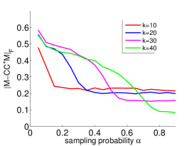
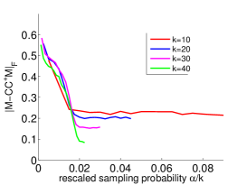
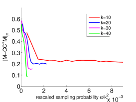
Figure 7: Selection error $\|\mathbf{M}-\mathbf{C}\mathbf{C}^{\dagger}\mathbf{M}\|_{F}$ for the iterative norm sampling algorithm as a function of $\alpha$ (left), $\alpha/k$ (middle) and $\alpha/k^{2}$ (right). Error curves plotted under 4 different rank ($k$) settings.

In this section we report experimental results on both synthetic and real-world data sets for our proposed column subset selection algorithms as well as other competitive methods. All algorithms are implemented in Matlab. To make fair comparisons, all input matrices $\mathbf{M}$ are normalized so that $\|\mathbf{M}\|_{F}^{2}=1$.

6.1 Synthetic data sets

We first test the proposed algorithms on synthetic data sets. The input matrix has dimension $n_{1}=n_{2}=n=50$. To generate the synthetic data, we consider two different settings listed below:

1. Random Gaussian matrices: for random Gaussian matrices each entry $\mathbf{M}_{ij}$ are i.i.d. sampled from a normal distribution $\mathcal{N}(0,1)$. For low rank matrices, we first generate a random Gaussian matrix $\mathbf{B}\in\mathbb{R}^{n\times k}$ where $k$ is the intrinsic rank and then form the data matrix $\mathbf{M}$ as $\mathbf{M}=\mathbf{B}\mathbf{B}^{\top}$. I.i.d. Gaussian noise $\mathbf{R}$ with $\mathbf{R}_{ij}\sim\mathcal{N}(0,\sigma^{2})$ is then appended to the synthesized low-rank matrix. We remark that data matrices generated in this manner have both incoherent column and row space with high probability.

2. Matrices with coherent columns: we took a simple procedure to generate matrices with coherent columns in order to highlight the power of proposed algorithms and baseline methods. After generating a random Gaussian matrix $\mathbf{M}=\mathbf{B}\mathbf{B}^{\top}$, we pick a column $\boldsymbol{x}$ from $\mathbf{M}$ uniformly at random. We then take $\tilde{\boldsymbol{x}}=10\boldsymbol{x}$ and repeat the column for 5 times. As a result, the newly formed data matrix will have 5 identical columns with significantly higher norms compared to the other columns.

In Figure 1 we report the selection error $\|\mathbf{M}-\mathbf{C}\mathbf{C}^{\dagger}\mathbf{M}\|_{F}$ of proposed and baseline algorithms on random Gaussian matrices and in Figure 2 we report the same results on matrices with coherent columns. Results on both low-rank plus noise and high-rank inputs are reported. For low-rank matrices, both the intrinsic rank $k$ and the number of selected columns $s$ are set to 15. Each algorithm is run for 8 times on the same input and the median selection error is reported. For norm sampling and approximate leverage score sampling, we implement two variants: in the sampling with replacement scheme the algorithm samples each column from a sampling distribution (based on either norm or leverage score estimation) with replacement; while in the sampling without replacement scheme a column is never sampled twice. Note that all theoretical results in Section 3 are proved for sampling with replacement algorithms.

From Figure 1 we observe that all algorithms perform similarly, with the exception of two sampling with replacement algorithms and iterative norm sampling when both rank and missing rate are high. For the latter case, we conjecture that the degradation of performance is due to inaccurate norm estimation of column residues; in fact, the iterative norm sampling only provably works when the input matrix has a low-rank plus noise structure (see Theorem 2). On the other hand, when either the target rank or the missing rate is not too high iterative norm sampling works just as good; it is particularly competitive when the true rank of the input matrix is low (see the top row of Figure 1).

When the input matrix has coherent columns, as shown in Figure 2, it becomes easier to observe performance gaps among different algorithms. The block OMP algorithm completely fails in such cases and the selection error for group Lasso also increases considerably. This is due to the fact that both algorithms observe matrix entries by sampling uniformly at random and hence could be poorly informed when the underlying matrix is highly coherent. On the other hand, both leverage score sampling and iterative norm sampling are more robust to column coherence. The coherence among columns also makes the separation between norm sampling and volume sampling clearer in Figure 2. In particular, there is a significant gap between the two sampling with replacement curves and the norm sampling algorithm degrades to its worst-case additive error bound (see Theorem 9). The gap between the sampling without replacement curves is smaller since the coherent column is only repeated for 5 times in the design and so an algorithm can not be “too wrong” if it samples columns without replacement.

To further investigate how the proposed and baseline algorithms adapt to different levels of coherence, we report in Figure 3 the selection error on noisy low-rank matrices with varying number of repeated columns. Matrices with more repeated columns have higher coherence level. We can see that there is a clear separation of two groups of algorithms: the first group includes norm sampling, block OMP and group Lasso, whose error increases as the matrix becomes more coherent. Also, design matrix assumptions (e.g., restricted isometry) are violated for group Lasso. This suggests that these algorithms only have additive error bounds, or adapt poorly to column coherence of the underlying data matrix. On the other hand, the selection error of volume sampling and iterative norm sampling remains stable or slightly decreases. This is consistent with our theoretical results that both volume sampling and iterative norm sampling enjoy relative error bounds.

6.2 Application to tagging Single Nucleotide Polymorphisms (tSNPs) selection

Table 2: Averaging SNP window sizes for different $\varepsilon$ values and number of selected columns per window.

	5 columns	10 columns	15 columns	20 columns	25 columns
$\varepsilon=95\%$	63.4	248.9	516.3	891.0	1405.7
$\varepsilon=98\%$	18.8	62.1	123.4	203.8	309.7

We apply our proposed methods on real-world genetic data sets. We consider the tagging Single Nucleotide Polymorphisms (tSNP) selection task as described in (Ke and Cardon, 2003; Paschou et al., 2007). The task aims at selecting a small set of SNPs in human genes such that the selected SNPs (called tagging SNPs) capture the genetic information within a specific genome region. More specifically, given an $n_{1}\times n_{2}$ matrix with each row corresponding to the genome expression for an individual, we want to select $k$ columns (typically $k\ll n_{2}$) corresponding to $k$ tagging SNPs that best capture the entire SNP matrix across different individuals. Matrix column subset selection methods have been successfully applied to the tSNP selection problem (Paschou et al., 2007).

In this section we demonstrate that our proposed algorithms could achieve the same objective while allowing many missing entries in the raw data matrix. We also compare the selection error of the proposed methods under different missing rate and number of tSNP settings. We did not apply Block OMP and group Lasso because the former cannot handle coherent data matrices and the latter does not scale well. The data set we used is the HapMap Phase 2 data set (international HapMap consortium, 2003). For demonstration purposes, we use gene data for the first chromosome of a joint east Asian population consisting of Han Chinese in Beijing (CHB) and Japanese in Tokyo (JPT). The data matrix consists of 89 rows (individuals) and 311,854 columns (SNPs). Each matrix entry has two letters $b_{1}b_{2}$ describing a specific gene expression for an individual.

We follow the same step as described in (Javed et al., 2011) to preprocess the data. We first convert the raw data matrix into a numerical matrix $\mathbf{M}$ with +1/0/-1 entries as follows: let $B_{1}$ and $B_{2}$ be the bases that appear for the $j$th SNP. Fix an individual $i$ with its gene expression $b_{1}b_{2}$. If $b_{1}b_{2}=B_{1}B_{1}$ then $\mathbf{M}_{ij}$ is set to -1; else if $b_{1}b_{2}=B_{2}B_{2}$ then $\mathbf{M}_{ij}$ is set 1; otherwise $\mathbf{M}_{ij}$ is set to 0. We further split the SNPs into multiple consecutive “windows” so that within each window $w$ the SVD reconstruction error $\|\mathbf{M}^{(w)}-\mathbf{M}^{(w)}_{k}\|_{F}^{2}/\|\mathbf{M}^{(w)}\|_{F}^{2}$ is no larger than $\varepsilon$ with $\varepsilon$ set to 5% and 2%. We refer the readers to Figure 1 in (Javed et al., 2011) for details of the preprocessing steps. Averaging window length (i.e., number of SNPs within each window) are shown in Table 2 for different $k$ and $\varepsilon$ settings. After preprocessing, column subset selection algorithms are performed for each SNP window and the selection error is averaged across all windows, as reported in Figure 4. The number of selected columns per window ($k$) ranges from 5 to 25 and the sampling budget $\alpha$ ranges from 10% to 60%.

In Figure 4 we observe that iterative norm sampling and approximate leverage score sampling outperform norm sampling by a large margin. This is because the truncated data matrix within each window is very close to an exact low-rank matrix and hence relative error algorithms achieve much better performance than additive error ones. In addition, approximate leverage score sampling significantly outperforms norm sampling under both the with replacement and without replacement schemes. This shows that the heterogeneity of human SNPs cannot be captured merely by their norms because the norm is simply the proportion of heterozygous within a population and provides little information about its importance across the entire chromosome. The spikiness of leverage score distribution is empirically verified in Figure 5. Finally, we remark that sampling without replacement is much better than sampling with replacement and should always be preferred in practice. We discuss this aspect in Section 7.5.

6.3 Application to column-based image compression

In this section we show how active sampling can be applied to column-based image compression without observing entire images. Given an image, we first actively subsample a small number of pixels from the original image. We then select a subset of columns based on the observed pixels and reconstruct the entire image by projecting each column to the space spanned by the selected column subsets.

In Figure 6 we depicted the final compressed image as well as intermediate steps (e.g., subsampled pixels and selected columns) on the $512\times 512$ 8-bit gray scale Lena standard test image. We also report the mean and standard deviation of selection error across 10 runs under different settings of target column subset sizes in Table 3.

Table 3 shows that the iterative norm sampling algorithm consistently outperforms norm sampling and so is the leverage score sampling method when the target column subset size is large, which implies small oracle error $\|\mathbf{M}-\mathbf{M}_{k}\|_{F}^{2}$. To get an intuitive sense of why this is the case, we refer the readers to the selected columns for each of the sampling algorithm as shown in Figure 6 (the middle column). It can be seen that the norm sampling algorithm (Figure 6(b)) oversamples columns in relatively easy regions (e.g., the white bar on the left side and the smooth part of the face) because these regions have large pixel values (i.e., they are whiter than the other pixels) and hence have larger column norms. In contrast, the iterative norm sampling algorithm (Figure 6(c)) focuses most sampled columns on the tassel and hair parts which are complicated and cannot be well approximated by other columns. This shows that the iterative norm sampling method has the power to adapt to highly heterogeneous columns and produce better approximations. Finally, we remark that though both leverage score sampling and iterative norm sampling have relative error guarantees, in practice the iterative norm sampling performs much better than leverage score sampling for matrices whose rank is not very high.

7 Discussion

We discuss on several aspects of the proposed algorithms and their analysis.

7.1 Limitation of passive sampling

Table 3: Relative selection error $\|\mathbf{M}-\mathbf{C}\mathbf{C}^{\dagger}\mathbf{M}\|_{F}/\|\mathbf{M}\|_{F}$ on the standard Lena test image ($512\times 512$) for norm sampling (Norm), iterative norm sampling (Iter. norm) and approximate leverage score sampling (Lev. score). Results also compared to a uniform sampling baseline (Uniform) and the truncated SVD lower bound (SVD). The percentage of observed entries $\alpha$ is set to $\alpha=30\%$. Number of columns used for reconstruction varies from 25 to 100.

	Uniform	Norm	Iter. norm	Lev. score	SVD
25 columns	$.151\pm.009$	$.147\pm.004$	$\mathbf{.136\pm.004}$	$.148\pm.007$	$.092$
50 columns	$.104\pm.004$	$.103\pm.003$	$\mathbf{.092\pm.001}$	$.105\pm.003$	$.059$
100 columns	$.064\pm.002$	$.065\pm.001$	$\mathbf{.053\pm.001}$	$.061\pm.002$	$.032$

In most cases the observed entries of a partially observable matrix are sampled according to some sampling schemes. We say a sampling scheme is passive when the sampling distribution (i.e., probability of observing a particular matrix entry) is fixed a priori and does not depend on the data matrix. On the other hand, an active sampling scheme adapts its sampling distribution according to previous observations and requests unknown data points in a feedback driven way. We mainly focus on active sampling methods in this paper (both Algorithm 1 and 2 perform active sampling). However, Algorithm 3 only requires passive sampling because the sampling distribution of rows is the uniform distribution and is fixed a priori.

Passive sampling is known to work poorly for coherent matrices (Krishnamurthy and Singh, 2014; Chen et al., 2013). In this section, we make the following three remarks on the power of passive sampling for column subset selection:

Remark 1

The $\|\mathbf{M}-\mathbf{C}\mathbf{X}\|_{\xi}$ reconstruction error bound for column subset selection is hard for passive sampling. In particular, it can be shown that no passive sampling algorithm achieves relative reconstruction error bound with high probability unless it observes $\Omega(n_{1}n_{2})$ entries of an $n_{1}\times n_{2}$ matrix $\mathbf{M}$. This holds true even if $\mathbf{M}$ is assumed to be exact low rank and has incoherent column space.

This remark can be formalized by noting that when $\mathbf{M}$ is exact low rank then relative reconstruction error implies exact recovery of $\mathbf{M}$, or in other words, matrix completion. Here we cite the hardness result in (Krishnamurthy and Singh, 2014) for completing coherent matrix by passive sampling. Similar results could also be obtained by applying Theorem 6 in (Chen et al., 2013).

Theorem 7 (Theorem 2, (Krishnamurthy and Singh, 2014))

Let $\mathcal{X}$ denote all $n_{1}\times n_{2}$ matrices whose rank is no more than $k$ and column space has incoherence $\mu_{0}$ as defined in Eq. (5). Fix $m<n_{1}n_{2}$ and let $\mathcal{Q}$ denote all passive sampling distributions over $m$ samples of $n_{1}n_{2}$ matrix entries. Let $\mathcal{F}=\{f:\mathbb{R}^{m}\to\mathcal{X}\}$ be the collection of (possibly random) matrix completion algorithms. We then have

$$R_{\mathrm{mc}}^{*}:=\inf_{f\in\mathcal{F}}\inf_{q\in\mathcal{Q}}\sup_{\mathbf{X}\in\mathcal{X}}\Pr_{\Omega\sim q;f}[f(\Omega,\mathbf{X}_{\Omega})\neq\mathbf{X}]\geq\frac{1}{2}-\left\lceil\frac{m}{(1-\frac{k-1}{k\mu_{0}})n_{1}}\right\rceil\frac{1}{2(n-k)},$$ (41)

where $n=\max(n_{1},n_{2})$. As a remark, when $\mu_{0}$ is a constant then $R_{\mathrm{mc}}^{*}=\Omega(1)$ whenever $m=o(n_{1}(n_{2}-k))$.

Remark 2

For the $\|\mathbf{M}-\mathbf{C}\mathbf{C}^{\dagger}\mathbf{M}\|_{\xi}$ selection error (with only column indices $C$ output by an CSS algorithm), it is possible for a passive sampling algorithm to achieve a relative error bound with high probability. In fact, Algorithm 3 and Theorem 3 precisely accomplish this. In addition, when the input matrix is exact low rank, Theorem 3 implies that there exists a passive sampling algorithm that outputs a small subset of columns which span the entire column subspace of a row-coherent matrix with high probability. This result shows column subset selection is easier than matrix completion when only indices of the selected column subset are required. It does not violate Theorem 7, however, because knowing which columns span the column space of an input matrix does not imply we can complete the matrix without further samples.

Remark 3

Although Remark 2 and Theorem 3 shows that it is possible to achieve relative $\|\mathbf{M}-\mathbf{C}\mathbf{C}^{\dagger}\mathbf{M}\|_{F}$ error bound for row coherent matrices via passive sampling, we show in this section that passive sampling is insufficient under a slightly weaker notion of column incoherence. In particular, instead of assuming $\mu(\mathcal{U})\leq\mu_{0}$ on the column space as in Eq. (5), we assume $\mu(\boldsymbol{x}_{i})\leq\mu_{1}$ where $\mu_{1}$ is independent of $k$ for every column $\boldsymbol{x}_{i}$ as in Eq. (7). Note that if $\mathrm{rank}(\mathcal{U})=k$ and $\boldsymbol{x}_{i}\in\mathcal{U}$ then $\mu(\boldsymbol{x}_{i})\leq k\mu(\mathcal{U})$. So for exact low rank matrices the vector-based incoherence assumption in Eq. (7) is weaker than the subspace-based incoherence assumption in Eq. (5). We then have the following theorem, which is proved in Appendix C.

Theorem 8

Let $\mathcal{X}^{\prime}$ denote all $n_{1}\times n_{2}$ matrices whose rank is no more than $k$ and incoherence $\mu_{1}\geq 1+\frac{1}{n_{1}-1}$ as defined in Eq. (7) for each column. Fix $m<n_{1}n_{2}$ and let $\mathcal{Q}$ denote all passive sampling distributions over $m$ samples of $n_{1}n_{2}$ matrix entries. Let $\mathcal{F}^{\prime}=\{f:\mathbb{R}^{m}\to[n_{2}]^{k}\}$ be the collection of (possibly random) column subset selection algorithms. We then have

$$R_{\mathrm{css}}^{*}:=\inf_{f\in\mathcal{F}^{\prime}}\inf_{q\in\mathcal{Q}}\sup_{\mathbf{X}\in\mathcal{X}^{\prime}}\Pr_{\Omega\sim q;f}[\mathbf{X}\neq\mathbf{X}_{C}\mathbf{X}_{C}^{\dagger}\mathbf{X}]\geq\frac{1}{2}-\frac{m}{2n_{1}(n_{2}-k)},$$ (42)

where $C=f(\mathbf{X},\mathbf{X}_{\Omega})$ is the output column subset of $f$. As a remark, the failure probability $R_{\mathrm{css}}^{*}$ satisfies $R_{\mathrm{css}}^{*}=\Omega(1)$ whenever $m=o(n_{1}(n_{2}-k))$.

Theorem 8 combined with Theorem 7 shows a separation of hardness between column subset selection and matrix completion. It also formalizes the intuitive limited power of passive sampling over coherent matrices.

7.2 Time complexity

Table 4: Time complexity of proposed and baseline algorithms. $k$ denotes the intrinsic rank and $s$ denotes the number of selected columns. Dependency on failure probability $\delta$ and other poly-logarithmic dependency is omitted.

Algorithm	Norm	Iter. norm*	Lev. score	Block OMP*	gLasso$\dagger$
Time Complexity	$O(\alpha n^{2})$	$O(\alpha^{2}sn^{3})$	$O(\textrm{svd}(\alpha n,n,k))$	$O(\alpha^{2}sn^{3})$	$O(T(n^{3}+s^{2}n^{2}))$
*Assume $\alpha n>s$ and $\alpha^{2}n>1$.
$\dagger$Using solution path implementation; $T$ is the desired number of $\lambda$ values.

In this section we report the theoretical time complexity of our proposed algorithms as well as the optimization based methods for comparison in Table 4. We assume the input matrix $\mathbf{M}$ is square $n\times n$ and we are using $s$ columns to approximate the top-$k$ component of $\mathbf{M}$. Let $\alpha=m/n^{2}$ be the percentage of observed data. $\mathtt{svd}(a,b,c)$ denotes the time for computing the top-$c$ truncated SVD of an $a\times b$ matrix.

Suppose the observation ratio $\alpha$ is a constant and the $\mathtt{svd}$ operation takes quadratic time. Then the time complexity for all algorithms can be sorted as

$$\textsc{Norm};O(n^{2})<\textsc{Lev. score};O(kn^{2})<\textsc{Iter. norm},\textsc{Block OMP};O(sn^{3})\\ <\textsc{gLasso},O(T(n^{3}+s^{2}n^{2})).$$ (43)

Perhaps not surprisingly, in Section 6.2 and 6.3 on real-world data sets we show the reverse holds for selection error for the first three algorithms in Eq. (43).

7.3 Sample complexity, column subset size and selection error

We remark on the connection of sample complexity (i.e., number of observed matrix entries), size of column subsets and reconstruction error for column subset selection. For column subset selection when the target column subset size is fixed the sample complexity acts more like a threshold: if not enough number of matrix entries are observed then the algorithm fails since the column norms are not accurately estimated, but when a sufficient number of observations are available the reconstruction error does not differ much. Such phase transition was also observed in other matrix completion/approximation tasks as well, for example, in (Krishnamurthy and Singh, 2014). In fact, the guarantee in Eq. (8), for example, is exactly the same as in (Frieze et al., 2004) under the fully observed setting, i.e., $m_{1}=n_{1}$.

The bottom three plots in Figure 2 are an excellent illustration of this phenomenon. When $\alpha=0.3$ the selection error of Algorithm 2 is very high, which means the algorithm does not have enough samples. However, for $\alpha=0.6$ and $\alpha=0.9$ the performance of Algorithm 2 is very similar.

7.4 Sample complexity of the iterative norm sampling algorithm

We try to verify the sample complexity dependence on the intrinsic matrix rank $k$ for the iterative norm sampling algorithm (Algorithm 2). To do this, we run Algorithm 2 under various settings of intrinsic dimension $k$ and the sampling probability $\alpha$ (which is basically proportional to the expected number of per-column samples $m$). We then plot the selection error $\|\mathbf{M}-\mathbf{C}\mathbf{C}^{\dagger}\mathbf{M}\|_{F}$ against $\alpha$, $\alpha/k$ and $\alpha/k^{2}$ in Figure 7.

Theorem 2 states that the dependence of $m$ on $k$ should be $m=\widetilde{O}(k^{2})$ ignoring logarithmic factors. However, in Figure 7 one can observe that when the selection error is plotted against $\alpha/k$ the different curves coincide. This suggests that the actual dependence of $m$ on $k$ should be close to linear instead of quadratic. It is an interesting question whether we can get rid of the use of union bounds over all $n_{2}$-choose-$k$ column subsets in the proof of Theorem 2 in order to get a near linear dependence over $k$. Note that the curves converge to different values for different $k$ settings because selection error decreases when more columns are used to reconstruct the input matrix.

7.5 Sampling with and without replacement

In the experiments we observe that for norm sampling (Algorithm 1) and approximate leverage score sampling (Algorithm 3) the two column sampling schemes, i.e., sampling with and without replacement, makes a big difference in practice (e.g., see Figure 1, 2, and 4). In fact, sampling without replacement always outperforms sampling with replacement because under the latter scheme there is a positive probability of sampling the same column more than once. Though we analyzed both algorithm under the sampling with replacement scheme, in practice sampling without replacement should always be used since it makes no sense to select a column more than once. Finally, we remark that for iterative norm sampling (Algorithm 2) a column will never be picked more than once since the (estimated) projected norm of an already selected column is zero with probability 1.

Acknowledgments

We would like to thank Akshay Krishnamurthy for helpful discussion on the proof of Theorem 2 and James Duyck for a solution path implementation of group Lasso for column subset selection. This work is supported in part by grants NSF-1252412 and AFOSR-FA9550-14-1-0285.

Appendix A Analysis of the active norm sampling algorithm

Proof [Proof of Lemma 1] This lemma is a direct corollary of Theorem 2 from (Frieze et al., 2004). First, let $P_{i}=\hat{c}_{i}/\hat{f}$ be the probability of selecting the $i$-th column of ${\mathbf{M}}$. By assumption, we have $P_{i}\geq\frac{1-\alpha}{1+\alpha}\|\boldsymbol{x}_{i}\|_{2}^{2}/\|\mathbf{M}\|_{F}^{2}$. Applying Theorem 2 from (Frieze et al., 2004) we have that with probability at least $1-\delta$, there exists an orthonormal set of vectors $\boldsymbol{y}^{(1)},\cdots,\boldsymbol{y}^{(k)}\in\mathbb{R}^{n_{1}}$ in $\mathrm{span}(\mathbf{C})$ such that

$$\left\|\mathbf{M}-\left(\sum_{j=1}^{k}{\boldsymbol{y}^{(j)}\boldsymbol{y}^{(j)^{\top}}}\right)\mathbf{M}\right\|_{F}^{2}\leq\|\mathbf{M}-\mathbf{M}_{k}\|_{F}^{2}+\frac{(1+\alpha)k}{(1-\alpha)\delta s}\|\mathbf{M}\|_{F}^{2}.$$ (44)

Finally, to complete the proof, note that every column of $\left(\sum_{j=1}^{k}{\boldsymbol{y}^{(j)}\boldsymbol{y}^{(j)^{\top}}}\right)\mathbf{M}$ can be represented as a linear combination of columns in $\mathbf{C}$; furthermore,

$$\|\mathbf{M}-\mathcal{P}_{C}(\mathbf{M})\|_{F}=\min_{\mathbf{X}\in\mathbb{R}^{k\times n_{2}}}{\|\mathbf{M}-\mathbf{C}\mathbf{X}\|_{F}}\leq\left\|\mathbf{M}-\left(\sum_{j=1}^{k}{\boldsymbol{y}^{(j)}\boldsymbol{y}^{(j)^{\top}}}\right)\mathbf{M}\right\|_{F}.$$ (45)

 

Proof [Proof of Theorem 9] First, set $m_{1}=\Omega(\mu_{0}\log(n_{2}/\delta_{1}))$ we have that with probability $\geq 1-\delta_{1}$ the inequality

$$(1-\alpha)\|\boldsymbol{x}_{i}\|_{2}^{2}\leq\hat{c}_{i}\leq(1+\alpha)\|\boldsymbol{x}_{i}\|_{2}^{2}$$

holds with $\alpha=0.5$ for every column $i$, using Lemma 2. Next, putting $s\geq 6k/\delta_{2}\epsilon^{2}$ and applying Lemma 1 we get

$$\|\mathbf{M}-\mathcal{P}_{C}(\mathbf{M})\|_{F}\leq\|\mathbf{M}-\mathbf{M}_{k}\|_{F}+\epsilon\|\mathbf{M}\|_{F}$$ (46)

with probability at least $1-\delta_{2}$. Finally, note that when $\alpha\leq 1/2$ and $n_{1}\leq n_{2}$ the bound in Lemma 15 is dominated by

$$\|\mathbf{M}-\widehat{\mathbf{M}}\|_{2}\leq\|\mathbf{M}\|_{F}\cdot O\left(\sqrt{\frac{\mu_{0}}{m_{2}}}\log\left(\frac{n_{1}+n_{2}}{\delta}\right)\right).$$ (47)

Consequently, for any $\epsilon^{\prime}>0$ if $m_{2}=\Omega((\epsilon^{\prime})^{-2}\mu_{0}\log^{2}((n_{1}+n_{2})/\delta_{3})$ we have with probability $\geq 1-\delta_{3}$

$$\|\mathbf{M}-\widehat{\mathbf{M}}\|_{2}\leq\epsilon^{\prime}\|\mathbf{M}\|_{F}.$$ (48)

The proof is then completed by taking $\epsilon^{\prime}=\epsilon/\sqrt{s}$:

$$\|\mathbf{M}-\mathbf{C}{\mathbf{X}}\|_{F} = \|\mathbf{M}-\mathcal{P}_{C}(\widehat{\mathbf{M}})\|_{F}$$

$$\leq \|\mathbf{M}-\mathcal{P}_{C}(\mathbf{M})\|_{F}+\|\mathcal{P}_{C}(\mathbf{M}-\widehat{\mathbf{M}})\|_{F}$$

$$\leq \|\mathbf{M}-\mathbf{M}_{k}\|_{F}+\epsilon\|\mathbf{M}\|_{F}+\sqrt{s}\|\mathcal{P}_{C}(\mathbf{M}-\widehat{\mathbf{M}})\|_{2}$$

$$\leq \|\mathbf{M}-\mathbf{M}_{k}\|_{F}+\epsilon\|\mathbf{M}\|_{F}+\sqrt{s}\cdot\epsilon^{\prime}\|\mathbf{M}\|_{F}$$

$$\leq \|\mathbf{M}-\mathbf{M}_{k}\|_{F}+2\epsilon\|\mathbf{M}\|_{F}.$$

 

Appendix B Analysis of the iterative norm sampling algorithm

Proof [Proof of Lemma 17]

We first prove Eq. (16). Observe that $\dim(\mathcal{U}(C))\leq s$. Let $\mathbf{R}_{C}=(\mathbf{R}^{(C(1))},\cdots,\mathbf{R}^{(C(s))})\in\mathbb{R}^{n_{1}\times s}$ denote the selected $s$ columns in the noise matrix $\mathbf{R}$ and let $\mathcal{R}(C)=\mathrm{span}(\mathbf{R}_{C})$ denote the span of selected columns in $\mathbf{R}$. By definition, $\mathcal{U}(C)\subseteq\mathcal{U}\cup\mathcal{R}(C)$, where $\mathcal{U}=\mathrm{span}(\mathbf{A})$ denotes the subspace spanned by columns in the deterministic matrix $\mathbf{A}$. Consequently, we have the following bound on $\|\mathcal{P}_{\mathcal{U}(C)}\boldsymbol{e}_{i}\|$ (assuming each entry in $\mathbf{R}$ follows a zero-mean Gaussian distribution with $\sigma^{2}$ variance):

$$\|\mathcal{P}_{\mathcal{U}(C)}\boldsymbol{e}_{i}\|_{2}^{2} \leq \|\mathcal{P}_{\mathcal{U}}\boldsymbol{e}_{i}\|_{2}^{2}+\|\mathcal{P}_{\mathcal{U}^{\perp}\cap\mathcal{R}(C)}\boldsymbol{e}_{i}\|_{2}^{2}$$

$$\leq \|\mathcal{P}_{\mathcal{U}}\boldsymbol{e}_{i}\|_{2}^{2}+\|\mathcal{P}_{\mathcal{R}(C)}\boldsymbol{e}_{i}\|_{2}^{2}$$

$$\leq \frac{k\mu_{0}}{n_{1}}+\|\mathbf{R}_{C}\|_{2}^{2}\|(\mathbf{R}_{C}^{\top}\mathbf{R}_{C})^{-1}\|_{2}^{2}\|\mathbf{R}_{C}^{\top}\boldsymbol{e}_{i}\|_{2}^{2}$$

$$\leq \frac{k\mu_{0}}{n_{1}}+\frac{(\sqrt{n_{1}}+\sqrt{s}+\epsilon)^{2}\sigma^{2}}{(\sqrt{n_{1}}-\sqrt{s}-\epsilon)^{4}\sigma^{4}}\cdot\sigma^{2}(s+2\sqrt{s\log(2/\delta)}+2\log(2/\delta)).$$

For the last inequality we apply Lemma 65 to bound the largest and smallest singular values of $\mathbf{R}_{C}$ and Lemma 63 to bound $\|\mathbf{R}_{C}^{\top}\boldsymbol{e}_{i}\|_{2}^{2}$, because $\mathbf{R}_{C}^{\top}\boldsymbol{e}_{i}$ follow i.i.d. Gaussian distributions with covariance $\sigma^{2}\mathbf{I}_{s\times s}$. If $\epsilon$ is set as $\epsilon=\sqrt{2\log(4/\delta)}$ then the last inequality holds with probability at least $1-\delta$. Furthermore, when $s\leq n_{1}/2$ and $\delta$ is not exponentially small (e.g., $\sqrt{2\log(4/\delta)}\leq\frac{\sqrt{n_{1}}}{4}$), the fraction $\frac{(\sqrt{n_{1}}+\sqrt{s}+\epsilon)^{2}}{(\sqrt{n_{1}}-\sqrt{s}-\epsilon)^{4}}$ is approximately $O(1/n_{1})$. As a result, with probability $1-n_{1}\delta$ the following holds:

$$\mu(\mathcal{U}(C))=\frac{n_{1}}{s}\max_{1\leq i\leq n_{1}}{\|\mathcal{P}_{\mathcal{U}(C)}\boldsymbol{e}_{i}\|_{2}^{2}}\\ \leq\frac{n_{1}}{s}\left(\frac{k\mu_{0}}{n_{1}}+O\left(\frac{s+\sqrt{s\log(1/\delta)}+\log(1/\delta)}{n_{1}}\right)\right)=O\left(\frac{k\mu_{0}+s+\sqrt{s\log(1/\delta)}+\log(1/\delta)}{s}\right).$$ (49)

Finally, putting $\delta^{\prime}=n_{1}/\delta$ we prove Eq. (16).

Next we try to prove Eq. (17). Let $\boldsymbol{x}$ be the $i$-th column of $\mathbf{M}$ and write $\boldsymbol{x}=\boldsymbol{a}+\boldsymbol{r}$, where $\boldsymbol{a}=\mathcal{P}_{\mathcal{U}}(\boldsymbol{x})$ and $\boldsymbol{r}=\mathcal{P}_{\mathcal{U}^{\perp}}(\boldsymbol{x})$. Since the deterministic component of $\boldsymbol{x}$ lives in $\mathcal{U}$ and the random component of $\boldsymbol{x}$ is a vector with each entry sampled from i.i.d. zero-mean Gaussian distributions, we know that $\boldsymbol{r}$ is also a zero-mean random Gaussian vector with i.i.d. sampled entries. Note that $\mathcal{U}(C)$ does not depend on the randomness over $\{\mathbf{M}^{(i)}:i\notin C\}$. Therefore, in the following analysis we will assume $\mathcal{U}(C)$ to be a fixed subspace $\widetilde{\mathcal{U}}$ with dimension at most $s$.

The projected vector $\boldsymbol{x}^{\prime}=\mathcal{P}_{\widetilde{\mathcal{U}}^{\perp}}\boldsymbol{x}$ can be written as $\tilde{\boldsymbol{x}}=\tilde{\boldsymbol{a}}+\tilde{\boldsymbol{r}}$, where $\tilde{\boldsymbol{a}}=\mathcal{P}_{\widetilde{\mathcal{U}}^{\perp}}\boldsymbol{a}$ and $\tilde{\boldsymbol{r}}=\mathcal{P}_{\widetilde{\mathcal{U}}^{\perp}}\boldsymbol{r}$. By definition, $\tilde{\boldsymbol{a}}$ lives in the subspace $\mathcal{U}\cap\widetilde{\mathcal{U}}^{\perp}$. So it satisfies the incoherence assumption

$$\mu(\tilde{\boldsymbol{a}})=\frac{n_{1}\|\tilde{\boldsymbol{a}}\|_{\infty}^{2}}{\|\tilde{\boldsymbol{a}}\|_{2}^{2}}\leq k\mu(\mathcal{U})\leq k\mu_{0}.$$ (50)

On the other hand, because $\tilde{\boldsymbol{r}}$ is an orthogonal projection of some random Gaussian variable, $\tilde{\boldsymbol{r}}$ is still a Gaussian random vector, which lives in $\mathcal{U}^{\perp}\cap\widetilde{\mathcal{U}}^{\perp}$ with rank at least $n_{1}-k-s$. Subsequently, we have

$$\mu(\tilde{\boldsymbol{x}}) = n_{1}\frac{\|\tilde{\boldsymbol{x}}\|_{\infty}^{2}}{\|\tilde{\boldsymbol{x}}\|_{2}^{2}}\leq 3n_{1}\frac{\|\tilde{\boldsymbol{a}}\|_{\infty}^{2}+\|\tilde{\boldsymbol{r}}\|_{\infty}^{2}}{\|\tilde{\boldsymbol{a}}\|_{2}^{2}+\|\tilde{\boldsymbol{r}}\|_{2}^{2}}$$

$$\leq 3n_{1}\frac{\|\tilde{\boldsymbol{a}}\|_{\infty}^{2}}{\|\tilde{\boldsymbol{a}}\|_{2}^{2}}+3n_{1}\frac{\|\tilde{\boldsymbol{r}}\|_{\infty}^{2}}{\|\tilde{\boldsymbol{r}}\|_{2}^{2}}$$

$$\leq 3k\mu_{0}+\frac{6\sigma^{2}n_{1}\log(2n_{1}n_{2}/\delta)}{\sigma^{2}(n_{1}-k-s)-2\sigma^{2}\sqrt{(n_{1}-k-s)\log(n_{2}/\delta)}}.$$

For the second inequality we use the fact that $\frac{\sum_{i}{a_{i}}}{\sum_{i}{b_{i}}}\leq\sum_{i}{\frac{a_{i}}{b_{i}}}$ whenever $a_{i},b_{i}\geq 0$. For the last inequality we use Lemma 64 on the enumerator and Lemma 63 on the denominator. Finally, note that when $\max(s,k)\leq n_{1}/4$ and $\log(n_{2}/\delta)\leq n_{1}/64$ the denominator can be lower bounded by $\sigma^{2}n_{1}/4$; subsequently, we can bound $\mu(\tilde{\boldsymbol{x}})$ as

$$\mu(\tilde{\boldsymbol{x}})\leq 3k\mu_{0}+\frac{24\sigma^{2}n_{1}\log(2n_{1}n_{2}/\delta)}{\sigma^{2}n_{1}}\leq 3k\mu_{0}+24\log(2n_{1}n_{2}/\delta).$$ (51)

Taking a union bound over all $n_{2}-s$ columns yields the result.

 

To prove the norm estimation consistency result in Lemma 5 we first cite a seminal theorem from (Krishnamurthy and Singh, 2014) which provides a tight error bound on a subsampled projected vector in terms of the norm of the true projected vector.

Theorem 9

Let $\mathcal{U}$ be a $k$-dimensional subspace of $\mathbb{R}^{n}$ and $\boldsymbol{y}=\boldsymbol{x}+\boldsymbol{v}$, where $\boldsymbol{x}\in\mathcal{U}$ and $\boldsymbol{v}\in\mathcal{U}^{\perp}$. Fix $\delta^{\prime}>0$, $m\geq\max\{\frac{8}{3}k\mu(\mathcal{U})\log\left(\frac{2k}{\delta^{\prime}}\right),4\mu(\boldsymbol{v})\log(1/\delta^{\prime})\}$ and let $\Omega$ be an index set with entries sampled uniformly with replacement with probability $m/n$. Then with probability at least $1-4\delta^{\prime}$:

$$\frac{m(1-\alpha)-k\mu(\mathcal{U})\frac{\beta}{1-\gamma}}{n}\|\boldsymbol{v}\|_{2}^{2}\leq\|\boldsymbol{y}_{\Omega}-\mathcal{P}_{U_{\Omega}}\boldsymbol{y}_{\Omega}\|_{2}^{2}\leq(1+\alpha)\frac{m}{n}\|\boldsymbol{v}\|_{2}^{2},$$ (52)

where $\alpha=\sqrt{2\frac{\mu(\boldsymbol{v})}{m}\log(1/\delta^{\prime})}+2\frac{\mu(\boldsymbol{v})}{3m}\log(1/\delta^{\prime})$, $\beta=(1+2\sqrt{\log(1/\delta^{\prime})})^{2}$ and $\gamma=\sqrt{\frac{8k\mu(\mathcal{U})}{3m}\log(2k/\delta^{\prime})}$.

We are now ready to prove Lemma 5.

Proof [Proof of Lemma 5] By Algorithm 2, we know that $\dim(\mathcal{S}_{t})=t$ with probability 1. Let $\boldsymbol{y}=\mathbf{M}^{(i)}$ denote the $i$-th column of $\mathbf{M}$ and let $\boldsymbol{v}=\mathcal{P}_{\mathcal{S}_{t}}\boldsymbol{y}$ be the projected vector. We can apply Theorem 9 to bound the estimation error between $\|\boldsymbol{v}\|$ and $\|\boldsymbol{y}_{\Omega}-\mathcal{P}_{\mathcal{S}_{t}(\Omega)}\boldsymbol{y}_{\Omega}\|$.

First, when $m$ is set as in Eq. (20) it is clear that the conditions $m\geq\frac{8}{3}t\mu(\mathcal{U})\log\left(\frac{2t}{\delta^{\prime}}\right)=\Omega(k\mu_{0}\log(n/\delta)\log(k/\delta^{\prime}))$ and $m\geq 4\mu(\boldsymbol{v})\log(1/\delta^{\prime})=\Omega(k\mu_{0}\log(n/\delta)\log(1/\delta^{\prime}))$ are satisfied. We next turn to the analysis of $\alpha$, $\beta$ and $\gamma$. More specifically, we want $\alpha=O(1)$, $\gamma=O(1)$ and $\frac{t\mu(\mathcal{U})}{m}\beta=O(1)$.

For $\alpha$, $\alpha=O(1)$ implies $m=\Omega(\mu(\boldsymbol{v})\log(1/\delta^{\prime}))=\Omega(k\mu_{0}\log(n/\delta)\log(1/\delta^{\prime}))$. Therefore, by carefully selecting constants in $\Omega(\cdot)$ we can make $\alpha\leq 1/4$.

For $\gamma$, $\gamma=O(1)$ implies $m=\Omega(t\mu(\mathcal{U})\log(t/\delta^{\prime}))=\Omega(k\mu_{0}\log(n/\delta)\log(k/\delta^{\prime}))$. By carefully selecting constants in $\Omega(\cdot)$ we can make $\gamma\leq 0.2$.

For $\beta$, $\frac{t\mu(\mathcal{U})}{m}\beta=O(1)$ implies $m=O(t\mu(\mathcal{U})\beta)=O(k\mu_{0}\log(n/\delta)\log(1/\delta^{\prime}))$. By carefully selecting constants we can have $\beta\leq 0.2$. Finally, combining bounds on $\alpha$, $\beta$ and $\gamma$ we prove the desired result.  

Before proving Lemma 27, we first cite a lemma from (Deshpande et al., 2006) that connects the volume of a simplex to the permutation sum of singular values.

Lemma 9 ((Deshpande et al., 2006))

Fix $\mathbf{A}\in\mathbb{R}^{m\times n}$ with $m\leq n$. Suppose $\sigma_{1},\cdots,\sigma_{m}$ are singular values of $\mathbf{A}$. Then

$$\sum_{S\subseteq[n],|S|=k}{\mathrm{vol}(\Delta(S))^{2}}=\frac{1}{(k!)^{2}}\sum_{1\leq i_{1}<i_{2}<\cdots<i_{k}\leq m}{\sigma_{i_{1}}^{2}\sigma_{i_{2}}^{2}\cdots\sigma_{i_{k}}^{2}}.$$ (53)

Now we are ready to prove Lemma 27.

Proof [Proof of Lemma 27] Let $\mathbf{M}_{k}$ denote the best rank-$k$ approximation of $\mathbf{M}$ and assume the singular values of $\mathbf{M}$ are $\{\sigma_{i}\}_{i=1}^{n_{1}}$. Let $C=\{i_{1},\cdots,i_{k}\}$ be the selected columns. Let $\tau\in\Pi_{k}$, where $\Pi_{k}$ denotes all permutations with $k$ elements. By $\mathcal{H}_{\tau,t}$ we denote the linear subspace spanned by $\{\mathbf{M}^{(\tau(i_{1}))},\cdots,\mathbf{M}^{(\tau(i_{t}))}\}$ and let $d(\mathbf{M}^{(i)},\mathcal{H}_{\tau,t})$ denote the distance between column $\mathbf{M}^{(i)}$ and subspace $\mathcal{H}_{\tau,t}$. We then have

$$\hat{p}_{C} \leq \sum_{\tau\in\Pi_{k}}{\left(\frac{5}{2}\right)^{k}\frac{\|\mathbf{M}^{(\tau(i_{1}))}\|_{2}^{2}}{\|\mathbf{M}\|_{F}^{2}}\frac{d(\mathbf{M}^{(\tau(i_{2}))},\mathcal{H}_{\tau,1})^{2}}{\sum_{i=1}^{n_{2}}{d(\mathbf{M}^{(i)},\mathcal{H}_{\tau,1})^{2}}}\cdots\frac{d(\mathbf{M}^{(\tau(i_{k}))},\mathcal{H}_{\tau,k-1})^{2}}{\sum_{i=1}^{n_{2}}{d(\mathbf{M}^{(i)},\mathcal{H}_{\tau,k-1})^{2}}}}$$

$$\leq 2.5^{k}\cdot\frac{\sum_{\tau\in\Pi_{k}}{\|\mathbf{M}^{(\tau(i_{1}))}\|^{2}d(\mathbf{M}^{(\tau(i_{2}))},\mathcal{H}_{\tau,1})^{2}\cdots d(\mathbf{M}^{(\tau(i_{k}))},\mathcal{H}_{\tau,k-1})^{2}}}{\|\mathbf{M}\|_{F}^{2}\|\mathbf{M}-\mathbf{M}_{1}\|_{F}^{2}\cdots\|\mathbf{M}-\mathbf{M}_{k-1}\|_{F}^{2}}$$

$$= 2.5^{k}\cdot\frac{\sum_{\tau\in\Pi_{k}}{(k!)^{2}\mathrm{vol}(\Delta(C))^{2}}}{\|\mathbf{M}\|_{F}^{2}\|\mathbf{M}-\mathbf{M}_{1}\|_{F}^{2}\cdots\|\mathbf{M}-\mathbf{M}_{k-1}\|_{F}^{2}}$$

$$= 2.5^{k}\cdot\frac{(k!)^{3}\mathrm{vol}(\Delta(C))^{2}}{\sum_{i=1}^{n_{1}}{\sigma_{i}^{2}}\sum_{i=2}^{n_{1}}{\sigma_{i}^{2}}\cdots\sum_{i=k}^{n_{1}}{\sigma_{i}^{2}}}$$

$$\leq 2.5^{k}\cdot\frac{(k!)^{3}\mathrm{vol}(\Delta(C))^{2}}{\sum_{1\leq i_{1}<i_{2}<\cdots<i_{k}\leq n_{1}}{\sigma_{i_{1}}^{2}\sigma_{i_{2}}^{2}\cdots\sigma_{i_{k}}^{2}}}$$

$$= 2.5^{k}\cdot\frac{k!\mathrm{vol}(\Delta(C))^{2}}{\sum_{T:|T|=k}{\mathrm{vol}(\Delta(T))^{2}}}=2.5^{k}k!p_{C}.$$

For the first inequality we apply Eq. (23) and for the second to last inequality we apply Lemma 53.  

Lemma 31 can be proved by applying Theorem 5 for $T$ rounds, given the norm estimation accuracy bound in Proposition 1.

Proof [Proof of Lemma 31] First note that

$$\|\mathbf{M}-\mathcal{P}_{\mathcal{U}\cup\mathcal{S}_{1}\cup\cdots\cup\mathcal{S}_{T}}(\mathbf{M})\|_{F}^{2}\leq\|\mathbf{M}-\mathcal{P}_{\mathcal{U}\cup\mathcal{S}_{1}\cup\cdots\cup\mathcal{S}_{T},k}(\mathbf{M})\|_{F}^{2}.$$

Applying Theorem 5 with $\frac{1+\alpha}{1-\alpha}=\frac{5}{2}$, we have

$$\mathbb{E}\left[\|\mathbf{M}-\mathcal{P}_{\mathcal{U}\cup\mathcal{S}_{1}\cup\cdots\cup\mathcal{S}_{T}}(\mathbf{M})\|_{F}^{2}\right]$$

$$\leq \|\mathbf{M}-\mathbf{M}_{k}\|_{F}^{2}+\frac{5k}{2s_{T}}\mathbb{E}\left[\|\mathbf{M}-\mathcal{P}_{\mathcal{U}\cup\mathcal{S}_{1}\cup\cdots\mathcal{S}_{T-1}}(\mathbf{M})\|_{F}\right]^{2}$$

$$\leq \|\mathbf{M}-\mathbf{M}_{k}\|_{F}^{2}+\frac{5k}{2s_{T}}\left(\|\mathbf{M}-\mathbf{M}_{k}\|_{F}^{2}+\frac{5k}{2s_{T-1}}\mathbb{E}\left[\|\mathbf{M}-\mathcal{P}_{\mathcal{U}\cup\mathcal{S}_{1}\cup\cdots\mathcal{S}_{T-2}}(\mathbf{M})\|_{F}^{2}\right]\right)$$

$$\leq \cdots$$

$$\leq \left(1+\frac{5}{2}\frac{k}{s_{T}}+\left(\frac{5}{2}\right)^{2}\frac{k^{2}}{s_{T}s_{T-1}}+\cdots+\left(\frac{5}{2}\right)^{T-1}\frac{k^{T-1}}{s_{T-1}\cdots s_{1}}\right)\|\mathbf{M}-\mathbf{M}_{k}\|_{F}^{2}$$

$$+\left(\frac{5}{2}\right)^{T}\frac{k^{T}}{s_{T}s_{T-1}\cdots s_{1}}\|\mathbf{M}-\mathcal{P}_{\mathcal{U}}(\mathbf{M})\|_{F}^{2}$$

$$\leq \left(1+\frac{\epsilon}{4\delta}+\frac{\epsilon}{20\delta}+\cdots\right)\|\mathbf{M}-\mathbf{M}_{k}\|_{F}^{2}+\frac{\epsilon/2}{2^{T}\delta}\|\mathbf{E}\|_{F}^{2}$$

$$\leq \left(1+\frac{\epsilon}{2\delta}\right)\|\mathbf{M}-\mathbf{M}_{k}\|_{F}^{2}+\frac{\epsilon/2}{2^{T}\delta}\|\mathbf{E}\|_{F}^{2}.$$

Finally applying Markov’s inequality we complete the proof.  

To prove the reconstruction error bound in Lemma 34 we need the following two technical lemmas, cited from (Krishnamurthy and Singh, 2013; Balzano et al., 2010b).

Lemma 10 ((Krishnamurthy and Singh, 2013))

Suppose $\mathcal{U}\subseteq\mathbb{R}^{n}$ has dimension $k$ and $\mathbf{U}\in\mathbb{R}^{n\times k}$ is the orthogonal matrix associated with $\mathcal{U}$. Let $\Omega\subseteq[n]$ be a subset of indices each sampled from i.i.d. Bernoulli distributions with probability $m/n_{1}$. Then for some vector $\boldsymbol{y}\in\mathbb{R}^{n}$, with probability at least $1-\delta$:

$$\|\mathbf{U}_{\Omega}^{\top}\boldsymbol{y}_{\Omega}\|_{2}^{2}\leq\beta\frac{m}{n_{1}}\frac{k\mu(\mathcal{U})}{n_{1}}\|\boldsymbol{y}\|_{2}^{2},$$ (54)

where $\beta$ is defined in Theorem 9.

Lemma 11 ((Balzano et al., 2010b))

With the same notation in Lemma 10 and Theorem 9. With probability $\geq 1-\delta$ one has

$$\|(\mathbf{U}_{\Omega}^{\top}\mathbf{U}_{\Omega})^{-1}\|\leq\frac{n_{1}}{(1-\gamma)m},$$ (55)

provided that $\gamma<1$.

Now we can prove Lemma 34.

Proof [Proof of Lemma 34] Let $\mathcal{U}=\mathcal{U}(S)$ and $\mathbf{U}\in\mathbb{R}^{n_{1}\times s}$ be the orthogonal matrix associated with $\mathcal{U}$. Fix a column $i$ and let $\boldsymbol{x}=\mathbf{M}^{(i)}=\boldsymbol{a}+\boldsymbol{r}$, where $\boldsymbol{a}\in\mathcal{U}$ and $\boldsymbol{r}\in\mathcal{U}^{\perp}$. What we want is to bound $\|\boldsymbol{x}-\mathbf{U}(\mathbf{U}_{\Omega}^{\top}\mathbf{U}_{\Omega})^{-1}\mathbf{U}_{\Omega}^{\top}\boldsymbol{x}_{\Omega}\|_{2}^{2}$ in terms of $\|\boldsymbol{r}\|_{2}^{2}$.

Write $\boldsymbol{a}=\mathbf{U}\boldsymbol{\tilde{a}}$. By Lemma 11, if $m$ satisfies the condition given in the Lemma then with probability over $1-\delta-\delta^{\prime\prime}$ we know $(\mathbf{U}_{\Omega}^{\top}\mathbf{U}_{\Omega})$ is invertible and furthermore, $\|(\mathbf{U}_{\Omega}^{\top}\mathbf{U}_{\Omega})^{-1}\|_{2}\leq 2n_{1}/m$. Consequently,

$$\mathbf{U}(\mathbf{U}_{\Omega}^{\top}\mathbf{U}_{\Omega})^{-1}\mathbf{U}_{\Omega}^{\top}\boldsymbol{a}_{\Omega}=\mathbf{U}(\mathbf{U}_{\Omega}^{\top}\mathbf{U}_{\Omega})^{-1}\mathbf{U}_{\Omega}^{\top}\mathbf{U}_{\Omega}\tilde{\boldsymbol{a}}=\mathbf{U}\tilde{\boldsymbol{a}}=\boldsymbol{a}.$$ (56)

That is, the subsampled projector preserves components of $\boldsymbol{x}$ in subspace $\mathcal{U}$.

Now let’s consider the noise term $\boldsymbol{r}$. By Corollary 19 with probability $\geq 1-\delta$ we can bound the incoherence level of $\boldsymbol{y}$ as $\mu(\boldsymbol{y})=O(s\mu_{0}\log(n/\delta))$. The incoherence of subspace $\mathcal{U}$ can also be bounded as $\mu(\mathcal{U})=O(\mu_{0}\log(n/\delta))$. Subsequently, given $m=\Omega(\epsilon^{-1}s\mu_{0}\log(n/\delta)\log(n/\delta^{\prime\prime}))$ we have (with probability $\geq 1-\delta-2\delta^{\prime\prime}$)

$$\|\boldsymbol{x}-\mathbf{U}(\mathbf{U}_{\Omega}^{\top}\mathbf{U}_{\Omega})^{-1}\mathbf{U}_{\Omega}^{\top}(\boldsymbol{a}+\boldsymbol{r})|_{2}^{2}$$

$$= \|\boldsymbol{a}+\boldsymbol{r}-\mathbf{U}(\mathbf{U}_{\Omega}^{\top}\mathbf{U}_{\Omega})^{-1}\mathbf{U}_{\Omega}^{\top}(\boldsymbol{a}+\boldsymbol{r})\|_{2}^{2}$$

$$= \|\boldsymbol{r}-\mathbf{U}(\mathbf{U}_{\Omega}^{\top}\mathbf{U}_{\Omega})^{-1}\mathbf{U}_{\Omega}^{\top}\boldsymbol{r}\|_{2}^{2}$$

$$\leq \|\boldsymbol{r}\|_{2}^{2}+\|(\mathbf{U}_{\Omega}^{\top}\mathbf{U}_{\Omega})^{-1}\|_{2}^{2}\|\mathbf{U}_{\Omega}^{\top}\boldsymbol{r}\|_{2}^{2}$$

$$\leq (1+O(\epsilon))\|\boldsymbol{r}\|_{2}^{2}.$$

For the second to last inequality we use the fact that $\boldsymbol{r}\in\mathcal{U}^{\perp}$. By carefully selecting constants in Eq. (22) we can make

$$\|\boldsymbol{x}-\mathbf{U}(\mathbf{U}_{\Omega}^{\top}\mathbf{U}_{\Omega})^{-1}\mathbf{U}_{\Omega}^{\top}\boldsymbol{x}\|_{2}^{2}\leq(1+\epsilon)\|\mathcal{P}_{\mathcal{U}^{\perp}}\boldsymbol{x}\|_{2}^{2}.$$ (57)

Summing over all $n_{2}$ columns yields the desired result.  

Appendix C Proof of lower bound for passive sampling

Proof [Proof of Theorem 8] Let $\widetilde{\mathcal{X}}=\{\mathbf{X}_{1},\cdots,\mathbf{X}_{T}\}\subseteq\mathcal{X}^{\prime}$ be a finite subset of $\mathcal{X}^{\prime}$ which we specify later. Let $\pi$ be any prior distribution over $\widetilde{\mathcal{X}}$. We then have the following chain of inequalities:

$$R_{\mathrm{css}}^{*} = \inf_{f\in\mathcal{F}^{\prime}}\inf_{q\in\mathcal{Q}}\sup_{\mathbf{X}\in\mathcal{X}^{\prime}}\Pr_{\Omega\sim q;f}[\mathbf{X}\neq\mathbf{X}_{C}\mathbf{X}_{C}^{\dagger}\mathbf{X}]$$ (58)

$$\geq \inf_{f\in\mathcal{F}^{\prime}}\inf_{q\in\mathcal{Q}}\Pr_{\Omega\sim q;\mathbf{X}\sim\pi;f}[\mathbf{X}\neq\mathbf{X}_{C}\mathbf{X}_{C}^{\dagger}\mathbf{X}]$$

$$\geq \inf_{f\in\mathcal{F}^{\prime}}\min_{|\Omega|=m}\Pr_{\mathbf{X}\sim\pi;f}[\mathbf{X}\neq\mathbf{X}_{C}\mathbf{X}_{C}^{\dagger}\mathbf{X}].$$ (59)

Here Eq. (58) uses the fact that the maximum dominates any expectation over the same set and for Eq. (59) we apply Yao’s principle, which asserts that the worst-case performance of a randomized algorithm is better (i.e., lower bounded) by the averaging performance of a deterministic algorithm. Hence, when the input matrix $\mathbf{X}$ is randomized by a prior $\pi$ it suffices to consider only deterministic sampling schemes, which corresponds to a subset of matrix entries $\Omega$ fixed a priori, with size $|\Omega|=m$.

We next construct the subset $\widetilde{\mathcal{X}}$ and let $\pi$ be the uniform distribution over $\widetilde{\mathcal{X}}$. Let $\boldsymbol{x}_{1},\cdots,\boldsymbol{x}_{k-2}\in\mathbb{R}^{n_{1}}$ be an arbitrary set of linear independent column vectors with $[\boldsymbol{x}_{i}]_{1}=0$ for all $i=1,2,\cdots,k=2$ and $\mu(\boldsymbol{x}_{1}),\cdots,\mu(\boldsymbol{x}_{k-2})=1+\frac{1}{n_{1}-1}$. This can be done by setting all nonzero entries in $\boldsymbol{x}_{1},\cdots,\boldsymbol{x}_{k-2}$ to $\pm 1$. In addition, we define $\boldsymbol{y}:=(1,1,\cdots,1)$ and $\boldsymbol{e}_{j}=(0,\cdots,0,1,0,\cdots,0)$ with the only nonzero entry at the $j$th position. Next, define $\widetilde{\mathbf{X}}=\{\mathbf{X}^{i,j}\}_{i=k-1,j=1}^{n_{2},n_{1}}$ with

$$\mathbf{X}^{i,j}_{(\ell)}=\left\{\begin{array}[]{ll}\boldsymbol{x}_{\ell}&\text{if }\ell\leq k-2,\\ \boldsymbol{y}-2\boldsymbol{e}_{j}&\text{if }\ell=i,\\ \boldsymbol{y}&\text{otherwise.}\end{array}\right.$$ (60)

It follows by definition that $\mathrm{rank}(\mathbf{X}^{i,j})=k$ and $\mu(\mathbf{X}^{i,j}_{(\ell)})\leq\mu_{1}=1+\frac{1}{n_{1}-1}$ for all $i,j$ and $\ell$. Furthermore, for fixed $i$ and $j$ one necessary condition for $\mathbf{X}=\mathbf{X}_{C}\mathbf{X}_{C}^{\dagger}\mathbf{X}$ is $\{1,2,\cdots,k-2,i\}\subseteq C$. Therefore, if for distinct $i_{1},i_{2},i_{3},i_{4}$ and some $j_{1},j_{2},j_{3},j_{4}$ one has $\mathbf{X}^{i_{1},j_{1}}_{\Omega}=\cdots=\mathbf{X}^{i_{4},j_{4}}_{\Omega}$ then the best a column subset selection algorithm $f$ could do is random guessing and hence $\Pr[\mathbf{X}\neq\mathbf{X}_{C}\mathbf{X}_{C}^{\dagger}\mathbf{X}]\geq 1/2$. Consequently, for fixed $\Omega$ one has

$$\inf_{f\in\mathcal{F}^{\prime}}\Pr_{\mathbf{X}\sim\pi;f}[\mathbf{X}\neq\mathbf{X}_{C}\mathbf{X}_{C}^{\dagger}\mathbf{X}]\geq\frac{1}{2}-\frac{1}{2}\bigg{|}\left\{\mathbf{X}^{i,j}:\mathbf{X}^{i^{\prime},j^{\prime}}_{\Omega}\neq\mathbf{X}^{i,j},\forall i^{\prime}\neq i,j^{\prime}\in[n_{1}]\right\}\bigg{|}.$$ (61)

The final step is to bound the size of the set $E=\{\mathbf{X}^{i,j}:\mathbf{X}^{i^{\prime},j^{\prime}}_{\Omega}\neq\mathbf{X}^{i,j},\forall i^{\prime}\neq i,j^{\prime}\in[n_{1}]\}$. Note that if $\mathbf{X}_{\Omega}$ is $+1$ on all entries $(i,j)$ with $i>k-2$ then $\mathbf{X}\notin E$ because for every $\mathbf{X}^{\prime}\in\widetilde{\mathcal{X}}$, $\mathbf{X}^{\prime}_{\Omega}=\mathbf{X}_{\Omega}$. Consequently,

$$\big{|}E\big{|}\leq\frac{|\Omega|}{n_{1}(n_{2}-k+2)}\leq\frac{m}{n_{1}(n_{2}-k)}.$$ (62)

Plugging Eq. (62) into Eq. (61) we complete the proof of Theorem 8.

 

Appendix D Some concentration inequalities

Lemma 12 ((Laurent and Massart, 2000))

Let $X\sim\chi_{d}^{2}$. Then with probability $\geq 1-2\delta$ the following holds:

$$-2\sqrt{d\log(1/\delta)}\leq X-d\leq 2\sqrt{d\log(1/\delta)}+2\log(1/\delta).$$ (63)

Lemma 13

Let $X_{1},\cdots,X_{n}\sim\mathcal{N}(0,\sigma^{2})$. Then with probability $\geq 1-\delta$ the following holds:

$$\max_{i}{|X_{i}|}\leq\sigma\sqrt{2\log(2n/\delta)}.$$ (64)

Lemma 14 ((Vershynin, 2010))

Let $\mathbf{X}$ be an $n\times t$ random matrix with i.i.d. standard Gaussian random entries. If $t<n$ then for every $\epsilon\geq 0$ with probability $\geq 1-2\exp(-\epsilon^{2}/2)$ the following holds:

$$\sqrt{n}-\sqrt{t}-\epsilon\leq\sigma_{\min}(\mathbf{X})\leq\sigma_{\max}(\mathbf{X})\leq\sqrt{n}+\sqrt{t}+\epsilon.$$ (65)

Lemma 15 (Noncommutative Bernstein Inequality, (Gross et al., 2010; Recht, 2011))

Let $\mathbf{X}_{1},\cdots,\mathbf{X}_{m}$ be independent zero-mean square $n\times n$ random matrices. Suppose $\rho_{k}^{2}=\max(\|\mathbb{E}[\mathbf{X}_{k}\mathbf{X}_{k}^{\top}]\|_{2},\|\mathbb{E}[\mathbf{X}_{k}^{\top}\mathbf{X}_{k}]\|_{2})$ and $\|\mathbf{X}_{k}\|_{2}\leq M$ with probability 1 for all $k$. Then for any $t>0$,

$$\Pr\left[\left\|\sum_{k=1}^{m}{\mathbf{X}_{k}}\right\|_{2}>t\right]\leq 2n\exp\left(-\frac{t^{2}/2}{\sum_{k=1}^{m}{\rho_{k}^{2}}+Mt/3}\right).$$ (66)

References

• Achlioptas and McSherry (2007) Dimitris Achlioptas and Frank McSherry. Fast computation of low-rank matrix approximations. Journal of the ACM, 2007.
• Achlioptas et al. (2013) Dimitris Achlioptas, Zohar Karnin, and Edo Liberty. Near-optimal entrywise sampling for data matrices. In Proceedings of Advances in Neural Information Processing Systems (NIPS), 2013.
• Anari et al. (2016) Nima Anari, Shayan Oveis Gharan, and Alireza Rezaei. Monte carlo markov chain algorithms for sampling strongly rayleigh distributions and determinantal point processes, 2016.
• Balzano et al. (2010a) Laura Balzano, Robert Nowak, and Waheed Bajwa. Column subset selection with missing data. In Proceedings of NIPS Workshop on Low-Rank Methods for Large-Scale Machine Learning, 2010a.
• Balzano et al. (2010b) Laura Balzano, Benjamin Recht, and Robert Nowak. High-dimensional matched subspace detection when data are missing. In Proceedings of IEEE International Symposium on Information Theory (ISIT), 2010b.
• Bhojanapalli et al. (2015) Srinadh Bhojanapalli, Prateek Jain, and Sujay Sanghavi. Tighter low-rank approximation via sampling the leveraged element. In Proceedings of ACM-SIAM Symposium on Discrete Algorithms (SODA), 2015.
• Bien et al. (2010) Jacob Bien, Ya Xu, and Michael Mahoney. CUR from a sparse optimization viewpoint. In Proceedings of Advances in Neural Information Processing Systems (NIPS), 2010.
• Boutsidis and Woodruff (2014) Christos Boutsidis and David P Woodruff. Optimal CUR matrix decompositions. In Proceedings of Annual ACM Symposium on the Theory of Computing (STOC), 2014.
• Boutsidis et al. (2009) Christos Boutsidis, Michael Mahoney, and Petros Drineas. An improved approximation algorithm for the column subset selection problem. In Proceedings of ACM-SIAM Symposium on Discrete Algorithms (SODA), 2009.
• Boutsidis et al. (2014) Christos Boutsidis, Petros Drineas, and Malik Magdon-Ismail. Near-optimal column-based matrix reconstruction. SIAM Journal on Computing, 43(2):687–717, 2014.
• Candes and Plan (2010) Emmanuel J Candes and Yaniv Plan. Matrix completion with noise. Proceedings of the IEEE, 98(6):925–936, 2010.
• Chan (1987) Tony F Chan. Rank revealing QR factorizations. Linear Algebra and Its Applications, 88:67–82, 1987.
• Chen et al. (2013) Yudong Chen, Srinadh Bhojanapalli, Sujay Sanghavi, and Rachel Ward. Completing any low-rank matrix, provably. arXiv preprint arXiv:1306.2979, 2013.
• Cohen et al. (2015) Michael B Cohen, Yin Tat Lee, Cameron Musco, Christopher Musco, Richard Peng, and Aaron Sidford. Uniform sampling for matrix approximation. In Proceedings of Annual Innovations in Theoretical Computer Science (ITCS), 2015.
• Deshpande and Rademacher (2010) Amit Deshpande and Luis Rademacher. Efficient volume sampling for row/column subset selection. In Proceedings of Annual IEEE Symposium on Foundations of Computer Science (FOCS), 2010.
• Deshpande and Vempala (2006) Amit Deshpande and Santosh Vempala. Adaptive sampling and fast low-rank matrix approximation. In Approximation, Randomization, and Combinatorial Optimization. Algorithms and Techniques, pages 292–303. 2006.
• Deshpande et al. (2006) Amit Deshpande, Luis Rademacher, Santosh Vempala, and Grant Wang. Matrix approximation and projective clustering via volume sampling. Theory of Computing, 2:225–247, 2006.
• Drineas et al. (2006a) Petros Drineas, Ravi Kannan, and Michael Mahoney. Fast monte carlo algorithms for matrices I: Approximating matrix multiplication. SIAM Journal on Computing, 36(1):132–157, 2006a.
• Drineas et al. (2006b) Petros Drineas, Ravi Kannan, and Michael W Mahoney. Fast monte carlo algorithms for matrices III: Computing a compressed approximate matrix decomposition. SIAM Journal on Computing, 36(1):184–206, 2006b.
• Drineas et al. (2006c) Petros Drineas, Ravi Kannan, and Michael W Mahoney. Fast monte carlo algorithms for matrices II: Computing a low-rank approximation to a matrix. SIAM Journal on Computing, 36(1):158–183, 2006c.
• Drineas et al. (2008) Petros Drineas, Michael W Mahoney, and S Muthukrishnan. Relative-error CUR matrix decompositions. SIAM Journal on Matrix Analysis and Applications, 30(2):844–881, 2008.
• Drineas et al. (2012) Petros Drineas, Malik Magdon-Ismail, Michael W Mahoney, and David P Woodruff. Fast approximation of matrix coherence and statistical leverage. The Journal of Machine Learning Research, 13(1):3475–3506, 2012.
• Frieze et al. (2004) Alan Frieze, Ravi Kannan, and Santosh Vempala. Fast monte-carlo algorithms for finding low-rank approximations. Journal of the ACM, 51(6):1025–1041, 2004.
• Gross et al. (2010) David Gross, Yi-Kai Liu, Steven T Flammia, Stephen Becker, and Jens Eisert. Quantum state tomography via compressed sensing. Physical Review Letters, 105(15):150401, 2010.
• Gu and Eisenstat (1996) Ming Gu and Stanley C Eisenstat. Efficient algorithms for computing a strong rank-revealing QR factorization. SIAM Journal on Scientific Computing, 17(4):848–869, 1996.
• Haupt et al. (2011) Jarvis Haupt, Rui M Castro, and Robert Nowak. Distilled sensing: Adaptive sampling for sparse detection and estimation. IEEE Transactions on Information Theory, 57(9):6222–6235, 2011.
• international HapMap consortium (2003) The international HapMap consortium. The international HapMap project. Nature, 437:789–796, 2003.
• Javed et al. (2011) Asif Javed, Petros Drineas, Michael Mahoney, and Peristera Paschou. Efficient genomewide selection of PCA-correlated tSNPs for genotype imputation. Annals of Human Genetics, 75(6):707–722, 2011.
• Ke and Cardon (2003) Xiayi Ke and Lon Cardon. Efficient selective screening of haplotype tag SNPs. Bioinformatics, 19(2):287–288, 2003.
• Keshavan et al. (2010) Raghunandan H Keshavan, Andrea Montanari, and Sewoong Oh. Matrix completion from a few entries. IEEE Transactions on Information Theory, 56(6):2980–2998, 2010.
• Kolar et al. (2011) Mladen Kolar, Sivaraman Balakrishnan, Alessandro Rinaldo, and Aarti Singh. Minimax localization of structural information in large noisy matrices. In Proceedings of Advances in Neural Information Processing Systems (NIPS), 2011.
• Krishnamurthy and Singh (2013) Akshay Krishnamurthy and Aarti Singh. Low-rank matrix and tensor completion via adaptive sampling. In Proceedings of Advances in Neural Information Processing Systems (NIPS), 2013.
• Krishnamurthy and Singh (2014) Akshay Krishnamurthy and Aarti Singh. On the power of adaptivity in matrix completion and approximation. arXiv preprint arXiv:1407.3619, 2014.
• Laurent and Massart (2000) Beatrice Laurent and Pascal Massart. Adaptive estimation of a quadratic functional by model selection. The Annals of Statistics, 28(5):1302–1338, 2000.
• Lounici et al. (2011) Karim Lounici, Massimiliano Pontil, Sara Van De Geer, and Alexandre B Tsybakov. Oracle inequalities and optimal inference under group sparsity. The Annals of Statistics, pages 2164–2204, 2011.
• Mosci et al. (2010) Sofia Mosci, Lorenzo Rosasco, Matteo Santoro, Alessandro Verri, and Silvia Villa. Solving structured sparsity regularization with proximal methods. In Proceedings of European Conference on Machine Learning (ECML), 2010.
• Paschou et al. (2007) Peristera Paschou, Michael Mahoney, Asif Javed, Judith Kidd, Andrew Pakstis, Sheng Gu, Kenneth Kidd, and Petros Drineas. Intra- and interpopulation genotype reconstruction from tagging SNPs. Genome Research, 17(1):96–107, 2007.
• Recht (2011) Benjamin Recht. A simpler approach to matrix completion. The Journal of Machine Learning Research, 12:3413–3430, 2011.
• Tropp (2012) Joel Tropp. User-friendly tail bounds for sums of random matrices. Foundations of Computational Mathematics, 12(4):389–434, 2012.
• Vershynin (2010) Roman Vershynin. Introduction to the non-asymptotic analysis of random matrices. arXiv preprint arXiv:1011.3027, 2010.
• Wang and Zhang (2013) Shusen Wang and Zhihua Zhang. Improving CUR matrix decomposition and the nyström approximation via adaptive sampling. The Journal of Machine Learning Research, 14(1):2729–2769, 2013.
• Xu et al. (2015) Miao Xu, Rong Jin, and Zhi-Hua Zhou. CUR algorithm for partially observed matrices. In Proceedings of International Conference on Machine Learning (ICML), 2015.
• Yang and Zou (2014) Yi Yang and Hui Zou. A fast unified algorithm for solving group-lasso penalize learning problems. Statistics and Computing, pages 1–13, 2014.
• Yuan and Lin (2006) Ming Yuan and Yi Lin. Model selection and estimation in regression with grouped variables. Journal of the Royal Statistical Society: Series B (Statistical Methodology), 68(1):49–67, 2006.