Low-rank correction methods for algebraic domain decomposition preconditioners

Abstract

This paper presents a parallel preconditioning method for distributed sparse linear systems, based on an approximate inverse of the original matrix, that adopts a general framework of distributed sparse matrices and exploits the domain decomposition method and low-rank corrections. The domain decomposition approach decouples the matrix and once inverted, a low-rank approximation is applied by exploiting the Sherman-Morrison-Woodbury formula, which yields two variants of the preconditioning methods. The low-rank expansion is computed by the Lanczos procedure with reorthogonalizations. Numerical experiments indicate that, when combined with Krylov subspace accelerators, this preconditioner can be efficient and robust for solving symmetric sparse linear systems. Comparisons with other distributed-memory preconditioning methods are presented.

1 Introduction

Preconditioning distributed sparse linear systems remains a challenging problem in high-performance multi-processor environments. Simple domain decomposition (DD) algorithms such as the additive Schwarz method [14, 13, 8, 7, 40] are widely used and they usually yield good parallelism. A well-known problem with these preconditioners is that they often require a large number of iterations when the number of domains used is large. As a result, the benefits of increased parallelism is often outweighed by the increased number of iterations. Algebraic MultiGrid (AMG) methods have achieved a good success and can be extremely fast when they work. However, their success is still somewhat restricted to certain types of problems. Methods based on the Schur complement technique such as the parallel Algebraic Recursive Multilevel Solver (pARMS) [29], which consist of eliminating interior unknowns first and then focus on solving in some ways the interface unknowns, in the reduced system, are designed to be general-purpose. The difficulty in this type of methods is to find effective and efficient preconditioners for the distributed global reduced system. In the approach proposed in the present work, we do not try to solve the global Schur complement system exactly or even form it. Instead, we exploit the Sherman-Morrison-Woodbury (SMW) formula and a low-rank property to define an approximate inverse type preconditioner.

Low-rank approximations have recently gained popularity as a means to compute preconditioners. For instance, LU factorizations or inverse matrices using the $\mathcal{H}$-matrix format or the closely related Hierarchically Semi-Separable (HSS) matrix format rely on representing certain off-diagonal blocks by low-rank matrices [15, 25, 26, 41, 42]. The main idea of this work is inspired by the recursive Multilevel Low-Rank (MLR) preconditioner [27] targeted at SIMD-type parallel machines such as those equipped with Graphic Processing Units (GPUs), where traditional ILU-type preconditioners have difficulty reaching good performance [28]. Here, we adapt and extend this idea to the framework of distributed sparse matrices via DD methods. We refer to a preconditioner obtained by this approach as a DD based Low-Rank (DDLR) preconditioner. This paper considers only symmetric matrices. Extensions to the nonsymmetric case are possible and will be explored in our future work. The paper is organized as follows: In Section 2, we briefly introduce the distributed sparse linear systems and discuss the domain decomposition framework. Section 3 presents the two proposed strategies for using low-rank approximations in the SMW formula. Parallel implementation details are presented in Section 4. Numerical results of model problems and general symmetric linear systems are presented in Section  5, and we conclude in Section 6.

2 Background: distributed sparse linear systems

The parallel solution of a linear systems of the form

$$Ax=b,$$ (1)

where $A$ is an $n\times n$ large sparse symmetric matrix, typically begins by subdividing the problem into $p$ parts with the help of a graph partitioner [9, 19, 21, 23, 32, 33]. Generally, this consists of assigning sets of equations along with the corresponding right-hand side values to subdomains. If equation number $i$ is assigned to a given subdomain, then it is common to also assign unknown number $i$ to the same subdomain. Thus, each process holds a set of equations (rows of the linear system) and vector components associated with these rows. This viewpoint is prevalent when taking a purely algebraic viewpoint for solving systems of equations that arise from Partial Differential Equations (PDEs) or general unstructured sparse matrices.

2.1 The local systems

In this paper we partition the problem using an edge separator as is done in the pARMS method for example. As shown in Figure 1, once a graph is partitioned, three types of unknowns appear: (1) Interior unknowns that are coupled only with local unknowns; (2) Local interface unknowns that are coupled with both external and local unknowns; and (3) External interface unknowns that belong to other subdomains and are coupled with local interface unknowns.

 

Fig. 1: A local view of a distributed sparse matrix (left) and its matrix representation (right).

The rows of the matrix assigned to subdomain $i$ can be split into two parts: a local matrix $A_{i}$ that acts on the local unknowns and an interface matrix $X_{i}$ that acts on the external interface unknowns. Local unknowns in each subdomain are reordered such that the interface unknowns are listed after the interior ones. Thus, each vector of local unknowns $x_{i}$ is split into two parts: a subvector $u_{i}$ of the internal components followed by a subvector $y_{i}$ of the local interface components. The right-hand-side vector $b_{i}$ is conformingly split into subvectors $f_{i}$ and $g_{i}$. When the blocks are partitioned according to this splitting, the local system of equations can be written as

$$\underbrace{\begin{pmatrix}B_{i}&E_{i}\cr E_{i}^{T}&C_{i}\end{pmatrix}}_{A_{i}}\underbrace{\begin{pmatrix}u_{i}\cr y_{i}\end{pmatrix}}_{x_{i}}+\begin{pmatrix}0\cr\sum_{j\in N_{i}}E_{ij}y_{j}\end{pmatrix}=\underbrace{\begin{pmatrix}f_{i}\cr g_{i}\end{pmatrix}}_{b_{i}}.$$ (2)

Here, $N_{i}$ is a set of the indices of the subdomains that are neighbors to subdomain $i$. The term $E_{ij}y_{j}$ is a part of the product which reflects the contribution to the local equations from the neighboring subdomain $j$. The result of this multiplication affects only the local interface equations, which is indicated by the zero in the top part of the second term of the left-hand side of (2).

2.2 The interface and Schur complement matrices

The local system (2) is naturally split in two parts: the first part represented by the term $A_{i}x_{i}$ involves only the local unknowns and the second part contains the couplings between the local interface unknowns and the external interface unknowns. Furthermore, the second row of the equations in (2)

$$E_{i}^{T}u_{i}+C_{i}y_{i}+\sum_{j\in N_{i}}E_{ij}y_{j}=g_{i},$$ (3)

defines both the inner-domain and the inter-domain couplings. It couples the interior unknowns $u_{i}$ with the local interface unknowns $y_{i}$ and the external ones, $y_{j}$. An alternative way to order a global system is to group the interior unknowns of all the subdomains together and all the interface unknowns together as well. The action of the operation on the left-hand side of (3) on the vector of all interface unknowns, i.e., the vector $y^{T}=[y_{1}^{T},y_{2}^{T},\cdots,y_{p}^{T}]$, can be gathered into the following matrix $C$,

$$C\ =\ \begin{pmatrix}C_{1}&E_{12}&\ldots&E_{1p}\cr E_{21}&C_{2}&\ldots&E_{2p}\cr\vdots&&\ddots&\vdots\cr E_{p1}&E_{p,2}&\ldots&C_{p}\end{pmatrix}.$$ (4)

Thus, if we reorder the equations so that the $u_{i}$’s are listed first followed by the $y_{i}$’s, we obtain a global system which has the following form:

$$\left(\begin{array}[]{cccc|c}B_{1}&&&&\hat{E}_{1}\cr&B_{2}&&&\hat{E}_{2}\cr&&\ddots&&\vdots\cr&&&B_{p}&\hat{E}_{p}\cr\hline\cr\hat{E}_{1}^{T}&\hat{E}_{2}^{T}&\ldots&\hat{E}_{p}^{T}&C\cr\end{array}\right)\begin{pmatrix}u_{1}\cr u_{2}\cr\vdots\cr u_{p}\cr y\end{pmatrix}=\begin{pmatrix}f_{1}\cr f_{2}\cr\vdots\cr f_{p}\cr g\end{pmatrix},$$ (5)

where $\hat{E}_{i}$ is expanded from $E_{i}$ by adding zeros and on the right-hand side, $g^{T}=[g_{1}^{T},g_{2}^{T},\cdots,g_{p}^{T}]$. Writing the system in the form (2) is commonly adopted in practice when solving distributed sparse linear systems, while the form (5) is more convenient for analysis. In what follows, we will assume that the global matrix is put in the form of (5). The form (2) will return in the discussions of Section 4, which deal with the parallel implementations.

We will assume that each subdomain $i$ has $d_{i}$ interior unknowns and $s_{i}$ interface unknowns, i.e., the length of $u_{i}$ is $d_{i}$ and that of $y_{i}$ is $s_{i}$. We will denote by $s$ the size of $y$, i.e., $s=s_{1}+s_{2}+\cdots+s_{p}$. With this notation, each $E_{i}$ is a matrix of size $d_{i}\times s_{i}$. The expanded version of this matrix, $\hat{E}_{i}$ is of size $d_{i}\times s$ and its columns outside of those corresponding to the unknowns in $y_{i}$ are zero. An illustration for $4$ subdomains is shown in Figure 2.

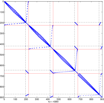
Fig. 2: An example of a 2-D Laplacian matrix which is partitioned into $4$ subdomains and reordered according to (5) (left) and (2) (right) respectively.

A popular way of solving a global system put into the form of (5) is to exploit the Schur complement techniques that eliminate the interior unknowns $u_{i}$ first and then focus on solving in some way for the interface unknowns. The interior unknowns can then be easily recovered by back substitution. Assuming that $B_{i}$ is nonsingular, $u_{i}$ in (2) can be eliminated by means of the first equation: $u_{i}=B_{i}^{-1}(f_{i}-E_{i}y_{i})$ which yields, upon substitution in (3),

$$S_{i}y_{i}+\sum_{j\in N_{i}}E_{ij}y_{j}=g_{i}-E_{i}^{T}B_{i}^{-1}f_{i}\equiv g^{\prime}_{i},$$ (6)

in which $S_{i}$ is the local Schur complement,

$$S_{i}=C_{i}-E_{i}^{T}B_{i}^{-1}E_{i}.$$

When written for each subdomain $i$, (6) yields the global Schur complement system that involves only the interface unknown vectors $y_{i}$ and the reduced system has a natural block structure,

$$\begin{pmatrix}S_{1}&E_{12}&\ldots&E_{1p}\cr E_{21}&S_{2}&\ldots&E_{2p}\cr\vdots&&\ddots&\vdots\cr E_{p1}&E_{p,2}&\ldots&S_{p}\end{pmatrix}\begin{pmatrix}y_{1}\cr y_{2}\cr\vdots\cr y_{p}\end{pmatrix}=\begin{pmatrix}g^{\prime}_{1}\cr g^{\prime}_{2}\cr\vdots\cr g^{\prime}_{p}\end{pmatrix}.$$ (7)

Each of the diagonal blocks in this system is the local Schur complement matrix $S_{i}$, which is dense in general. The off-diagonal blocks $E_{ij}$ are identical with those of the local system (4) and are sparse. A key idea here is to (approximately) solve the reduced system (7) efficiently. For example, in pARMS [29] efficient preconditioners are developed based on forming an approximation to the Schur complement system and then approximately solving (7) and then extracting the internal unknowns $u_{i}$. This defines a preconditioning operation for the global system. In the method proposed in this paper we do not try to solve the global Schur complement system or even form it. Instead, an approximate inverse preconditioner to the original matrix is obtained by exploiting a low-rank property and the SMW formula.

3 Domain decomposition with local low-rank corrections

The coefficient matrix of the system (5) is of the form

$$A\equiv\begin{pmatrix}B&\hat{E}\cr\hat{E}^{T}&C\end{pmatrix},$$ (8)

where $B\in\mathbb{R}^{m\times m}$, $\hat{E}\in\mathbb{R}^{m\times s}$ and $C\in\mathbb{R}^{s\times s}$. Here, we abuse notation by using the same symbol $A$ to represent the permuted version of the matrix in (1). The goal of this section is to build a preconditioner for the matrix (8).

3.1 Splitting

We begin by splitting matrix $A$ as follows

$$A=\begin{pmatrix}B&\hat{E}\cr\hat{E}^{T}&C\end{pmatrix}=\begin{pmatrix}B&\cr&C\end{pmatrix}+\begin{pmatrix}&\hat{E}\cr\hat{E}^{T}&\end{pmatrix},$$ (9)

and defining the $n\times s$ matrix,

$$E\equiv\begin{pmatrix}\alpha^{-1}\hat{E}\cr-\alpha I\end{pmatrix},$$ (10)

where $I$ is the $s\times s$ identity matrix and $\alpha$ is a parameter. Then from (9) we immediately get the identity,

$$\left[\begin{array}[]{c|c}B&\hat{E}\cr\hline\cr\hat{E}^{T}&C\end{array}\right]=\left[\begin{array}[]{c|c}B+\alpha^{-2}\hat{E}\hat{E}^{T}&0\cr\hline\cr 0&C+\alpha^{2}I\end{array}\right]-EE^{T}.$$ (11)

A remarkable property is that the operator $\hat{E}\hat{E}^{T}$ is local in that it does not involve inter-domain couplings. Specifically, we have the following proposition.

Proposition 1.

Consider the matrix $X=\hat{E}\hat{E}^{T}$ and its blocks $X_{ij}$ associated with the same blocking as for the matrix in (5). Then, for $1\leq i,j\leq p$ we have:

$$X_{ij} =0,\quad\mathrm{for}\quad i\neq j$$

$$X_{ii} =E_{i}E_{i}^{T}.$$

Proof.

This follows from the fact that the columns of $\hat{E}$ associated with different subdomains are structurally orthogonal illustrated on the left side of Figure 2. ∎

Thus, we can write

$$A=A_{0}-EE^{T},\quad A_{0}=\begin{pmatrix}B+\alpha^{-2}\hat{E}\hat{E}^{T}&\cr&C+\alpha^{2}I\end{pmatrix}\in\mathbb{R}^{n\times n},$$ (12)

with the matrix $E$ defined in (10). From (12) and the SMW formula, we can derive the expression for the inverse of $A$. First define,

$$G=I-E^{T}A_{0}^{-1}E.$$ (13)

Then, we have

$$A^{-1}=A_{0}^{-1}+A_{0}^{-1}E(\underbrace{I-E^{T}A_{0}^{-1}E}_{G})^{-1}E^{T}A_{0}^{-1}\equiv A_{0}^{-1}+A_{0}^{-1}EG^{-1}E^{T}A_{0}^{-1}.$$ (14)

Note that the matrix $C$ is often strongly diagonally dominant for matrices arising from the discretization of PDEs, and the parameter $\alpha$ can serve to improve diagonal dominance in the indefinite cases.

3.2 Low-rank approximation to the $\mathbf{G}$ matrix

In this section we will consider the case when $A$ is symmetric positive definite (SPD). A preconditioner of the form

$$M^{-1}=A_{0}^{-1}+(A_{0}^{-1}E)\tilde{G}^{-1}(E^{T}A_{0}^{-1})$$

can be readily obtained from (14) if we had an approximation $\tilde{G}^{-1}$ to $G^{-1}$. Note that the application of this preconditioner will involve two solves with $A_{0}$ instead of only one. It will also involve a solve with $\tilde{G}$ which operates on the interface unknowns. Let us, at least formally, assume that we know the spectral factorization of $E^{T}A_{0}^{-1}E$

$$H\equiv E^{T}A_{0}^{-1}E=U\Lambda U^{T},$$

where $H\in\mathbb{R}^{s\times s}$, $U$ is unitary, and $\Lambda$ is diagonal. From (12) we have $A_{0}=A+EE^{T}$, and thus $A_{0}$ is SPD since $A$ is SPD. Therefore, $H$ is at least symmetric positive semidefinite (SPSD) and the following lemma shows that its eigenvalues are all less than one.

Lemma 2.

Let $H=E^{T}A_{0}^{-1}E$. Assume that $A$ is SPD and the matrix $I-H$ is nonsingular. Then we have $0\leq\lambda<1$, for each eigenvalue $\lambda$ of $H$.

Proof.

From (14), we have

$$E^{T}A^{-1}E=H+H(I-H)^{-1}H=H\left(I+(I-H)^{-1}H\right)=H(I-H)^{-1}.$$

Since $A$ is SPD, $E^{T}A^{-1}E$ is at least SPSD. Thus, the eigenvalues of $H(I-H)^{-1}$ are nonnegative, i.e., $\lambda/(1-\lambda)\geq 0$. So, we have $0\leq\lambda<1$. ∎

The goal now is to see what happens if we replace $\Lambda$ by a diagonal matrix $\tilde{\Lambda}$. This will include the situation when a low-rank approximation is used for $G$ but it can also include other possibilities. Suppose that $H$ is approximated as follows:

$$H\approx U\tilde{\Lambda}U^{T}.$$ (15)

Then, from the SMW formula, the corresponding approximation to $G^{-1}$ is:

$$G^{-1}\approx\tilde{G}^{-1}\equiv(I-U\tilde{\Lambda}U^{T})^{-1}=I+U[(I-\tilde{\Lambda})^{-1}-I]U^{T}.$$ (16)

Note in passing that the above expression can be simplified to $U(I-\tilde{\Lambda})^{-1}U^{T}$. However, we keep the above form because it will still be valid when $U$ has only $k$ $(k<s)$ columns and $\tilde{\Lambda}$ is $k\times k$ diagonal, in which case we denote by $G_{k}^{-1}$ the approximation in (16). At the same time, the exact $G$ can be obtained as a special case of (16), where $\tilde{\Lambda}$ is simply equal to $\Lambda$. Then we have

$$A^{-1} =A_{0}^{-1}+(A_{0}^{-1}E)G^{-1}(E^{T}A_{0}^{-1}),$$ (17)

and the preconditioner

$$M^{-1} =A_{0}^{-1}+(A_{0}^{-1}E)G_{k}^{-1}(E^{T}A_{0}^{-1}),$$ (18)

from which it follows by subtraction that

$$A^{-1}-M^{-1}=(A_{0}^{-1}E)(G^{-1}-G_{k}^{-1})(E^{T}A_{0}^{-1}),$$

and therefore,

$$AM^{-1}=I-A(A_{0}^{-1}E)(G^{-1}-G_{k}^{-1})(E^{T}A_{0}^{-1}).$$ (19)

A first consequence of (19) is that there will be at lease $m$ eigenvalues of $AM^{-1}$ that are equal to one, where $m=n-s$ is the dimension of $B$ in (8) or in other words, the number of the interior unknowns. From (16) we obtain

$$G^{-1}-G_{k}^{-1}=U[(I-\Lambda)^{-1}-(I-\tilde{\Lambda})^{-1}]U^{T}.$$ (20)

The simplest selection of $\tilde{\Lambda}$ is the one that ensures that the $k$ largest eigenvalues of $(I-\tilde{\Lambda})^{-1}$ match the largest eigenvalues of $(I-\Lambda)^{-1}$. This simply minimizes the 2-norm of (20) under the assumption that the approximation in (15) is of rank $k$. Assume that the eigenvalues of $H$ are $\lambda_{1}\geq\lambda_{2}\geq\cdots\geq\lambda_{s}$. This means that the diagonal entries $\tilde{\lambda}_{i}$ of $\tilde{\Lambda}$ are selected such that

$$\tilde{\lambda}_{i}=\left\{\begin{array}[]{cl}\lambda_{i}&\mbox{if}\quad i\leq k\\ 0&\mbox{otherwise}\end{array}.\right.$$ (21)

Observe that from (20) the eigenvalues of $G^{-1}-G_{k}^{-1}$ are

$$\left\{\begin{array}[]{cl}0&\mbox{if}\quad i\leq k\\ (1-\lambda_{i})^{-1}-1&\mbox{otherwise}\end{array}.\right.$$

Thus, from (19) we can infer that $k$ more eigenvalues of $AM^{-1}$ will take the value one in addition to the existing $m$ ones revealed above independently of the choice of $\tilde{G}^{-1}$. Noting that $(1-\lambda_{i})^{-1}-1=\lambda_{i}/(1-\lambda_{i})\geq 0$, since $0\leq\lambda_{i}<1$ and we can say that the remaining $s-k$ eigenvalues of $AM^{-1}$ will be between $0$ and $1$. Therefore, the result in this case is that the preconditioned matrix $AM^{-1}$ in (19) will have $m+k$ eigenvalues equal to one, and $s-k$ other eigenvalues between 0 and 1.

From an implementation point of view, it is clear that a full diagonalization of $H$ is not needed. All we need is $U_{k}$, the $s\times k$ matrix consisting of the first $k$ columns of $U$, along with the diagonal matrix $\Lambda_{k}$ of the corresponding eigenvalues $\lambda_{1},\cdots,\lambda_{k}$. Then, noting that (16) is still valid with $U$ replaced by $U_{k}$ and $\Lambda$ replaced by $\Lambda_{k}$, we can get the approximation $G_{k}$ and its inverse directly:

$$G_{k}=I-U_{k}\Lambda_{k}U_{k}^{T},\quad G_{k}^{-1}=I+U_{k}[(I-\tilde{\Lambda}_{k})^{-1}-I]U_{k}^{T}.$$ (22)

It may have become clear to the reader that it is possible to select $\tilde{\Lambda}$ so that $AM^{-1}$ will have eigenvalues larger than one. Consider defining $\tilde{\Lambda}$ such that

$$\tilde{\lambda}_{i}=\left\{\begin{array}[]{cl}\lambda_{i}&\mbox{if}\quad i\leq k\\ \theta&\mbox{if}\quad i>k\\ \end{array},\right.$$

and denote by $G_{k,\theta}^{-1}$ the related analogue of (22). Then, from (20) the eigenvalues of $G^{-1}-G_{k,\theta}^{-1}$ are

$$\left\{\begin{array}[]{cl}0&\mbox{if}\quad i\leq k\\ (1-\lambda_{i})^{-1}-(1-\theta)^{-1}&\mbox{if}\quad i>k\\ \end{array}.\right.$$ (23)

Note that for $i>k$, we have

$$\frac{1}{1-\lambda_{i}}-\frac{1}{1-\theta}=\frac{\lambda_{i}-\theta}{(1-\lambda_{i})(1-\theta)},$$

and these eigenvalues can be made negative by selecting $\lambda_{k+1}\leq\theta<1$ and the choice that yields the smallest 2-norm is $\theta=\lambda_{k+1}$. The earlier definition of $\Lambda_{k}$ in (21) that truncates the eigenvalues of $H$ to zero corresponds to selecting $\theta=0$.

Theorem 3.

Assume that $A$ is SPD and $\theta$ is selected so that $\lambda_{k+1}\leq\theta<1$. Then the eigenvalues $\eta_{i}$ of $AM^{-1}$ are such that,

$$1\leq\eta_{i}\leq 1+\frac{1}{1-\theta}\ \|A^{1/2}A_{0}^{-1}E\|_{2}^{2}.$$ (24)

Furthermore, the term $\|A^{1/2}A_{0}^{-1}E\|_{2}^{2}$ is bounded from above by a constant:

$$\lVert A^{1/2}A_{0}^{-1}E\rVert_{2}^{2}\leq\frac{1}{4}.$$

Proof.

We rewrite (19) as $AM^{-1}=I+A(A_{0}^{-1}E)(G_{k}^{-1}-G^{-1})(E^{T}A_{0}^{-1})$ or upon applying a similarity transformation with $A^{1/2}$

$$A^{1/2}M^{-1}A^{1/2}=I+(A^{1/2}A_{0}^{-1}E)(G_{k}^{-1}-G^{-1})(E^{T}A_{0}^{-1}A^{1/2}).$$ (25)

From (23) we see that for $j\leq k$ we have $\lambda_{j}(G_{k}^{-1}-G^{-1})=0$, and for $j>k$,

$$0\leq\lambda_{j}(G_{k}^{-1}-G^{-1})=(1-\theta)^{-1}-(1-\lambda_{j})^{-1}\leq(1-\theta)^{-1}.$$

This is because $1/(1-t)$ is an increasing function and for $j>k$, we have $0\leq\lambda_{j}\leq\lambda_{k+1}\leq\theta$. The rest of the proof follows by taking the Rayleigh quotient of an arbitrary vector $x$ and utilizing (25).

For the second part, first note that $\lVert A^{1/2}A_{0}^{-1}E\rVert_{2}^{2}=\rho\left(E^{T}A_{0}^{-1}AA_{0}^{-1}E\right)$, where $\rho(\cdot)$ denotes the spectral radius of a matrix. Then, from $A=A_{0}-EE^{T}$, we have

$$E^{T}A_{0}^{-1}AA_{0}^{-1}E=E^{T}A_{0}^{-1}E-\left(E^{T}A_{0}^{-1}E\right)\left(E^{T}A_{0}^{-1}E\right)\equiv H-H^{2}.$$

Lemma 2 states that each eigenvalue $\lambda$ of $H$ satisfies $0\leq\lambda<1$. Hence, for each eigenvalue $\mu$ of $E^{T}A_{0}^{-1}AA_{0}^{-1}E$, $\mu=\lambda-\lambda^{2}$, which is between 0 and 1/4 for $\lambda\in\ [0,1)$. This gives the desired bound $\lVert A^{1/2}A_{0}^{-1}E\rVert_{2}^{2}\leq 1/4$. ∎

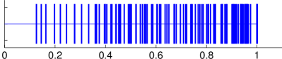
Fig. 3: DDLR-1: eigenvalues of $AM^{-1}$ with $\theta=0$ (left) and $\theta=\lambda_{k+1}$ (right) using $k=5$ eigenvectors for a $900\times 900$ 2-D Laplacian with $4$ subdomains and $\alpha=1$.

An illustration of the spectra of $AM^{-1}$ for the two cases when $\theta=0$ and $\theta=\lambda_{k+1}$ with $k=5$ is shown in Figure 3. The original matrix is a $900\times 900$ 2-D Laplacian obtained from a finite difference discretization of a square domain using $30$ mesh points in each direction. The number of the subdomains used is 4, resulting in 119 interface unknowns. The reordered matrix associated with this example were shown in Figure 2.

For the second choice $\theta=\lambda_{k+1}$, Theorem 3 proved that $\|A^{1/2}A_{0}^{-1}E\|_{2}^{2}$ does not exceed $1/4$, regardless of the mesh size and regardless of $\alpha$, Numerical experiments will show that this term is close to $1/4$ for Laplacian matrices. For the case with $\alpha=1$, $\theta=\lambda_{6}\approx 0.93492$ and $\lVert A^{1/2}A_{0}^{-1}E\rVert_{2}^{2}\approx 0.24996$, so that the bound of the eigenvalues of $AM^{-1}$ given by (24) is $4.8413$, which is fairly close to the largest eigenvalue, which is $4.3581$ (cf. the right part of Figure 3). When $\alpha=2$, $\theta=\lambda_{6}\approx 0.93987$ and $\lVert A^{1/2}A_{0}^{-1}E\rVert_{2}^{2}\approx 0.25000$, so that the eigenvalue bound is $5.1575$ whereas the largest eigenvalue is $4.6724$. When $\alpha=0.5$, $\theta=\lambda_{6}\approx 0.96945$ and $\lVert A^{1/2}A_{0}^{-1}E\rVert_{2}^{2}\approx 0.24999$, and thus the bound is $9.1840$, compared with the largest eigenvalue $8.6917$. Therefore, we conclude for this case $\alpha=1$ gives the best spectral condition number of the preconditioned matrix, which is a typical result for SPD matrices.

We now address some implementation issues of the preconditioner related to the second choice with $\theta=\lambda_{k+1}$. Again all that is needed are $U_{k}$, $\Lambda_{k}$ and $\theta$. We can show an analogue to the expression (22) in the following proposition.

Proposition 4.

The following expression for $G_{k,\theta}^{-1}$ holds:

$$G_{k,\theta}^{-1}=\frac{1}{1-\theta}I\ +\ U_{k}\left[(I-\Lambda_{k})^{-1}-(1-\theta)^{-1}I\right]U_{k}^{T}.$$ (26)

Proof.

We write $U=[U_{k},W]$, where $U_{k}$ is as before and $W$ contains the remaining columns $u_{k+1},\cdots,u_{s}$. Note that $W$ is not available but we use the fact that $WW^{T}=I-U_{k}U_{k}^{T}$ for the purpose of this proof. With this, (16) becomes:

$$G_{k,\theta}^{-1} =I+[U_{k},W]\begin{pmatrix}(I-\Lambda_{k})^{-1}-I&\\ &((1-\theta)^{-1}-1)I\end{pmatrix}[U_{k},W]^{T}$$

$$=I+U_{k}\left[(I-\Lambda_{k})^{-1}-I\right]U_{k}^{T}+\left[(1-\theta)^{-1}-1\right](I-U_{k}U_{k}^{T})$$

$$=\frac{1}{1-\theta}I\ +\ U_{k}\left[(I-\Lambda_{k})^{-1}-(1-\theta)^{-1}I\right]U_{k}^{T}.$$

∎

Proposition 5.

Let the assumptions of Lemma 2 be satisfied. The preconditioner (18) with the matrix $G_{k,\theta}^{-1}$ defined by (26) is well-defined and SPD when $\theta<1$.

Proof.

From (26), the eigenvalues of $G_{k,\theta}^{-1}$ are $(1-\lambda_{i})^{-1}$, $i=1,\ldots,k$ or $(1-\theta)^{-1}$. Recall from Lemma 2, $0\leq\lambda_{i}<1$ for all $i$ and thus $G_{k,\theta}^{-1}$ is well-defined and SPD when $\theta<1$. Hence, preconditioner (18) is SPD. ∎

We refer to the preconditioner (18) with $G_{k}^{-1}=G_{k,\theta}^{-1}$ as the one-sided DDLR preconditioner, abbreviated by DDLR-1.

3.3 Two-sided low-rank approximation

The method to be presented in this section uses low-rank approximations for more terms in (14), which yields a preconditioner that has a simpler form. Compared with the DDLR-1 method, the resulting preconditioner is less expensive to apply and less accurate in general. Suppose that $A_{0}^{-1}E\in\mathbb{R}^{n\times s}$ is factored in the form

$$A_{0}^{-1}E=UV^{T},$$ (27)

as obtained from the singular value decomposition (SVD), where $U\in\mathbb{R}^{n\times s}$ and $V\in\mathbb{R}^{s\times s}$ is orthogonal. Then, for the matrix $G$ in (13), we have the following lemma.

Lemma 6.

Let $G=I-E^{T}A_{0}^{-1}E$ as defined by (13) be nonsingular. Then,

$$G^{-1}=I+V\left(I-U^{T}EV\right)^{-1}U^{T}E.$$

Furthermore, the following relation holds,

$$V^{T}G^{-1}V=\left(I-U^{T}EV\right)^{-1}.$$ (28)

Proof.

For $G^{-1}$, we can write

$$G^{-1}=\left(I-(E^{T}A_{0}^{-1})E\right)^{-1}=\left(I-VU^{T}E\right)^{-1}=I+V\left(I-U^{T}EV\right)^{-1}U^{T}E.$$

Relation (28) follows from

$$V^{T}G^{-1}V =V^{T}(I+V\left(I-U^{T}EV\right)^{-1}U^{T}E)V=\left(I-U^{T}EV\right)^{-1}.$$

∎

From (27), the best $2$-norm rank-$k$ approximation to $A_{0}^{-1}E$ is of the form

$$A_{0}^{-1}E\approx U_{k}V_{k}^{T},$$ (29)

where $U_{k}\in\mathbb{R}^{n\times k}$ and $V_{k}\in\mathbb{R}^{s\times k}$ with $V_{k}^{T}V_{k}=I$ consist of the first $k$ columns of $U$ and $V$ respectively. For an approximation to $G$, we define the matrix $G_{k}$ as

$$G_{k}=I-V_{k}U_{k}^{T}E\ .$$ (30)

Then, the expression of $A^{-1}$ in (14) will yield the preconditioner:

$$M^{-1}=A_{0}^{-1}+U_{k}(V_{k}^{T}G_{k}^{-1}V_{k})U_{k}^{T}.$$

This means that we can build an approximate inverse based on a low-rank correction of the form that avoids the use of $V_{k}$ explicitly,

$$M^{-1}=A_{0}^{-1}+U_{k}H_{k}U_{k}^{T}\quad\mbox{with}\quad H_{k}=V_{k}^{T}G_{k}^{-1}V_{k}.$$ (31)

Note that Lemma 6 will also hold if $U$ and $V$ are replaced with $U_{k}$ and $V_{k}$. As a result, the matrix $H_{k}$ has an alternative expression that is more amenable to computation. Specifically, we can show the following lemma.

Lemma 7.

Let $G_{k}$ be defined by (30) and assume that matrix $I-U_{k}^{T}EV_{k}$ is nonsingular. Then,

$$G_{k}^{-1}=I+V_{k}\hat{H}_{k}U_{k}^{T}E\quad\mbox{with}\quad\hat{H}_{k}=(I-U_{k}^{T}EV_{k})^{-1}.$$

Furthermore, the following relation holds:

$$V_{k}^{T}G_{k}^{-1}V_{k}=\hat{H}_{k}$$

i.e., the matrix $H_{k}$ in (31) and the matrix $\hat{H}_{k}$ are equal.

Proof.

A proof can be directly obtained from the proof of Lemma 6 by replacing matrices $U$,$V$ and $G$ with $U_{k}$,$V_{k}$ and $G_{k}$ respectively. ∎

The application of (31) requires one solve with $A_{0}$ and a low-rank correction with $U_{k}$ and $H_{k}$. Since $A_{0}^{-1}E$ is approximated on both sides of $G$ in (14), we refer to this preconditioner as a two-sided DDLR preconditioner and use the abbreviation DDLR-2.

Proposition 8.

Assume that $U_{k}V_{k}^{T}$ in (29) is the best $2$-norm rank-$k$ approximation to $A_{0}^{-1}E$, and that $A_{0}$ is SPD. Then the preconditioner given by (31) is well-defined and SPD if and only if $\rho(U_{k}^{T}EV_{k})<1$.

Proof.

The proof follows from Proposition 3.2 in [27] showing the symmetry of $H_{k}$, and Proposition 3.4 and Theorem 3.6 in [27] for the if-and-only-if condition. ∎

Next, we will show that the eigenvalues of the preconditioned matrix $AM^{-1}$ are between zero and one. Suppose that $U_{k}V_{k}^{T}$ is obtained as in (29), so that we have $\left(A_{0}^{-1}E\right)V_{k}=U_{k}$. Then, the preconditioner (31) can be rewritten as

$$M^{-1} =A_{0}^{-1}+U_{k}H_{k}U_{k}^{T}=A_{0}^{-1}+\left(A_{0}^{-1}E\right)V_{k}H_{k}V_{k}^{T}\left(E^{T}A_{0}^{-1}\right)$$

$$=A_{0}^{-1}+\left(A_{0}^{-1}E\right)V\begin{pmatrix}H_{k}&0\\ 0&0\end{pmatrix}V^{T}\left(E^{T}A_{0}^{-1}\right),$$ (32)

where $U$ and $V$ are defined in (27). We write $U=\left[U_{k},\bar{U}\right]$ and $V=\left[V_{k},\bar{V}\right]$, where $\bar{U}$ and $\bar{V}$ consist of the $s-k$ columns of $U$ and $V$ that are not contained in $U_{k}$ and $V_{k}$. Recall that $H_{k}^{-1}=I-U_{k}^{T}EV_{k}$ and define $X=I-\bar{U}^{T}E\bar{V}$, $Z=-U_{k}^{T}E\bar{V}$. From (17) and (27), we have

$$A^{-1}=A_{0}^{-1}+\left(A_{0}^{-1}E\right)V\left(V^{T}G^{-1}V\right)V^{T}\left(E^{T}A_{0}^{-1}\right),$$

from which and (28), it follows that

$$A^{-1} =A_{0}^{-1}+\left(A_{0}^{-1}E\right)V\left(I-U^{T}EV\right)^{-1}V^{T}\left(E^{T}A_{0}^{-1}\right),$$

$$=A_{0}^{-1}+\left(A_{0}^{-1}E\right)V\begin{pmatrix}H_{k}^{-1}&Z\\ Z^{T}&X\end{pmatrix}^{-1}V^{T}\left(E^{T}A_{0}^{-1}\right).$$ (33)

Let the Schur complement of $H_{k}^{-1}$ be

$$S_{k}=X-Z^{T}H_{k}Z\in\mathbb{R}^{(s-k)\times(s-k)},$$ (34)

and define matrix $\bar{S}_{k}\in\mathbb{R}^{2(s-k)\times 2(s-k)}$ by

$$\bar{S}_{k}=\begin{pmatrix}S_{k}^{-1}&-I\\ -I&S_{k}\end{pmatrix}.$$ (35)

Then, the following lemma shows that $S_{k}$ is SPD and $\bar{S}_{k}$ is SPSD.

Lemma 9.

Assume that $G$ defined by (14) is nonsingular as well as the matrix $I-U_{k}^{T}EV_{k}$. Then, the Schur complement $S_{k}$ defined by (34) is SPD. Moreover, matrix $\bar{S}_{k}$ is SPSD with $s-k$ positive eigenvalues and $s-k$ zero eigenvalues.

Proof.

From Lemma 2, we can infer that the eigenvalues of $G$ are all positive. Thus, $G$ is SPD and so is matrix $V^{T}G^{-1}V$. In the end, the Schur complement $S_{k}$ is SPD when $H_{k}$ is nonsingular. The signs of the eigenvalues of $\bar{S}_{k}$ can be easy revealed by a block LDL factorization. ∎

Theorem 10.

Assume that $A$ is SPD. Then the eigenvalues $\eta_{i}$ of $AM^{-1}$ with $M^{-1}$ given by (31) satisfy $0<\eta_{i}\leq 1$.

Proof.

From (3.3) and (3.3), it follows by subtraction that

$$A^{-1}-M^{-1} =\left(A_{0}^{-1}E\right)V\left[\begin{pmatrix}H_{k}^{-1}&Z\\ Z^{T}&X\end{pmatrix}^{-1}-\begin{pmatrix}H_{k}&0\\ 0&0\end{pmatrix}\right]V^{T}\left(E^{T}A_{0}^{-1}\right),$$

$$=\left(A_{0}^{-1}E\right)V\begin{pmatrix}H_{k}ZS_{k}^{-1}Z^{T}H_{k}&-H_{k}ZS_{k}^{-1}\\ -S_{k}^{-1}Z^{T}H_{k}&S_{k}^{-1}\end{pmatrix}V^{T}\left(E^{T}A_{0}^{-1}\right),$$

$$=\left(A_{0}^{-1}E\right)V\begin{pmatrix}H_{k}Z&0\\ 0&S_{k}^{-1}\end{pmatrix}\bar{S}_{k}\begin{pmatrix}Z^{T}H_{k}&0\\ 0&S_{k}^{-1}\end{pmatrix}V^{T}\left(E^{T}A_{0}^{-1}\right),$$

where $\bar{S}_{k}$ is defined in (35), so that

$$AM^{-1}=I-A\left(A_{0}^{-1}E\right)V\begin{pmatrix}H_{k}Z&0\\ 0&S_{k}^{-1}\end{pmatrix}\bar{S}_{k}\begin{pmatrix}Z^{T}H_{k}&0\\ 0&S_{k}^{-1}\end{pmatrix}V^{T}\left(E^{T}A_{0}^{-1}\right).$$

Hence, the eigenvalues of $AM^{-1}$, $\eta_{i}$, satisfy $0<\eta_{i}\leq 1$, since $\bar{S}_{k}$ is SPSD, and $(n-s+k)$ of these eigenvalues are equal to one. ∎

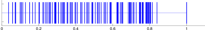
Fig. 4: DDLR-2: eigenvalues of $AM^{-1}$ with $k=5$ eigenvectors for a $900\times 900$ 2-D Laplacian with $4$ subdomains and $\alpha=1$.

The spectrum of $AM^{-1}$ for the same matrix used for Figure 3 is shown in Figure 4. Compared with the spectrum with the DDLR-1 method with $\theta=0$ shown in the left part of Figure 3, the eigenvalues of the preconditioned matrix $AM^{-1}$ are more dispersed between 0 and 1 and the small eigenvalues are closer to zero. This suggests that the quality of the DDLR-2 preconditioner will be lower than that of DDLR-1, which is supported by the numerical results in Section 5.

4 Implementation

In this section, we address the implementation details for building and applying the DDLR preconditioner, especially focusing on the implementations in a parallel/distributed environment.

4.1 Building a DDLR preconditioner

The construction of a DDLR preconditioner involves the following steps. In the first step, a graph partitioner is called on the adjacency graph to partition the domain. For each obtained subdomain, we separate the interior nodes and the interface nodes, and reorder the local matrix into the form of (2). The second step is to build a solver for each $B_{i,\alpha}\equiv B_{i}+\alpha^{-2}E_{i}E_{i}^{T}$. These two steps can be done in parallel. The third step is to build a solver for the global matrix $C_{\alpha}$. We will focus on the solution methods for the linear systems with $C_{\alpha}$ in Section 4.3. The last step, which is the most expensive one, is to compute the low-rank approximations. This will be discussed in Section 4.4.

4.2 Applying the DDLR preconditioner

First, consider the DDLR-1 preconditioner (18), which we can rewrite as

$$M^{-1}=A_{0}^{-1}\left(I+EG_{k,\theta}^{-1}E^{T}A_{0}^{-1}\right).$$ (36)

The steps involved in applying $M^{-1}$ to a vector $x$ are listed in Algorithm 1. The vector $u$ resulting from the last step will be the desired vector $u=M^{-1}x$. The solve with $A_{0}$ required in steps 1 and 5 of Algorithm 1, can in turn be viewed as consisting of the $p$ independent local solves with $B_{i,\alpha}$ and the global solve with $C_{\alpha}\equiv C+\alpha^{2}I$ as is inferred from (12). Recall that the matrix $C$, which has the block structure (4), is the global interface matrix that couples all the interface unknowns. So, solving a linear system with $C_{\alpha}$ will require communication if $C_{\alpha}$ is assigned to different processors. The multiplication with $E^{T}$ in step 2 transforms a vector of the interior unknowns into a vector of the interface unknowns. This can be likened to a descent operation that moves objects from a “fine” space to a “coarse” space. The multiplication with $E$ in step 4 performs the reverse operation, which can be termed an ascent operation, consisting of going from the interface unknowns to the interior unknowns. Finally, the operation with $G_{k,\theta}^{-1}$ in step 3 involves all the interface unknowns, and it will also require communication. In summary, there are essentially 4 types of operations: (1) the solve with $B_{i,\alpha}$; (2) the solve with $C_{\alpha}$; (3) products with $E$ and $E^{T}$, which are dual of one another; and (4) the application of $G_{k,\theta}^{-1}$ to vectors.

Algorithm 1 Preconditioning operations of the DDLR-1 preconditioner.

1:  Solve: $A_{0}z=x$ {$B_{i,\alpha}$ solves and $C_{\alpha}$ solve}

2:  Compute: $y=E^{T}z$ {Interior unknowns to interface neighbors}

3:  Compute: $w=G_{k,\theta}^{-1}y$ {Use (26)}

4:  Compute: $v=Ew$ {Interface unknowns to interior neighbors}

5:  Solve: $A_{0}u=x+v$ {$B_{i,\alpha}$ solves and $C_{\alpha}$ solve}

Next, consider the DDLR-2 preconditioner given by (31). Applying this preconditioner is much simpler, which consists of one solve with $A_{0}$ and a low-rank correction. Communication will be required for applying the low-rank correction term, $U_{k}H_{k}U_{k}^{T}$, to a vector because it involves all the unknowns. We assume that the $k\times k$ matrix $H_{k}$ is stored on every processor.

Parallel implementations of the DDLR methods will depend on how the interface unknowns are mapped to processors. A few of the mapping schemes will be discussed in Section 4.5.

4.3 The global solves with $\mathbf{C_{\alpha}}$

This section addresses the solution methods for $C_{\alpha}$ required in both the DDLR-1 and the DDLR-2 methods whenever solving a linear system with $A_{0}$ is needed. It is an important part of the computations, especially for DDLR-1 as it takes place twice for each iteration. In addition, it is a non-local computation and can be costly due to the communication. An important characteristic of $C_{\alpha}$ is that it can be made strongly diagonally dominant by selecting a proper scaling factor $\alpha$. Therefore, the first approach one can think about is to use a few steps of the Chebyshev iterations. The Chebyshev method was used with a block Jacobi preconditioner $D_{\alpha}$ consisting of all the local diagonal blocks $C_{i}$ (see, e.g., [6, §2.3.9] for the preconditioned Chebyshev method). An appealing property in the Chebyshev iterations is that no inner product is needed. This avoids communications among processors, which makes this method efficient in particular for distributed memory architectures [35]. The price one pays for avoiding communication is that this method requires enough knowledge of the spectrum. Therefore, prior to the Chebyshev iterations, we performed a few steps of the Lanczos iterations on the matrix pair $(C_{\alpha},D_{\alpha})$ [36, §9.2.6] for some estimates (not bounds) of the smallest and the largest eigenvalues. The safeguard terms used in [43] were included in order to have bounds of the spectrum (see [30, §13.2] for the definitions of these terms).

Another approach is to resort to an approximate inverse $X\approx C_{\alpha}^{-1}$, so that the solve with $C_{\alpha}$ will be reduced to a matrix vector product with $X$. A simple scheme known as the method of Hotelling and Bodewig [20] is given by the iteration

$$X_{k+1}=X_{k}(2I-C_{\alpha}X_{k}).$$

In the absence of dropping, this scheme squares the residual norm $\lVert I-C_{\alpha}X_{k}\rVert$ from one step to the next, so that it converges quadratically provided that the initial guess $X_{0}$ is such that $\|I-C_{\alpha}X_{0}\|<1$ for some matrix norm. The global self-preconditioned minimal residual (MR) iterations were shown to have superior performance [10]. We adopted this method to build an approximate inverse of $C_{\alpha}$. Given an initial guess $X_{0}$, the self-preconditioned MR iterations can be obtained by the sequence of operations shown in Algorithm 2. $X_{0}$ was selected as the inverse of the diagonal of $C_{\alpha}$. The numerical dropping was performed by a dual threshold strategy based on a drop tolerance and a maximum number of nonzeros per column.

Algorithm 2 Self-preconditioned global MR iterations with dropping.

1:  Compute: $R_{k}=I-C_{\alpha}X_{k}$ {residual}

2:  Compute: $Z_{k}=X_{k}R_{k}$ {self-preconditioned residual}

3:  Apply numerical dropping to $Z_{k}$

4:  Compute: $\beta_{k}=\mathrm{tr}(R_{k}^{T}C_{\alpha}Z_{k})/\left\|C_{\alpha}Z_{k}\right\|_{F}^{2}$ {tr$(\cdot)$ denotes the trace}

5:  Compute: $X_{k+1}=X_{k}+\beta_{k}Z_{k}$

4.4 Computation of low-rank approximations

For the DDLR-1 method, we use the Lanczos algorithm [24] to compute the low-rank approximation to $E^{T}A_{0}^{-1}E$ that is of the form $U_{k}\Lambda_{k}U_{k}^{T}$. For the DDLR-2 method, the low-rank approximation to $A_{0}^{-1}E$ is of the form $U_{k}V_{k}^{T}$, which can be computed by applying the Lanczos algorithm on $E^{T}A_{0}^{-2}E$, where $V_{k}$ is computed and $U_{k}$ can be obtained by $U_{k}=A_{0}^{-1}EV_{k}$. Alternatively, for the DDLR-2 method, we can also use the Lanczos bidiagonalization method [17, §10.4] to compute $U_{k}$ and $V_{k}$ at the same time. At each step of the Lanczos algorithm, a matrix-vector product is required. This means that for each step, we need to solve linear systems with $A_{0}$: one solve for the DDLR-1 method and two for the DDLR-2 method.

As is well-known, in the presence of rounding error, orthogonality in the Lanczos procedure is quickly lost and a form of reorthogonalization is needed in practice. In our approach, the partial reorthogonalization scheme [31, 39] is used. The cost of this step will not be an issue to the overall performance when a small number of steps are performed to approximate a few eigenpairs. To monitor convergence of the computed eigenvalues, we adopt the approach used in [16]. Let $\theta_{j}^{(m-1)}$ and $\theta_{j}^{(m)}$ be the Ritz values obtained in two consecutive Lanczos steps, $m-1$ and $m$. Assume that we want to approximate $k$ largest eigenvalues and $k<m$. Then with a preselected tolerance $\epsilon$, the desired eigenvalues are considered to have converged if

$$\left|\frac{\sigma_{m}-\sigma_{m-1}}{\sigma_{m-1}}\right|<\epsilon,\textrm{ where }\sigma_{m-1}={\displaystyle\sum_{j=1}^{k}\theta_{j}^{(m-1)}}\textrm{ and }\sigma_{m}={\displaystyle\sum_{j=1}^{k}\theta_{j}^{(m)}}.$$ (37)

4.5 Parallel implementations: standard mapping

Considerations of the parallel implementations have been mentioned in the previous sections, which suggest several possible schemes for distributing the interface unknowns. Before discussing these schemes, it will be helpful to overview the issues at hand. Major computations in building and applying the DDLR preconditioners are the following:

1. solve with $B_{i,\alpha}$, (local)

2. solve with $C_{\alpha}$, (nonlocal)

3. products with $E^{T}$ and $E$, (local)

4. for DDLR-1, applying $G_{k,\theta}^{-1}$ in (26), (nonlocal)

5. for DDLR-2, products with $U_{k}$ and $U_{k}^{T}$, (nonlocal)

6. reorthogonalizations in the Lanczos procedure. (nonlocal)

The most straightforward mapping we can consider might be to map the unknowns of each subdomain to a processor. If $p$ subdomains are used, global matrices $A$ and $C_{\alpha}$ or its approximate inverse $X$ are distributed among the $p$ processors. So, processor $i$ will hold $d_{i}+s_{i}$ rows of $A$ and $s_{i}$ rows of $C_{\alpha}$ or $X$, where $d_{i}$ is the number of the local interior unknowns and $s_{i}$ is the number of the local interface unknowns of subdomain $i$. In the DDLR-1 method, $U_{k}\in\mathbb{R}^{s\times k}$ is distributed such that processor $i$ will keep $s_{i}$ rows, while in the DDLR-2 method, $d_{i}+s_{i}$ rows of $U_{k}\in\mathbb{R}^{n\times k}$ will reside in processor $i$. For all the nonlocal operations, communication is among all the $p$ processors. The operations labeled by (2.) and (4a.) involve interface to interface communication, while the operations (4b.) and (5.) involve communication among all the unknowns. From another perspective, the communication in (4a.), (4b.) and (5.) is of the all-reduction type required by vector inner products, while the communication in (2.) is point-to-point such as that in the distributed sparse matrix vector products. If an iterative process is used for the solve with $C_{\alpha}$, it is important to select $\alpha$ carefully so as to reach a compromise between the number of the inner iterations (each of which requires communication) and the number of the outer iterations (each of which involves solves with $C_{\alpha}$). The scalar $\alpha$ will also play a role if an approximate inverse is used, since the convergence of the MR iterations will be affected.

4.6 Unbalanced mapping: interface unknowns together

Since communication is required among the interface nodes, an idea that comes to mind is to map the interior unknowns of each subdomain to a processor, and all the interface unknowns to another separated one. In a case of $p$ subdomains, $p+1$ processors will be used and $A$ is distributed in such a way that processor $i$ owns the rows corresponding to the local interior unknowns for $i=1,\ldots p$, while processor $p+1$ holds the rows related to all the interface unknowns. Thus, $C_{\alpha}$ or $X$ will reside entirely on the processor $p+1$.

A clear advantage of this mapping is that the solve with $C_{\alpha}$ will require no communication. However, the operations with $E$ and $E^{T}$ are no longer local. Indeed, $E^{T}$ can be viewed as a restriction operator, which “scatters” interface data from processor $p+1$ to the other $p$ processors. Specifically, referring to (2), each $y_{i}$ will be sent to processor $i$ from processor $p+1$. Analogously, the product with $E$, as a prolongation, will perform a dual operation that “gathers” from processors $1$ to $p$ to processor $p+1$. In Algorithm 1, the scatter operation goes before step $2$ and the gather operation should be executed after step $4$. Likewise, if we store the vectors in $U_{k}$ on processor $p+1$, applying $G_{k,\theta}$ will not require communication but another pair of the “gather-and-scatter” operations will be needed before and after step 3. Therefore, at each application of the DDLR-1 preconditioner, two pairs of the scatter-and-gather operations for the interface unknowns will be required. A middle ground approach is to distribute $U_{k}$ to processors $1$ to $p$ as it is in the standard mapping. In this way, applying $G_{k,\theta}$ will require communication but only one pair of the scatter-and-gather operations is necessary. On the other hand, in the DDLR-2 method, the distribution of $U_{k}$ should be consistent with that of $A$.

The main issue with this mapping is that it is hard to achieve load balancing in general. Indeed for a good balancing, we need to have the interior unknowns of each subdomain and all the interface unknowns of roughly the same size. However, this is difficult to achieve in practice. The load balancing issue is further complicated by the fact that the equations needed to be solved on processor $p+1$ are completely different from those on the other processors. A remedy to the load balancing issue is to use $q$ processors instead of just one dedicated to the global interface (a total of $p+q$ processors used in all), which provides a compromise. Then, the communication required for solving with $C_{\alpha}$ and applying $G_{k,\theta}$ is confined within the $q$ processors.

4.7 Improving a given preconditioner

One of the main weaknesses of standard, e.g., ILU-type, preconditioners is that they are difficult to update. For example, suppose we compute a preconditioner to a given matrix and find that it is not accurate enough to yield convergence. In the case of ILU we would have essentially to start from the beginning. For DDLR, improving a given preconditioner is essentially trivial. For example, the heart of DDLR-1 consists of obtaining a low-rank approximation the matrix $G$ defined in (13). Improving this approximation would consist in merely adding a few more vectors (increasing $k$) and this can be easily achieved in a number of ways without having to throw away the vectors already computed.

5 Numerical experiments

The experiments were conducted on Itasca, an HP ProLiant BL280c G6 Linux cluster at Minnesota Supercomputing Institute, which has $2,186$ Intel Xeon X5560 processors. Each processor has four cores, 8 MB cache, and communicates with memory on a QuickPath Interconnect (QPI) interface. An implementation of the DDLR preconditioners was written in C/C++ with the Intel Math Kernel Library, the Intel MPI library and PETSc [3, 4, 5], compiled by the Intel MPI compiler using the -O3 optimization level.

The accelerators used were the conjugate gradient (CG) method when both the matrix and the preconditioner are SPD, and the generalized minimal residual (GMRES) method with a restart dimension of $40$, denoted by GMRES$(40)$, for the indefinite cases. Three types of preconditioners were compared in our experiments: 1) the DDLR preconditioners, 2) the pARMS method [29], and 3) the RAS preconditioner [8] (with overlapping). Recall that for an SPD matrix, the DDLR preconditioners given by (18) and (31) will also be SPD if the assumptions in Propositions 5 and 8 are satisfied. However, these propositions will not hold when the solves with $A_{0}$ are approximate, which is typical in practice. Instead, the positive definiteness can be determined by checking if the largest eigenvalue is less than one for DDLR-1 or by checking the positive definiteness of $H_{k}$ for DDLR-2. DDLR-1 was always used with $\theta=\lambda_{k+1}$.

Each $B_{i,\alpha}$ was reordered by the approximate minimum degree ordering (AMD) [1, 2, 11] to reduce fill-ins and then we simply used an incomplete Cholesky or LDL factorization as the local solver. A more efficient and robust local solver, for example, the ARMS approach in [38], can lead to better performance in terms of both the memory requirement and the speed. However, this has not been implemented in our current code. A typical setting of the scalar $\alpha$ for $C_{\alpha}$ and $B_{i,\alpha}$ is $\alpha=1$, which in general gives the best overall performance, the exceptions being the three cases shown in Section 5.2, for which choosing $\alpha>1$ improved the convergence. Regarding the solves with $C_{\alpha}$, using the approximate inverse is generally more efficient than the Chebyshev iterations, especially in the iteration phase. However, computing the approximate inverse can be costly, in particular for the indefinite 3-D cases. The standard mapping was adopted unless specially stated, which in general gave better performance than the unbalanced mapping. The behavior of these two types of mappings will be analyzed by the results in Table 3. In the Lanczos algorithm, the convergence was checked every $10$ iterations and the tolerance $\epsilon$ in (37) used for the checking was $10^{-4}$. In addition, the maximum number of the Lanczos steps was five times the number of the requested eigenvalues.

For pARMS, the ARMS method was used to be the local preconditioner and the Schur complement method was used as the global preconditioner, where the reduced system was solved by a few inner Krylov subspace iterations preconditioned by the block-Jacobi preconditioner. For the details of these options in pARMS, we refer the readers to [37, 38]. We point out that when the inner iterations are enabled, flexible Krylov subspace methods will be required for the outer iterations, since the preconditioning is no longer fixed from one outer iteration to the next. So, the flexible GMRES [34] was used. For the RAS method, ILU($k$) was used as the local solver, and a one-level overlapping between subdomains was used. Note that the RAS preconditioner is nonsymmetric even for a symmetric matrix, so that GMRES was used with it.

We first report on the results of solving the linear systems from a 2-D and a 3-D PDEs on regular meshes. Next, we will show the results for solving a sequence of general sparse symmetric linear systems. For all the problems, a parallel multilevel $k$-way graph partitioning algorithm from ParMetis [21, 22] was used for the DD. Iterations were stopped whenever the residual norm had been reduced by $6$ orders of magnitude or the maximum number of iterations allowed, which is $500$, was exceeded. The results are shown in Tables 1, 2 and 5, where all timings are reported in seconds and ‘F’ indicates non-convergence within the maximum allowed number of steps. When comparing the preconditioners, the following factors are considered: 1) fill-ratio, i.e., the ratio of the number of nonzeros required to store a preconditioner to the number of nonzeros in the original matrix, 2) time for building preconditioners, 3) the number of iterations and 4) time for the iterations.

5.1 Model problems

We examine a 2-D and a 3-D PDE,

$$-\Delta u-cu =f\>\textrm{ in }\Omega,$$

$$u =0\textrm{ on }\partial\Omega,$$ (38)

where $\Omega=\left(0,1\right)^{2}$ or $\Omega=\left(0,1\right)^{3}$, and $\partial\Omega$ is the boundary. We take the $5$-point (or $7$-point) centered difference approximation. To begin with, we solve (5.1) with $c=0$. The matrix is SPD, so that we use DDLR with CG. Numerical experiments were carried out to compare the performance of DDLR with those of pARMS and RAS. The results are shown in Table 1. The mesh sizes, the number of processors (Np), the rank (rk), the fill-ratios (nz), the numbers of iterations (its), the time for building the preconditioners (p-t) and the time for iterations (i-t) are tabulated. We tested the problems on 6 2-D and 6 3-D meshes of increasing sizes, where the number of processors was growing proportionally such that the problem size on each processor was kept roughly the same. This can serve as a weak scaling test. We increased the rank $k$ used in DDLR with the meshes sizes. The fill-ratios of DDLR-1 and pARMS were controlled to be roughly equal, whereas the fill of DDLR-2 was much higher, which comes mostly from the matrix $U_{k}$ when $k$ is large. For pARMS, the inner Krylov subspace dimension used was $3$.

The time for building DDLR is much higher and it grows with the rank and the number of the processors. In contrast, the time to build pARMS and RAS is roughly constant. This set-up time for DDLR is typically dominated by the Lanczos algorithm, where solves with $B_{i,\alpha}$ and $C_{\alpha}$ are required at each iteration. Moreover, when $k$ is large, the cost of reorthogonalization becomes significant. As shown in Table 1, DDLR-1 and pARMS were more robust as they succeeded for all the 2-D and 3-D cases, while DDLR-2 failed for the largest 2-D case and RAS failed for the three largest ones. For most of the 2-D problems, DDLR-1/CG achieved convergence in the fewest iterations and the best iteration time. For the 3-D problems, DDLR-1 required more iterations but a performance gain was still achieved in terms of the reduced iteration time. Exceptions were the two largest 3-D problems, where RAS/GMRES yielded the best iteration time.

Table 1: Comparison between DDLR, pARMS and RAS preconditioners for solving SPD linear systems from the 2-D/3-D PDE with the CG or GMRES(40) method.

Mesh	Np	DDLR-1					DDLR-2
		rk	nz	its	p-t	i-t	rk	nz	its	p-t	i-t
$128^{2}$	2	8	6.6	15	.209	.027	8	8.2	30	.213	.031
$256^{2}$	8	16	6.6	34	.325	.064	16	9.7	69	.330	.083
$512^{2}$	32	32	6.8	61	.567	.122	32	13.0	132	.540	.194
$1024^{2}$	128	64	7.0	103	1.12	.218	64	19.3	269	1.03	.570
$1448^{2}$	256	91	7.2	120	1.67	.269	91	24.7	385	1.72	1.05
$2048^{2}$	512	128	7.6	168	3.02	.410	128	32.2	F	-	-
$25^{3}$	2	8	7.2	11	.309	.025	8	8.3	17	.355	.021
$50^{3}$	16	16	7.5	27	.939	.064	16	9.3	52	.958	.076
$64^{3}$	32	16	7.4	36	1.06	.089	16	9.2	67	1.07	.102
$100^{3}$	128	32	8.0	52	1.57	.136	32	11.5	101	1.48	.190
$126^{3}$	256	32	8.2	65	2.07	.178	32	12.5	126	1.87	.265
$159^{3}$	512	51	8.7	85	2.92	.251	51	14.2	156	2.50	.387

Mesh	Np	pARMS					RAS
			nz	its	p-t	i-t		nz	its	p-t	i-t
$128^{2}$	2		6.7	15	.062	.037		12.7	40	.003	.032
$256^{2}$	8		6.7	30	.066	.082		12.7	102	.004	.072
$512^{2}$	32		6.9	52	.072	.194		12.7	212	.005	.157
$1024^{2}$	128		6.6	104	.100	.359		12.7	F	.008	-
$1448^{2}$	256		6.6	247	.073	.820		12.7	F	.011	-
$2048^{2}$	512		6.8	282	.080	1.06		12.7	F	.015	-
$25^{3}$	2		7.3	9	.100	.032		15.9	13	.004	.041
$50^{3}$	16		8.1	17	.179	.095		16.7	28	.006	.071
$64^{3}$	32		8.2	20	.142	.121		16.7	34	.007	.103
$100^{3}$	128		8.3	29	.170	.198		16.7	51	.011	.148
$126^{3}$	256		8.4	34	.166	.216		16.7	60	.014	.127
$159^{3}$	512		8.5	40	.179	.275		16.7	83	.019	.183

Next, we consider solving symmetric indefinite problems by setting $c>0$ in (5.1), which corresponds to shifting the discretized negative Laplacian by subtracting $\sigma I$ with a certain $\sigma>0$. In this set of experiments, we reduce the size of the shift as the problem size increases in order to make the problems fairly difficult but not too difficult to solve for all the methods. We used higher ranks in the two DDLR methods and a higher inner iteration number, which was $6$, in pARMS. Results are reported in Table 2. From there we can see that DDLR-2 did not perform well as it failed for almost all the problems. Second, RAS failed for all the 2-D cases and three 3-D cases. But for the three cases where it worked, it yielded the best iteration time. Third, DDLR-1 achieved convergence in all the cases whereas pARMS failed for two 2-D cases. Comparison between DDLR-1 and pARMS shows a similar result as in the previous set of experiments: for the 2-D cases, DDLR-1 required fewer iteration and less iteration time, while for the 3-D cases, it might require more iterations but still less iteration time.

Table 2: Comparison between DDLR, pARMS and RAS preconditioners for solving symmetric indefinite linear systems from the 2-D/3-D PDEs with the GMRES(40) method.

Mesh	Np	$\sigma$	DDLR-1					DDLR-2
			rk	nz	its	p-t	i-t	rk	nz	its	p-t	i-t
$128^{2}$	2	1e-1	16	6.8	18	.233	.034	16	13.2	146	.310	.234
$256^{2}$	8	1e-2	32	6.8	38	.674	.080	16	13.0	F	1.01	-
$512^{2}$	32	1e-3	64	7.1	48	1.58	.105	64	19.4	F	1.32	-
$1024^{2}$	128	2e-4	128	7.6	68	4.15	.160	128	32.3	F	4.45	-
$1448^{2}$	256	5e-5	182	8.1	100	7.14	.253	182	43.2	F	7.77	-
$2048^{2}$	512	2e-5	256	8.8	274	12.6	.749	256	58.4	F	13.1	-
$25^{3}$	2	.25	16	8.3	29	.496	.099	16	9.6	62	.595	.130
$50^{3}$	16	7e-2	32	8.2	392	1.38	1.19	32	10.2	F	1.66	-
$64^{3}$	32	3e-2	64	8.9	201	2.26	.688	64	16.3	F	2.08	-
$100^{3}$	128	2e-2	128	11.4	279	5.17	1.08	128	28.7	F	5.29	-
$126^{3}$	256	7e-3	128	12.8	255	5.85	1.10	128	28.3	F	6.01	-
$159^{3}$	512	5e-3	160	13.5	387	8.60	1.71	160	33.0	F	8.33	-

Mesh	Np	$\sigma$	pARMS					RAS
				nz	its	p-t	i-t		nz	its	p-t	i-t
$128^{2}$	2	1e-1		11.4	76	.114	.328		12.7	F	.003	-
$256^{2}$	8	1e-2		13.9	F	-	-		12.7	F	.004	-
$512^{2}$	32	1e-3		12.3	298	.181	1.53		12.7	F	.005	-
$1024^{2}$	128	2e-4		12.5	232	.230	1.46		12.7	F	.008	-
$1448^{2}$	256	5e-5		12.5	F	-	-		12.7	F	.011	-
$2048^{2}$	512	2e-5		12.6	314	.195	2.13		12.7	F	.015	-
$25^{3}$	2	.25		8.3	100	.156	.599		15.9	108	.004	.123
$50^{3}$	16	7e-2		8.9	448	.142	2.59		16.7	F	.006	-
$64^{3}$	32	3e-2		8.9	130	.115	.784		16.7	252	.007	.375
$100^{3}$	128	2e-2		9.4	187	.137	1.24		16.7	343	.011	.541
$126^{3}$	256	7e-3		10.6	340	.137	2.74		16.7	F	.014	-
$159^{3}$	512	5e-3		10.8	329	.148	2.85		16.7	F	.019	-

In all the previous tests, DDLR-1 was used with the standard mapping. In the next set of experiments, we examined the behavior of the unbalanced mapping discussed in Section 4.6. In these experiments, we tested the problem on a $128\times 128$ mesh and a $25\times 25\times 25$ mesh. Both of them were divided into $128$ subdomains. Note here that the problem size per processor is remarkably small. This was made on purpose since it can make the communication cost more significant (and likely to be dominant) in the overall cost for the solve with $C_{\alpha}$ such that it can make the effect of the unbalanced mapping more prominent. Table 3 lists the iteration time for solving the SPD problem using the standard mapping and the unbalanced mapping with different settings. Two solution methods for $C_{\alpha}$ were tested, the one with the approximate inverse and the preconditioned Chebyshev iterations (5 iterations were used per solve). In the unbalanced mapping, $q$ processors were used dedicated to the interface unknowns ($p+q$ processors were used totally). The unbalanced mapping was tested with 8 different $q$ values from $1$ to $96$. $q=1$ is a special case where no communication is involved in the solve with $C_{\alpha}$. The matrix $U_{k}$ was stored on the $p$ processors, so that only one pair of the scatter-and-gather communication was required at each outer iteration as discussed in Section 4.6. The standard mapping is indicated by $q=0$.

Table 3: Comparison of the iteration time (in milliseconds) between the standard mapping and the unbalanced mapping for solving 2-D/3-D SPD PDE problems by the DDLR-1-CG method.

Mesh	$C_{\alpha}^{-1}$	$q=0$	1	2	4	8	16	32	64	96
$128^{2}$	AINV	9.0	53.4	27.8	15.4	13.9	10.8	9.1	9.4	13.5
	Cheb	9.2	116.8	60.7	29.9	15.8	10.7	10.0	8.3	9.1
$25^{3}$	AINV	15.1	119.7	66.3	34.7	26.0	19.2	17.2	14.8	18.2
	Cheb	13.8	368.3	166.0	78.3	38.5	20.4	14.4	12.3	13.5

As the results indicated, the iteration time kept decreasing at beginning as $q$ increased but after some point it started to increase. This is a typical situation corresponding to the balance between communication and computation: when $q$ is small, the amount of computation on each of the $q$ processors is high and it dominates the overall cost, so that the overall cost will keep being reduced as $q$ increases until the point when the communication cost starts to affect the overall performance. The optimal numbers of the interface processors that yielded the best iteration time are shown in bold in Table 3. For these two cases, the optimal iteration time with the unbalanced mapping was slightly better than that with the standard mapping. However, we need to point out that this is not a typical case in practice. For all the other tests in this section, we used the standard mapping in the DDLR-1 preconditioner.

5.2 General matrices

We selected $12$ symmetric matrices from the University of Florida sparse matrix collection [12] for the following tests. Table 4 lists the name, the order (N), the number of nonzeros (NNZ), and a short description for each matrix. If the actual right-hand side is not provided, an artificial one was created as $b=Ae$, where $e$ is a random vector.

Table 4: Names, orders (N), numbers of nonzeros (NNZ) and short descriptions of the test matrices.

MATRIX	N	NNZ	DESCRIPTION
Andrews/Andrews	60,000	760,154	computer graphics problem
UTEP/Dubcova2	65,025	1,030,225	2-D/3-D PDE problem
Rothberg/cfd1	70,656	1,825,580	CFD problem
Schmid/thermal1	82,654	574,458	thermal problem
Rothberg/cfd2	123,440	3,085,406	CFD problem
UTEP/Dubcova3	146,689	3,636,643	2-D/3-D PDE problem
Botonakis/thermo_TK	204,316	1,423,116	thermal problem
Wissgott/para_fem	525,825	3,674,625	CFD problem
CEMW/tmt_sym	726,713	5,080,961	electromagnetics problem
McRae/ecology2	999,999	4,995,991	landscape ecology problem
McRae/ecology1	1,000,000	4,996,000	landscape ecology problem
Schmid/thermal2	1,228,045	8,580,313	thermal problem

Table 5 shows the results for each problem. DDLR-1 and DDLR-2 were used with GMRES($40$) for three problems tmt_sym, ecology1 and ecology2, where the preconditioners were found not to be SPD, while for the other problems CG was applied. We set the scalar $\alpha=2$ for two problems ecology1 and ecology2, where it turned out to reduce the numbers of iterations, but for elsewhere we use $\alpha=1$. As shown by the results, DDLR-1 achieved convergence for all the cases, whereas the other three preconditioners all had failures for a few cases. Similar to the experimental results for the model problems, the DDLR preconditioners required more time to construct. Compared with pARMS and RAS, DDLR-1 achieved time savings in the iteration phase for 7 (out of 12) problems and DDLR-2 did so for 4 cases.

Table 5: Comparison among DDLR, pARMS and RAS preconditioners for solving general sparse symmetric linear systems along with CG or GMRES$(40)$.

Matrix	Np	DDLR-1					DDLR-2
		rk	nz	its	p-t	i-t	rk	nz	its	p-t	i-t
Andrews	8	8	4.7	33	.587	.220	8	5.2	53	.824	.175
Dubcova2	8	16	3.5	18	.850	.054	16	4.5	44	.856	.079
cfd1	8	8	18.1	17	7.14	.446	8	18.4	217	6.44	2.97
thermal1	8	16	6.0	48	.493	.145	16	8.3	126	.503	.234
cfd2	16	8	13.2	12	4.93	.232	8	13.4	F	5.11	-
Dubcova3	16	16	2.6	16	1.70	.061	16	3.2	44	1.71	.107
thermo_TK	16	32	6.4	24	.568	.050	32	10.8	63	.537	.096
para_fem	16	32	7.8	59	4.02	.777	32	12.3	159	4.12	1.35
tmt_sym	16	16	7.3	33	5.56	.668	16	9.5	62	5.69	.790
ecology2	32	32	8.9	39	3.67	.433	32	15.2	89	3.79	.709
ecology1	32	32	8.8	40	3.48	.423	32	15.1	82	3.59	.656
thermal2	32	32	6.8	140	5.06	2.02	32	11.3	F	5.11	-

Matrix	Np	pARMS					RAS
			nz	its	p-t	i-t		nz	its	p-t	i-t
Andrews	8		4.3	15	.217	.109		3.6	19	.010	.073
Dubcova2	8		3.5	25	.083	.090		3.5	43	.008	0.11
cfd1	8		16.1	F	.091	-		10.6	153	.013	3.55
thermal1	8		5.4	39	.089	.153		4.6	156	.006	.235
cfd2	16		26.0	F	.120	-		11.9	310	.012	3.26
Dubcova3	16		2.6	37	.130	.200		4.2	39	.013	.212
thermo_TK	16		4.9	16	.048	.035		5.5	34	.004	.067
para_fem	16		6.5	89	.586	1.36		5.1	247	.019	1.18
tmt_sym	16		6.9	16	.587	.361		3.7	26	.026	.222
ecology2	32		9.9	15	.662	.230		5.8	28	.017	.165
ecology1	32		10.0	14	.664	.220		5.8	27	.017	.161
thermal2	32		6.1	205	.547	3.70		4.7	F	.025	-

6 Conclusion

This paper presented a preconditioning method for solving distributed symmetric sparse linear systems, based on an approximate inverse of the original matrix which exploits the domain decomposition method and low-rank approximations. Two low-rank approximation strategies are discussed, called DDLR-1 and DDLR-2. In terms of the number of iterations and iteration time, experimental results indicate that for SPD systems, the DDLR-1 preconditioner can be an efficient alternative to other domain decomposition-type approaches such as one based on distributed Schur complements (as in pARMS), or on the RAS preconditioner. Moreover, this preconditioner appears to be more robust than the pARMS method and the RAS method for indefinite problems.

The DDLR preconditioners require more time to build than other DD-based preconditioners. However, one must take a number of other factors into account. First, some improvements can be made to reduce the set-up time. For example, more efficient local solvers such as ARMS can be used instead of the current ILUs; vector processing such as GPU computing can accelerate the computations of the low-rank corrections; and more efficient algorithms than the Lanczos method, e.g., randomized techniques [18], can be exploited for computing the eigenpairs. Second, there are many applications in which many systems with the same matrix must be solved. In this case more expensive but more effective preconditioners may be justified because their cost can be amortized. Finally, another important factor touched upon briefly in Section 4.7 is that the preconditioners discussed here are more easily updatable than traditional ILU-type or DD-type preconditioners.

References

- [1] P. R. Amestoy, T. A. Davis, and I. S. Duff, An approximate minimum degree ordering algorithm, SIAM J. Matrix Anal. Applic., 17 (1996), pp. 886–905.
- [2] , Algorithm 837: An approximate minimum degree ordering algorithm, ACM Trans. Math. Softw., 30 (2004), pp. 381–388.
- [3] S. Balay, S. Abhyankar, M. F. Adams, J. Brown, P. Brune, K. Buschelman, V. Eijkhout, W. D. Gropp, D. Kaushik, M. G. Knepley, L. C. McInnes, K. Rupp, B. F. Smith, and H. Zhang, PETSc users manual, Tech. Report ANL-95/11 - Revision 3.5, Argonne National Laboratory, 2014.
- [4] , PETSc Web page. \urlhttp://www.mcs.anl.gov/petsc, 2014.
- [5] S. Balay, W. D. Gropp, L. C. McInnes, and B. F. Smith, Efficient management of parallelism in object oriented numerical software libraries, in Modern Software Tools in Scientific Computing, E. Arge, A. M. Bruaset, and H. P. Langtangen, eds., Birkhäuser Press, 1997, pp. 163–202.
- [6] R. Barrett, M. Berry, T. F. Chan, J. Demmel, J. Donato, J. Dongarra, V. Eijkhout, R. Pozo, C. Romine, and H. Van der Vorst, Templates for the Solution of Linear Systems: Building Blocks for Iterative Methods, 2nd Edition, SIAM, Philadelphia, PA, 1994.
- [7] X. Cai and Y. Saad, Overlapping domain decomposition algorithms for general sparse matrices, Numerical Linear Algebra with Applications, 3 (1996), pp. 221–237.
- [8] X. Cai and M. Sarkis, A restricted additive schwarz preconditioner for general sparse linear systems, SIAM Journal on Scientific Computing, 21 (1999), pp. 792–797.
- [9] Ü. V. Çatalyurek and C. Aykanat, Hypergraph-partitioning-based decomposition for parallel sparse-matrix vector multiplication, IEEE Transactions on Parallel and Distributed Systems, 10 (1999), pp. 673–693.
- [10] E. Chow and Y. Saad, Approximate inverse preconditioners via sparse-sparse iterations, SIAM Journal on Scientific Computing, 19 (1998), pp. 995–1023.
- [11] T. A. Davis, Direct Methods for Sparse Linear Systems (Fundamentals of Algorithms 2), Society for Industrial and Applied Mathematics, Philadelphia, PA, USA, 2006.
- [12] T. A. Davis and Y. Hu, The University of Florida Sparse Matrix Collection, ACM Trans. Math. Softw., 38 (2011), pp. 1:1–1:25.
- [13] M. Dryja and O. Widlund, An additive variant of the Schwarz alternating method for the case of many subregions, New York: Courant Institute of Mathematical Sciences, New York University, 1987.
- [14] M. Dryja and O. Widlund, Additive schwarz methods for elliptic finite element problems in three dimensions, in Fifth International Symposium on Domain Decomposition Methods for Partial Differential Equations, SIAM, 1991, pp. 3–18.
- [15] B. Engquist and L. Ying, Sweeping preconditioner for the helmholtz equation: Hierarchical matrix representation, Communications on Pure and Applied Mathematics, 64 (2011), pp. 697–735.
- [16] H. Fang and Y. Saad, A filtered Lanczos procedure for extreme and interior eigenvalue problems, SIAM Journal on Scientific Computing, 34 (2012), pp. A2220–A2246.
- [17] G. H. Golub and C. F. Van Loan, Matrix Computations, 4th edition, Johns Hopkins University Press, Baltimore, MD, 4th ed., 2013.
- [18] N. Halko, P. Martinsson, and J. Tropp, Finding structure with randomness: Probabilistic algorithms for constructing approximate matrix decompositions, SIAM Review, 53 (2011), pp. 217–288.
- [19] B. Hendrickson and R. Leland, The Chaco User’s Guide Version 2, Sandia National Laboratories, Albuquerque NM, 1994.
- [20] A. S. Householder, Theory of Matrices in Numerical Analysis, Blaisdell Pub. Co., Johnson, CO, 1964.
- [21] G. Karypis and V. Kumar, A fast and high quality multilevel scheme for partitioning irregular graphs, SIAM Journal on Scientific Computing, 20 (1998), pp. 359–392.
- [22] G. Karypis and V. Kumar, A parallel algorithm for multilevel graph partitioning and sparse matrix ordering, Journal of Parallel and Distributed Computing, 48 (1998), pp. 71 – 95.
- [23] T. G. Kolda, Partitioning sparse rectangular matrices for parallel processing, Lecture Notes in Computer Science, 1457 (1998), pp. 68–79.
- [24] C. Lanczos, An iteration method for the solution of the eigenvalue problem of linear differential and integral operators, Journal of Research of the National Bureau of Standards, 45 (1950), pp. 255–282.
- [25] S. Le Borne, -matrices for convection-diffusion problems with constant convection, Computing, 70 (2003), pp. 261–274.
- [26] S. Le Borne and L. Grasedyck, -matrix preconditioners in convection-dominated problems, SIAM Journal on Matrix Analysis and Applications, 27 (2006), pp. 1172–1183.
- [27] R. Li and Y. Saad, Divide and conquer low-rank preconditioners for symmetric matrices, SIAM Journal on Scientific Computing, 35 (2013), pp. A2069–A2095.
- [28] , GPU-accelerated preconditioned iterative linear solvers, The Journal of Supercomputing, 63 (2013), pp. 443–466.
- [29] Z. Li, Y. Saad, and M. Sosonkina, pARMS: a parallel version of the algebraic recursive multilevel solver, Numerical Linear Algebra with Applications, 10 (2003), pp. 485–509.
- [30] B. N. Parlett, The Symmetric Eigenvalue Problem, Society for Industrial and Applied Mathematics, Philadephia, PA, 1998.
- [31] B. N. Parlett and D. S. Scott, The Lanczos algorithm with selective orthogonalization, Mathematics of Computation, 33 (1979), pp. pp. 217–238.
- [32] F. Pellegrini, Scotch and libScotch 5.1 User’s Guide, INRIA Bordeaux Sud-Ouest, IPB & LaBRI, UMR CNRS 5800, 2010.
- [33] A. Pothen, H. D. Simon, and K. P. Liou, Partitioning sparse matrices with eigenvectors of graphs, SIAM Journal on Matrix Analysis and Applications, 11 (1990), pp. 430–452.
- [34] Y. Saad, A flexible inner-outer preconditioned gmres algorithm, SIAM Journal on Scientific Computing, 14 (1993), pp. 461–469.
- [35] Y. Saad, Iterative Methods for Sparse Linear Systems, 2nd edition, SIAM, Philadelpha, PA, 2003.
- [36] , Numerical Methods for Large Eigenvalue Problems, Society for Industrial and Applied Mathematics, 2011.
- [37] Y. Saad and M. Sosonkina, pARMS: A package for solving general sparse linear systems on parallel computers, in Parallel Processing and Applied Mathematics, Roman Wyrzykowski, Jack Dongarra, Marcin Paprzycki, and Jerzy Waśniewski, eds., vol. 2328 of Lecture Notes in Computer Science, Springer Berlin Heidelberg, 2002, pp. 446–457.
- [38] Y. Saad and B. Suchomel, ARMS: An algebraic recursive multilevel solver for general sparse linear systems, Numerical Linear Algebra with Applications, 9 (2002).
- [39] H. D. Simon, The Lanczos algorithm with partial reorthogonalization, Mathematics of Computation, 42 (1984), pp. pp. 115–142.
- [40] B. Smith, P. Bjørstad, and W. Gropp, Domain Decomposition: Parallel Multilevel Methods for Elliptic Partial Differential Equations, Cambridge University Press, New York, NY, USA, 1996.
- [41] J. Xia, S. Chandrasekaran, M. Gu, and X. S. Li, Fast algorithms for hierarchically semiseparable matrices, Numerical Linear Algebra with Applications, 17 (2010), pp. 953–976.
- [42] J. Xia and M. Gu, Robust approximate Cholesky factorization of rank-structured symmetric positive definite matrices, SIAM J. MATRIX ANAL. APPL., 31 (2010), pp. 2899–2920.
- [43] Y. Zhou, Y. Saad, M. L. Tiago, and J. R. Chelikowsky, Parallel self-consistent-field calculations via chebyshev-filtered subspace acceleration, Phys. Rev. E, 74 (2006), p. 066704.