Adsorption-induced surface normal relaxation of a solid adsorbent

Abstract

We investigate adsorption of a gas on the flat surface of a solid deformable adsorbent taking into account thermal fluctuations and analyze in detail the effect of thermal fluctuations on the adsorbent deformation in adsorption. The condition for coexistence of two states of a bistable system of adsorbed particles is derived. We establish the specific properties of the adsorption-induced surface normal relaxation of an adsorbent caused by thermal fluctuations. The mean transition times between two stable states of the bistable system are derived in the parabolic approximation and in the general case.

Key words: adsorption, isotherm, deformation, fluctuations, bistability, hysteresis

PACS: 68.43.-h, 68.43.Mn, 68.43.Nr, 68.35.Rh

Abstract

Дослiджено адсорбцiю газу на плоскiй поверхнi твердого адсорбенту, який деформується при адсорбцiї, враховуючи тепловi флуктуацiї, i детально проаналiзовано вплив теплових флуктуацiй на деформацiю адсорбенту. Отримано умову спiвiснування двох станiв бiстабiльної системи адсорбованих частинок. Встановлено особливостi iндукованою адсорбцiєю нормальної релаксацiї поверхнi адсорбенту, якi обумовленi тепловими флуктуацiями. Знайдено середнi часи переходiв мiж двома стiйкими станами бiстабiльної системи в параболiчному наближенi i в загальному випадку.

Ключовi слова: адсорбцiя, iзотерма, деформацiя, флуктуацiї, бiстабiльнiсть, гiстерезис

1 Introduction

Investigation of adsorption of gas particles on the surfaces of solids is very important for solving various problems of physics and chemistry. Even a monolayer coverage of the adsorbent surface by adsorbed particles (adparticles) is capable of considerably changing adsorbent properties (see, e.g., [1, 2, 3, 4, 5, 6, 7, 8]).

It is also important to know the amount of adsorbed substance on the surfaces of various adsorbents and its distribution over the adsorbent surface for heterogeneous catalysis [9, 10, 11, 12, 13].

Various generalizations of the classical Langmuir model of adsorption provide new specific features for the amount of adsorbed substance and its kinetics (see, e.g., [5, 10, 11, 12, 13, 14, 15, 16, 17, 18]). For example, taking account of lateral interactions between adparticles leads to a hysteresis loop of adsorption isotherms and to different structural changes of the adsorbent surface [5, 6, 7, 8, 14, 15, 16, 17, 18, 19, 20, 21, 22].

Hysteresis-shaped adsorption isotherms also occur due to the adsorbent deformation in adsorption. The effect of adsorption-induced deformation of porous solids is well known [see, e.g., [23] (chapter 4 and references therein)]. Specific nonmonotonous behavior of the adsorption-induced deformation of various porous adsorbents with the gas pressure is observed in a series of experiments; theoretical explanation of this phenomenon and its effect on the adsorption isotherms are given in [24, 25, 26]. For a solid ideal (nonporous) adsorbent with the flat energetically homogeneous surface, a hysteresis of adsorption isotherms of an adsorbed one-component gas caused by the adsorbent deformation in adsorption is established in [27]. It should be noted that the hysteresis of adsorption isotherms due to retardation effects in the case where the typical adsorption–desorption time is much less than the relaxation time of the adsorbent surface was predicted by Zeldovich [28] as early as in 1938.

Memory effects are also essential in the study of the surface diffusion of adparticles over the adsorbent surface if the typical time of the moving adparticles is less than the relaxation time of the adsorbent surface (see, e.g., [29] and references therein).

For a bistable system of adparticles on the flat surface of a deformable adsorbent, it is of great interest to investigate possible transitions between stable states of a system. One of the ways of correct description of these transitions is taking account of fluctuations in a system. This problem is closely connected with investigation of the effect of fluctuations on the normal displacement of the adsorbent surface caused by adsorption, especially, taking into account the experimentally established phenomenon of the adsorption-induced surface normal relaxation of an adsorbent (see, e.g., the review [2] and references therein). Only a few experimental data for the adsorption-induced normal displacement of the flat surface of an adsorbent are available for some specific values of the surface coverage. According to [27], the theoretical dependence of this displacement on the dimensionless gas concentration can be both a continuous function and a discontinuous function depending on the value of the coupling parameter. The second case corresponds to the bistable system under study.

In the present paper, we generalize the model of adsorption of a gas on the flat surface of a deformable solid adsorbent proposed in [27] for the case taking into account thermal fluctuations in the system. In section 2, we present general relations for the normal displacement of the adsorbent surface in adsorption and the amount of adsorbed substance on the surface of an adsorbent whose desorption properties vary due to the adsorbent deformation and analyze in detail the important case of the system with two energetically equivalent states. In section 3, we study the effect of thermal fluctuations on specific features of the probability density of the position of the adsorbent surface for monostable and bistable systems. The mean transition times of the bistable system between its stable states are investigated in the parabolic approximation. In the general case, the corresponding times are obtained in Appendix.

2 Statement of the problem and general relations

We consider localized monolayer adsorption of a one-component gas on the flat surface of a solid adsorbent within the framework of the model taking into account the adsorbent deformation in adsorption [27]. Gas particles are adsorbed on adsorption sites with identical adsorption activities located at the adsorbent surface. Furthermore, each adsorption site can be bound with one gas particle. The total number of adsorption sites $N$ is constant. The Cartesian coordinate system with the $Ox$-axis directed into the adsorbent perpendicularly to its surface is introduced so that the gas environment and the adsorbent with clean surface occupy the regions $x<0$ and $x\geqslant 0$, respectively.

First we briefly describe the model and the main results in [27] that are necessary in what follows.

Each adsorption site is simulated by a one-dimensional linear oscillator that oscillates perpendicularly to the adsorbent surface about its equilibrium position ($x=0$ in the absence of an adsorbate). Owing to the binding of a gas particle with a vacant adsorption site, the spatial distribution of the charge density of the adsorption site changes. Furthermore, this change depends on different factors connected with the adsorbent and gas particles (see, e.g., [2, 6, 19, 20, 21, 22, 30]).

As a result, the interaction of the bound adsorption site (the adsorption site occupied by an adparticle) with the neighboring atoms of the adsorbent on the surface and in the subsurface region changes, thus changing the resulting force of the neighboring atoms acting on the bound adsorption site. This can be described in terms of an adsorption-induced force $\vec{F}^{\textrm{a}}(\vec{r},t)$, where $\vec{r}$ is the running coordinate of the adsorption site that acts on the bound adsorption site. Due to this force, the equilibrium position of the adsorption site ($x=0$ for a vacant adsorption site) shifts. Once the adparticle leaves the adsorption site, under some conditions, another gas particle can occupy the adsorption site before it relaxes to its nonperturbed equilibrium position $x=0$. Thus, a gas particle is adsorbed on the adsorbent surface with changed desorption characteristics caused by a local deformation of the adsorbent by the previous adparticle, which can be interpreted as adsorption with memory effect. Assume that the adsorption-induced force $\vec{F}^{\textrm{a}}(\vec{r},t)$ is normal to the boundary and depends only on the coordinate $x$:  $\vec{F}^{\textrm{a}}(\vec{r},t)\equiv\vec{F}^{\textrm{a}}(x,t)=\vec{e}_{x}\,F^{\textrm{a}}(x,t)$, where $\vec{e}_{x}$ is the unit vector along the $Ox$-axis.

In the model, the time-step force $\vec{F}^{\textrm{a}}(x,t)$ acting on the adsorption site during discrete time intervals, where the site is occupied by an adparticle, is replaced by an effective time-continuous adsorption-induced force $\vec{F}^{\textrm{eff}}(x,t)=\vec{F}^{\textrm{a}}(x)\,\theta(t)$ taking into account the presence of an adparticle on the adsorption site in the mean. Here, $\vec{F}^{\textrm{a}}(x)=\vec{e}_{x}\,F^{\textrm{a}}(x)$ is the adsorption-induced force acting on the adsorption site permanently bound to an adparticle and $\theta(t)=N_{\textrm{b}}(t)/N$ is the surface coverage by the adsorbate and $N_{\textrm{b}}(t)$ is the number of bound adsorption sites at the time $t$. Expanding $F^{\textrm{a}}(x)$ in the Taylor series in the neighborhood of $x=0$ and keeping only the first term of the expansion, in terms of the potential, $F^{\textrm{a}}(x)=-\mathrm{d}V^{\textrm{a}}(x)/\mathrm{d}x$, we have

$$V^{\textrm{a}}(x)\approx-\chi\,x\,,$$ (1)

where

$$\left.\chi=-\frac{\mathrm{d}V^{\textrm{a}}(x)}{\mathrm{d}x}\right|_{x=0}$$

is the constant adsorption-induced force acting on the bound adsorption site.

In this mean-field approximation, the kinetics of the surface coverage $\theta$ and the normal displacement $x$ of the plane of adsorption sites, which coincides with the coordinate of a bound adsorption site, in localized adsorption, is described by the system of nonlinear differential equations

$$\left\{\begin{array}[]{l}\alpha\dfrac{\mathrm{d}x}{\mathrm{d}t}+\varkappa\,x=\chi\,\theta,\vspace{3mm}\\ \dfrac{\mathrm{d}\theta}{\mathrm{d}t}=k_{\textrm{a}}C\,(1-\theta)-k_{\textrm{d}}(x)\,\theta.\end{array}\right.$$ (4)

Here, $\alpha$ is the friction coefficient, $\varkappa$ is the restoring force constant, $C$ is the concentration of gas particles that is kept constant,

$$k_{\textrm{a}}=k_{+}\,\exp{\left(-\frac{E_{\textrm{a}}}{k_{\textrm{B}}T}\right)}\,,\qquad k_{\textrm{d}}(x)=k_{-}\,\exp{\left[-\frac{E_{\textrm{d}}(x)}{k_{\textrm{B}}T}\right]}\,$$ (5)

are the rate coefficients for adsorption of gas particles and desorption of adparticles, respectively, $k_{+}$ and $k_{-}$ are the preexponential factors, $E_{\textrm{a}}$ and $E_{\textrm{d}}(x)=E_{\textrm{d}}+\chi\,x\,$ are the activation energies for adsorption and desorption, respectively, $E_{\textrm{d}}$ is the activation energy for desorption of adparticles from the surface of a nondeformable adsorbent ($\chi=0$), $T$ is the absolute temperature, and $k_{\textrm{B}}$ is the Boltzmann constant.

The activation energy for desorption $E_{\textrm{d}}(x)$ depends on the coordinate $x$ due to the adsorbent deformation in adsorption caused by the displacement of the equilibrium positions of bound adsorption sites from $x=0$. The quantity $k_{\textrm{d}}(x)$ can be rewritten in the form

$$k_{\textrm{d}}(x)=k_{\textrm{d}}\,\exp{\left(-\frac{\chi\,x}{k_{\textrm{B}}T}\right)},$$ (6)

where the first factor on the right-hand side of (6)

$$k_{\textrm{d}}=k_{-}\,\exp{\left(-\frac{E_{\textrm{d}}}{k_{\textrm{B}}T}\right)}$$ (7)

is the classical rate constant for desorption of adparticles in the Langmuir case, which is independent of the gas concentration $C$, and the second factor shows a variation in the desorption characteristic of the adsorbent in adsorption of gas particles on its surface.

In the general case, the activation energy for desorption also depends on the surface coverage $\theta$ due to lateral interactions between adparticles (see, e.g., [5, 7, 15, 17]). However, even in the absence of lateral interactions between adparticles, the model used shows the essential difference of the amount of the adsorbed substance on the deformable adsorbent from the classical Langmuir results.

The first equation of system (4) describes the motion of the bound adsorption site in the overdamped approximation ignoring the inertial term of the equation of motion of the oscillator of mass defined both by the mass of adsorption site $m_{0}$ and by the mass of adparticle $m.$ This approximation is true if [31]

$$\tau^{2}_{M}\ll\tau^{2}_{\text{r}}\,,$$ (8)

where $\tau_{M}=\sqrt{M/\varkappa}$, $M=m_{0}+m$, and $\tau_{\text{r}}=\alpha/\varkappa$ is the relaxation time of an overdamped oscillator.

The second equation of system (4) is the classical Langmuir equation for the kinetics of the surface coverage generalized to the case taking into account the adsorbent deformation in adsorption.

In terms of the dimensionless coordinate of oscillator (or, which is the same, the dimensionless normal displacement of the plane of adsorption sites) $\xi=x/x_{\textrm{max}}\,$, where $x_{\textrm{max}}=\chi/\varkappa$ is the maximum stationary displacement of the oscillator for the total surface coverage ($\theta=1$) from its nonperturbed equilibrium position $x=0$, system (4) takes the form

$$\left\{\begin{array}[]{l}\alpha\dfrac{\mathrm{d}\xi}{\mathrm{d}t}=\varkappa\,\bigl{(}\theta-\xi\bigr{)},\vspace{3mm}\\ \dfrac{\mathrm{d}\theta}{\mathrm{d}t}=k_{\textrm{a}}C\,(1-\theta)-k_{\textrm{d}}\,\theta\,\exp{\left(-g\,\xi\,\right)}\,,\end{array}\right.$$ (11)

where the dimensionless quantity

$$g=\frac{|V^{\textrm{a}}|}{k_{\textrm{B}}T}\,,$$ (12)

which is called a coupling parameter of adparticles with adsorbent caused by the adsorption-induced deformation of the adsorbent or, briefly, a coupling parameter, has the physical meaning of the maximum increment of the activation energy for desorption of adparticles (normalized by $k_{\textrm{B}}T$) due to the adsorbent deformation in adsorption, $\ V^{\textrm{a}}\equiv V^{\textrm{a}}(x_{\textrm{max}})=-\chi^{2}/\varkappa$.

Below, we use the model for the case where the variables $\xi(t)$ and $\theta(t)$ are slow and fast, respectively, i.e., $\tau_{\text{r}}\gg\tau_{\theta}\,$, where $\tau_{\text{r}}$ and $\tau_{\theta}=\tau_{\textrm{a}}\tau_{\textrm{d}}/(\tau_{\textrm{a}}+\tau_{\textrm{d}})$ are, respectively, the relaxation times of the coordinate $\xi(t)$ and the surface coverage $\theta(t)$ in the linear case, $\tau_{\textrm{d}}=1/k_{\textrm{d}}$ is the classical Langmuir residence time of adparticles (or the typical lifetime of a bound adsorption site) and $\tau_{\textrm{a}}=1/(k_{\textrm{a}}C)$ can be regarded as the typical lifetime of a vacant adsorption site. Following the principle of adiabatic elimination [32] of the fast variable $\theta(t)$ in (11), we have

$$\theta=\frac{\ell}{\ell+\exp(-g\,\xi)}\,,$$ (13)

and the coordinate $\xi(t)$ is a solution of the differential equation

$$\alpha\frac{\mathrm{d}\xi}{\mathrm{d}t}=F(\xi)$$ (14)

that describes the motion of an overdamped oscillator under the action of the nonlinear force

$$F(\xi)=-\frac{\mathrm{d}U(\xi)}{\mathrm{d}\xi}=\varkappa\,\left[-\xi+\frac{\ell}{\ell+\exp(-g\,\xi)}\right],$$ (15)

where $\ell=C\,K$ is the dimensionless concentration of gas particles and $K=k_{\textrm{a}}/k_{\textrm{d}}$ is the adsorption equilibrium constant in the linear case ($\chi=0$).

The potential $U(\xi)$ can be represented in the form

$$U(\xi)=\frac{\varkappa}{2}\,V(\xi),\qquad\quad V(\xi)=\xi^{2}-2\,\xi-\frac{2}{g}\,\ln{\frac{\ell+\exp{\left(-g\,\xi\,\right)}}{\ell+1}}\,.$$ (16)

Relations (13) and (14) correctly describe the behavior of $\xi(t)$ and $\theta(t)$ for times $t\gg\tau_{\theta}\,$.

Sometimes, instead of equation (14), it is more convenient to use the equation of motion of an overdamped oscillator in terms of the coordinate $x$,

$$\alpha\frac{\mathrm{d}x}{\mathrm{d}t}=F(x),$$ (17)

where the force $F(x)=-\dfrac{\mathrm{d}U(x)}{\mathrm{d}x}$ and its potential $U(x)$ are expressed in terms of $F(\xi)$ and $U(\xi)$ as follows [33]:

$$F(x) = x_{\textrm{max}}\,F(\xi)\big{|}_{\,\xi=x/x_{\textrm{max}}}=-\varkappa\,x+\chi\,\frac{\ell}{\ell+\exp(-b\,x)}\,,$$ (18)

$$U(x) = x_{\textrm{max}}^{2}\,U(\xi)\big{|}_{\,\xi=x/x_{\textrm{max}}}=\frac{\varkappa\,x^{2}}{2}-\chi\,x-k_{\textrm{B}}T\,\ln{\frac{\ell+\exp{\left(-b\,x\right)}}{\ell+1}}\,,$$ (19)

where $b=\chi/(k_{\textrm{B}}T)=g/{x_{\textrm{max}}}\,$.

In the stationary case, the first equation of system (11) yields

$$\theta=\xi\,,$$ (20)

and the equilibrium position of the oscillator $\xi$ describing the stationary displacement of the adsorbent surface in adsorption is a solution of the equation

$$\ell=\frac{\xi}{1-\xi}\,\exp{\left(-g\,\xi\right)}\,.$$ (21)

According to [27], the behavior of system (11) essentially depends on the values of the control parameters $\ell$ and $g$. For $g\leqslant g_{\textrm{c}}=4$, the system is monostable (the single-valued correspondence between the concentration $\ell$ and the coordinate $\xi$ occurs). For $g>g_{\textrm{c}}\,$, the system is monostable only for $\ell\notin[\ell^{\textrm{b}}_{1},\,\ell^{\textrm{b}}_{2}]$, where $\ell^{\textrm{b}}_{1}$ and $\ell^{\textrm{b}}_{2}$ are the bifurcation concentrations defined by the relations

$$\ell^{\textrm{b}}_{k}=\left(g\,\xi^{\textrm{b}}_{k}-1\right)\,\exp{\left(-g\,\xi^{\textrm{b}}_{k}\right)},\qquad k=1,2,$$ (22)

where

$$\xi^{\textrm{b}}_{1}=\frac{1+d}{2}\,,\qquad\xi^{\textrm{b}}_{2}=\frac{1-d}{2}$$ (23)

are the bifurcation values of $\xi$, which are two-fold stationary solutions of system (11), the quantity

$$d=\sqrt{1-\frac{1}{q}}$$ (24)

is the width of the interval of instability of the system symmetric about $\xi=1/2$, and $q=g/4$.

For any $\ell\in(\ell^{\textrm{b}}_{1},\,\ell^{\textrm{b}}_{2})$ called the interval of bistability, equation (21) has three real solutions $\xi_{1}<\xi_{2}<\xi_{3}\,$; furthermore, the stationary solutions $\xi_{1}$ and $\xi_{3}$ of system (11) are asymptotically stable (i.e., stable nodes) while the stationary solution $\xi_{2}$ is unstable (i.e., saddle).

For $g>4$, the adsorption isotherm $\theta(\ell)$ has a hysteresis [27]. An example of such an adsorption isotherm is shown in figure 1. In this figure and in figure 5, parts of curves of the surface coverage $\theta(\ell)$ corresponding to stable and unstable stationary solutions are shown by solid and broken lines, respectively. In view of (20), the curves in figures 1 and 5 also describe the displacement $\xi(\ell)$ of the adsorbent surface from its nonperturbed equilibrium position $\xi=0$ with concentration $\ell$, i.e., the adsorption-induced surface normal relaxation of a solid adsorbent.

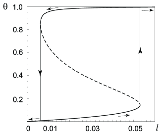
Figure 1: Adsorption isotherm for $g$ = 8.

The surface coverage $\theta$ increases with the concentration $\ell$ along the lower stable branch of the isotherm ending at the bifurcation concentration $\ell=\ell^{\textrm{b}}_{2}$ (here, $\ell^{\textrm{b}}_{1}\approx 0.0063$ and $\ell^{\textrm{b}}_{2}\approx 0.053$); furthermore, the increment of $\theta$ depends both on an increase in the gas concentration and on a variation in desorption properties of the adsorbent surface caused by the adsorbent deformation. The jump of $\theta$ to the upper stable branch of the isotherm at $\ell=\ell^{\textrm{b}}_{2}$ is caused exclusively by a change in desorption properties of the adsorbent. For convenience, transitions between stable branches of $\theta(\ell)$ are shown in figure 1 by light vertical straight lines with arrows indicating the direction of transition. Arrows under and above stable branches of $\theta(\ell)$ show the direction of variation in $\ell$. For $\ell>\ell^{\textrm{b}}_{2}\,$, the surface coverage $\theta$ varies with $\ell$ along the upper stable branch.

The transition of $\theta$ from the lower stable branch to the upper one at the bifurcation concentration $\ell^{\textrm{b}}_{2}$ is accompanied by a step increase in the activation energy for desorption, which hampers the desorption of adparticles from the surface. As a result, as the concentration $\ell$ decreases from a value greater than $\ell^{\textrm{b}}_{2}$, the reverse transition of $\theta$ from the upper stable branch to the lower one occurs at the lower bifurcation concentration $\ell^{\textrm{b}}_{1}<\ell^{\textrm{b}}_{2}$  at which the upper stable branch ends.

This behavior of the surface coverage $\theta$ versus the gas concentration $\ell$ corresponds to the well-known principle of perfect delay [34, 35].

The essentially different behavior of adsorption isotherms for $g\leqslant 4$ and $g>4$ depends on the varying shape of the function $V(\xi)$ (also called a potential) in these cases, namely [27]: $V(\xi)$ has a single well for $g\leqslant 4$ and for $g>4$, $\ell\notin[\ell^{\textrm{b}}_{1},\,\ell^{\textrm{b}}_{2}]$ and two wells with local minima at $\xi=\xi_{1}$ (the first well) and $\xi=\xi_{3}$ (the second well) separated by a maximum at $\xi=\xi_{2}\,$, where $\xi_{k}\,$, $k=1,2,3$, are the solutions of equation (21) for $g>4$, $\ell\in(\ell^{\textrm{b}}_{1},\,\ell^{\textrm{b}}_{2})$. In the last case, denote $V_{k}\equiv V(\xi_{k})$, where $k=1,2,3$, and, for a given $g$, the position of the absolute minimum of the potential $V(\xi)$ depends on the value of $\ell$. In the special case where system (11) has a two-fold stationary solution ($\xi^{\textrm{b}}_{1}$ for $\ell=\ell^{\textrm{b}}_{1}$ or $\xi^{\textrm{b}}_{2}$ for $\ell=\ell^{\textrm{b}}_{2}$), the potential $V(\xi)$ has a point of inflection at $\xi=\xi^{\textrm{b}}_{k}\,$, $k=1,2$, lying to the right (for $k=1$) or to the left (for $k=2$) of the bottom of the single well of $V(\xi)$.

We now dwell in detail on the bistable system with two energetically equivalent states ($V_{1}=V_{3}$). For any $g>4$, this important case occurs for the concentration $\ell_{\textrm{M}}$ defined as follows:

$$\ell_{\textrm{M}}=\exp\Bigl{(}-\frac{g}{2}\Bigr{)}\,.$$ (25)

Following [34, 35], the quantity $\ell_{\textrm{M}}$ for $g>4$ may be called a Maxwell concentration. It is directly verified that the potential $V(\xi)$ with $\ell=\ell_{\textrm{M}}$ denoted by $V^{\textrm{M}}(\xi)$,

$$V^{\textrm{M}}(\xi)=\widetilde{\xi}^{\,2}-\frac{1}{4}-\frac{1}{2\,q}\,\ln{\dfrac{\cosh{2\,q\,\widetilde{\xi}}}{\cosh{q}}}\,,\qquad\widetilde{\xi}=\xi-\frac{1}{2}\,,$$ (26)

is an even function about $\xi=1/2$. Hence, the function $V^{\textrm{M}}(\xi)$ (called a Maxwell potential) at $\xi=1/2$ has either the minimum (a single well for $q\leqslant 1$) or the maximum (two wells for $q>1$)

$$\widetilde{V}^{\textrm{M}}\equiv V^{\textrm{M}}\Bigl{(}\xi=\frac{1}{2}\Bigr{)}=\frac{\ln{\cosh{q}}}{2\,q}-\frac{1}{4}\,.$$ (27)

The double-well Maxwell potential $V^{\textrm{M}}(\xi)$ has equal minimal values denoted by $V^{\textrm{M}}_{\textrm{min}}$ at $\xi=\xi_{1}\equiv\xi^{\textrm{M}}_{-}$ and $\xi=\xi_{3}\equiv\xi^{\textrm{M}}_{+}\,$, where $\ \xi^{\textrm{M}}_{\pm}=(1\pm\eta/q)/2\,$ and $\eta$ is a positive solution of the equation

$$\frac{x}{q}=\tanh{x}\,.$$ (28)

This equation directly follows from (21) with $\ell=\ell_{\textrm{M}}$ or from the condition that the force $F(\xi)$ with $\ell=\ell_{\textrm{M}}$ denoted by $F^{\textrm{M}}(\xi)$,

$$F^{\textrm{M}}(\xi)=\frac{\varkappa}{2}\,\Bigl{(}\tanh 2\,q\,\widetilde{\xi}-2\,\widetilde{\xi}\Bigr{)}\,,\qquad\widetilde{\xi}=\xi-\frac{1}{2}\,,$$ (29)

is equal to zero. According to relations (26) and (27), the wells are separated by a barrier of the height $\,\Delta_{\textrm{M}}=\widetilde{V}^{\textrm{M}}-V^{\textrm{M}}_{\textrm{min}}\,$ relative to the bottoms of the wells,

$$\Delta_{\textrm{M}}=\frac{1}{2\,q}\,\Bigl{(}\ln{\cosh{\eta}}-\frac{\eta^{2}}{2\,q}\,\Bigr{)}\,.$$ (30)

In the case where the coupling parameter $g$ is close to the critical $g_{\textrm{c}}\,$, i.e., $q=1+\varepsilon,\ 0<\varepsilon\ll 1$, we obtain $\eta\approx\sqrt{3\,\varepsilon}$ and the very low barrier $\Delta_{\textrm{M}}\approx 3\,\varepsilon^{2}/8$ separating the closely spaced wells.

For $q\gg 1$, we get $\eta\approx q\,(1-2\,\ell_{\textrm{M}})$, which yields $\xi^{\textrm{M}}_{+}\approx 1-\ell_{\textrm{M}}\,$, $\xi^{\textrm{M}}_{-}\approx\ell_{\textrm{M}}$ and

$$V^{\textrm{M}}_{\textrm{min}}\approx-\ell_{\textrm{M}}^{\,2}\,,\qquad\widetilde{V}^{\textrm{M}}\approx\frac{1}{4}-\frac{\ln 2}{2\,q}\,.$$ (31)

In this case, the wells are far spaced and the barrier height $\Delta_{\textrm{M}}\approx\widetilde{V}^{\textrm{M}}$ tends to its maximum value equal to 1/4 as $g\rightarrow\infty$.

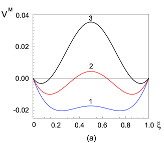
Figure 2: (Color online) The Maxwell potential $V^{\textrm{M}}(\xi)$ for: (a)  $g=$ 4.4 (1), 5 (2), 6 (3);  (b)  $g=$ 6 (1), 8 (2), 10 (3).

Figure 3: (Color online) The potential $V(\xi)$ for $g=8$ and the concentration $\ell=$ 0.01 (1), $\ell_{\textrm{M}}$ (2), 0.05 (3).

The curves in figure 2 show the behavior of the Maxwell potential $V^{\textrm{M}}(\xi)$ with the coupling parameter $g$, namely: the growth of the barrier between the wells and the motion of the wells from $\xi=1/2$.

The curves in figure 3 depicted for $g=8$ and $\ell\in(\ell^{\textrm{b}}_{1},\,\ell^{\textrm{b}}_{2})$, where $\ell^{\textrm{b}}_{1}\approx 0.0063$ and $\ell^{\textrm{b}}_{2}\approx 0.053$, clearly illustrate transformations of the double-well potential $V(\xi)$ with $\ell$. For $\ell\in(\ell^{\textrm{b}}_{1},\,\ell_{\textrm{M}})$, where $\ell_{\textrm{M}}\approx 0.0183$, the first well is deeper than the second one (curve 1). Thus, the system is stable in the first well and metastable in the second one. As $\ell\in(\ell^{\textrm{b}}_{1},\,\ell_{\textrm{M}})$ increases, the depths of both wells increase with $\ell$ but with different increments. For $\ell=\ell_{\textrm{M}}\,$, the double-well potential is symmetric about $\xi=1/2$ (curve 2). For $\ell\in(\ell_{\textrm{M}}\,,\,\ell^{\textrm{b}}_{2})$, the second well is deeper than the first (curve 3). Hence, the system is metastable in the first well and stable in the second one. However, according to the principle of perfect delay [34, 35], the oscillator, which was initially at rest in the first well, remains in this well with an increase in $\ell$ until the well disappears. For the transition of the oscillator from the first well into the deeper second well following the Maxwell principle [34, 35], it is necessary to take into account additional factors that enable the oscillator to overcome the barrier between the wells, e.g., fluctuations or the inertia effect (as in [36]). In the next section of the paper, to investigate transitions of the oscillator from one well into another, we take thermal fluctuations in the system into account.

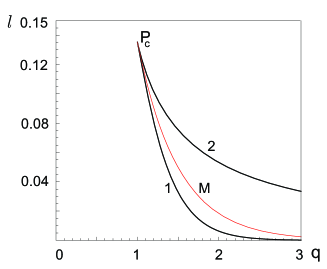
Figure 4: (Color online) Bifurcation curve (branches 1 and 2 of the curve correspond to the bifurcation concentrations $\ell^{\textrm{b}}_{1}$ and $\ell^{\textrm{b}}_{2}\,$, respectively) and the Maxwell set (curve M).

The bifurcation curve in the plane of control parameters $(q,\ell)$ in figure 4 divides the first quadrant of the plane into two parts. Branches 1 and 2 of the curve correspond to the bifurcation concentrations $\ell^{\textrm{b}}_{1}$ and $\ell^{\textrm{b}}_{2}\,$, respectively, defined by relations (22) and curve M is the Maxwell set of the values of the concentration $\ell_{\textrm{M}}$ for $q>1$ defined by (25). The domain outside the bifurcation curve is a domain of monostability of the system; for any point of this domain, system (11) has one asymptotically stable stationary solution. The open domain enclosed by the bifurcation curve is a domain of bistability of the system; for any point of this domain, system (11) has three stationary solutions (two asymptotically stable and one unstable). For any point of the bifurcation curve, except for the critical point $P_{\textrm{c}}\equiv(q_{\textrm{c}}\,,\,\ell_{\textrm{c}})$, where $q_{\textrm{c}}=1,\ \ell_{\textrm{c}}=\exp(-2)\approx 0.135$ is the critical concentration, which is the common point of the branches and the cusp of the second kind of the bifurcation curve, system (11) has two stationary solutions (one is asymptotically stable and the other one is two-fold). At the cusp, system (11) has one three-fold stationary solution. Curve M divides the domain of bistability into two subdomains: for any point lying between curves 1 and M, the system is stable in the first well and metastable in the second one; for any point lying between curves 2 and M, the system is stable in the second well and metastable in the first one. For any point of curve M, except for the point $P_{\textrm{c}}\,$, both wells have equal depths and, hence, two stable states of the system coexist and curve M is a curve of the coexistence of two stable states of the system. Taking into account thermal fluctuations in the system under study, we can conclude that the motion in the plane of control parameters $(q,\ell)$ along any line intersecting curve M is accompanied by the transition of the system from one well into another (deeper) well after the intersection of curve M. At the point of intersection of the line and curve M, the first-order phase transition occurs [35].

Given the explicit expression for the Maxwell concentration (25), we can easily plot the actual adsorption isotherms based on the Maxwell principle (and called Maxwell adsorption isotherms) on the basis of adsorption isotherms defined by relations (20), (21). To this end, we first note that, for $g>4$, each stable branch of an adsorption isotherm has a metastable part lying to the right (for the lower stable branch) or to the left (for the upper stable branch) of the point of the branch with abscissa $\ell=\ell_{\textrm{M}}\,$. A Maxwell adsorption isotherm consists of the corresponding adsorption isotherm defined by (20), (21) without the unstable branch and the metastable parts of the stable branches and the segment AB of the vertical straight line $\ell=\ell_{\textrm{M}}$ connecting the stable branches. Hence, a Maxwell adsorption isotherm is an adsorption isotherm of a system of adparticles having one stable state for any concentration $\ell$ except for the single concentration $\ell=\ell_{\textrm{M}}$ for which the system has two energy-equivalent states and which, following [17], may be called the phase transition concentration. Note that Maxwell adsorption isotherms thus constructed are similar to the well-known adsorption isotherms taking into account attractive lateral interactions between adparticles on a nondeformable adsorbent (see, e.g., [5, 7, 15, 16, 17]). Furthermore, the Maxwell concentration (25) agrees with the corresponding expression for the phase transition pressure for the classical Fowler-Guggenheim adsorption isotherms in the case of attractive lateral interactions of adparticles on a nondeformable adsorbent [17] if the maximum increment of the activation energy for desorption of adparticles $|V^{\textrm{a}}|$ caused by the adsorbent deformation in (12) is replaced by the modulus of the energy of attractive lateral interaction of two neighboring adparticles for $\theta=1$ multiplied by the coordination number of the lattice of adsorption sites.

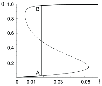
Figure 5: Adsorption isotherm (thin curve) and the Maxwell adsorption isotherm (thick curve) for $g$ = 8.

The adsorption isotherm and the Maxwell adsorption isotherm consisting of stable branches of the adsorption isotherm without metastable parts and the segment AB of the vertical straight line $\ell=\ell_{\textrm{M}}$ connecting the branches in figure 5 clearly illustrate the essential difference (the presence and absence of a hysteresis loop, respectively) in the behavior of the amount of adsorbed substance with $\ell$. The vertical part (the segment AB) of the Maxwell adsorption isotherm indicates the coexistence of two stable states of the system under study and corresponds to the first-order phase transition in the system. It is easy to see that the areas of the domains enclosed by the adsorption isotherm and the segment AB to the left and to the right of the segment AB are different. Nevertheless, the equality of these areas is proved. Furthermore, for any $g>4$ (and, hence, the well-known Maxwell rule of equal areas is true for the adsorption isotherms on a deformable adsorbent) if $\ln\ell$ is laid off along the abscissa axis instead of $\ell$ (see also the Maxwell rule of equal areas for the adsorption isotherms taking into account attractive lateral interactions between adparticles on a nondeformable adsorbent [16]). It is also worth noting that the ordinate of the point of intersection of the unstable branch of the adsorption isotherm and the vertical straight line $\ell=\ell_{\textrm{M}}$ is equal to $1/2$ for any value of $g$ due to the evenness of the Maxwell potential $V^{\textrm{M}}(\xi)$ about $\xi=1/2$.

According to the remark before figure 1, the thick curve in figure 5 also describes the actual (Maxwell) behavior of the adsorption-induced surface normal relaxation of a solid adsorbent with concentration $\ell$.

3 Probability density

To investigate transitions of the bistable system between its stable states with variation in the control parameters $\ell$ and $g$, we take into account thermal fluctuations in the system introducing a Langevin force $\mathcal{F}(t)$ in the right-hand side of the deterministic equation of motion of oscillator (17), [37, 38, 39] which yields the stochastic differential equation

$$\alpha\frac{\mathrm{d}x}{\mathrm{d}t}=F(x)+\mathcal{F}(t)\,.$$ (32)

The random force $\mathcal{F}(t)$ has the properties of a white noise:

$$\left\langle\mathcal{F}(t)\right\rangle=0\,,\qquad\left\langle\mathcal{F}(t)\,\mathcal{F}(t^{\prime})\right\rangle=2k_{\textrm{B}}T\alpha\,\delta(t-t^{\prime}),$$ (33)

where the angular brackets $\,\left\langle\ldots\right\rangle\,$ denote the averaging over an ensemble of realizations of the random force $\mathcal{F}(t)$, the quantity $2k_{\textrm{B}}T\alpha$ in the correlation function in (33) is the intensity of the Langevin force, and $\delta(x)$ is the Dirac $\delta$-function.

Following [38], we denote random variables by capital letters and their values by small letters (for example, $X(t)$ is a realization of the dynamical variable $x$ at the time $t$). Equation (32) can be reduced to the Fokker-Planck equation for the probability density $p(x,t)=\left\langle\delta\left(x-X(t)\right)\right\rangle$ of the coordinate of oscillator [37, 38, 39], which also describes the adsorption-induced surface normal relaxation of a solid adsorbent with regard for thermal fluctuations,

$$\alpha\,\frac{\partial p(x,t)}{\partial t}=\frac{\partial}{\partial x}\,\Biggl{[}\frac{\mathrm{d}U(x)}{\mathrm{d}x}\,p(x,t)+k_{\textrm{B}}T\,\frac{\partial p(x,t)}{\partial x}\Biggr{]}\,.$$ (34)

Given the quantity $p(x,t)$ as a solution of the Fokker-Planck equation (34), the probability density $p(\xi,t)$ of the random variable $\,\Xi\,$ is expressed in terms of $p(x,t)$ as follows:

$$p(\xi,t)=|x_{\textrm{max}}|\,p(x,t)\big{|}_{\,x=x_{\textrm{max}}\,\xi}\,.$$ (35)

By virtue of (13), the joint probability density $p(\xi,\theta;t)$ of the random variables and $\Xi$ and $\Theta$ has the form

$$p(\xi,\theta;t)=p(\xi,t)\,\delta\big{(}\theta-f(\xi)\big{)}\,,\qquad\theta\in[0,1],$$ (36)

where the $\delta$-function on the right-hand side of (36) is the conditional probability density $p(\theta|\,\xi;t)=\delta(\theta-f(\xi))$ with the sharp value for $\theta=f(\xi)$ and $f(\xi)$ is the deterministic function equal to the right-hand side of relation (13).

We first consider the stationary case. Under the natural boundary conditions, the stationary probability density $p(x)$ has the Boltzmann distribution [38, 39]

$$p(x)=\mathcal{N}\,\exp\left[-\frac{U(x)}{k_{\textrm{B}}T}\right],$$ (37)

where $\mathcal{N}$ is the normalization constant defined as follows:

$$\mathcal{N}^{-1}\,=\int\limits_{-\infty}^{\infty}\!\!\mathrm{d}x\,\exp\left[-\frac{U(x)}{k_{\textrm{B}}T}\right].$$ (38)

In view of (37), (16), and (19), we get

$$p(\xi)=\widetilde{\mathcal{N}}\,\exp\left[-\frac{g}{2}\,V(\xi)\right],$$ (39)

where

$$\widetilde{\mathcal{N}}=|x_{\textrm{max}}|\,\mathcal{N}=\sqrt{\frac{g}{2\pi}}\,\frac{1+\ell}{1+\lambda}\,,\qquad\lambda=\frac{\ell}{\ell_{\textrm{M}}}\,.$$ (40)

According to (39), the functions $p(\xi)$ and $V(\xi)$ have extrema at the same points, moreover, if $V(\xi)$ has a minimum (maximum) at some point, then $p(\xi)$ has a maximum (minimum) at this point [38, 39]. Hence, the stationary probability density $p(\xi)$ is single-modal for $g\leqslant 4$ and for $g>4$, $\ell\notin[\ell^{\textrm{b}}_{1}\,,\,\ell^{\textrm{b}}_{2}]$ and bimodal for $g>4$, $\ell\in(\ell^{\textrm{b}}_{1}\,,\,\ell^{\textrm{b}}_{2})$.

By using the explicit expression (16) for $V(\xi)$, we obtain

$$p(\xi)=\sqrt{\frac{g}{2\pi}}\,\exp{\left(-\frac{g\,\xi^{2}}{2}\right)}\,\frac{1+\ell\,\exp{(g\,\xi)}}{1+\lambda}\,,\qquad p(x)=\frac{1+\ell\,\exp{(b\,x)}}{1+\lambda}\,p_{0}(x),$$ (41)

where

$$p_{0}(x)=\frac{1}{\sqrt{2\,\pi}\,\sigma_{0}}\,\exp{\left(-\frac{x^{2}}{2\,\sigma_{0}^{2}}\right)}$$ (42)

is the Gaussian distribution of the probability density for a linear oscillator with zero mean ($\left\langle X\right\rangle\,=0$) and the variance $\sigma_{0}^{2}=k_{\textrm{B}}T/\varkappa$.

We first consider the single-modal stationary probability density $p(x)$. In this case, the random variable $X$ has the nonzero mean

$$\left\langle X\right\rangle\,=\,\frac{\lambda}{1+\lambda}\>x_{\textrm{max}}\,,$$ (43)

which yields $\,\mathop{\rm sign}\nolimits\left\langle X\right\rangle\,=\mathop{\rm sign}\nolimits\,\chi$ and, hence, the maximum of the probability density $p(x)$ shifts in the direction of the action of the adsorption-induced force; the variance $\sigma^{2}\equiv\,\left\langle(X\,-\langle X\right\rangle)^{2}\rangle$,

$$\sigma^{2}=\left[1+g\,\frac{\lambda}{(1+\lambda)^{2}}\right]\,\sigma_{0}^{2}\,,$$ (44)

which is greater than $\sigma_{0}^{2}$ for any values of the concentration and the coupling parameter and, for a fixed value of $g$, reaches its maximum value equal to $(1+q)\,\sigma_{0}^{2}\,$ for $\lambda=1$; the asymmetry ratio $S=\langle(X\,-\left\langle X\right\rangle)^{3}\rangle/\sigma^{3}$,

$$S=g^{3/2}\,\frac{\lambda\,(1-\lambda^{2})(1+\lambda)^{2}}{[(1+\lambda)^{2}+g\,\lambda]^{3}}\,\mathop{\rm sign}\nolimits\,\chi,$$ (45)

and, hence, $\,\mathop{\rm sign}\nolimits\,S=\mathop{\rm sign}\nolimits\,\big{(}(\ell_{\textrm{M}}-\ell)\,\chi\big{)}$, which implies the change in the sign of the asymmetry ratio in crossing the concentration $\ell_{\textrm{M}}\,$; and the excess (flatness) $E=\langle(X\,-\left\langle X\right\rangle)^{4}\rangle/\sigma^{4}-3$,

$$E=g^{2}\,\frac{\lambda\,(1+\lambda^{2}-4\,\lambda)}{[(1+\lambda)^{2}+g\,\lambda]^{2}}\,.$$ (46)

According to (46), the probability density $p(x)$ is flat-topped ($E<0)$ for $\ell\in(\ell_{-}\,,\,\ell_{+})$, where $\ell_{\pm}=(2\pm\sqrt{3})\,\ell_{\textrm{M}}\,$, or peaked ($E>0$) for $\ell\notin[\ell_{-}\,,\,\ell_{+}]$ relative to the Gaussian distribution with mean (43) and variance (44). For $\ell=\ell_{-}$ and $\ell=\ell_{+}\,$, $E=0$ as for this Gaussian distribution.

In the Maxwell case ($\ell=\ell_{\textrm{M}}$), the probability density $p(x)$ in (41) denoted by $p_{\textrm{M}}(x)$ is simplified to the form

$$p_{\textrm{M}}(x)=\frac{\ell_{\textrm{M}}^{1/4}}{\sqrt{2\,\pi}\,\sigma_{0}}\,\exp{\left(-\frac{\tilde{x}^{2}}{2\,\sigma_{0}^{2}}\,\right)}\,\cosh{\left(\frac{b\,\tilde{x}}{2}\right)}\,,\qquad\tilde{x}=x-\frac{x_{\textrm{max}}}{2}\,,$$ (47)

which is an even function about $x=x_{\textrm{max}}/2$.

In the single-modal case ($g\leqslant 4$), we have $\left\langle X\right\rangle=x_{\textrm{max}}/2$, $\sigma^{2}=(1+q)\sigma_{0}^{2}$, $S=0$, and $E=-2q^{2}/(1+q)^{2}<0$. Hence, $p_{\textrm{M}}(x)$ is a flat-topped distribution symmetric about its maximum value equal to   $\ell_{\textrm{M}}^{1/4}/(\sqrt{2\,\pi}\,\sigma_{0})$  at $x=x_{\textrm{max}}/2$.

We now investigate the transition of the bistable system from one stable state to another due to thermal fluctuations. This transition occurs for the double-well potential $V(\xi)$ studied above: the left-hand and right-hand wells with minimal values $V_{\textrm{L}}\equiv V_{1}$ and $V_{\textrm{R}}\equiv V_{3}\,$, respectively, at $\xi=\xi_{1}\equiv\xi_{\textrm{L}}\,$ and $\xi=\xi_{3}\equiv\xi_{\textrm{R}}$ are separated by the barrier with maximum value $V_{\textrm{B}}\equiv V_{2}$ at $\xi=\xi_{2}\equiv\xi_{\textrm{B}}\,$. By using the Gardiner representation [38] of the Kramers method [40], the following system of equations is derived from the Fokker-Planck equation (34):

$$\left\{\begin{array}[]{l}\dfrac{\mathrm{d}P_{\textrm{L}}(t)}{\mathrm{d}t}=-k_{\textrm{L}}\,P_{\textrm{L}}(t)+k_{\textrm{R}}\,P_{\textrm{R}}(t),\vspace{3mm}\\ \dfrac{\mathrm{d}P_{\textrm{R}}(t)}{\mathrm{d}t}=-k_{\textrm{R}}\,P_{\textrm{R}}(t)+k_{\textrm{L}}\,P_{\textrm{L}}(t).\end{array}\right.$$ (50)

This system describes the evolution of the probabilities of the presence of an oscillator to the left (in the left-hand well), $P_{\textrm{L}}(t)$, and to the right (in the right-hand well), $P_{\textrm{R}}(t)$, of the point $\xi_{\textrm{B}}$ at time $t$ under the assumption that the relaxation times of the oscillator in the wells are much less than the mean transition times between the wells

$$P_{\textrm{L}}(t)=\int\limits_{-\infty}^{\xi_{\textrm{B}}}\!\!\mathrm{d}\xi\,p(\xi,t),\qquad P_{\textrm{R}}(t)=\int\limits_{\xi_{\textrm{B}}}^{\infty}\!\!\mathrm{d}\xi\,p(\xi,t),\qquad P_{\textrm{L}}(t)+P_{\textrm{R}}(t)=1.$$ (51)

Here,

$$k_{i}=\frac{1}{g\mu\,P_{i}\,\tau_{\text{r}}}\,,\qquad i=\textrm{L,\,R},$$ (52)

is the coefficient of the escape rate of an oscillator from the $i$th well ($i=\textrm{L,\,R}$) derived under the assumption of a vanishing probability of the presence of the oscillator in the well outside a small neighborhood of $\xi_{i}\,$, $i=\textrm{L,\,R}$, and $P_{i}$ is the probability of the presence of the oscillator in the $i$th well ($i=\textrm{L,\,R}$) in the stationary case, i.e.,

$$P_{\textrm{L}}=\int\limits_{-\infty}^{\xi_{\textrm{B}}}\!\!\mathrm{d}\xi\,p(\xi)\,,\qquad P_{\textrm{R}}=\int\limits_{\xi_{\textrm{B}}}^{\infty}\!\!\mathrm{d}\xi\,p(\xi)\,$$ (53)

and

$$\mu=\int\limits_{\xi_{\textrm{L}}}^{\xi_{\textrm{R}}}\!\!\frac{\mathrm{d}\xi}{p(\xi)}\,.$$ (54)

The solution of system (50) has the form

$$P_{i}(t)=P_{i}^{0}\,\exp{\left(-\frac{t}{T_{+}}\right)}+P_{i}\,\left[1-\exp{\left(-\frac{t}{T_{+}}\right)}\right]\,,\qquad i=\textrm{L,\,R},$$ (55)

where $P_{i}^{0}$ is the initial value of the probability $P_{i}(t),\,i=\textrm{L,\,R}$, for $t=0$, $k_{+}=k_{\textrm{L}}+k_{\textrm{R}}\,$, and

$$T_{+}=1/k_{+}=g\mu\,P_{\textrm{L}}\,P_{\textrm{R}}\,\tau_{\text{r}}$$ (56)

is the relaxation time of the quantity $P_{i}(t)$, $i=\textrm{L,\,R}$.

According to (50), the mean transition time from one stable state at $\xi=\xi_{i}$ to another at $\xi=\xi_{j}\,$, where $i,j=\textrm{L,\,R}$, $i\neq j$, is defined as $T_{i\,\rightarrow\,j}=1/k_{i}$ and, with regard for (52), has the form

$$T_{i\,\rightarrow\,j}=g\mu\,P_{i}\,\tau_{\text{r}}\,,\qquad i,j=\textrm{L,\,R},\qquad i\neq j,$$ (57)

which yields the well-known relationship [41] between the probabilities $P_{i}$ and the mean transition times $T_{i\rightarrow j}$:

$$\frac{P_{\textrm{L}}}{P_{\textrm{R}}}=\frac{T_{\textrm{L}\,\rightarrow\,\textrm{R}}}{T_{\textrm{R}\,\rightarrow\,\textrm{L}}}\,.$$ (58)

In the parabolic approximation [38, 41] of the potential $U(\xi)$ (16) in the neighborhoods of its extrema, the mean transition times $T_{i\,\rightarrow\,j}$ are estimated as follows:

$$T_{i\,\rightarrow\,j}\approx\tau_{\text{r}}\,\frac{2\pi}{\sqrt{L(\xi_{i},g)\,|L(\xi_{2},g)|}}\,\exp{\Bigl{(}\frac{g}{2}\,\Delta_{\,\textrm{B},\,i}\Bigr{)}},\qquad i,j=\textrm{L,\,R},\qquad i\neq j,$$ (59)

where

$$\Delta_{\,i,j}=V_{i}-V_{j}=(\xi_{i}-\xi_{j})\,(\xi_{i}+\xi_{j}-2)\,+\frac{2}{g}\,\ln{\frac{\xi_{i}}{\xi_{j}}}\,,\qquad i,j=\textrm{L,\,R,\,B},$$ (60)

$$L(\xi,g)=1+g\xi\,(\xi-1)$$ (61)

is an even function about $\xi=1/2$ such that, for $g>4$, $1>L(\xi_{i}\,,g)>0$, $i=\textrm{L,\,R},$ and $L(\xi_{\text{B}}\,,g)<0$.

In this approximation, the quantity

$$\tau_{i}=\frac{\tau_{\text{r}}}{L(\xi_{i},g)}\,,\qquad i=\textrm{L,\,R},$$ (62)

has the sense of the mean relaxation time of an overdamped oscillator in the left-hand ($i=\textrm{L}$) or in the right-hand ($i=\textrm{R}$) parabolic potential well centered at $\xi=\xi_{i}$ and derived from (16). Hence, in this approximation, the restoring force constant $\varkappa$ is simply replaced by $\varkappa_{i}$ = $\varkappa\,L(\xi_{i}\,,g)$, $i=\textrm{L,\,R}$, that already depends on $\ell$ and $g$, which yields $\tau_{i}>\tau_{\text{r}}\,$, $i=\textrm{L,\,R}$.

If the concentration $\ell\in(\ell^{\textrm{b}}_{1}\,,\,\ell^{\textrm{b}}_{2})$ approaches the end point of the interval of bistability ($\ell^{\textrm{b}}_{1}$ or $\ell^{\textrm{b}}_{2}$), then $L(\xi_{\textrm{R}}\,,g)$ or $L(\xi_{\textrm{L}}\,,g)$, respectively, tends to zero. According to (62), this is accompanied by an essential increase in the relaxation time $\tau_{\textrm{R}}$ (in the first case) or $\tau_{\textrm{L}}$ (in the second case) due to the flattening of the corresponding well. This indicates that the parabolic approximation is false in small neighborhoods of the bifurcation concentrations $\ell^{\textrm{b}}_{1}$ and $\ell^{\textrm{b}}_{2}$ because the very shallow right-hand (in the first case) and left-hand (in the second case) wells are almost flat-bottomed.

Formally introducing the quantity

$$\tau_{\textrm{B}}=\frac{\tau_{\text{r}}}{|\textrm{L}(\xi_{\textrm{B}}\,,g)|}\,,$$ (63)

which can be regarded as the mean relaxation time of an overdamped oscillator in the parabolic potential well centered at $\xi=\xi_{\textrm{B}}$ and derived from (16) with $|L(\xi_{\textrm{B}}\,,g)|$ instead of $L(\xi_{\textrm{B}}\,,g)$, we can express the mean transition times $T_{i\,\rightarrow\,j}$ (59) in terms of the relaxation times of an overdamped oscillator in the corresponding parabolic potential wells as follows:

$$T_{i\,\rightarrow\,j}\approx 2\pi\,\sqrt{\tau_{i}\,\tau_{\textrm{B}}}\,\exp{\Bigl{(}\frac{g}{2}\,\Delta_{\,\textrm{B}\,,\,i}\Bigr{)}}\,,\qquad i,j=\textrm{L,\,R},\qquad i\neq j,$$ (64)

which agrees with the classical Kramers formula in the overdamped case [40].

The assumption of two time scales (the short time scale for the relaxation of the oscillator in the well where it was at the initial time and at the long-time scale for the transition of the oscillator from one stable state to another across the unstable state) used in the derivation of system (50) imposes the following condition on the Arrhenius factor:

$$\exp{\Bigl{(}\frac{g}{2}\,\Delta_{\,\textrm{B},\,i}\Bigr{)}}\gg\frac{1}{2\pi}\,\sqrt{\frac{\tau_{i}}{\tau_{\textrm{B}}}}\,,\qquad i=\textrm{L,\,R}\,.$$ (65)

Substituting (60) in (59) and (64), we express the ratio of the mean transition times between the wells in terms of the coordinates of their minima $\xi_{\textrm{L}}\,$ and $\xi_{\textrm{R}}\,$ as follows:

$$\frac{T_{\textrm{L}\,\rightarrow\,\textrm{R}}}{T_{\textrm{R}\,\rightarrow\,\textrm{L}}}=\sqrt{\frac{\tau_{\textrm{L}}}{\tau_{\textrm{R}}}}\,\exp{\Bigl{(}\frac{g}{2}\,\Delta_{\,\textrm{R,\,L}}\Bigr{)}}=\sqrt{\frac{\tau_{\textrm{L}}}{\tau_{\textrm{R}}}}\,\frac{\xi_{\textrm{R}}}{\xi_{\textrm{L}}}\,\exp{\Bigl{[}\frac{g}{2}\,(\xi_{\textrm{R}}-\xi_{\textrm{L}})\,(\xi_{\textrm{R}}+\xi_{\textrm{L}}-2)\Bigr{]}}\,.$$ (66)

For the Maxwell potential (26), we get $\xi_{\textrm{B}}=1/2$, the quantity $L(\xi_{\textrm{B}}\,,g)=1-q$   is independent of the concentration and, hence, $\tau_{\textrm{B}}=\tau_{\text{r}}/(q-1)$,

$$L(\xi_{\textrm{L}}\,,g)=L(\xi_{\textrm{R}}\,,g)\equiv L_{\textrm{M}}(g)=1-q\left(1-\frac{\eta^{2}}{q^{2}}\right)\,,\qquad\tau_{\textrm{L}}=\tau_{\textrm{R}}\equiv\tau_{\textrm{M}}=\frac{\tau_{\text{r}}}{\textrm{L}_{\textrm{M}}(g)}\,,$$ (67)

where, as above, $\eta$ is a positive solution of equation (28), equal mean transition times between the wells, $T_{\textrm{L}\,\rightarrow\,\textrm{R}}=T_{\textrm{R}\,\rightarrow\,\textrm{L}}\equiv T_{\textrm{M}}$ and, with regard for (60), (64), and (67),

$$T_{\textrm{M}}\approx 2\pi\,\sqrt{\tau_{\textrm{M}}\,\tau_{\textrm{B}}}\,\cosh{\eta}\,\exp{\left(-\frac{\eta^{2}}{2q}\right)}\,.$$ (68)

It is worth noting that expression (68) cannot be used if $q$ is close to 1 because, in this case, the assumptions of derivation of $T_{\textrm{M}}$ are violated.

For large values of the coupling parameter, $q\gg 1$, the quantity $\eta\approx q\,(1-2\,\ell_{\textrm{M}})$, which yields $\tau_{\textrm{M}}\approx\tau_{\text{r}}\,$, $\tau_{\textrm{B}}\approx\tau_{\text{r}}/q$,

$$T_{\textrm{M}}\approx\tau_{\text{r}}\,\frac{\pi}{\sqrt{q}}\,\exp{\Bigl{(}\frac{q}{2}\Bigr{)}}\,.$$ (69)

In terms of the potential $U(x)$, we have $U(x=x_{\textrm{max}}/2)/k_{\textrm{B}}T\approx q/2$  for $q\gg 1$, which leads to the exponential growth of the mean transition time (69) with an increase in the coupling parameter $g$.

Relations for the mean transition times derived in the general case are given in Appendix.

4 Conclusions

In the present paper, we have investigated the problem of adsorption of a gas on the flat surface of a solid deformable nonporous adsorbent with regard for thermal fluctuations and analyzed the effect of thermal fluctuations on the normal displacement of the adsorbent surface and, hence, on the amount of adsorbed substance. We have derived explicit expressions for the mean transitions times between stable states of the bimodal system and investigated the dependence of these times on the values of the coupling parameter and the gas concentration.

According to the established results, the behavior of the system under study is most interesting for the case where the system is bistable. For the bistability of a system, the coupling parameter must exceed the threshold value. Thus, first of all, the value of the coupling parameter for the investigated adsorbent–adsorbate system should be calculated. However, this requires an additional information because the coupling parameter is expressed in terms of the phenomenological constant adsorption-induced force $\chi$. Nevertheless, this unknown force (and, hence, the coupling parameter) can be expressed in terms of the maximum change in the first interplanar spacing $x_{\textrm{max}}$ in the case of the total monolayer coverage of the adsorbent surface by adparticles:

$$\chi=\varkappa\,x_{\textrm{max}}\,,\qquad g=\varkappa\,x^{2}_{\textrm{max}}/k_{\textrm{B}}T.$$ (70)

Having the experimental value of $x_{\textrm{max}}$ for such an adsorbent–adsorbate system measured with proper accuracy, the value of the coupling parameter is easily calculated by using the second relation in (70). Given a base of experimental data (lacking at present) for $x_{\textrm{max}}$ for various adsorbent–adsorbate systems, one can select systems for which the established effects of bistability of the system caused by the adsorption-induced deformation of the adsorbent are possible.

Since the coupling parameter is proportion to $x^{2}_{\textrm{max}}$ (70), experiments with solid nonporous adsorbents with flat surface should be performed for materials with a considerable value of the adsorption-induced normal displacement of the surface.

Note that the results established in the present paper have been obtained for the model imposing the restrictions on the values of characteristic times (the average time between collisions of gas particles with an adsorption site, the average residence time of an adparticle on the surface, and the relaxation time of a bound adsorption site) and the friction coefficient.

Since the proposed model of adsorption on a deformable solid adsorbent does not take into account lateral interactions between adparticles, it is of interest to generalize this model to the case taking into account the joint action of both factors (adsorption-induced deformation of the adsorbent and lateral interactions between adparticles).

Appendix

The mean transition times $T_{i\,\rightarrow\,j}$ (64) derived above in the parabolic approximation can also be determined for the general case. By using expression (16) for $V(\xi)$ and relations (39)–(41), (52)–(54), and (57), we obtain the following relations for stationary probabilities:

$$P_{\textrm{R}}=\frac{1}{2\,(1+\lambda)}\,\Bigl{[}\mathop{\rm erfc}\nolimits\left(\sqrt{2\,q}\,\xi_{\textrm{B}}\right)+\lambda\,\mathop{\rm erfc}\nolimits\left(\sqrt{2\,q}\,(\xi_{\textrm{B}}-1)\right)\Bigr{]}\,,\qquad P_{\textrm{L}}=1-P_{\textrm{R}}\,,$$ (A.1)

and the mean transition times

$$T_{i\,\rightarrow\,j} =\tau_{\text{r}}\,P_{i}\,2(1+\lambda)\,\sqrt{\pi}\sum_{n=0}^{\infty}\frac{(-1)^{n}}{\ell^{n+1}}\,\exp{\left\{-2q\,\xi_{\textrm{L}}\,[2(n+1)-\xi_{\textrm{L}}]\right\}}\Bigl{\{}F\left(\sqrt{2\,q}\,(n+1-\xi_{\textrm{L}})\right)$$

$$\quad-\exp{\left\{2q\,(\xi_{\textrm{L}}-\xi_{\textrm{R}})\,[2(n+1)-\xi_{\textrm{L}}-\xi_{\textrm{R}}]\right\}}\,F\left(\sqrt{2\,q}\,(n+1-\xi_{\textrm{R}})\right)\Bigr{\}}\,,\qquad i,j=\textrm{L,\,R},\qquad i\neq j\,.$$ (A.2)

Here,

$$\mathop{\rm erfc}\nolimits(z)=\frac{2}{\sqrt{\pi}}\,\int\limits_{z}^{\infty}\!\!\mathrm{d}t\,\exp{\left(-t^{2}\right)}$$

is the complementary error function [42], the special function [43]

$$F(z)=\exp{(-z^{2})}\,\int\limits_{0}^{z}\!\!\mathrm{d}t\,\exp{\left(t^{2}\right)},$$

which is expressed in terms of the error function of imaginary argument, is bounded for all real $z$, has the maximum value $\approx 0.541$ for $z\approx 0.924$, the known power expansion for $|z|<\infty$, and the asymptotic formula $F(z)\approx 1/(2z)$ as $z\rightarrow\infty$.

In the Maxwell case ($\ell=\ell_{\textrm{M}}$), relations (A.1) yield equal values of the probabilities of the presence of the oscillator in both wells: $P_{\textrm{L}}=P_{\textrm{R}}=1/2$, which is quite natural for the symmetric Maxwell double-well potential (26). Relations (A.2) are reduced to the Maxwell mean transition time

$$T_{\textrm{M}}=\tau_{\text{r}}\,4\sqrt{\pi}\,\exp{\Bigl{(}\frac{q}{2}\Bigr{)}}\,\sum_{n=0}^{\infty}(-1)^{n}\,S_{n}(q),$$ (A.3)

where

$$S_{n}(q)=F(\beta_{n})-\exp{[-\gamma\,(2\,\beta_{n}-\gamma)]}\,F(\beta_{n}-\gamma)\,,\qquad\beta_{n}=\sqrt{\frac{q}{2}}\,(2n+1),\qquad\gamma=\frac{\eta}{\sqrt{2\,q}}\,,$$ (A.4)

$\eta$ is a positive solution of equation (28).

For $q\gg 1$, relation (A.3) is simplified to the form

$$T_{\textrm{M}}\approx\tau_{\text{r}}\,\frac{\pi^{3/2}}{\sqrt{2\,q}}\,\exp{\Bigl{(}\frac{q}{2}\Bigr{)}}\,.$$ (A.5)

Comparing (A.5) and (69) derived for the general case and in the parabolic approximation, respectively, we see that, for large values of $q,$ the mean transition times differ only by the factor $\sqrt{\pi/2}$ .

Ukrainian 0

Iндукована адсорбцiєю нормальна релаксацiя поверхнi твердого адсорбенту О.С. Усенко

             
Iнститут теоретичної фiзики iм. М.М. Боголюбова НАН України,
вул. Метрологiчна 14 б, 03680 Київ, Україна

References

- [1] Morrison S.R., The Chemical Physics of Surfaces, Plenum, New York, 1977.
- [2] Naumovets A.G., Ukr. J. Phys., 1978, 23, 1585 (in Russian).
- [3] Jaycock M.J., Parfitt G.D., Chemistry of Interfaces, Wiley, New York, 1981.
- [4] Kiselev V.F., Krylov O.V., Adsorption Processes on Semiconductor and Dielectric Surfaces, Springer, Berlin, 1985.
- [5] Zhdanov V.D., Elementary Physicochemical Processes on Solid Surfaces, Plenum, New York, 1991.
- [6] Lyuksyutov I.F., Naumovets A.G., Pokrovsky V.L., Two-Dimensional Crystals, Academic Press, Boston, 1992.
- [7] Adamson A.W., Cast A.P., Physical Chemistry of Surfaces, Wiley, New York, 1997.
- [8] Naumovets A.G., In: Progressive Materials and Technologies Vol. 2, Pokhodnya I.K., Kostornov A.H., Koval’ Yu.M., Lobanov L.M., Naidek V.L., et al. (Eds.), Akademperiodyka, Kyiv, 2003, 319–350 (in Russian).
- [9] Barret P., Cinétique Hétérogène, Guathier-Villars, Paris, 1973.
- [10] Roginskii S.Z., Heterogeneous Catalysis. Some Problems of the Theory, Nauka, Moscow, 1979 (in Russian).
- [11] Rozovskii A.Ya., Heterogeneous Chemical Reactions. Kinetics and Macrokinetics, Nauka, Moscow, 1980 (in Russian).
- [12] Boreskov G.K., Heterogeneous Catalysis, Nauka, Moscow, 1986 (in Russian).
- [13] Krylov O.V., Shub B.R., Nonequilibrium Processes in Catalysis, CRC Press, Boca Raton, 1994.
- [14] Ruthven D.M., Principles of Adsorption and Adsorption Processes, Wiley, Chichester, 1984.
- [15] Tovbin Yu.L., Theory of Physical Chemistry Processes at a Gas–Solid Interface, CRC Press, Boca Raton, 1991.
- [16] Rudzinski W., Everett D.H., Adsorption of Gases on Heterogeneous Surfaces, Academic Press, London, 1992.
- [17] Do D.D., Adsorption Analysis: Equilibria and Kinetics, Imperial College Press, London, 1998.
- [18] Keller J., Staudt R., Gas Adsorption Equilibria: Experimental Methods and Adsorption Isotherms, Springer, Berlin, 2005.
- [19] Imbihl R., Ertl G., Chem. Rev., 1995, 95, 697; doi:10.1021/cr00035a012.
- [20] Imbihl R., Catal. Today, 2005, 105, 206; doi:10.1016/j.cattod.2005.02.045.
- [21] Imbihl R., Surf. Sci., 2009, 603, 1671; doi:10.1016/j.susc.2008.11.042.
- [22] Ertl G., Reactions at Solid Surfaces, Wiley, Hoboken, 2009.
- [23] Tvardovskiy A.V., Sorbent Deformation, Elsevier, Amsterdam, 2007.
- [24] Ravikovitch P.I., Neimark A.V., Langmuir, 2006, 22, 10864; doi:10.1021/la061092u.
- [25] Gor G.Yu., Neimark A.V., Langmuir, 2010, 26, 13021; doi:10.1021/la1019247.
- [26] Gor G.Yu., Neimark A.V., Langmuir, 2011, 27, 6926; doi:10.1021/la201271p.
- [27] Usenko A.S., Phys. Scr., 2012, 85, 015601; doi:10.1088/0031-8949/85/01/015601.
- [28] Zeldovich Ya.B., Acta Physicochim. U.R.S.S., 1938, 8, 527.
- [29] Ala-Nissila T., Ferrando R., Ying S.G., Adv. Phys., 2002, 51, 949; doi:10.1080/00018730110107902.
- [30] Naumovets A.G., Surf. Sci., 1994, 299-300, 706; doi:10.1016/0039-6028(94)90691-2.
- [31] Andronov A.A., Vitt A.A., Khaikin S.É., Theory of Oscillators, Pergamon, New York, 1966.
- [32] Haken H., Synergetics, Springer, Berlin, 1978.
-
[33]
Christophorov L.N., Holzwarth A.R., Kharkyanen V.N.,
van Mourik F., Chem. Phys., 2000, 256, 45;
doi:10.1016/S0301-0104(00)00089-6. - [34] Poston T., Stewart I., Catastrophe Theory and Its Applications, Pitman, London, 1978.
- [35] Gilmore R., Catastrophe Theory for Scientists and Engineers, Wiley, New York, 1981.
- [36] Usenko A.S., Preprint arXiv:cond-mat.matrl-sci/0907.5569v2, 2009.
- [37] Rytov S.M., Introduction to Statistical Radiophysics. Part 1. Random Processes, Springer, Berlin, 1985.
- [38] Gardinder C.W., Handbook of Stochastic Methods for Physics, Chemistry and the Natural Sciences, Springer, Berlin, 1985.
- [39] Risken H., The Fokker-Planck Equation. Methods of Solution and Applications, Springer, Berlin, 1989.
- [40] Kramers H.A., Physica, 1940, 7, 282; doi:10.1016/S0031-8914(40)90098-2.
- [41] Van Kampen N.G., Stochastic Processes in Physics and Chemistry, North-Holland, Amsterdam, 1984.
- [42] Handbook of Mathematical Functions with Formulas, Graphs and Mathematical Tables. National Bureau of Standards Applied Mathematics Series Vol. 55, Abramowitz M., Stegun I.A. (Eds.), U.S. Government Printing Office, Washington, D.C., 1964.
- [43] Lebedev N.N., Special Functions and Their Applications, Prentice-Hall, Englewood Cliffs, 1965.
Ukrainian \adddialect\l@ukrainian0 \l@ukrainian