Neutrino mixing matrix and masses from a generalized Friedberg-Lee model

Abstract

The overall characteristics of the solar and atmospheric neutrino oscillation are approximately consistent with a tribimaximal form of the mixing matrix $U$ of the lepton sector. Exact tribimaximal mixing leads to $\theta_{13}=0$. However, recent results from Daya Bay and RENO experiments have established a nonzero value for $\theta_{13}$. Keeping the leading behavior of $U$ as tribimaximal, we use a generalized Fridberg-Lee neutrino mass model along with a complementary ansatz to incorporate a nonzero $\theta_{13}$ along with CP violation. We generalize this model in two stages: In the first stage we assume $\mu-\tau$ symmetry and add imaginary components which leads to nonzero phases. In the second stage we add a perturbation with real components which breaks the $\mu-\tau$ symmetry and this leads to a nonzero value for $\theta_{13}$. The combination of these two generalizations leads to CP violation. Using only two of the experimental data, we can fix all of the parameters of our model and predict not only values for the other experimental data, which agree well with the available data, but also the masses of neutrinos and the CP violating phases and parameters. These predictions include the following: $\langle m_{\nu_{e}}\rangle\approx(0.033-0.037)~{}eV$, $\langle m_{\nu_{\mu}}\rangle\approx(0.043-0.048)~{}eV$, $\langle m_{\nu_{\tau}}\rangle\approx(0.046-0.051)~{}eV$, and $59.21^{\circ}\lesssim\delta\lesssim 59.34^{\circ}$

1 Introduction

The remarkable experimental achievements resulting in experimental data for solar, atmospheric, accelerator and reactor neutrinos [1] give us information about neutrino masses and mixing which can be summarized as follows in Table 1 [2, 3]:

Parameter	The experimental data	The best fit ($\pm 1\sigma$)
$\Delta m_{21}^{2}[10^{-5}eV^{2}]$	$7.12-8.20$	$7.43-7.81$
$|\Delta m_{31}^{2}|[10^{-3}eV^{2}]$	$2.13-2.74$	$2.46-2.61$
	$2.21-2.64$	$2.37-2.50$
$\sin^{2}\theta_{12}$	$0.27-0.37$	$0.303-0.336$
$\sin^{2}\theta_{13}$	$0.017-0.033$	$0.0218-0.0275$
		$0.0223-0.0276$
$\sin^{2}\theta_{23}$	$0.36-0.68$	$0.400-0.461~{}\text{and}~{}0.573-0.635$
	$0.37-0.67$	$0.569-0.626$
$\delta$	$0-2\pi$	$0-2\pi$

Table 1: The experimental data for the neutrinos’ mixing parameters. In the last column, when multiple sets of allowed ranges are stated, the upper row corresponds to normal hierarchy and the lower raw to inverted hierarchy.

The lepton mixing matrix in the standard parametrization is given by [4, 5],

$$U_{PMNS}=\left(\begin{array}[]{ccc}c_{12}c_{13}&s_{12}c_{13}&s_{13}e^{-i\delta}\\ -s_{12}c_{23}-c_{12}s_{23}s_{13}e^{i\delta}&c_{12}c_{23}-s_{12}s_{23}s_{13}e^{i\delta}&s_{23}c_{13}\\ s_{12}s_{23}-c_{12}c_{23}s_{13}e^{i\delta}&-c_{12}s_{23}-s_{12}c_{23}s_{13}e^{i\delta}&c_{23}c_{13}\end{array}\right)\left(\begin{array}[]{ccc}1&0&0\\ 0&e^{i\rho}&0\\ 0&0&e^{i\sigma}\end{array}\right),$$ (1)

where $c_{ij}\equiv\cos\theta_{ij}\text{ and }s_{ij}\equiv\sin\theta_{ij}$ (for $i,j=(1,2),(1,3)\text{ and }(2,3)$). The phase $\delta$ is called the Dirac phase, analogous to the CKM phase, and the phases $\rho$ and $\sigma$ are called the Majorana phases and are relevant for Majorana neutrinos. However, we should mention that recently the advantages of the original symmetrical form of the parameterizations of the lepton mixing matrix has been discussed [5].

A relatively successful phenomenological Ansats for the neutrino mixing matrix was proposed by Harrison, Perkins and Scott in 2002 [6], and is known as the tribimaximal mixing matrix (TBM). It has the following form,

$$U_{TBM}=\left(\begin{array}[]{ccc}-\sqrt{\frac{2}{3}}&\frac{1}{\sqrt{3}}&0\\ \frac{1}{\sqrt{6}}&\frac{1}{\sqrt{3}}&-\frac{1}{\sqrt{2}}\\ \frac{1}{\sqrt{6}}&\frac{1}{\sqrt{3}}&\frac{1}{\sqrt{2}}\end{array}\right).$$ (2)

In this matrix the third mixing angle, i.e. $\theta_{13}$, is exactly zero. However the results of the Daya Bay and RENO collaborations have shown that $\theta_{13}=0$ is now rejected at a significance level higher than $8\sigma$. A combined analysis of the data coming from T2K, MINOS, Double Chooz, and Daya Bay experiments shows that the best-fit value of $\theta_{13}$ is given by $\sin^{2}\theta_{13}=0.026(0.027)_{-0.004}^{+0.003}$ for normal (or inverted) mass hierarchy. From these significant data, it has to be concluded that the simple-picture of tribimaximal mixing matrix fails. However the smallness of $\theta_{13}$ as compared to the other two mixing angles encourages us to examine whether a small perturbation on the basic tribimaximal structure could lead to a nonzero value for $\theta_{13}$ and a more realistic neutrino mixing matrix.

A successful phenomenological neutrino mass model with flavor symmetry that is suitable for both the Dirac and the Majorana neutrinos was proposed by Friedberg and Lee (FL). This model is interesting because when $\mu-\tau$ symmetry is assumed, the resulting neutrino mixing matrix reduces to the $U_{TBM}$. Usually the ansatz for the neutrino mass matrices contain more parameters than can be measured in realistic experiments. Thus, the presence of certain conditions or simplifications for the neutrino mass matrix is useful. What might first come to mind is the presence of zeros in the mass matrix [7]. However, conditions on basis independent quantities, namely the trace and the determinant, are more suitable to consider. The simplest conditions are to set these quantities to zero. The condition $det(M_{\nu})=0$ [8] leads to zero mass for one of the neutrinos. A zero determinant can be motivated on various grounds [9]. The second simplest basis independent condition is a vanishing trace, i.e., $Tr(M_{\nu})=0$, which is called the complementary ansatz. Its consequences have first been investigated in [10] applying a three neutrino framework that simultaneously explains the anomalies of solar and atmospheric neutrino oscillation experiments as well as the LSND experiment. In [11] a CP conserving traceless $M_{\nu}$ has been investigated for the simpler case of explaining only the atmospheric and solar neutrino deficits. Motivations for traceless mass matrices can be provided by models in which $M_{\nu}$ is constructed through a commutator of two matrices, as it happens in models of radiative mass generation [12]. More interestingly, an approximately traceless $M_{\nu}$ can be the consequence of exact $b-\tau$ unification at high energy scales within type II see-saw models [13], which in this framework is also the reason for maximal atmospheric neutrino mixing [14, 15]. The type II see-saw mechanism was the original motivation of the traceless $M_{\nu}$ condition as investigated in [10]. Also in [16] the condition $Tr(M_{\nu})=0$ has been used to determine the values of neutrino masses, and the CP phases when CP violation is considered. In the present paper we will use the FL model as a starting point, and assume the complementary ansatz.

In the FL model the mass eigenstates of three charged leptons are identified with their flavor eigenstates. Therefore neutrino mixing matrix can be simply described by $3\times 3$ unitary matrix $U$ which transforms the neutrino mass eigenstates to the flavor eigenstates, $(\nu_{e},\nu_{\mu},\nu_{\tau}).$ The Dirac neutrino mass operator in the FL model can be written as

$$\vspace{.5cm}{\cal{M}}_{FL} = a\left(\bar{\nu}_{\tau}-\bar{\nu}_{\mu}\right)\left(\nu_{\tau}-\nu_{\mu}\right)+b\left(\bar{\nu}_{\mu}-\bar{\nu}_{e}\right)\left(\nu_{\mu}-\nu_{e}\right)+c\left(\bar{\nu}_{e}-\bar{\nu}_{\tau}\right)\left(\nu_{e}-\nu_{\tau}\right)$$ (3)

$$+ m_{0}\left(\bar{\nu}_{e}\nu_{e}+\bar{\nu}_{\mu}\nu_{\mu}+\bar{\nu}_{\tau}\nu_{\tau}\right).$$

All the parameters in this model ($a,b,c$ and $m_{0}$) are assumed to be real. In the original FL model, also known as the pure FL model, $m_{0}=0$ and in this case $M_{FL}$ has the following symmetry $\nu_{e}\rightarrow\nu_{e}+z$, $\nu_{\mu}\rightarrow\nu_{\mu}+z$, and $\nu_{\tau}\rightarrow\nu_{\tau}+z$, where $z$ is an element of the Grassman algebra. For constant $z$, this symmetry is called the FL symmetry [17] in which case the kinetic term is also invariant. However the other terms of the electroweak Lagrangian do not have such a symmetry. The $m_{0}$ term breaks this symmetry explicitly. However we may add that the FL symmetry leads to a magic matrix and this property is not spoiled by the $m_{0}$ term. The magic property has many manifestations which we shall discus in detail. Also it has been reasoned that the FL symmetry is the residual symmetry of the neutrino mass matrix after the $SO(3)\times U(1)$ flavor symmetry breaking [18]. The mass matrix can be displayed as,

$$M_{FL}=\left(\begin{array}[]{ccc}b+c+m_{0}&-b&-c\\ -b&a+b+m_{0}&-a\\ -c&-a&a+c+m_{0}\end{array}\right),$$ (4)

where $a\propto\left(Y_{\mu\tau}+Y_{\tau\mu}\right)$, $b\propto\left(Y_{e\tau}+Y_{\tau e}\right)$ and $\ c\propto\left(Y_{\tau e}+Y_{e\tau}\right)$ and $Y_{\alpha\beta}$ denote the Yukawa coupling constants. The proportionality constant is the expectation value of the Higgs field. It is apparent that $M_{FL}$ possesses exact $\mu-\tau$ symmetry only when $b=c$. Setting $b=c$ and using the hermiticity of $M_{FL}$, a straight forward diagonalization procedure yields $U^{T}M_{FL}U=\text{ Diag }\{m^{(0)}_{1},m^{(0)}_{2},m^{(0)}_{3}\}$ where,

$$\vspace{.2cm}m^{(0)}_{1} = 3b+m_{0}$$

$$m^{(0)}_{2} = m_{0},~{}~{}~{}~{}~{}~{}~{}~{}~{}~{}~{}~{}~{}~{}~{}~{}~{}\text{and}~{}~{}~{}~{}~{}~{}U=U_{TBM},$$

$$m^{(0)}_{3} = 2a+b+m_{0}.$$ (5)

Note that in the pure FL model one of the neutrino masses is exactly zero. For a general exact TBM neutrino mixing, regardless of the model, the mixing angles are given by $\sin^{2}\theta_{12}=\frac{1}{3}$ ($\theta_{12}\approx 35.3^{\circ}$), $\sin^{2}\theta_{23}=\frac{1}{2}$ ($\theta_{23}=45^{\circ}$), $\theta_{13}=0$ and the CP-violating phases can be chosen to be zero. In order to have CP-violation in the standard parametrization given in Eq. (1), the necessary condition is $\delta\neq 0$ and $\theta_{13}\neq 0$. In this model these conditions necessarily mandate that $\mu-\tau$ symmetry should be broken. Another interesting question is whether $\theta_{23}=45^{\circ}$ holds after the $\mu-\tau$ symmetry breaking.

There are four independent CP-even quadratic invariants, which can conveniently be chosen as $U^{\ast}_{11}U_{11},U^{\ast}_{13}U_{13},U^{\ast}_{21}U_{21}$ and $U^{\ast}_{23}U_{23}$ and three independent CP-odd quartic invariants [19],

$$\vspace{.2cm}J = {\cal{I}}m(U_{11}U^{\ast}_{12}U^{\ast}_{21}U_{22})$$

$$I_{1} = {\cal{I}}m[(U^{\ast}_{11}U_{12})^{2}]$$

$$I_{2} = {\cal{I}}m[(U^{\ast}_{11}U_{13})^{2}].$$ (6)

The Jarlskog rephasing invariant parameter $J$ [20], is relevant for CP violation in lepton number conserving processes like neutrino oscillations. $I_{1}$ and $I_{2}$ are relevant for CP violation in lepton number violating processes like neutrinoless double beta decay. Oscillation experiments cannot distinguish between the Dirac and Majorana neutrinos. The detection of neutrinoless double beta decay would provide direct evidence of lepton number non-conservation and the Majorana nature of neutrinos. Many theoretical and phenomenological works have discussed massive neutrino models that break $\mu-\tau$ symmetry as a prelude to CP violation[21].

In this paper we start with the simple FL model with exact $\mu-\tau$ symmetry, which leads to $U_{TBM}$ mixing matrix. We then generalize this model by adding complex parameters to the elements of $M_{FL}$ which can ultimately be linked to complex Yukawa coupling constants. This generalization can be broken down to two clearly distinguishable pieces. In this paper we first study the results of each piece separately and then investigate the results when both pieces are applied simultaneously. Both pieces are separately exact solvable, while the combination is not. First we add a real term proportional to the matrix representation of the permutation group element $S^{132}$, merely to break the $\mu-\tau$ symmetry. As we shall show, it suffices to treat this piece as a perturbation. We find that this generates a nonzero $\theta_{13}$ whose smallness justifies the use of perturbation theory. Second we add arbitrary imaginary coefficients while preserving $\mu-\tau$ symmetry. This results in the generation of nonzero phases, including $\delta$, which turn out to be large. For combining the two steps, we first do the complexification step exactly and finally add the $\mu-\tau$ symmetry breaking perturbation. We then find that nonzero values are generated for both $\theta_{13}$ and $\delta$, and this leads to CP violation.

This paper is organized as follows. In section 2, we introduce our model and show the results of the two aforementioned generalization, separately. We then combine the two generalization and show the results. We use some self consistency arguments along with the complementary ansatz to reduce the number of our free parameters. In section 3, we map two of the experimental data onto the allowed region of our parameter space. We then check the consistency of all other experimental data with the two overlap regions, which selects only one region. This region is extremely small and almost pinpoints all of our parameters. The results indicate that the complexification had to be treated nonperturbatively, since the phases turn out to be large. However the coefficient for $\mu-\tau$ symmetry breaking justifies the use of perturbation theory for that part, since $\theta_{13}$ turns out to be small. We then not only check the consistency of all of our results with the available experimental data, but also present our predictions for the actual masses and CP violation parameters. In section 4, we state our conclusions.

2 The Model

In this section, we study the effects of generalizations of the FL model that break the $\mu-\tau$ and CP symmetries. In the first stage we perturb the mass matrix so as to break the $\mu-\tau$ symmetry. We choose the mass matrix to be of the form $M_{\nu}=M_{\nu}^{0}+M_{\nu}^{{}^{\prime}}=M_{\nu}^{0}+\lambda S^{i}$, where $M_{\nu}^{0}=M_{FL}$ with $b=c$, $\lambda$ is a perturbation parameter with dimension of mass, and $S^{i}$ is an element of the permutation matrices which breaks the $\mu-\tau$ symmetry. For example for $S^{i}=S^{(132)}$, we have,

$$M_{\nu} = M_{\nu}^{0}+M_{\nu}^{{}^{\prime}}=M_{\nu}^{0}+\lambda S^{(132)}$$ (13)

$$= \left(\begin{array}[]{ccc}2b+m_{0}&-b&-b\\ -b&a+b+m_{0}&-a\\ -b&-a&a+b+m_{0}\end{array}\right)+\lambda\left(\begin{array}[]{ccc}0&1&0\\ 0&0&1\\ 1&0&0\end{array}\right),$$

Notice that $M_{\nu}$ and $M_{FL}$ are both magic and symmetric matrices since they both commute with the magic $S$ matrix defined by

$$S=\left(\begin{array}[]{ccc}F&T&T\\ T&F&T\\ T&T&F\end{array}\right).$$ (14)

Therefore one of the eigenstates must be $(\frac{1}{\sqrt{3}},\frac{1}{\sqrt{3}},\frac{1}{\sqrt{3}})$. The elements of the basis in which $M_{\nu}^{0}$ is diagonal are simply the columns of $U_{TBM}$, as shown in Eq. (2), and are as follows,

$$\vspace{.2cm}\nu^{(0)}_{1}=\left(\begin{array}[]{ccc}-\sqrt{\frac{2}{3}}\\ \frac{1}{\sqrt{6}}\\ \frac{1}{\sqrt{6}}\end{array}\right),~{}~{}~{}~{}\nu^{(0)}_{2}=\left(\begin{array}[]{ccc}\frac{1}{\sqrt{3}}\\ \frac{1}{\sqrt{3}}\\ \frac{1}{\sqrt{3}}\end{array}\right),~{}~{}~{}~{}~{}\nu^{(0)}_{3}=\left(\begin{array}[]{ccc}0\\ -\frac{1}{\sqrt{2}}\\ \frac{1}{\sqrt{2}}\end{array}\right).$$ (15)

Here $M_{\nu}^{0}$ and $M_{\nu}^{{}^{\prime}}$ are real matrices. Needless to say, this may generate a non-zero $\theta_{13}$ but will not lead to CP violation, since this computation necessarily yields $\delta=0$. As stated in the Introduction, although this problem is exactly solvable it not only suffices to treat this part as a perturbation since $\theta_{13}$ turns out to be small, but also it is advantageous to do so for comparison purposes with the part when all generalizations are combined. The perturbation expansion of the mass eigenstates of $M_{\nu}$ to first order is

$$\nu_{i}=\nu_{i}^{(0)}+\sum_{i\neq j}\frac{\langle\nu_{j}^{(0)}|M_{\nu}^{{}^{\prime}}|\nu_{i}^{(0)}\rangle}{m_{i}^{0}-m_{j}^{0}}\nu_{j}^{(0)},$$ (16)

The $\nu_{i}$s are simply the columns of the mixing matrix $U$ and are as follows,

$$\nu_{1}=\left(\begin{array}[]{ccc}-\sqrt{\frac{2}{3}}\\ \frac{1}{\sqrt{6}}-\frac{\sqrt{\frac{3}{32}}\lambda}{(a-b)}\\ \frac{1}{\sqrt{6}}+\frac{\sqrt{\frac{3}{32}}\lambda}{(a-b)}\end{array}\right),~{}~{}~{}~{}\nu_{2}=\left(\begin{array}[]{ccc}\frac{1}{\sqrt{3}}\\ \frac{1}{\sqrt{3}}\\ \frac{1}{\sqrt{3}}\end{array}\right),~{}~{}~{}~{}\nu_{3}=\left(\begin{array}[]{ccc}-\frac{\lambda}{2\sqrt{2}(a-b)}\\ -\frac{1}{\sqrt{2}}+\frac{\lambda}{4\sqrt{2}(a-b)}\\ \frac{1}{\sqrt{2}}+\frac{\lambda}{4\sqrt{2}(a-b)}\end{array}\right).$$ (17)

Comparing $\nu_{3}$ given in Eq. (17) with the third column of $U_{PMNS}$ as given by Eq. (1), we immediately obtain all of the mixing angles ($\theta_{13},\theta_{12},\theta_{23}$) and the CP violating phase $\delta$ in terms of the parameters of our model, i.e. $a,b$ and $\lambda$, as follows,

$$\sin^{2}\theta_{13} = \frac{2\lambda^{2}}{16(a-b)^{2}+3\lambda^{2}},$$

$$\sin^{2}\theta_{12} = \frac{1}{3\cos^{2}\theta_{13}}=\frac{16(a-b)^{2}+3\lambda^{2}}{48(a-b)^{2}+3\lambda^{2}},$$

$$\sin^{2}\theta_{23} = \frac{1}{2}-\frac{4\lambda(a-b)}{16(a-b)^{2}+\lambda^{2}},$$

$$\tan\delta = 0.$$ (18)

Notice that we managed to obtain a nonzero $\theta_{13}$.

The first order corrections to the neutrino masses are obtained from $\langle\nu_{i}^{(0)}|M_{\nu}^{{}^{\prime}}|\nu_{j}^{(0)}\rangle=m_{i}^{(1)}\delta_{ij}$. Therefore the masses up to first order correction are as follows,

$$\vspace{.2cm}m^{(\lambda)}_{1}=3b+m_{0}-\frac{\lambda}{2},~{}~{}~{}~{}~{}~{}~{}~{}m^{(\lambda)}_{2}=m_{0}+\lambda,~{}~{}~{}~{}~{}~{}~{}~{}m^{(\lambda)}_{3}=2a+b+m_{0}-\frac{\lambda}{2}.$$ (19)

From the complementary ansatz we obtain, $a=\frac{-(4b+3m_{0})}{2}$. In the limit $\lambda\rightarrow 0$, the mixing matrix $U$ must reduce to $U_{TBM}$. Therefore we find $(a-b)<0$, which has also been obtained in [22]. Using these conditions, along with the usual convention of FL model in which $m_{0}>0$, one can easily show that $-\frac{1}{2}m_{0}\lesssim b\lesssim 0$, $-\frac{3}{2}m_{0}\lesssim a\lesssim-\frac{1}{2}m_{0}$, $m_{3}<0$, $m_{3}<m_{1}$ and $\Delta m^{2}_{31}=m_{3}^{2}-m_{1}^{2}>0$. Therefore, we have normal hierarchy at this stage. As we shall see this property remains true in all stages of our model.

In the second stage we let all of the coefficients ${a,b,c}$ of the original $M_{FL}$ be complex with the restriction $b=c$ which preserves the exact $\mu-\tau$ symmetry of the original $M_{\nu}^{0}$. This mass matrix can be displayed as

$$M^{c0}_{\nu}=\left(\begin{array}[]{ccc}2(b+iB)+m_{0}&-(b+iB)&-(b+iB)\\ -(b+iB)&(a+iA)+(b+iB)+m_{0}&-(a+iA)\\ -(b+iB)&-(a+iA)&(a+iA)+(b+iB)+m_{0}\end{array}\right),$$ (20)

Where the superscript “c” stands for “complex”. The $M^{c0}_{\nu}$ is a non-Hermitian matrix, so in general we need two distinct unitary matrices $U$ and $V$ to diagonalize it, i.e. $M^{c0}_{diag}=U^{{\dagger}}M^{C0}_{\nu}V$. These matrices can be easily obtained by diagonalizing $M^{c0}_{\nu}{M^{c0}_{\nu}}^{{\dagger}}$ and ${M^{c0}_{\nu}}^{{\dagger}}M^{c0}_{\nu}$, separately. The matrices $U$ and $V$ are the conventional transformation matrices for the left-handed and right-handed neutrinos, respectively. An interesting point is that for ${M^{c0}_{\nu}}$ one can easily show that $U=V=U_{TBM}$, due to the $\mu-\tau$ symmetry. Therefore the basis in which ${M^{c0}_{\nu}}$ is diagonal is the same as that of ${M^{0}_{\nu}}$, i.e. $\{\nu_{i}^{(0)},~{}i=1,2,3\}$ given by Eq. (15). The eigenvalues of $M^{c0}_{\nu}$ are as follows,

$$\vspace{.2cm}m^{c0}_{1}=(3b+m_{0})+i(3B),~{}~{}~{}~{}~{}m^{c0}_{2}=m_{0},~{}~{}~{}~{}~{}m^{c0}_{3}=(2a+b+m_{0})+i(2A+B).$$ (21)

From the complementary ansatz, i.e. $Tr(M^{c0}_{\nu})=0$, we obtain,

$$\vspace{.2cm}a=\frac{-(4b+3m_{0})}{2},~{}~{}\text{and}~{}~{}A=-2B.$$ (22)

It is worth mentioning that in this case because of the imaginary terms in the mass matrix $M^{c0}_{\nu}$, we have two phases that appear in the mass eigenvalues shown in Eq. (21), i.e. $\exp[i\arctan({{3B}\over{3b+m_{0}}})]$ and $\exp[i\arctan({{2A+B}\over{2a+b+m_{0}}})]$. For the Dirac neutrinos these phases can be removed and for the Majorana neutrinos these phases remain as Majorana phases and contribute to CP violation.

Notice that for the complex FL model with $\mu-\tau$ symmetry $\theta_{13}=0$. Moreover, the “zero sum” condition, i.e. $m^{c0}_{1}+m^{c0}_{2}+m^{c0}_{3}=0$, is equivalent to the traceless condition, since $Tr(M^{c0}_{\nu})=Tr(U^{{\dagger}}VM^{c0}_{diag})=Tr(M^{c0}_{diag})=0$. However, notice that in general $Tr(M)\neq Tr(M_{diag})$ [11].

The experimental data have now definitely confirmed that $\Delta m^{2}_{21}=m^{2}_{2}-m^{2}_{1}>0$. Therefore, using Eq. (21), we can define the following new variable,

$$B^{{}^{\prime}}:=|y|\sqrt{-b^{{}^{\prime}}\left(b^{{}^{\prime}}+\frac{2}{3}\right)},$$ (23)

where $-1<y<1$ and we have defined dimensionless parameters: $b^{{}^{\prime}}\equiv\frac{b}{m_{0}}$, $B^{{}^{\prime}}\equiv\frac{B}{m_{0}}$ and $a^{{}^{\prime}}\equiv\frac{a}{m_{0}}$. The limit $|y|\rightarrow 1$ leads to $|m^{c0}_{2}|\rightarrow|m^{c0}_{1}|$. The conditions stated for $a$ and $b$ below Eq. (19), i.e. $-\frac{1}{2}\lesssim b^{{}^{\prime}}\lesssim 0$ and $-\frac{3}{2}\lesssim a^{{}^{\prime}}\lesssim-\frac{1}{2}$, are consistent with the definition of $B^{{}^{\prime}}$.

In the final stage we combine two basic generalization to the $M_{FL}$, namely the addition of imaginary components while preserving $\mu-\tau$ symmetry as a finite distortion, and the addition of a permutation matrix with a real coefficient to break the $\mu-\tau$ symmetry as a perturbation. Then we obtain $M^{c}_{\nu}$ as follows,

$$M^{c}_{\nu} = M_{\nu}^{c0}+M_{\nu}^{{}^{\prime}}$$ (27)

$$= \left(\begin{array}[]{ccc}2(b+iB)+m_{0}&-(b+iB)&-(b+iB)\\ -(b+iB)&(a+iA)+(b+iB)+m_{0}&-(a+iA)\\ -(b+iB)&-(a+iA)&(a+iA)+(b+iB)+m_{0}\end{array}\right)$$

$$+ \lambda\left(\begin{array}[]{ccc}0&1&0\\ 0&0&1\\ 1&0&0\end{array}\right),$$ (31)

where $M_{\nu}^{c0}$ is a complex symmetric non-Hermitian matrix given in Eq. (20) and $M_{\nu}^{{}^{\prime}}=\lambda S^{(132)}$, as given by Eq. (13), is real matrix. The columns of the mixing matrix $U$ in Eq. (1) are eigenstates of $M^{c^{\dagger}}_{\nu}M^{c}_{\nu}=M_{\nu}^{c0^{\dagger}}M_{\nu}^{c0}+M_{\nu}^{c0^{\dagger}}M_{\nu}^{{}^{\prime}}+M_{\nu}^{{}^{\prime\dagger}}M_{\nu}^{c0}$, where we have dropped a term which is $\mathcal{O}(\lambda^{2})$. To proceed, we recall that $M_{\nu}^{c0^{\dagger}}M_{\nu}^{c0}$ is Hermitian and its eigenstates are the same as the columns that produce $U_{TBM}$, and its eigenvalues are $|m_{1}^{(c0)}|^{2}$, $|m_{2}^{(c0)}|^{2}$, and $|m_{3}^{(c0)}|^{2}$. The basis in which $M_{\nu}^{c}$ is diagonal is given by,

$$\nu^{c}_{i}=\nu_{i}^{(0)}+\sum_{i\neq j}\frac{\langle\nu_{j}^{(0)}|M_{\nu}^{c0^{\dagger}}M_{\nu}^{{}^{\prime}}+M_{\nu}^{{}^{\prime\dagger}}M_{\nu}^{c0}|\nu_{i}^{(0)}\rangle}{(m_{i}^{c0})^{2}-(m_{j}^{c0})^{2}}\nu_{j}^{(0)}.$$ (32)

A straight forward calculation yields,

$$\vspace{.2cm}\nu_{1}^{c} = \frac{2\sqrt{3}}{\sqrt{12+\frac{\left(36B^{2}+(3-2m_{0})^{2}\right)\lambda^{2}}{(1+2b)^{2}(3-2m_{0})^{2}}}}\left(\begin{array}[]{ccc}-\sqrt{\frac{2}{3}}\\ \frac{1}{\sqrt{6}}-\frac{(3-2m_{0}-i6B)\lambda}{2\sqrt{6}(1+2b)(-3+2m_{0})}\\ \frac{1}{\sqrt{6}}+\frac{(3-2m_{0}-i6B)\lambda}{2\sqrt{6}(1+2b)(-3+2m_{0})}\end{array}\right),\nu_{2}^{c}=\left(\begin{array}[]{ccc}\frac{1}{\sqrt{3}}\\ \frac{1}{\sqrt{3}}\\ \frac{1}{\sqrt{3}}\end{array}\right),$$ (39)

$$\nu_{3}^{c} = \left(\begin{array}[]{ccc}\frac{-\sqrt{\frac{2}{3}}(3-2m_{0}+i6B)\lambda}{(1+2b)(-3+2m_{0})\sqrt{12+\frac{\left(36B^{2}+(3-2m_{0})^{2}\right)\lambda^{2}}{(1+2b)^{2}(3-2m_{0})^{2}}}}\\ \frac{-\frac{1}{\sqrt{2}}+\frac{(3-2m_{0}+i6B)\lambda}{6\sqrt{2}(1+2b)(-3+2m_{0})}}{\frac{1}{2}\sqrt{4+\frac{\left(36B^{2}+(3-2m_{0})^{2}\right)\lambda^{2}}{(1+2b)^{2}(3-2m_{0})^{2}}}}\\ \frac{\frac{1}{\sqrt{2}}+\frac{(3-2m_{0}+i6B)\lambda}{6\sqrt{2}(1+2b)(-3+2m_{0})}}{\frac{1}{2}\sqrt{4+\frac{\left(36B^{2}+(3-2m_{0})^{2}\right)\lambda^{2}}{(1+2b)^{2}(3-2m_{0})^{2}}}}\end{array}\right).$$ (43)

These are also simply the columns of mixing matrix, $U$, that contain CP violating phases. Comparing Eq. (39) with Eq. (1), we immediately obtain all of the mixing angles ($\theta_{13},\theta_{12},\theta_{23}$) and the CP-violating phase in terms of $b^{{}^{\prime}}$, $B^{{}^{\prime}}$ and $\lambda^{{}^{\prime}}\equiv\frac{\lambda}{m_{0}}$ as follows,

$$\sin^{2}\theta_{13} = \frac{2(1+36B^{{}^{\prime}2})\lambda^{{}^{\prime}2}}{36(1+2b^{{}^{\prime}})^{2}+3(1+36B^{{}^{\prime}2})\lambda^{{}^{\prime}2}},$$

$$\sin^{2}\theta_{12} = 1-\frac{24(1+2b^{{}^{\prime}})^{2}}{36(1+2b^{{}^{\prime}})^{2}+(1+36B^{{}^{\prime}2})\lambda^{{}^{\prime}2}},$$

$$\sin^{2}\theta_{23} = \frac{1}{2}+\frac{6(1+2b^{{}^{\prime}})\lambda^{{}^{\prime}}}{36(1+2b^{{}^{\prime}})^{2}+(1+36B^{{}^{\prime}2})\lambda^{{}^{\prime}2}},$$

$$\tan\delta = 6B^{{}^{\prime}}.$$ (44)

The first order corrections to the neutrino masses are obtained from $m_{i}^{(1)}\delta_{ij}=\langle\nu_{i}^{(0)}|M_{\nu}^{c0^{\dagger}}M_{\nu}^{{}^{\prime}}+M_{\nu}^{{}^{\prime\dagger}}M_{\nu}^{c0}|\nu_{j}^{(0)}\rangle$. Therefore by using Eq. (21) and the first order of neutrino mass correction we have,

$$\vspace{.2cm}|m^{c}_{1}|^{2} = |m^{c0}_{1}|^{2}-(3b+m_{0})\lambda,$$

$$|m^{c}_{2}|^{2} = |m^{c0}_{2}|^{2}+2m_{0}\lambda,$$

$$|m^{c}_{3}|^{2} = |m^{c0}_{3}|^{2}-(2a+b+m_{0})\lambda.$$ (45)

As in Eq. (21), $m^{c}_{1}$ and $m^{c}_{3}$ are complex. Extracting the real and imaginary components of the masses and introducing them as two phases in accordance with Eq. (1), we obtain $\rho=-\arctan\left(\frac{3B}{3b+m_{0}-\frac{\lambda}{2}}\right)$and $\sigma=-\arctan\left(\frac{3B}{3b+m_{0}-\frac{\lambda}{2}}\right)+\arctan\left(\frac{2A+B}{2a+b+m_{0}-\frac{\lambda}{2}}\right)$. Since $M_{\nu}^{c0}$ is a symmetric matrix, it could also be used as a Majorana mass matrix, and these phases can be considered as the Majorana phases. In the Dirac case these phases are transferred to the mass eigenstates. However in the Majorana case the phase factors remain and contribute to the CP violation. The requirement $det(U)=1$ leads to $\rho+\sigma=0$ [23]. This in turn implies the following,

$$\lambda^{{}^{\prime}}=~{}2\left(b^{{}^{\prime}}+\sqrt{(1+2b^{{}^{\prime}})^{2}+3B^{{}^{\prime}2}}\right).$$ (46)

Using Eq. (2), we can write the neutrino mass squared differences as follows,

$$\vspace{.2cm}\Delta m_{21}^{2} = |m^{c0}_{2}|^{2}-|m^{c0}_{1}|^{2}+3\left(b+m_{0}\right)\lambda,~{}~{}~{}~{}~{}~{}~{}$$

$$\Delta m_{31}^{2} = |m^{c0}_{3}|^{2}-|m^{c0}_{1}|^{2}-2\left(a-b\right)\lambda,$$

$$\Delta m_{32}^{2} = |m^{c0}_{3}|^{2}-|m^{c0}_{2}|^{2}-\left(2a+b+3m_{0}\right)\lambda.$$ (47)

A rephasing-invariant measure of CP violation in neutrino oscillation is the universal parameter $J$ [20] given in Eq. (1), and it has a form which is independent of the choice of the Dirac or Majorana neutrinos. Using Eq. (39) the expression for $J$ simplifies to,

$$J=~{}-\frac{4\left(1+2b^{{}^{\prime}}\right)B^{{}^{\prime}}\lambda^{{}^{\prime}}}{12+48b^{{}^{\prime}}\left(1+b^{{}^{\prime}}\right)+\left(1+36B^{{}^{\prime}2}\right)\lambda^{{}^{\prime}2}}.$$ (48)

Notice that we have reduced the number of free parameters of our models to just two, i.e. $b^{{}^{\prime}}$ and $y$, using all the self consistency arguments and the complementary ansatz.

3 Comparison with experimental data

In this section we compare the experimental data with the results obtained from our model. We do this by mapping two of the constraints obtained from the experimental data onto our parameter space, $b{{}^{\prime}}$ and $y$, as shown in Figure (1). The two most restricting experimental data come from the values of $\frac{\Delta m_{21}^{2}}{\Delta m_{31}^{2}}$ and $\sin^{2}\theta_{13}$. The overlap of $\frac{\Delta m_{21}^{2}}{\Delta m_{31}^{2}}$ and $\sin^{2}\theta_{13}$ and our model is restricted to two tiny regions close to the top left corner of the parameter space.

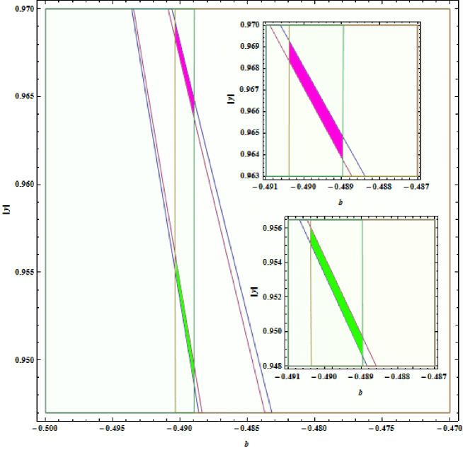
Figure 1: In this figure the whole region of the $|y|$-$b^{{}^{\prime}}$ plane which is allowed by our model is shown. The overlap region of the experimental values for $\frac{\Delta m_{21}^{2}}{\Delta m_{31}^{2}}$ and $\sin^{2}\theta_{13}$ with our model are two tiny regions close to the top left corner of the rectangular. In the zoomed box we have magnified the overlap regions. As mentioned in the text, only the lower overlap region is consistent with all of the experimental data.

First we check the consistency of the rest of the experimental data with the overlap region. We find that the upper overlap region is barely ruled out by the experimental value for $\sin^{2}\theta_{23}$, and the lower overlap region is consistent with all the rest. Having determined the unique overlap region, we can not only determine all of the parameters of our model, but also predict the masses of the neutrinos and the phases. The results for the parameters are as follows,

$$m_{0} \approx (3.3-3.7)10^{-2}eV,$$

$$a \approx -(1.71-1.93)10^{-2}eV,$$

$$b \approx -(1.61-1.81)10^{-2}eV,$$

$$B \approx (0.92-1.04)10^{-2}eV,$$

$$\lambda \approx -(1.98-2.96)10^{-4}eV.$$ (49)

By comparing the values of these parameters we conclude that the complexification part of the generalization of $M_{FL}$, accomplished by adding imaginary components denoted by B, could not be treated as a perturbation, while the second part of the generalization, accomplished by adding $\lambda S^{123}$, can indeed be treated as a perturbation. This is precisely what we have done.

Parameter	The exp. data	The best exp. fit($\pm 1\sigma$)	Predictions of our model
$\Delta m_{21}^{2}(10^{-5}eV^{2})$	$(7.12-8.20)$	$(7.43-7.81)$	$(7.12-7.84)$
$\Delta m_{31}^{2}(10^{-3}eV^{2})$	$(2.26-2.77)$	$(2.46-2.61)$	$(2.23-2.80)$
$\sin^{2}\theta_{12}$	$0.27-0.37$	$0.30-0.336$	$0.331-0.333$
$\sin^{2}\theta_{13}$	$0.016-0.037$	$0.0281-0.0275$	$0.0218-0.0275$
$\sin^{2}\theta_{23}$	$0.39-0.64$	$0.400-0.461$	$0.439-0.446$
		$0.573-0.635$
$\delta$	$...$	$...$	$59.21^{\circ}-59.34^{\circ}$
$\sigma=-\rho$	$...$	$...$	$59.44^{\circ}-59.51^{\circ}$
$|J|$	$...$	$...$	$0.029-0.033$
	$...$	$...$	$m_{1}\approx(0.031625-0.035687)eV,$
			$\langle m_{\nu_{e}}\rangle\approx(0.033-0.037)~{}eV$
masses	$...$	$...$	$m_{2}\approx(0.032732-0.036769)eV,$
			$\langle m_{\nu_{\mu}}\rangle\approx(0.043-0.048)~{}eV$
	$...$	$...$	$m_{3}\approx(0.056849-0.063819)eV,$
			$\langle m_{\nu_{\tau}}\rangle\approx(0.046-0.051)~{}eV$

Table 2: The available experimental data for neutrinos for the case of normal mass hierarchy and the predictions of our model. These predictions are obtained from our parameters as shown in Eq. (3). Specifically we have used $b^{{}^{\prime}}\approx-(0.489-0.4904)$ and $y\approx(0.948932-0.956141).$

Having determined all of the parameters of our model, we can compare our results with the experimental data. In Table 2 we state all of the relevant experimental data presented at $3\sigma$ [2], along with the predictions of our model. As shown in Table 2 we have predictions for some physical quantities for which no experimental data exist. We should mention at this point that if we had chosen $S^{123}$ instead of $S^{132}$ to break the $\mu-\tau$ symmetry and generate a nonzero value for $\theta_{13}$, all of our final results and prediction would be unaltered except for $J\rightarrow-J$.

An important experimental result for the sum of the three light neutrino masses has just been reported by the Planck measurements of the cosmic microwave background (CMB)[24], which is

$$\sum m_{\nu}<0.23eV\text{({Planck}+WP+highL+BAO),}$$ (50)

This sum in our model is $\sum m_{\nu}\approx(0.12-0.14)eV$, which is consistent with the above constraint. For the flavor eigenstates only the expectation values of the masses can be calculated and they are obtained by the following relation,

$$\langle m_{\nu_{i}}\rangle=\sum_{j=1}^{3}|U_{ij}|^{2}|m_{j}|,$$ (51)

where $i=e,\mu,~{}\text{and}~{}\tau$. Our predictions for these quantities are also shown in Table 2. The Majorana neutrinos can violate lepton number, for example in neutrinoless double beta decay $(0\nu\beta\beta)$ [25]. Such a process has not yet been observed and an upper bound has been set for the relevant quantity, i.e. $\langle m_{\nu_{ee}}\rangle$. Results from the first phase of the KamLAND-Zen experiment sets the following constraint $\langle m_{\nu_{ee}}\rangle<(0.12-0.25)~{}eV$ at $90\%$ CL [26]. Our prediction for this quantity is $\langle m_{\nu_{ee}}\rangle\approx(0.032-0.036)~{}eV$ which is consistent with the result of kamLAND-Zen experiment. We also predict $\langle m_{\nu_{e}}\rangle\approx(0.033-0.037)~{}eV$, $\langle m_{\nu_{\mu}}\rangle\approx(0.043-0.048)~{}eV$ and $\langle m_{\nu_{\tau}}\rangle\approx(0.046-0.051)~{}eV$.

4 Conclusions

In this paper we propose a generalized Friedberg-Lee neutrino mass model in which CP violation is possible. Our generalization consists of two steps. First we add imaginary components to the mass matrix, such that the resulting matrix is symmetric, magic with zero trace. The results is that $\mu-\tau$ symmetry is preserved and nonzero phases including $\delta$ are obtained. However, $\sin\theta_{13}$ remains zero. In the second stage we break the $\mu-\tau$ symmetry by adding a real matrix which is the matrix representation of the permutation group element $S^{(123)}$. This part is treated as a perturbation and a nonzero $\theta_{13}$ is generated. The combination of these two generalization then produces CP violation. We use self consistency arguments and the complementary ansatz to reduce our parameter space to two dimensions. Mapping two of the experimental data, i.e. the allowed ranges of $\sin^{2}\theta_{13}$ and $\frac{\Delta m^{2}_{21}}{\Delta m^{2}_{31}}$, onto our allowed region of the parameter space almost pinpoints the values of our parameters. We then check the consistency of all other experimental data with the allowed range. We then predict the mixing angles, the masses of neutrinos, the CP violation parameters $\delta$, $\rho$, $\sigma$, and $J$. All of our findings are shown in Table 2 along with the latest experimental values. As is evident from Table 2, all of our predictions are within the allowed ranges determined by the experiments and there is an excellent agreement between these values. Our predictions for the neutrino masses and CP violation parameters $\delta$ and $J$ are to tested by future experiments.

5 Acknowledgement

We would like to thank the research office of the Shahid Beheshti University for financial support.

References

- [1] SNO Collaboration, Q.R. Ahmad, et al., Phys. Rev. Lett. 89 (2002) 011301; For a review, see: C.K. Jung, et al., Annu. Rev. Nucl. Part. Sci. 51 (2001) 451; KamLAND Collaboration, K. Eguchi, et al., Phys. Rev. Lett. 90 (2003) 021802; K2K Collaboration, M.H. Ahn, et al., Phys. Rev. Lett. 90 (2003) 041801.
- [2] T. Schwetz, M. Tortola, J. W. F. Valle, New J. Phys., 13, 109401 (2011); D. V. Forero, M. T rtola, and J. W. F. Valle, Phys. Rev. D 86, 073012 (2012); F. P. An et al. (DAYA-BAY Collaboration), Phys. Rev. Lett. 108, 171803 (2012), arXiv:1203.1669v2 [hep-ex]; J.K. Ahn et al. (RENO Collaboration), Phys. Rev. Lett. 108, 191802 (2012); arXiv:1108.1376 [hep-ph].
- [3] D. V. Forero, M. T rtola, and J. W. F. Valle Phys. Rev. D 86, 073012 (2012), arXiv:1205.4018v2 [hep-ph].
- [4] J. Schechter and J. W. F. Valle Phys.Rev. D22 (1980) 2227; H. Fritzsch and Z.Z. Xing, Phys. Lett. B 517, 363 (2001). Particle Data Group, W.M. Yao et al., J. Phys. G 33, 1 (2006).
- [5] W. Rodejohann and J. W. F. Valle Phys.Rev. D84 (2011) 073011
- [6] P.F. Harrison, D.H. Perkins, W.G. Scott, Phys. Lett. B 530 (2002) 167.
- [7] P.H. Frampton, S.L. Glashow, D. Marfatia, Phys. Lett. B 536 (2002) 79; Z.Z. Xing, Phys. Lett. B 530 (2002) 159; Z.Z. Xing, Phys. Lett. B 539 (2002) 85; P.H. Frampton, M.C. Oh, T. Yoshikawa, Phys. Rev. D 66 (2002) 033007; A. Kageyama, et al., Phys. Lett. B 538 (2002) 96; B.R. Desai, D.P. Roy, A.R. Vaucher, Mod. Phys. Lett. A 18 (2003) 1355.
- [8] G.C. Branco, et al., Phys. Lett. B 562 (2003) 265.
- [9] See, e.g., W. Grimus, L. Lavoura, Phys. Rev. D 62 (2000) 093012; T. Asaka, et al., Phys. Rev. D 62 (2000) 123514; R. Kuchimanchi, R.N. Mohapatra, Phys. Rev. D 66 (2002) 051301; P.H. Frampton, S.L. Glashow, T. Yanagida, Phys. Lett. B 548 (2002) 119; T. Endoh, et al., Phys. Rev. Lett. 89 (2002) 231601; M. Raidal, A. Strumia, Phys. Lett. B 553 (2003) 72; B. Dutta, R.N. Mohapatra, hep-ph/0305059; N. Razzaghi, S. S. Gousheh, Phys. Rev. D 86, (2012) 053006.
- [10] D. Black, et al., Phys. Rev. D 62 (2000) 073015.
- [11] X.G. He, A. Zee, Phys.Rev. D68 (2003) 037302.
- [12] A. Zee, Phys. Lett. B 93 (1980) 389; A. Zee, Phys. Lett. B 95 (1980) 461, Erratum; L. Wolfenstein, Nucl. Phys. B 175 (1980) 93.
- [13] R.N. Mohapatra, G. Senjanovic, Phys. Rev. D 23 (1981) 165; C. Wetterich, Nucl. Phys. B 187 (1981) 343; J.C. Montero, C.A. de S. Pires, V. Pleitez, Phys. Lett. B 502 (2001) 167; R.N. Mohapatra, A. Perez-Lorenzana, C.A. de Sousa Pires, Phys. Lett. B 474 (2000) 355.
- [14] B. Bajc, G. Senjanovic, F. Vissani, hep-ph/0110310; B. Bajc, G. Senjanovic, F. Vissani, Phys. Rev. Lett. 90 (2003) 051802.
- [15] H.S. Goh, R.N. Mohapatra, S.P. Ng, Phys.Lett.B570:215-221,2003.
- [16] W. Rodejohann, Physics Letters B 579 (2004)127 139
- [17] R. Friedberg, T.D. Lee, High Energy Phys. Nucl. Phys. 30 (2006) 591; arXiv:hep-ph/0606071.
- [18] C. S. Huang, T. Li, W. Liao and S. H. Zhu, Phys. Rev. D 78, 013005 (2008).
- [19] Elizabeth Jenkins and Aneesh V. Manohar, Nucl. Phys. B792, 187 (2008).
- [20] C. Jarlskog, Phys. Rev. Lett. 55 (1985) 1039.
- [21] Z. Z. Xing, H. Zhang, S. Zhou, Phys Lett B 641 (2006) 189; T. Baba, M. Yasue, Phys. Rev. D75, 055001 (2007); Z. Z. Xing, H. Zhang, S. Zhou, Int. J. Mod. Phys. A 23, 3384(2008).
- [22] N. Razzaghi, S. S. Gousheh, Phys. Rev. D 86, (2012) 053006.
- [23] J. Schechter and J.W. F. Valle, Phys. Rev. D 22, 2227 (1980); Physics of neutrinos and applications to as- trophysics, Masataka Fukugita and Tsutomu Yanagida, Springer, (2003); S. Nasri, J. Schechter and S. Moussa , Phys. Rev. D 70, 053005(2004).
- [24] P. A. R. Ade et al.[Planck Collaboration], arXive:1303.5076v1.
- [25] S. P. Mikhyev and A. Y. Smirnov, Nuovo Cimento 9C, 17 (1986); L. Wolfenestein, Phys. Rev. D 17, 2369 (1978).
- [26] A. Gando et al. [KamLAND-Zen Collaboration], Phys. Rev. Lett. 110 (2013) 062502; arXiv:1211.3863v2.