A short survey on nonlinear models of the classic Costas loop:
rigorous derivation and limitations of the classic analysis.

Abstract

Rigorous nonlinear analysis of the physical model of Costas loop — a classic phase-locked loop (PLL) based circuit for carrier recovery, is a challenging task. Thus for its analysis, simplified mathematical models and numerical simulation are widely used. In this work a short survey on nonlinear models of the BPSK Costas loop, used for pre-design and post-design analysis, is presented. Their rigorous derivation and limitations of classic analysis are discussed. It is shown that the use of simplified mathematical models, and the application of non rigorous methods of analysis (e.g., simulation and linearization) may lead to wrong conclusions concerning the performance of the Costas loop physical model.

I INTRODUCTION

The Costas loop is a classic phase-locked loop (PLL) based circuit for carrier recovery [1, 2]. In this paper the classic analog Costas loop [1, 3], used for Binary Phase Shift Keying signals (BPSK) is considered. Costas loop is essentially a nonlinear control system and its physical model is described by a nonlinear non-autonomous system of discontinuous differential equations (mathematical model in the signal space), whose rigorous analytical is a difficult task. Thus, in practice, numerical simulation, simplified mathematical models, and linear analysis are widely used for the analysis of PLL based circuits (see, e.g., [4, 5, 3, 6, 7, 8]).

In the following it is shown that 1) the use of simplified mathematical models, and 2) the application of non rigorous methods of analysis (e.g., a simulation) may lead to wrong conclusions about the performance of the Costas loop physical model.

To demonstrate this, the operation of the Costas loop will be considered in details.

II Classical engineering consideration of the Costas loop operation

The operation of the Costas loop is considered first in the locked state (see Fig. 1), hence the frequency of the carrier is identical with the frequency of the VCO (Voltage-Controlled Oscillator); further it is assumed that both of these signals are sinusoidal.

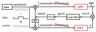
Figure 1: Costas loop is locked (the case of equal phases of input carrier and free running VCO output): there is no phase difference.

The input signal is a BPSK signal, which is the product of a transferred binary data ($m(t)\in\{\pm 1\}$ for any $t$) and the harmonic carrier $\sin(\omega t)$ with a high frequency $\omega$. Since the Costas loop is considered to be locked, the VCO output signal is synchronized with the carrier (i.e. there is no phase difference between these two signals). The input signal is multiplied (multiplier block ($\otimes$)) by the VCO signal on the upper branch and by the VCO signal, shifted by $90^{\circ}$, on the lower branch. Therefore on the multipliers’ outputs one has $\varphi_{1}(t)=\frac{1}{2}\big{(}m(t)-m(t)\cos(2\omega t)\big{)},\varphi_{2}(t)=\frac{1}{2}\big{(}m(t)\sin(2\omega t)\big{)}.$

Consider the low-pass filters (LPF1 and LPF2) operation.

Assumption 1

Signals components, whose frequency is about twice the carrier frequency, do not affect the synchronization of the loop (since they are completely suppressed by the low-pass filters).

Assumption 2

Initial states of the low-pass filters do not affect the synchronization of the loop (since for the properly designed filters, the impact of filter’s initial state on its output decays exponentially with time).

Assumption 3

The data signal $m(t)$ does not affect the synchronization of the loop.

Assumptions 1,2, and 3 together lead to the concept of so-called ideal low-pass filter, which completely eliminates all frequencies above the cutoff frequency (Assumption 1) while passing those below unchanged (Assumptions 2,3). In the classic engineering theory of the Costas loop it is assumed that the low-pass filters LPF1 and LPF2 are ideal low-pass filters.

Since in Fig. 1 the loop is in lock, i.e. the transient process is over and the synchronization is achieved, by Assumptions 1,2, and 3 for the outputs $g_{1,2}(t)$ of the low-pass filters LPF1 and LPF2 one has $g_{1}(t)=\frac{1}{2}m(t),\ g_{2}(t)=0.$ Thus, the upper branch works as a demodulator and the lower branch works as a phase-locked loop.

Since after a transient process there is no phase difference, a control signal at the input of VCO, which is used for VCO frequency adjustment to the frequency of input carrier signal, has to be zero: $g(t)=0$. In the general case when the carrier frequency $\omega$ and a free-running frequency $\omega_{\text{free}}$ of the VCO are different, after a transient processes the control signal at the input of VCO has to be non-zero constant: $g(t)=const$, and a constant phase difference $\theta_{\Delta}$ may remain.

Consider the Costas loop before synchronization (see Fig. 2). Here the phase difference $\theta_{\Delta}(t)=\theta_{1}(t)-\theta_{2}(t)$ varies over time, because the loop has not yet acquired lock (frequencies or phases of the carrier and VCO are different).

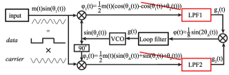
Figure 2: Costas loop is out of lock: there is time-varying phase difference.

In this case, using Assumption 1, the signals $\varphi_{1,2}(t)$ can be approximated as

$$\varphi_{1}(t)\approx\frac{1}{2}m(t)\cos(\theta_{\Delta}(t)), \varphi_{2}(t)\approx\frac{1}{2}m(t)\sin(\theta_{\Delta}(t)).$$ (1)

Approximations (1) depend on the phase difference of signals, i.e. two multiplier blocks ($\otimes$) on the upper and lower branches operate as phase detectors. The obtained expressions (1) with $m(t)\equiv 1$ coincide with well-known (see, e.g., [9, 3]) phase detector characteristic of the classic PLL with multiplier/mixer phase-detector for sinusoidal signals.

By Assumptions 2 and 3 the low-pass filters outputs can be approximated as

$$g_{1}(t)\approx\frac{1}{2}m(t)\cos(\theta_{\Delta}(t)), g_{2}(t)\approx\frac{1}{2}m(t)\sin(\theta_{\Delta}(t)).$$ (2)

For $m^{2}(t)\equiv 1$, the input of the loop filter is

$$\varphi(t)=g_{1}(t)g_{2}(t)\approx\varphi(\theta_{\Delta}(t))=\frac{1}{8}\sin(2\theta_{\Delta}(t)).$$ (3)

Such an approximation is called phase detector characteristic of the Costas loop.

Since an ideal low-pass filter is hardly realized, its use in the mathematical analysis requires additional justification.

Thus, the impact of the low-pass filters on the lock acquisition process must be studied rigorously. Also, the following caveats should be acknowledged.

Caveat to Assumption 1. While Assumption 1 is reasonable from a practical point of view, its use in the analysis of Costas loop requires further consideration (see, e.g., [10, 11]). Various averaging methods (see, e.g., [12]) allow one to justify Assumption 1 and obtain conditions under which it can be used rigorously (see [13, 14]).

Caveat to Assumption 2. Since in Fig. 2 the loop is out of lock, i.e. synchronization is not achieved, low-pass filters’ initial states cannot be ignored and must be taken into account. Therefore for rigorous consideration of low-pass filters influence one has to use a rigorous mathematical model of the low-pass filters instead of approximations (2). Since low-pass filter LPF2 is mostly used to indicate synchronization status and low-pass filter LPF1 is mostly used for data demodulation, the effect of nonzero initial state of filter on transient processes will be discussed below for the loop filter, which is used to provide synchronization.

Caveat to Assumption 3. The low-pass filters can not operate perfectly at the moments of changing $m(t)$, therefore the data pulse shapes are no longer ideal rectangular pulses after filtration. One known related effect is called false-locking: while for $m(t)\equiv const$ the loop acquires lock and proper synchronization of the carrier and VCO frequencies, for time-varying $m(t)\neq const$ the loop may seem to acquire lock without proper synchronization of the frequencies (false lock) [15, 16]. To avoid such undesirable situation one may try to choose loop parameters in such a way that the synchronization time is less than the time between changes in the data signal $m(t)$ or to modify the loop (see, e.g., [15]).

The relation between the input $\varphi(t)$ and the output $g(t)$ of the loop filter has the form

$$\dot{x}=Ax+b\varphi(t),\ g(t)=c^{*}x+h\varphi(t),$$ (4)

where $A$ is a constant matrix, the vector $x(t)$ is the loop filter state, $b,c$ are constant vectors, h is a number. The control signal $g(t)$ is used to adjust the VCO frequency to the frequency of the input carrier signal

$$\dot{\theta}_{2}(t)=\omega_{2}(t)=\omega_{2}^{\text{free}}+Lg(t).$$ (5)

Here $\omega_{2}^{free}$ is the free-running frequency of the VCO and $L$ is the VCO gain. The solution of (4) with initial data $x(0)$ (the loop filter output for the initial state $x(0)$) is as follows

$$\begin{array}[]{c}g(t,x(0))=\alpha_{0}(t,x(0))+\int\limits_{0}^{t}\gamma(t-\tau)\varphi(\tau){\rm d}\tau+h\varphi(t),\end{array}$$ (6)

where $\gamma(t-\tau)=c^{*}e^{A(t-\tau)}b+h$ is the impulse response of the loop filter and $\alpha_{0}(t,x(0))=c^{*}e^{At}x(0)$ is the zero input response of the loop filter, i.e. when the input of the loop filter is zero.

Assumption 4 (analog of Assumption 2)

Zero input of loop filter $\alpha_{0}(t,x(0))$ does not affect the synchronization of the loop (one of the reasons is that $\alpha_{0}(t,x(0))$ is an exponentially damped function for a stable matrix $A$).

Consider a constant frequency of the input carrier:

$$\dot{\theta}_{1}(t)=\omega_{1}(t)\equiv\omega_{1},$$ (7)

and introduce notation: $\omega_{\Delta}^{\text{free}}=\omega_{1}-\omega_{2}^{free}$. Then Assumption 4 allows one to obtain the classic mathematical model of PLL-based circuit in signal’s phase space (see the classic Viterbi’s book [9]):

$$\dot{\theta}_{\Delta}=\omega_{\Delta}^{\text{free}}-L\int_{0}^{t}\gamma(t-\tau)\varphi(\theta_{\Delta}(\tau)){\rm d}\tau-Lh\varphi(\theta_{\Delta}(t)).$$ (8)

Since $\varphi(\theta_{\Delta})$ from (3) is an odd function and has period $\pi$, one has $(\omega_{\Delta}^{\text{free}},\theta_{\Delta}(t))\rightarrow\big{(}-\omega_{\Delta}^{\text{free}},-\theta_{\Delta}(t))$ and $\theta_{\Delta}(t)\rightarrow\theta_{\Delta}(t)+\pi k$ do not change (8). Therefore in $\eqref{mathmodel-class-simple}$ one can consider only nonnegative $\omega_{\Delta}^{\text{free}}$ ($|\omega_{\Delta}^{\text{free}}|$ called frequency deviation) and $\theta_{\Delta}(0)\in[-\pi/2,\pi/2)$. The classic engineering task is to find the following sets: the hold-in range includes such $|\omega_{\Delta}^{\text{free}}|$ that (8) has a stationary state $\theta_{\Delta}(t)\equiv\theta^{eq}_{\Delta}$ which is locally stable (local stability, i.e. for some $\theta_{\Delta}(0)$); the pull-in range includes such $|\omega_{\Delta}^{\text{free}}|$ that any solution of (8) is attracted to one of the stationary state $\theta^{eq}_{\Delta}$ (global stability, i.e. for all $\theta_{\Delta}(0)$).

Caveat to Assumption 4. While Assumption 4 allows one to introduce one dimensional stability ranges, defined only by $|\omega_{\Delta}^{\text{free}}|$, $\alpha_{0}(t,x(0))$ may affect the synchronization of the loop and stability ranges. For rigorous study one has to consider multi-dimensional stability domains, taking into account $(\omega_{\Delta}^{\text{free}},x(0),x_{1}(0),x_{2}(0))$, and explain their relations with the classic engineering ranges [17] (e.g., it is of utmost importance for cycle slips study [18, 19] and lock-in range definition).

Note that while Assumption 2 is explained at the beginning Viterbi’s classical book [9] for the stable matrices $A$ only, further in the book, various filters with marginally stable matrices are also studied (e.g. filter – perfect integrator where $A=0$).

It is also interesting that for model $\eqref{mathmodel-class-simple}$ with $h=0$ (see, e.g., eq. (2.18) in [9]) the initial difference between frequencies $|\dot{\theta}_{\Delta}(0)|=|\omega_{\Delta}(0)|$ is equal to the frequency deviation $|\omega_{\Delta}^{\text{free}}|$. So these terms are often used in place of each other, which is not correct for $x(0)\neq 0$, $h\neq 0$ or a non odd function $\varphi(\theta_{\Delta})$.

While the classic model (8) may be useful at the stage of post-design analysis (when the input and the VCO output are considered only and the parameters are known only approximately), for the pre-design analysis (when all the parameters of the loop can be chosen precisely) one may use more informative models considered in the next sections.

III Nonlinear models of Costas loop

The relation between the inputs $\varphi_{1,2}(t)$ and the outputs $g_{1,2}(t)$ of linear low-pass filters is as follows

$$\dot{x}_{1,2}=A_{1,2}x_{1,2}+b_{1,2}\varphi_{1,2}(t),\ g_{1,2}(t)=c_{1,2}^{*}x_{1,2}.$$ (9)

Here $A_{1,2}$ are constant stable (all eigenvalues have negative real part) matrices, the vectors $x_{1,2}(t)$ are low-pass filters’ states, $b_{1,2}$ and $c_{1,2}$ are constant vectors, the vectors $x_{1,2}(0)$ are initial states of the low-pass filters. For the loop filter one can consider more the general equation (4) with a proportional term.

Taking into account (9), (4), and (5), one obtains the mathematical model in the signal space, describing the physical model of BPSK Costas loop,:

$$\dot{x}_{1}=A_{1}x_{1}+b_{1}m(t)\sin(\theta_{1}(t))\sin(\theta_{2}),$$ (10)

$$\dot{x}_{2}=A_{2}x_{2}+b_{2}m(t)\sin(\theta_{1}(t))\cos(\theta_{2}),$$

$$\dot{x}=Ax+b(c_{1}^{*}x_{1})(c_{2}^{*}x_{2}),$$

$$\dot{\theta}_{2}=\omega_{2}^{free}+L(c^{*}x)+Lh(c_{1}^{*}x_{1})(c_{2}^{*}x_{2}).$$

Note that Assumptions 1-4 are not used in the derivation of system (10).

The mathematical model in the signal space (10) is a nonlinear nonautonomous discontinuous differential system, so in general case its analytical study is a difficult task even for the continuous case when $m(t)\equiv const$. Besides it is a slow-fast system, so its numerical study (corresponding to the SPICE level simulation) is rather complicated for the high-frequency signals. The problem is that it is necessary to consider simultaneously both very fast time scale of the signals $\sin(\theta_{1,2}(t))$ and slow time scale of phase difference $\theta_{\Delta}(t)$, therefore a very small simulation time-step must be taken over a very long total simulation period [20].

To overcome these problems, in place of using Assumption 2 one can apply averaging methods [12, 14] and consider a simplified mathematical model in signal’s phase space. However, this requires the consideration of a constant data signal (Assumption 3) and constant frequency of input carrier (7), i.e.

$$m(t)\equiv 1,\quad\theta_{1}(t)=\omega_{1}t+\theta_{1}(0).$$

In this case (10) is equivalent to

$$\dot{x_{1}}=A_{1}x_{1}+b_{1}\sin(\omega_{1}t+\theta_{1}(0))\sin(\omega_{1}t+\theta_{1}(0)+\theta_{\Delta}),$$ (11)

$$\dot{x_{2}}=A_{2}x_{2}+b_{2}\sin(\omega_{1}t+\theta_{1}(0))\cos(\omega_{1}t+\theta_{1}(0)+\theta_{\Delta}),$$

$$\dot{x}=Ax+b(c_{1}^{*}x_{1})(c_{2}^{*}x_{2}),$$

$$\dot{\theta}_{\Delta}=\omega_{\Delta}^{\text{free}}-L(c^{*}x)-Lh(c_{1}^{*}x_{1})(c_{2}^{*}x_{2}).$$

Here the initial (at $t=0$) difference of the frequencies has the form

$$\dot{\theta}_{\Delta}(0)=\omega_{\Delta}(0)=\omega_{\Delta}^{\text{free}}-Lc^{*}x(0)-Lhc_{1}^{*}x_{1}(0)c_{2}^{*}x_{2}(0).$$ (12)

Assuming that the input carrier is a high-frequency signal (i.e. $\omega_{1}>\omega_{min}$ is sufficiently large), one can consider small parameter $\varepsilon=\frac{1}{\omega_{1}}$. Denote $\tau=\omega_{1}t$. Then system (11) can be represented in the following way

$$\frac{dz}{d\tau}=\varepsilon F(z,\tau),\quad z=(x_{1},x_{2},x,\theta_{\Delta})^{*}.$$ (13)

Consider the averaged equation (13)

$$\frac{dy}{d\tau}=\varepsilon\bar{F}(y),\ \bar{F}(y)=\frac{1}{2\pi}\int_{0}^{2\pi}F(y,\tau)d\tau.$$ (14)

Suppose, $D$ is a bounded domain, containing the point $z_{0}=(x_{1}(0),x_{2}(0),x(0),\theta_{\Delta}(0))$. Consider solutions $z(\tau,\varepsilon)$ and $y(\tau,\varepsilon)$ with the initial data $z_{0}=y_{0}$. In this case there exists a constant $T$ such that $z(\tau,\varepsilon)$ and $y(\tau,\varepsilon)$ remain in the domain $D$ for $0\leq\tau\leq\frac{T}{\varepsilon}$. Define $\varepsilon_{max}=\frac{1}{\omega^{min}}$.

Theorem 1

[12] Suppose that $\varepsilon_{max}$, $D$, and $T$ are as above. Then there exists a constant $c>0$ such that $||y(t,\varepsilon)-z(t,\varepsilon)||<c\varepsilon$ for $0\leq\varepsilon\leq\varepsilon_{max}$ and $0\leq t\leq\frac{T}{\varepsilon}$.

Remark. Time $T$ has to be defined by the time of the transient processes. The theorem does not suggest how to define $T$ by the loop parameters, so $T$ is supposed to be estimated experimentally. Also note that the averaged system can be considered only if

$$0<\omega^{min}\leq\omega_{1},\omega_{2}(t),$$ (15)

$$|\omega_{1}-\omega_{2}(t)|\leq\omega^{max}_{\Delta}\quad\forall t\in[0,T],$$

where $\omega^{max}_{\Delta}$ does not depend on $\omega^{min}$ and $\omega^{min}$ is sufficiently large.

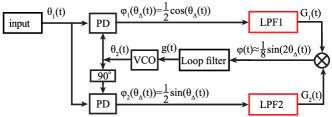
Figure 3: Mathematical model of BPSK Costas loop in signal’s phase space

In this case the averaged system (14) gives a mathematical model of BPSK Costas loop in signal’s phase space (see Fig. 3):

$$\dot{x_{1}}=A_{1}x_{1}+\frac{b_{1}}{2}\cos(\theta_{\Delta}),\quad\dot{x_{2}}=A_{2}x_{2}+\frac{b_{2}}{2}\sin(\theta_{\Delta}),$$ (16)

$$\dot{x}=Ax+b(c_{1}^{*}x_{1})(c_{2}^{*}x_{2}),$$

$$\dot{\theta}_{\Delta}=\omega_{\Delta}^{\text{free}}-L(c^{*}x)-Lh(c_{1}^{*}x_{1})(c_{2}^{*}x_{2}).$$

Here, under condition (15), Theorem 1 provides the closeness solutions of averaged (16) and original (10) systems. Remark that in (16) the initial difference between frequencies $\omega_{\Delta}(0)$ coincides with (12).

Mathematical model (16) does not coincide with that, considered in the classic works [2, 9]. The classical mathematical model of the Costas loop can be obtained from this model under additional assumptions.

III-A Classical model of BPSK Costas loop

Having solved the first two equations of system (16), one obtains

$\begin{aligned} &c_{1}^{*}x_{1}=\alpha_{1}(t,x_{1}(0))+\int_{0}^{t}\gamma_{1}(t-\tau)\frac{1}{2}\cos(\theta_{\Delta}(\tau))d\tau,\\ &c_{2}^{*}x_{2}=\alpha_{2}(t,x_{2}(0))+\int_{0}^{t}\gamma_{2}(t-\tau)\frac{1}{2}\sin(\theta_{\Delta}(\tau))d\tau.\\ \end{aligned}$

Here the impact of filter’s initial state on its output decays exponentially with time (see Assumption 2) and one can consider $t>t_{0}$, such that $\alpha_{1,2}(t,x_{1,2}(0))=O(\frac{1}{\omega^{min}})$.

Since the low-pass filters LPF1 and LPF2 are assumed to be ideal (see Assumptions 1-2), under conditions (15) their operation can be formalized as

$$\int_{t_{0}}^{t}\gamma_{1,2}(t-\tau)\sin(\theta_{\Delta}(\tau))d\tau=\sin\big{(}\theta_{\Delta}(t)\big{)}+O(\frac{1}{\omega^{min}}).$$

Then for $t>t_{0}$ one has

$$c_{1}^{*}x_{1}(t)=\dfrac{1}{2}\cos\big{(}\theta_{\Delta}(t)\big{)}+O(\frac{1}{\omega^{min}}),$$ (17)

$$c_{2}^{*}x_{2}(t)=\dfrac{1}{2}\sin\big{(}\theta_{\Delta}(t)\big{)}+O(\frac{1}{\omega^{min}}).$$

Applying (17) to (16), for $t>t_{0}$ one obtains

$$\dot{x}=Ax+b\frac{1}{8}\sin(2\theta_{\Delta})+O(\frac{1}{\omega^{min}}),$$ (18)

$$\dot{\theta}_{\Delta}=\omega_{\Delta}^{\text{free}}-Lc^{*}x-Lh\frac{1}{8}\sin(2\theta_{\Delta})-O(\frac{1}{\omega^{min}}).$$

Assumption 5 (Corollary of Assumptions 1-3))

Solutions of system (16) are close to solutions of the following system

$$\dot{x}=Ax+b\varphi(\theta_{\Delta}),$$ (19)

$$\dot{\theta}_{\Delta}=\omega_{\Delta}^{\text{free}}-Lc^{*}x-Lh\varphi(\theta_{\Delta}),$$

i.e. $O(\frac{1}{\omega^{min}})$ in system (16) can be neglected.

Figure 4: Classical (simplified) mathematical model of BPSK Costas loop in signal’s phase space

System (19) corresponds to the block-diagram shown in Fig. 4, where $\varphi(\theta_{\Delta})$ is the phase detector characteristic of the Costas loop for sinusoidal signals. Note that here the phase detector operation includes the operations of three multipliers, phase shift element $90^{\circ}$, LPF1, and LPF2. System (19) with $h=0$ and $x(0)=0$ corresponds to system (8).

Caveat to Assumption 5. For rigorous justification of Assumption 5 one may analyze stability conditions for system (19) (see, e.g., criteria of stability in the large for the pendulum-like systems [17]).

In some applications a modification of the BPSK Costas loop, shown in Fig. 5, is used. Here low-pass filters LPF1 and LPF2 do not affect the operation of the modified BPSK Costas loop (i.e. Assumption 2 is not needed); the input of the loop filter does not depend on the data signal $m(t)$ (i.e. Assumption 3 is not needed):

$\varphi(t)=\varphi_{1}(t)\varphi_{2}(t)=\sin(\theta_{1}(t))\sin(\theta_{2}(t))\sin(\theta_{1}(t))\cos(\theta_{2}(t))$.

Figure 5: A modification of BPSK Costas loop

Taking into account (4) and (5), one obtains a mathematical model in the signal space describing the physical model of modified BPSK Costas loop:

$$\dot{x}=Ax+b\varphi(t),\quad\dot{\theta}_{\Delta}=\omega_{\Delta}^{\text{free}}-Lc^{*}x-Lh\varphi(t).$$ (20)

The averaged system (20) gives a mathematical model of modified BPSK Costas loop in signal’s phase space (see Fig. 4) which corresponds to (19). Here, under condition (15), from Theorem 1 it follows that the solutions of systems (20) and (19) are close. The approach suggested in [21, 13, 22, 14] allows one to find an approximation $\varphi(\theta_{\Delta})$ in the case of non-constant frequency of the carrier or non sinusoidal signals.

IV Summary of the models

• physical model (with data signal and low-pass filters) or its mathematical model in the signal space (Fig. 2 or Fig. 6 and system (10));

• simplified mathematical model in the signal space (without data signal and with low-pass filters)) (system (11) and Fig. 2 or Fig. 6 with $m(t)\equiv 1$);

• modified physical model (with data signal and with external low-pass filters) or its mathematical model in the signal space (Fig. 5 and system (20));

• simplified mathematical model in signal’s phase space (without data signal and with low-pass filters) (system (16) and Fig. 3);

• classic mathematical model in signal’s phase space (without data signal and without low-pass filters) (system (19) and Fig. 4).

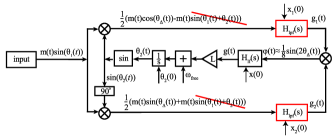
Figure 6: Block-diagram of Costas loop mathematical model in the signal space described by transfer functions and initial conditions

V Costas loop simulation and counterexamples to the Assumptions

Note once more that various simplifications and analysis of linearized models of control systems may result in incorrect conclusions. At the same time the attempts to justify analytically the reliability of conclusions, based on engineering approaches, and rigorous study of nonlinear models are quite rare (see, e.g., tutorial [23]).

Further it is demonstrated that the use of the above engineering Assumptions requires further study and rigorous justification. Next examples shows that for the same parameters the behaviors of considered models may be substantially different from one another.

V-A Simulation examples

Next the following parameters are used in simulation: low-pass filters transfer functions $H_{lpf}(s)=\frac{2}{s/\omega_{3}+1}$, $\omega_{3}=1.2566*10^{6}$ and corresponding parameters in system (4) are $A_{1,2}=-\omega_{3}$, $b_{1,2}=1$, $c_{1,2}=\omega_{3}$; loop filter transfer function $H_{lf}(s)=\frac{\tau_{2}s+1}{\tau_{1}s}$, $\tau_{2}=3.9789*10^{-6}$, $\tau_{1}=2*10^{-5}$, and corresponding parameters in system (4) are $A=0$, $b=1$, $c=\frac{1}{\tau_{1}}$, $h=\frac{\tau_{2}}{\tau_{1}}$; carrier frequency $\omega_{1}=2*\pi*400000$; VCO input gain $L=4.8*10^{6}$; and carrier initial phase $\theta_{2}(0)=\theta_{1}(0)=0$.

Example 1 (double frequency and averaging)

In Fig. 7 it is shown that Assumption 1 may not be valid if conditions for the application of Theorem 1 are violated: mathematical model signal’s phase space (see Fig. 3, system (16)) (black color) and physical model (see Fig. 6, system (10)) (red color) after transient processes have different phases in the locked states.

Here VCO free-running frequency $\omega_{2}^{free}=2*\pi*400000-600000$; initial states of filters are all zero: $x(0)=x_{1}(0)\equiv x_{2}{0}=0$ (i.e. $\alpha_{0}(t,x(0))=\alpha_{1,2}(t,x_{1,2}(0))\equiv 0$).

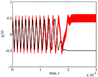
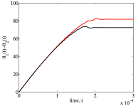
Figure 7: Low-pass filter outputs $g_{1}(t)$ and phase difference $\theta_{\Delta}(t)$ for averaged model (16) (black) and physical model (red) in Fig. 2.

Example 2 (initial states of the low-pass filters)

In Fig. 8 it is shown that Assumption 2 may not be valid: while physical model (see Fig. 6, system (10)) with zero initial states of low-pass filters acquires lock (black), the same physical model with nonzero initial states of low-pass filters is out of lock (red).

Here VCO free-running frequency $\omega_{2}^{free}=2*\pi*400000-2$, initial state of the loop filter is zero: $x(0)=0$ (i.e. $\alpha_{0}(t,x(0))\equiv 0$), Initial states of the low-pass filters are $x_{1}(0)=x_{2}(0)=0$ (black) and $x_{1}(0)=0.02$, $x_{2}(0)=0$ (red).

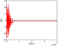
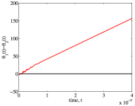
Figure 8: Loop filter output $g(t)$ for physical model (black) with zero initial states of low-pass filters, physical model (red) with nonzero initial states of low-pass filters.

Example 3 (data signal)

In Fig. 9 it is shown that Assumption 3 may not be valid: while the simplified mathematical model in the signal space (see Fig. 6 with $m(t)\equiv 1$, system (11)) acquires lock (black), physical model with (see Fig. 6, system (10)) with periodic data is out of lock (red).

Here VCO free-running frequency $\omega_{2}^{free}=3.2*10^{6}$, initial states of filters are all zero: $x(0)=x_{1}(0)=x_{2}(0)=0$, data signal is periodic: $m(t)=\operatorname{sign}\sin(10^{5}*2*\pi*t)$.

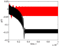
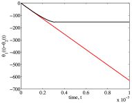
Figure 9: Loop filter output $g(t)$ for physical model (red) with periodic data signal, physical model (black) with constant data signal $m(t)\equiv 1$.

Example 4 (low-pass filters)

In Fig. 10 it is shown that the consideration of the ideal low-pass filters (Assumptions 1,2, and 3) may lead to wrong conclusions: it is shown that low-pass filters may affect the stability of models in signal’s phase space. While simplified mathematical model in signal’s phase space (see Fig. 3, system (16)) (black) and simplified mathematical model in the signal space (see Fig. 6 with $m(t)\equiv 1$, system (11)) (green) are out of lock, the classic mathematical model in signal’s phase space (see Fig. 4, system (19)), where low-pass filters are not taken into account, acquires lock (red).

Here VCO free-running frequency $\omega_{2}^{free}=2*\pi*400000-500000$, initial states of filters are zero: $x(0)=x_{1}(0)=x_{2}(0)=0$, no data is being transmitted: $m(t)\equiv 1$.

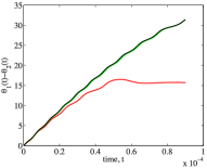
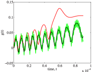
Figure 10: Loop filter output $g(t)$ and phase difference $\theta_{\Delta}(t)$ for signal’s phase space model (black) with low-pass filters, classic signal’s phase space model (red) without low-pass filters, and signal space model (green).

Example 5 (initial state of the loop filter)

In Fig. 11 it is shown that Assumption 4 may not be valid: while the physical model (see Fig. 6, system (10)) with zero output of loop filter acquires lock (black), the same physical model with nonzero output of loop filter is out of lock (red).

Here initial states of low-pass filters are zero: $x_{1}(0)=x_{2}(0)=0$; VCO free-running frequency $\omega_{2}^{free}=2*\pi*400000-10$; initial loop filter state is $x(0)=-0.00001$ (red) and $x(0)=0$ (black).

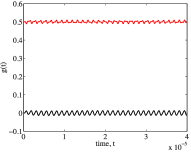
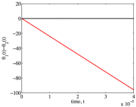
Figure 11: Loop filter output $g(t)$ and phase difference $\theta_{\Delta}(t)$ for physical model with zero initial state of loop filter (black), physical model with nonzero initial state of loop filter (red).

Example 6 (numerical integration parameters)

In Fig. 12 it is shown that standard simulation of the loop may not be valid: while the classic mathematical model in signal’s phase space (Fig. 4 or system (19)), simulated in Simulink with predefined integration parameters: ’max step size’ set to ’1e-3’, is out of lock (black), the same model simulated in Simulink with default integration parameters: ’max step size’ set to ’auto’, acquires lock (red). Here Matlab chooses step from $5\cdot 10^{-3}$ to $9\cdot 10^{-2}$; for fixed step $2\cdot 10^{-2}$ the model acquires lock, for fixed step $1\cdot 10^{-2}$ the model doesn’t acquire lock.

Here the initial loop filter state output is $x(0)=0.0125$; VCO free-running frequency $\omega_{2}^{free}=10000-89.45$; VCO input gain $L=1000$; initial phase shift $\theta_{\Delta}(0)=-3.4035$.

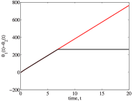
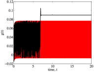
Figure 12: Filter outputs: default integration parameters in Simulink ’max step size’ set to ’auto’ (black curve); Parameters configured manually ’max step size’ set to ’1e-3’ (red curve).

Consider now the corresponding phase portrait (see Fig. 13).

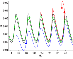
Figure 13: Phase portrait: coexistence of stable and unstable periodic solutions.

Here the red trajectory tends to a stable equilibrium (red dot). Lower and higher black trajectories are stable and unstable limit cycles. The blue trajectory tends to a stable periodic trajectory (lower black periodic curve) and in this case the model does not acquire lock. All trajectories between black trajectories (see green trajectory) tend to the stable lower black trajectory.

If the gap between stable and unstable trajectories (black lines) is smaller than the discretization step, the numerical procedure may slip through the stable trajectory (blue trajectory may step over the black and green lines and begins to be attracted to the red dot). In other words, the simulation may show that the Costas loop acquires lock although in reality it does not. The considered case corresponds to the coexisting attractors (one of which is a hidden oscillation) and the bifurcation of birth of a semistable trajectory [24].

Note, that only trajectories (red) above the unstable limit cycle is attracted to the equilibrium. Hence $\omega_{\Delta}=89.45$ does not belong to the pull-in range.

VI Conclusion

In this paper a short survey on derivation of nonlinear mathematical models of BPSK Costas loop, used for pre-design and post-design analysis, is presented. It has been shown that 1) the consideration of simplified mathematical models, constructed intuitively, and 2) the application of non rigorous methods of analysis (e.g., simulation and linearization) can lead to wrong conclusions concerning the operability of the Costas loop physical model. Similar result can be obtained for the classic PLL and QPSK Costas loop (see, e.g., [25, 11, 26]).

While the Costas loop is a nonlinear control system and for its analysis it is essential to apply various stability criteria developed in the control theory, their direct application to the PLL-based models is impossible, because such criteria usually are not adapted for the cylindrical phase space. In the tutorial Phase Locked Loops: a Control Centric Tutorial, presented at the American Control Conference 2002, D. Abramovitch wrote that “The general theory of PLLs and ideas on how to make them even more useful seems to cross into the controls literature only rarely” [23].

Corresponding modifications of the classic stability criteria for the rigorous analytical analysis of nonlinear PLL-based model in the cylindrical phase space had been well developed in 197x-199x in [27, 28, 29]. See also some recent works on nonlinear methods for the analysis of PLL-based models [30, 31, 32, 33, 34, 35, 36, 17]. One of the reason why these works have been remained almost unnoticed by the engineers may be that they are mostly written in the language of the control theory and the theory of dynamical systems, and, thus, may not be well adapted to the terms and objects used in the engineering practice of phase-locked loops. Another possible reason is that  “nonlinear analysis techniques are well beyond the scope of most undergraduate courses in communication theory” [7].

The examples, considered in the paper, are the motivation to apply rigorous analytical methods for the analysis of PLL-based loop nonlinear models.

References

- [1] J. Costas, “Synchoronous communications,” in Proc. IRE, vol. 44, 1956, pp. 1713–1718.
- [2] J. P. Costas, “Receiver for communication system,” July 1962, US Patent 3,047,659.
- [3] R. Best, Phase-Lock Loops: Design, Simulation and Application, 6th ed. McGraw-Hill, 2007.
- [4] M. Kihara, S. Ono, and P. Eskelinen, Digital Clocks for Synchronization and Communications. Artech House, 2002.
- [5] G. Bianchi, Phase-Locked Loop Synthesizer Simulation. McGraw-Hill, 2005.
- [6] D. Pederson and K. Mayaram, Analog Integrated Circuits for Communication: Principles, Simulation and Design. Springer, 2008.
- [7] W. Tranter, T. Bose, and R. Thamvichai, Basic Simulation Models of Phase Tracking Devices Using MATLAB, ser. Synthesis lectures on communications. Morgan & Claypool, 2010.
- [8] D. Talbot, Frequency Acquisition Techniques for Phase Locked Loops. Wiley, 2012.
- [9] A. Viterbi, Principles of coherent communications. New York: McGraw-Hill, 1966.
- [10] J. Piqueira and L. Monteiro, “Considering second-harmonic terms in the operation of the phase detector for second-order phase-locked loop,” IEEE Transactions On Circuits And Systems-I, vol. 50, no. 6, pp. 805–809, 2003.
- [11] N. Kuznetsov, O. Kuznetsova, G. Leonov, P. Neittaanmaki, M. Yuldashev, and R. Yuldashev, “Limitations of the classical phase-locked loop analysis,” in International Symposium on Circuits and Systems (ISCAS). IEEE, 2015, accepted.
- [12] Y. Mitropolsky and N. Bogolubov, Asymptotic Methods in the Theory of Non-Linear Oscillations. New York: Gordon and Breach, 1961.
- [13] G. A. Leonov, N. V. Kuznetsov, M. V. Yuldahsev, and R. V. Yuldashev, “Analytical method for computation of phase-detector characteristic,” IEEE Transactions on Circuits and Systems - II: Express Briefs, vol. 59, no. 10, pp. 633–647, 2012.
- [14] G. A. Leonov, N. V. Kuznetsov, M. V. Yuldashev, and R. V. Yuldashev, “Nonlinear dynamical model of Costas loop and an approach to the analysis of its stability in the large,” Signal processing, vol. 108, pp. 124–135, 2015.
- [15] M. Olson, “False-lock detection in Costas demodulators,” Aerospace and Electronic Systems, IEEE Transactions on, vol. AES-11, no. 2, pp. 180–182, 1975.
- [16] J. Stensby, “False lock and bifurcation in Costas loops,” SIAM Journal on Applied Mathematics, vol. 49, no. 2, pp. pp. 420–431, 1989.
- [17] G. A. Leonov and N. V. Kuznetsov, Nonlinear Mathematical Models Of Phase-Locked Loops. Stability and Oscillations. Cambridge Scientific Press, 2014.
- [18] G. Ascheid and H. Meyr, “Cycle slips in phase-locked loops: A tutorial survey,” Communications, IEEE Transactions on, vol. 30, no. 10, pp. 2228–2241, 1982.
- [19] O. B. Ershova and G. A. Leonov, “Frequency estimates of the number of cycle slidings in phase control systems,” Avtomat. Remove Control, vol. 44, no. 5, pp. 600–607, 1983.
- [20] P. Goyal, X. Lai, and J. Roychowdhury, “A fast methodology for first-time-correct design of PLLs using nonlinear phase-domain VCO macromodels,” in Proceedings of the 2006 Asia and South Pacific Design Automation Conference, 2006, pp. 291–296.
- [21] N. V. Kuznetsov, G. A. Leonov, M. V. Yuldashev, and R. V. Yuldashev, “Analytical methods for computation of phase-detector characteristics and PLL design,” in ISSCS 2011 - International Symposium on Signals, Circuits and Systems, Proceedings. IEEE, 2011, pp. 7–10.
- [22] N. V. Kuznetsov, G. A. Leonov, P. Neittaanmaki, M. V. Yuldashev, and R. V. Yuldashev, “Method and system for modeling Costas loop feedback for fast mixed signals,” Finland Patent, 2013, Patent application FI20130124.
- [23] D. Abramovitch, “Phase-locked loops: A control centric tutorial,” in American Control Conf. Proc., vol. 1, 2002, pp. 1–15.
- [24] G. A. Leonov and N. V. Kuznetsov, “Hidden attractors in dynamical systems. From hidden oscillations in Hilbert-Kolmogorov, Aizerman, and Kalman problems to hidden chaotic attractors in Chua circuits,” International Journal of Bifurcation and Chaos, vol. 23, no. 1, 2013, art. no. 1330002.
- [25] N. Kuznetsov, G. Leonov, M. Yuldashev, and R. Yuldashev, “Nonlinear analysis of classical phase-locked loops in signal’s phase space,” IFAC Proceedings Volumes (IFAC-PapersOnline), vol. 19, no. 1, pp. 8253–8258, 2014.
- [26] N. Kuznetsov, O. Kuznetsova, G. Leonov, P. Neittaanmaki, M. Yuldashev, and R. Yuldashev, “Simulation of nonlinear models of QPSK Costas loop in Matlab Simulink,” in Ultra Modern Telecommunications and Control Systems and Workshops (ICUMT), 2014 6th International Congress on. IEEE, 2014, pp. 66–71.
- [27] A. Gelig, G. Leonov, and V. Yakubovich, Stability of Nonlinear Systems with Nonunique Equilibrium (in Russian). Nauka, 1978.
- [28] G. A. Leonov, V. Reitmann, and V. B. Smirnova, Nonlocal Methods for Pendulum-like Feedback Systems. Stuttgart-Leipzig: Teubner Verlagsgesselschaft, 1992.
- [29] G. A. Leonov, I. M. Burkin, and A. I. Shepelyavy, Frequency Methods in Oscillation Theory. Dordretch: Kluwer, 1996.
- [30] A. Suarez and R. Quere, Stability Analysis of Nonlinear Microwave Circuits. Artech House, 2003.
- [31] V. A. Yakubovich, G. A. Leonov, and A. K. Gelig, Stability of Stationary Sets in Control Systems with Discontinuous Nonlinearities. Singapure: World Scientific, 2004.
- [32] N. Margaris, Theory of the Non-Linear Analog Phase Locked Loop. New Jersey: Springer Verlag, 2004.
- [33] G. A. Leonov, “Phase-locked loops. Theory and application,” Automation and Remote Control, vol. 10, pp. 47–55, 2006.
- [34] J. Kudrewicz and S. Wasowicz, Equations of phase-locked loop. Dynamics on circle, torus and cylinder. World Scientific, 2007.
- [35] C. Chicone and M. Heitzman, “Phase-locked loops, demodulation, and averaging approximation time-scale extensions,” SIAM J. Applied Dynamical Systems, vol. 12, no. 2, pp. 674–721, 2013.
- [36] G. A. Leonov, N. V. Kuznetsov, and S. M. Seledzhi, Automation control - Theory and Practice. In-Tech, 2009, ch. Nonlinear Analysis and Design of Phase-Locked Loops, pp. 89–114.