Hold-in, pull-in, and lock-in ranges of PLL circuits: rigorous mathematical definitions
and limitations of classical theory.

Abstract

The terms hold-in, pull-in (capture), and lock-in ranges are widely used by engineers for the concepts of frequency deviation ranges within which PLL-based circuits can achieve lock under various additional conditions. Usually only non-strict definitions are given for these concepts in engineering literature. After many years of their usage, F. Gardner in the 2nd edition of his well-known work, Phaselock Techniques, wrote “There is no natural way to define exactly any unique lock-in frequency” and “despite its vague reality, lock-in range is a useful concept”. Recently these observations have led to the following advice given in a handbook on synchronization and communications “We recommend that you check these definitions carefully before using them”[1, p.49]. In this survey an attempt is made to discuss and fill some of the gaps identified between mathematical control theory, the theory of dynamical systems and the engineering practice of phase-locked loops. It is shown that, from a mathematical point of view, in some cases the hold-in and pull-in “ranges” may not be the intervals of values but a union of intervals and thus their widely used definitions require clarification. Rigorous mathematical definitions for the hold-in, pull-in, and lock-in ranges are given. An effective solution for the problem on the unique definition of the lock-in frequency, posed by Gardner, is suggested.

I Introduction

The phase-locked loop based circuits (PLL) are widely used in various applications. A PLL is essentially a nonlinear control system and its nonlinear analysis is a challenging task. Much engineering writing is devoted to the study of PLL-based circuits and the various characteristics for their stability (see, e.g. a rather comprehensive bibliography of pioneering works in [2]). An important engineering characteristic of PLL is a set of parameters’ values for which a PLL achieves lock. In the classical books on PLLs [3, 4, 5], published in 1966, such concepts as hold-in, pull-in, lock-in, and other frequency ranges for which PLL can achieve lock, were introduced. They are widely used nowadays (see, e.g. contemporary engineering literature [6, 7, 8] and other publications). Usually in engineering literature only non-strict definitions are given for these concepts. F. Gardner in 1979 in the 2nd edition of his well-known work, Phaselock Techniques, formulated the following problem [9, p.70] (see also the 3rd edition [6, p.187-188]): “There is no natural way to define exactly any unique lock-in frequency”. The lack of rigorous explanations led to the paradox: “despite its vague reality, lock-in range is a useful concept” [9, p.70]. Many years of using definitions based on the above concepts has led to the advice given in a handbook on synchronization and communications, namely to check the definitions carefully before using them [1, p.49].

In this paper it is shown that, from a mathematical point of view, in some cases the hold-in and pull-in “ranges” may be not intervals of values but a union of intervals, and thus their widely used definitions require clarification. Next, rigorous mathematical definitions for the hold-in, pull-in, and lock-in ranges are given. In addition we suggest an effective solution for the problem of the unique definition of the lock-in frequency, posed by Gardner.

II Classical nonlinear mathematical models of PLL-based circuits in a signal’s phase space

In classical engineering publications various analog PLL-based circuits are represented in a signal’s phase space (also named frequency-domain [10, p.338]) by the block diagram shown in Fig. 1.

Figure 1: PLL-based circuit in a signal’s phase space.

Considering the corresponding mathematical model: the Phase Detector (PD) is a nonlinear block; the phases $\theta_{1,2}(t)$ of the input (reference) and VCO signals are PD block inputs and the output is a function $\varphi(\theta_{\Delta}(t))=\varphi(\theta_{1}(t)-\theta_{2}(t))$ named a phase detector characteristic, where

$$\theta_{\Delta}(t)=\theta_{1}(t)-\theta_{2}(t),$$ (1)

named the phase error. The relationship between the input $\varphi(\theta_{\Delta}(t))$ and the output $g(t)$ of the linear filter (Loop filter) is as follows:

$$\dot{x}=Ax+b\varphi(\theta_{\Delta}(t)),\ g(t)=c^{*}x+h\varphi(\theta_{\Delta}(t)),$$ (2)

where $A$ is a constant matrix, $x(t)\in\mathbb{R}^{n}$ the filter state, $x(0)$ the initial state of filter, $b$ and $c$ constant vectors, and h a number. The filter transfer function has the form:

$$H(s)=-c^{*}(A-sI)^{-1}b+h.$$ (3)

A lead-lag filter [7] (usually $H(0)=-c^{*}A^{-1}b+h=1$, but $H(0)$ can also be any nonzero value when an active lead-lag filter is used), or a PI filter ($H(0)$ is infinite) is usually used as the filter. The solution of (2) with initial data $x(0)$ (the filter output for the initial state $x(0)$) is as follows:

$$\begin{array}[]{c}g(t,x_{0})=\alpha_{0}(t,x(0))+\int\limits_{0}^{t}\gamma(t-\tau)\varphi(\theta_{\Delta}(\tau)){\rm d}\tau+h\varphi(\theta_{\Delta}(t)),\end{array}$$ (4)

where $\gamma(t-\tau)=c^{*}e^{A(t-\tau)}b$ is the impulse response function of the filter and $\alpha_{0}(t,x(0))=c^{*}e^{At}x(0)$ the zero input response (natural response, i.e. when the input of the filter is zero). The control signal $g(t)$ adjusts the VCO frequency to the frequency of the input signal:

$$\dot{\theta}_{2}(t)=\omega_{2}(t)=\omega_{2}^{\text{free}}+Lg(t),$$ (5)

where $\omega_{2}^{\text{free}}$ is the VCO free-running frequency (i.e. for $g(t)\equiv 0$) and $L$ the VCO gain. Nonlinear VCO models can be similarly considered, see, e.g. [12, 13]. The frequency of the input signal (reference frequency) is usually assumed to be constant:

$$\dot{\theta}_{1}(t)=\omega_{1}(t)\equiv\omega_{1}.$$ (6)

The difference between the reference frequency and the VCO free-running frequency is denoted as $\omega_{\Delta}^{\text{free}}$:

$$\omega_{\Delta}^{\text{free}}\equiv\omega_{1}-\omega_{2}^{\text{free}}.$$ (7)

By combining equations (1), (2), and (5)–(7) a nonlinear mathematical model in the signal’s phase space is obtained (i.e. in the state space: the filter’s state $x$ and the difference between the signal’s phases $\theta_{\Delta}$):

$$\dot{x}=Ax+b\varphi(\theta_{\Delta}),$$ (8)

$$\dot{\theta}_{\Delta}=\omega_{\Delta}^{\text{free}}-Lc^{*}x-Lh\varphi(\theta_{\Delta}).$$

Nowadays nonlinear model (8) is widely used (see, e.g. [14, 15, 7]) to study acquisition processes of various circuits. The model can be obtained from the corresponding model in the signal space (called also time-domain [10, p.329]) by averaging under certain conditions [16, 17, 18, 11, 19], a rigorous consideration of which is often omitted (see, e.g. classical books [4, p.12,15-17], [3, p.7]) while their violation may lead to unreliable results (see, e.g. [20, 21]).

Usually the PD characteristic is an odd function (e.g. a PD realization such as a multiplier, JK-flipflop, EXOR, PFD, and other elements [7]). Note that the PD characteristic $\varphi(\theta_{\Delta})$ depends on the waveforms of the considered signals [18, 19]). For the classical PLL with sinusoidal signals and a two-phase PLL we have $\varphi(\theta_{\Delta})=\frac{1}{2}\sin(\theta_{\Delta})$, for the classical BPSK Costas loop with ideal low-pass filters and a two-phase Costas loop we have $\varphi(\theta_{\Delta})=\frac{1}{8}\sin(2\theta_{\Delta})$.

Classical PD characteristics are bounded piecewise smooth $2\pi$ periodic functions:

$$\varphi(\theta_{\Delta}(t)+2\pi k)=\varphi(\theta_{\Delta}(t)),\quad\forall k=0,1,2...$$

Thus, it is convenient to assume that $\theta_{\Delta}$ mod $2\pi$ is a cyclic variable, and the analysis is restricted to the range of $\theta_{\Delta}(0)\in[-\pi,\pi)$.

For the case of an odd PD characteristic, system (7) is not changed by the transformation

$$\big{(}\omega_{\Delta}^{\text{free}},x(t),\theta_{\Delta}(t))\rightarrow\big{(}-\omega_{\Delta}^{\text{free}},-x(t),-\theta_{\Delta}(t)).$$ (9)

Property (9) allows the analysis of system (8) with only $\omega_{\Delta}^{\text{free}}>0$ and introduces the concept of frequency deviation

$|\omega_{\Delta}^{\text{free}}|=|\omega_{1}-\omega_{2}^{\text{free}}|$.

III Locked state

The locked states (also called steady states) of the model in the signal’s phase space must satisfy the following conditions:

• the phase error $\theta_{\Delta}$ is constant, the frequency error $\dot{\theta}_{\Delta}$ is zero;

• the model in a locked state approaches the same locked state after small perturbations (of the VCO phase, input signal phase, and filter state).

The locally asymptotically stable equilibrium (stationary) points of model (8):

$$\theta_{\Delta}(t)\equiv\theta_{eq}+2\pi k,\quad x(t)\equiv x_{eq},$$ (10)

are locked states, i.e. satisfy the above conditions.

Considering the case of a nonsingular matrix $A$ (i.e. the transfer function of the filter does not have zero poles), the equilibria of (8) (stationary points) are given by the equations

$$\varphi(\theta_{eq})=\frac{\omega_{\Delta}^{\text{free}}}{L(-c^{*}A^{-1}b+h)}=\frac{\omega_{\Delta}^{\text{free}}}{LH(0)},$$ (11)

$$x_{eq}=-A^{-1}b\varphi(\theta_{eq})=-A^{-1}b\frac{\omega_{\Delta}^{\text{free}}}{LH(0)}.$$

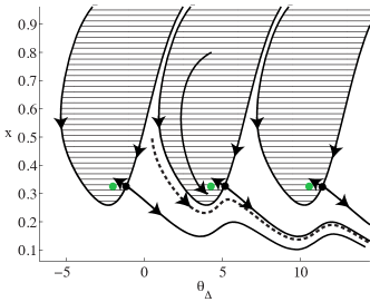
Figure 2: Phase portrait for $\omega_{\Delta}^{\text{free}}$ from the hold-in range. The system’s evolving state over time traces a trajectory $(x(t),\theta_{\Delta}(t))$. Trajectories can not intersect. Unstable equilibrium points, such as saddles — black dots, locally asymptotically stable equilibria — green dots, any of which has its own basin of attraction (shaded domain) bounded by stable saddle separatrices (black trajectories going to the saddles). There are initial states and corresponding trajectories (see, e.g. dashed trajectory), which are not attracted to an equilibrium.

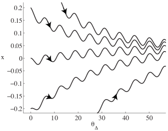
Figure 3: Phase portrait for $\omega_{\Delta}^{\text{free}}$ outside the hold-in range: there are no locally stable equilibria.

Thus, the equilibria can be considered as a multiple-valued function of variable $\omega_{\Delta}^{\text{free}}$: $\big{(}x_{eq}(\omega_{\Delta}^{\text{free}}),\theta_{eq}(\omega_{\Delta}^{\text{free}})\big{)}$. From the boundedness of the PD characteristic $\varphi(\theta_{eq})$ it follows that there are no equilibria for sufficiently large $|\omega_{\Delta}^{\text{free}}|$ (see Figs. 2 and 3).

IV Engineering definitions of stability ranges

The widely used engineering assumption (see Viterbi’s pioneering writing [4, p.15]) is that the zero input response of filter $\alpha_{0}(t,x_{0})$ does not affect the synchronization of the loop. This assumption allows the filter state $x(t)$ to be excluded from the consideration and a simplified mathematical model of PLL-based circuit in the signal’s phase space to be obtained from (4) and (5) (see, e.g. [4, p.17, eq.2.20] for $h=0$ and [3, p.41, eq.4-26] for $\gamma\equiv 0$):

$$\dot{\theta}_{\Delta}\!=\!\omega_{\Delta}^{\text{free}}-L\!\!\!\int_{0}^{t}\!\!\!\!\!\gamma(t-\tau)\varphi(\theta_{\Delta}(\tau)){\rm d}\tau-Lh\varphi(\theta_{\Delta}(t)).$$ (12)

For an example of this one-dimensional integro-differential equation the following intervals (​​[3, 4]) are defined: the hold-in range includes $|\omega_{\Delta}^{\text{free}}|$ such that model (12) has an equilibrium $\theta_{\Delta}(t)\equiv\theta_{eq}$, which is locally stable (local stability, i.e. for some initial phase error $\theta_{\Delta}(0)$); the pull-in range includes $|\omega_{\Delta}^{\text{free}}|$ such that any solution of model (12) is attracted to one of the equilibria $\theta_{eq}$ (global stability, i.e. for any initial phase error $\theta_{\Delta}(0)$). Thus, the block diagram of the loop in Fig. 1 is usually considered without initial data $x(0)$ and $\theta_{\Delta}(0)$ (see, e.g. [4, p.17, fig.2.3]).

Viterbi [4] explains the above assumption for the stable matrix $A$, but considers also various filters with marginally stable matrixes (e.g. a filter – perfect integrator, where $A=0$). At the same time, even for a stable matrix $A$, the initial filter state $x(0)$ and $\alpha_{0}(t,x_{0})$ may affect the acquisition process and stability ranges (see, e.g. corresponding examples for the classical PLL [20] and Costas loops [22, 23, 24, 21]).

While the above assumption allows introduction of the above one-dimensional stability sets, defined only by $|\omega_{\Delta}^{\text{free}}|$, for rigorous study the multi-dimensional stability domains have to considered, taking into account $x(0)$, and their relationships with the classical engineering ranges have to be explained. In [6, p.187] it is noted that the consideration of all state variables is of utmost importance in the study of cycle slips and the lock-in concept.

V Rigorous definitions of stability sets

The rigorous mathematical definitions of the hold-in, pull-in, and lock-in sets are now given for the nonlinear mathematical model of PLL-based circuits in the signal’s phase space (8) and corresponding nontrivial examples are considered.

V-A Local stability and hold-in set

We now consider the linearization of system (8) along an equilibrium $(x_{eq},\theta_{eq})$. Taking into account (11) and $\varphi^{\prime}(\theta):=d\varphi(\theta)/d\theta$, the linearized system is as follows:

$$\left(\begin{array}[]{c}\dot{x}\\ \dot{\theta}_{\Delta}\\ \end{array}\right)=\left(\begin{array}[]{cc}A&b\varphi^{\prime}(\theta_{eq})\\ -Lc^{*}&-Lh\varphi^{\prime}(\theta_{eq})\end{array}\right)\left(\begin{array}[]{c}x-x_{eq}\\ \theta_{\Delta}-\theta_{eq}\\ \end{array}\right)$$ (13)

The characteristic polynomial of linear system (8) can be written (using the Schur complement, e.g. [11]) in the following form: $\chi(s)=\big{(}-Lh\varphi^{\prime}(\theta_{eq})-s+Lc^{*}(A-sI)^{-1}b\varphi^{\prime}(\theta_{eq})\big{)}\det(A-sI)$, or can be expressed in terms of the filter’s transfer function $H(s)=\frac{a(s)}{d(s)}$, where $a(s)$ and $d(s)$ are polynomials:

$$\chi(s)=-\big{(}sd(s)+a(s)L\varphi^{\prime}(\theta_{eq})\big{)}.$$ (14)

The characteristic polynomial corresponds to the denominator of the closed loop transfer function.

To study the local stability of equilibria (11), it is necessary to check whether all the roots of the characteristic polynomial (14) for the linearization of model (8) along the equilibria (i.e. the poles of the closed loop transfer function) have negative real parts. For this purpose, at the stage of pre-design analysis when all parameters of the loop can be chosen precisely, the Routh-Hurwitz criterion and its analogs (see, e.g. Kharitonov’s generalization [30] for interval polynomials) can be effectively applied. At the stage of post-design analysis when only the input and VCO output are considered and the parameters are known only approximately, various frequency characteristics of the loop (see, e.g. Nyquist and Bode plots) and the continuation principle can be used (see, e.g, [6, 7]).

If the PD characteristic is an odd function and hence $\varphi^{\prime}(\theta_{eq})$ is an even function, from (9) we conclude that

1) there are symmetric equilibria: $\big{(}x_{eq}(\omega_{\Delta}^{\text{free}}),\theta_{eq}(\omega_{\Delta}^{\text{free}})\big{)}=\big{(}-x_{eq}(-\omega_{\Delta}^{\text{free}}),-\theta_{eq}(-\omega_{\Delta}^{\text{free}})\big{)}$,

2) these symmetric equilibria are simultaneously stable or unstable.

The same holds true for nonstationary trajectories.

Definition 1.

A set of all frequency deviations $|\omega_{\Delta}^{\text{free}}|$ such that the mathematical model of the loop in the signal’s phase space has a locally asymptotically stable equilibrium is called a hold-in set $\Omega_{\text{hold-in}}$.

Thus, a value of frequency deviation belongs to the hold-in set if the loop re-achieves locked state after small perturbations of the filter’s state, the phases and frequencies of VCO and the input signals. This effect is also called steady-state stability. In addition, for a frequency deviation within the hold-in set,

the loop in a locked state tracks small changes in input frequency, i.e. achieves a new locked state (tracking process).

In the literature the following explanations of the hold-in range (sometimes also called a lock range [31, p.507], [32, p.10-2], a synchronization range [33], a tracking range [1, p.49]) can be found: “The hold-in range is obtained by calculating the frequency where the phase error is at its maximum”[34, p.171], “The maximum frequency difference before losing lock of the PLL system is called the hold-in range”[8, p.258]. The following example shows that these explanations may not be correct, because for high-order filters the hold-in “range” may have holes.

The following example shows that the hold-in set may not include $\omega_{\Delta}^{\text{free}}=0$.

Example 1 (the hold-in set does not contain $\omega_{\Delta}^{\text{free}}=0$).

Consider the classical PLL with the sinusoidal PD characteristic $\varphi(\theta_{\Delta})=\frac{1}{2}\sin(\theta_{\Delta})$, VCO input gain $L=8$, and the filter transfer function

$$H(s)=\frac{a(s)}{d(s)}=\frac{1+0.5s}{1+0.5s+0.5s^{2}}.$$ (15)

From (11) the following equation for equilibria is obtained:

$$\frac{1}{2}\sin(\theta_{eq})=\frac{1}{8}\omega_{\Delta}^{\text{free}}.$$ (16)

Applying the Routh-Hurwitz stability criterion to the denominator of the closed loop transfer function (14)

$$s^{3}+s^{2}+s(2+4\cos(\theta_{eq}))+8\cos(\theta_{eq}),$$ (17)

the following conditions are obtained:

$$\cos(\theta_{eq})>0,\ (2+4\cos(\theta_{eq}))>0,$$ (18)

$$(2+4\cos(\theta_{eq}))>8\cos(\theta_{eq}).$$

Then $0<\cos(\theta_{eq})<\frac{1}{2}$, and for the locked state the steady-state phase error (i.e. corresponding to an equilibrium) is obtained

$$\theta_{eq}\in(-\frac{\pi}{2},-\frac{\pi}{3})\cup(\frac{\pi}{3},\frac{\pi}{2}).$$ (19)

Taking into account (16), (19), one obtains the hold-in set

$$|\omega_{\Delta}^{\text{free}}|\in(2\sqrt{3},4).$$ (20)

The next example shows that the hold-in set may not actually be a range (i.e., an interval) but a union of intervals, one of which may include $\omega_{\Delta}^{\text{free}}=0$.

Example 2 (the hold-in set is a union of disjoint intervals, one of which contains $\omega_{\Delta}^{\text{free}}=0$).

Consider the classical PLL with the sinusoidal PD characteristic $\varphi(\theta_{\Delta})=\frac{1}{2}\sin(\theta_{\Delta})$, the VCO input gain $L=80$, and the filter transfer function

$$H(s)=\frac{1+0.25s+0.5s^{2}}{1+2s+2s^{2}+2s^{3}}.$$ (21)

From (11) the following equation for the equilibria is obtained:

$$\frac{1}{2}\sin(\theta_{eq})=\frac{1}{80}\omega_{\Delta}^{\text{free}}.$$ (22)

An equilibrium is asymptotically stable if and only if all the roots of polynomial (14):

$$s(1+2s+2s^{2}+2s^{3})+K(1+0.25s+0.5s^{2})=$$ (23)

$$2s^{4}+2s^{3}+s^{2}(2+0.5K)+s(1+0.25K)+K,$$

$$K=L\varphi^{\prime}(\theta_{eq})=40\cos(\theta_{eq})$$

have negative real parts. Using the Routh-Hurwitz criterion, we obtain

$$2+0.5K>0,\ 1+0.25K>0,\ K>0,$$ (24)

$$2(2+0.5K)>2(1+0.25K),$$

$$2(2+0.5K)(1+0.25K)>2(1+0.25K)^{2}+2^{2}K.$$

From these inequalities we have

$$K=40\cos(\theta_{eq})\in(0,12-8\sqrt{2})\cup(12+8\sqrt{2},\infty),$$ (25)

$$\theta_{eq}\in(-\frac{\pi}{2},-1.5536)\cup(-0.9486,0.9486)\cup(1.5536,\frac{\pi}{2}).$$

Note that for other values of $\theta_{eq}$ at least one root of the polynomial (23) has a positive real part, making the corresponding equilibrium unstable. Combining (22) and (25), we obtain the hold-in set

$$|\omega_{\Delta}^{\text{free}}|\in[0,32.5)\cup(39.9942,40).$$ (26)

Note that in this case, for the values of the VCO input gain $L>24+16\sqrt{2}$ the hold-in set is always a union of disjoint intervals. For $L=80$ the simulation results of transition process in Simulink model  in Fig. 4 are shown in Figs. 5–7 for the initial data $(x(0)=(0;0;0.9990),\theta_{\Delta}(0)=1.5585)$ and various $\omega_{\Delta}^{\text{free}}$.

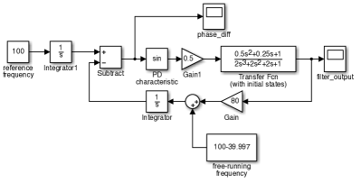
Figure 4: MatLab Simulink: the signal’s phase space model of the classical PLL

Related discussion on the frequency responses of loop with high-order filters can be found in [6, p.34-38, 52-56].

Remark 1.

For the first order filters, the set $\Omega_{\text{hold-in}}$ is an interval $|\omega_{\Delta}^{\text{free}}|<\omega_{h}$. For higher order filters, the set $\Omega_{\text{hold-in}}$ may be more complex. Thus, from an engineering point of view, it is reasonable to require that $\omega_{\Delta}^{\text{free}}=0$ belongs to the hold-in set and to define a hold-in range as the largest interval $[0,\omega_{h})$ from the hold-in set

$$[0,\omega_{h})\subset\Omega_{\text{hold-in}}$$

such that a certain stable equilibrium varies continuously when $\omega_{\Delta}^{\text{free}}$ is changed within the range. Here $\omega_{h}$ is called a hold-in frequency (see [3, p.38]).

Remark 2.

In the general case when there is no symmetry with respect to $\omega_{\Delta}^{\text{free}}$ (see (9)) the hold-in set need not be symmetric and the set $\omega_{\Delta}^{\text{free}}\in\Omega_{\text{hold-in}}$ must be considered in Definition 1.

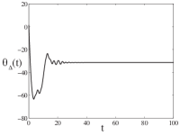
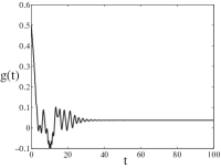
Figure 5: $\omega_{\Delta}^{\text{free}}=3$: stable locked state exists.

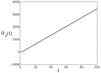
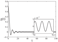
Figure 6: $\omega_{\Delta}^{\text{free}}=35$: there are no locked states (see also Fig. 3).

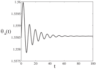
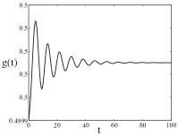
Figure 7: $\omega_{\Delta}^{\text{free}}=39.997$: stable locked state exists.

V-B Global stability (stability in the large) and pull-in set

Assume that the loop power supply is initially switched off and then at $t=0$ the power is switched on, and assume that the initial frequency difference is sufficiently large. The loop may not lock within one beat note, but the VCO frequency will be slowly tuned toward the reference frequency (acquisition process). This effect is also called a transient stability. The pull-in range is used to name such frequency deviations that make the acquisition process possible (see, e.g. explanations in [3, p.40], [7, p.61]).

To define a pull-in range (called also a capture range [41], an acquisition range [33, p.253]) rigorously, consider first an important definition from stability theory.

Definition 2.

If for a certain $\omega_{\Delta}^{\text{free}}$ any trajectory of system (8) tends to an equilibrium, then the system with such $\omega_{\Delta}^{\text{free}}$ is called globally asymptotically stable (see Fig. 8).

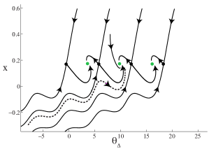
Figure 8: Phase portrait for $\omega_{\Delta}^{\text{free}}$ from the pull-in range: any trajectory is attracted to an equilibrium (equilibria: green–stable and black–unstable circles); for a sufficiently large initial state of the filter, cycle slipping is possible (see, e.g. dashed trajectory).

We now consider a possible rigorous definition.

Definition 3.

A set of all frequency deviations $|\omega_{\Delta}^{\text{free}}|$ such that the mathematical model of the loop in the signal’s phase space is globally asymptotically stable is called a pull-in set $\Omega_{\text{pull-in}}$.

Remark 3.

In the general case when there is no symmetry with respect to $\omega_{\Delta}^{\text{free}}$ the set $\omega_{\Delta}^{\text{free}}\in\Omega_{\text{pull-in}}$ has to be considered in Definition 3.

Remark 4.

The pull-in set is a subset of the hold-in set: $\Omega_{\text{pull-in}}\subset\Omega_{\text{hold-in}}$, and need not be an interval. From an engineering point of view, it is reasonable to require that $\omega_{\Delta}^{\text{free}}=0$ belongs to the pull-in set and to define a pull-in range as the largest interval $[0,\omega_{p})$ from the pull-in set:

$$[0,\omega_{p})\subset\Omega_{\text{pull-in}},$$

where $\omega_{p}$ is called a pull-in frequency (see [3, p.40]).

Remark 5.

If all possible states of the filter are bounded:

$$x\in X_{\text{real}}\ (\text{e.g.\ }X_{\text{real}}=\{x:c_{\text{min}}<|x|<c_{\text{max}}\}),$$

by the design of the circuit (e.g. capacitors have limited maximum and minimum charges, the VCO frequency is limited etc.), then in the definition of pull-in set it is reasonable to require that only solutions with $x(0)\in X_{\text{real}}$ tend to the stationary set. Trajectories, with initial data outside of the domain defined by $x(0)\in X_{\text{real}}$ (here the initial phase error $\theta_{\Delta}(0)$ can take any value), need not tend to the stationary set.

For the model without filter (i.e. $H(s)=const$) the pull-in set coincides with the hold-in set. The pull-in set of PLL-based circuits with first-order filters can be estimated using phase plane analysis methods [42, 43], but in general its rigorous study is a challenging task [4, 44, 12, 17, 45].

For the case of the passive lead-lag filter $H(s)=\frac{1+s\tau_{2}}{1+s(\tau_{1}+\tau_{2})}$, a recent work [12, p.123] notes that “the determination of the width of the capture range together with the interpretation of the capture effect in the second order type-I loops have always been an attractive theoretical problem. This problem has not yet been provided with a satisfactory solution”. At the same time in [46, 47, 48, 11] it is shown that the basin of attraction of the stationary set may be bounded (e.g. by a semistable periodic trajectory, which may appear as the result of collision of unstable and stable periodic solutions), and corresponding analytical estimations and bifurcation diagram are given.

Note that in this case a numerical simulation may give wrong estimates and should be used very carefully. For example, in [40] the SIMetrics SPICE model for a two-phase PLL with a lead-lag filter gives two essentially different results of simulation with default “auto” sampling step (acquires lock) and minimum sampling step set to $1m$ (does not acquire lock — such behaviour agrees with the theoretical analysis). The same problems are also observed in MatLab Simulink [49, 20, 21], see, e.g. Fig. 9. These examples demonstrate the difficulties of numerical search of so-called hidden oscillations [48, 50, 51], whose basin of attraction does not overlap with the neighborhood of an equilibrium point, and thus may be difficult to find numerically. In this case the observation of one or another stable solution may depend on the initial data and integration step.

Figure 9: Simulation of two-phase PLL described by Fig. 4 or model (8) [40]: $\tau_{1}\!=\!0.0448$, $\tau_{2}\!=\!0.0185$, $A\!=\!-\frac{1}{\tau_{1}+\tau_{2}}$, $b\!=\!1-\frac{\tau_{2}}{\tau_{1}+\tau_{2}}$, $c\!=\!\frac{1}{\tau_{1}+\tau_{2}}$, $h\!=\!\frac{\tau_{2}}{\tau_{1}+\tau_{2}}$; $\varphi(\theta_{\Delta})=\frac{1}{2}\sin(\theta_{\Delta})$; $\omega_{1}\!=\!10000$, $\omega_{2}^{\text{free}}\!=\!10000-178.9$, $L\!=\!500$. Filter output $g(t)$ for the initial data $x_{0}\!=\!0.1318,\theta_{\Delta}(0)\!=\!0$ obtained for default “auto” relative tolerance (red) — acquires lock, relative tolerance set to “1e-3”(green) — does not acquire lock.

S. Goldman, who has worked at Texas Instruments over 20 years, notes that PLLs are used as pipe cleaners for breaking simulation tools [54, p.XIII].

While PLL-based circuits are nonlinear control systems and for their nonlocal analysis it is essential to apply the classical stability criteria, which are developed in control theory, however their direct application to analysis of the PLL-based models is often impossible, because such criteria are usually not adapted for the cylindrical phase space; in the tutorial Phase Locked Loops: a Control Centric Tutorial [14], presented at the American Control Conference 2002, it was said that “The general theory of PLLs and ideas on how to make them even more useful seems to cross into the controls literature only rarely”.

At the same time the corresponding modifications of classical stability criteria for the nonlinear analysis of control systems in cylindrical phase space were well developed in the second half of the 20th century, see, e.g. [29, 58, 59, 60]. A comprehensive discussion and the current state of the art can be found in [11]. One reason why these works have remained almost unnoticed by the contemporary engineering community may be that they were written in the language of control theory and the theory of dynamical systems, and, thus, may not be well adapted to the terms and objects used in the engineering practice of phase-locked loops. Another possible reason, as noted in [61, p.1], is that the nonlinear analysis techniques are well beyond the scope of most undergraduate courses in communication theory and circuits design. Note that for the application of various stability criteria it is often necessary to represent system (8) in the Lur’e form:

$$\begin{aligned} \left(\!\!\!\begin{array}[]{c}\dot{\bar{x}}\\ \dot{\theta}_{\Delta}\\ \end{array}\!\!\!\right)=\left(\!\!\!\begin{array}[]{cc}A&0\\ -Lc^{*}&0\\ \end{array}\!\!\!\right)\left(\!\!\!\begin{array}[]{c}\bar{x}\\ \theta_{\Delta}\\ \end{array}\!\!\!\right)+\left(\!\!\!\begin{array}[]{c}b\\ -Lh\\ \end{array}\!\!\!\right)\bar{\varphi}(\theta_{\Delta})\end{aligned},$$ (27)

where

$$\bar{x}=x-x_{eq}=x+A^{-1}b\varphi(\theta_{eq}),\ \bar{\varphi}(\theta_{\Delta})=\varphi(\theta_{\Delta})-\varphi(\theta_{eq}),$$

$$\varphi(\theta_{eq})=\omega_{\Delta}^{\text{free}}L^{-1}(-c^{*}A^{-1}b+h)^{-1}.$$

See also discussion of some nonlinear methods for the analysis of PLL-based models in recent books [62, 12, 17, 13].

V-C Cycle slips and lock-in range

Let us rigorously define cycle slipping in the phase space of system (8).

Definition 4.

If

$$\limsup\limits_{t\to+\infty}|\theta_{\Delta}(0)-\theta_{\Delta}(t)|>2\pi,$$ (28)

it is then said that cycle slipping occurs (see, e.g. dashed trajectory in Fig. 8).

Here, sometimes, instead of the limit of the difference, the maximum of the difference is considered (see, e.g. [44, p.131]).

Definition 4’ If

$$\sup\limits_{t>0}|\theta_{\Delta}(0)-\theta_{\Delta}(t)|>2\pi,$$ (29)

it is then said that cycle slipping has occurred.

Note that, in general, Definition 4’ need not mean that finally (after acquisition) condition (28) can not be fulfilled.

Sometimes, the number of cycle slips is of interest.

Definition 5.

If

$$2k\pi<\limsup\limits_{t\to\infty}|\theta_{\Delta}(0)-\theta_{\Delta}(t)|<2(k+1)\pi,$$ (30)

it is then said that $k$ cycle slips occurred.

A numerical study of cycle slipping in classical PLL can be found in [63]. Analytical tools for estimating the number of cycle slips depending on the parameters of the loop can be found, e.g. in [64, 58, 11].

The concepts of lock-in frequency and lock-in range (called also a lock range[65, p.256], a seize range [66, p.138]), were intended to describe the set of frequency deviations for which the loop can acquire lock within one beat without cycle slipping. In [3, p.40] the following definition was introduced: “If, for some reason, the frequency difference between input and VCO is less than the loop bandwidth, the loop will lock up almost instantaneously without slipping cycles. The maximum frequency difference for which this fast acquisition is possible is called the lock-in frequency”.

However, in general, even for zero frequency deviation ($\omega_{\Delta}^{\text{free}}=0$) and a sufficiently large initial state of filter ($x(0)$), cycle slipping may take place (see, e.g. dashed trajectory in Fig. 10, left). Thus, considering of all state variables is of utmost importance for the cycle slip analysis and, therefore, the concept lock-in frequency lacks rigor for classical simplified model (12) because it does not take into account the initial state of the filter. The above definition of the lock-in frequency and corresponding definition of the lock-in range were subsequently in various engineering publications (see, e.g. [67, p.34-35],[68, p.161],[69, p.612],[70, p.532],[71, p.25], [1, p.49],[14, p.4],[72, p.24],[73, p.749],[74, p.56], [54, p.112],[7, p.61],[66, p.138],[75, p.576],[8, p.258]).

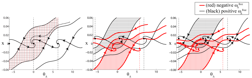
Figure 10: Phase portraits for the classical PLL with the following parameters: $H(s)=\frac{1+s\tau_{2}}{1+s(\tau_{1}+\tau_{2})}$, $\tau_{1}=4.48\cdot 10^{-2}$, $\tau_{2}=1.85\cdot 10^{-2}$, $L=250$, $\varphi(\theta_{\Delta})=\frac{1}{2}\sin(\theta_{\Delta})$, and various frequency deviations. Black color is for the system with positive $\omega_{\Delta}^{\text{free}}=|\widetilde{\omega}|$. Red is for the system with negative $\omega_{\Delta}^{\text{free}}=-|\widetilde{\omega}|$. Equilibria (dots), separatrices pass in and out of the saddles, local lock-in domains are shaded (upper black horizontal lines is for $\omega_{\Delta}^{\text{free}}>0$, lower red vertical lines is for $\omega_{\Delta}^{\text{free}}<0$). Left subfig: $\omega_{\Delta}^{\text{free}}=0$; middle subfig: $\omega_{\Delta}^{\text{free}}=\pm 65$; right subfig: $\omega_{\Delta}^{\text{free}}=\pm 68$.

.

The loop model (8) has a subdomain of the phase space, where trajectories do not slip cycles (called a lock-in domain), for each value of $\omega_{\Delta}^{\text{free}}$. The lock-in domain is the union of local lock-in domains, each of which corresponds to one of the equilibria and has its own shape (see, e.g. shaded domain in Fig. 10, left defined by corresponding separatrices). The shape of the lock-in domain significantly varies depending on $\omega_{\Delta}^{\text{free}}$. In [4, p.50]) a lock-in domain is called a frequency lock. Some writers (e.g. [44, p.132],[76, p.355]) use the concept lock-in range to denote a lock-in domain.

In general, taking into account nonuniform behavior of the lock-in domain shape, Gardner wrote “There is no natural way to define exactly any unique lock-in frequency” [9, p.70], [6, p.188].

Below we demonstrate how to overcome these problems and rigorously define a unique lock-in frequency and range.

We now consider a specific $\omega_{\Delta}^{\text{free}}$ and denote by $D_{\text{lock-in}}(\omega_{\Delta}^{\text{free}})$ the corresponding lock-in domain. Such a domain exists for any $|\omega_{\Delta}^{\text{free}}|\in\Omega_{\text{hold-in}}$ because at least the equilibria are contained in this domain. For a set $\omega_{\Delta}^{\text{free}}\in\Omega$ we consider the intersection of corresponding lock-in domains (see, e.g. the intersections of local lock-in domains for various $\omega_{\Delta}^{\text{free}}=\pm|\widetilde{\omega}|$ in Fig. 10 — domains shaded both by red vertical and black horizontal lines):

$${\rm D}_{\text{lock-in}}(\Omega)=\bigcap\limits_{\omega_{\Delta}^{\text{free}}\in\Omega}{\rm D}_{\text{lock-in}}(\omega_{\Delta}^{\text{free}}).$$

Definition 6.

A lock-in range is the largest interval $[0,\omega_{l})$ such that for any $|\omega_{\Delta}^{\text{free}}|\in[0,\omega_{l})$ the mathematical model of the loop in the signal’s phase space is globally asymptotically stable (i.e. $[0,\omega_{l})\subset[0,\omega_{p})$) and the following domain

$${\rm D}_{\text{lock-in}}\big{(}(-\omega_{l},\omega_{l})\big{)}=\bigcap\limits_{|\omega_{\Delta}^{\text{free}}|<\omega_{l}}{\rm D}_{\text{lock-in}}(\omega_{\Delta}^{\text{free}}).$$

contains all corresponding equilibria:

$$\big{(}x_{eq}(\omega_{\Delta}^{\text{free}}),\theta_{eq}(\omega_{\Delta}^{\text{free}})\big{)}\in{\rm D}_{\text{lock-in}}\big{(}(-\omega_{l},\omega_{l})\big{)}.$$

We call such domain ${\rm D}_{\text{lock-in}}={\rm D}_{\text{lock-in}}\big{(}(-\omega_{l},\omega_{l})\big{)}$ a uniform lock-in domain (uniform with respect to $(-\omega_{l},\omega_{l})$), $\omega_{l}$ is called a lock-in frequency (see [3, p.40]).

Various additional requirements may be imposed on the shape of the uniform lock-in domain ${\rm D}_{\text{lock-in}}$, e.g. it has to contain the line defined by $x\equiv 0$ (see, e.g. [8, p.258]) or the band defined by $|x|<c_{\text{max}}$. If instead of global stability in the definition of the pull-in set we consider stability in the domain defined by $X_{\text{real}}$, then we require that the intersection ${\rm D}_{\text{lock-in}}\bigcap X_{\text{real}}$ contains all corresponding equilibria.

Remark 6.

In the general case when there is no symmetry with respect to $\omega_{\Delta}^{\text{free}}$ we have to consider a unsymmetrical interval containing zero in Definition 6.

Similarly, we can define an extension of the lock-in range: $\Omega_{\text{lock-in}}\supset[0,\omega_{l})$, called a lock-in set (however, in general, such an extension may be not unique).

In other words, the definition implies that if the loop is in a locked state, then after an abrupt change of $\omega_{\Delta}^{\text{free}}$ within a lock-in range $[0,\omega_{l})$, the corresponding acquisition process in the loop leads, if it is not interrupted, to a new locked state without cycle slipping.

Finally, our definitions give $\Omega_{\text{lock-in}}\subset\Omega_{\text{pull-in}}\subset\Omega_{\text{hold-in}}.$ If there is a certain stable equilibrium varies continuously when $\omega_{\Delta}^{\text{free}}$ is changed within the hold-in, pull-in, and lock-in ranges (see Footnote 10), then

$$[0,\omega_{l})\subset[0,\omega_{p})\subset[0,\omega_{h})$$

which is in agreement with the classical consideration (see, e.g. [67, p.34],[69, p.612],[7, p.61],[66, p.138],[8, p.258]).

V-D Approximations of the lock-in range of the classical PLL

For the case of the classical odd PD characteristic (see Fig. 10), taking into account that equilibria are proportional to the frequency deviation (see (11)) and using the symmetry $\big{(}x_{eq}(\omega_{l}),\theta_{eq}(\omega_{l})\big{)}=-\big{(}x_{eq}(-\omega_{l}),\theta_{eq}(-\omega_{l})\big{)}$, we can effectively determine $\omega_{l}$. For that, we have to increase the frequency deviation $|\omega_{\Delta}^{\text{free}}|$ step by step and at each step, after the loop achieves a locked state, to change $\omega_{\Delta}^{\text{free}}=\widetilde{\omega}$ abruptly to $\omega_{\Delta}^{\text{free}}=-\widetilde{\omega}$ and to check if the loop can achieve a new locked state without cycle slipping. If so, then the considered value $|\omega_{\Delta}^{\text{free}}|$ belongs to $\Omega_{\text{lock-in}}$. If $\omega_{\Delta}^{\text{free}}\!=\!0$ belongs to $\Omega_{\text{pull-in}}$, then it is clear that $0$ belongs to $\Omega_{\text{lock-in}}$ (see Fig. 10, left). The limit value $\omega_{l}$ is defined by the case in Fig. 10, middle. At the next step when a value $|\omega_{\Delta}^{\text{free}}|=|\widetilde{\omega}|>\omega_{l}$ is considered, for $\omega_{\Delta}^{\text{free}}=-|\widetilde{\omega}|$ the
trajectory from the initial point, corresponding to a stable equilibrium for $\omega_{\Delta}^{\text{free}}\!=\!|\widetilde{\omega}|$ (see Fig. 10, right: red trajectory outgoing from a black dot), is attracted to an equilibrium only after cycle slipping. In other words [77], for this case:

The lock-in range is a subset of the pull-in range such that for each corresponding frequency deviation the lock-in domain (i.e. a domain of the loop states, where fast acquisition without cycle slipping is possible) contains both symmetric locked states (i.e. locked states for

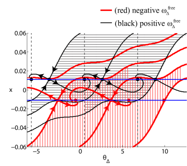
Figure 11: Phase portrait. Separatrices, equilibria and corresponding local lock-in domains (shaded): upper black is for $\omega_{\Delta}^{\text{free}}=61.5$, lower red is for $\omega_{\Delta}^{\text{free}}=-61,5$. The uniform lock-in domain is approximated by the band between two blue horizontal lines: $|x|\leq 0.0110$.

.

the positive and negative value of the difference between the reference frequency and the VCO free-running frequency).

In Fig. 10, middle the set ${\rm D}_{\text{lock-in}}$: contains all equilibria $x_{eq}(\omega_{\Delta}^{\text{free}})$ for $0\leq|\omega_{\Delta}^{\text{free}}|<\omega_{l}$. However for some non-equilibrium initial states from the band defined by $\{x:|x|<|x_{eq}(\omega_{l})|\}$ (phase error $\theta_{\Delta}$ takes all possible values), cycle slipping can take place. For example, see the points to the left and to the right of the black equilibrium states (i.e. for $\omega_{\Delta}^{\text{free}}=|\omega_{l}|>0$), lying above the red separatrix (i.e. for $\omega_{\Delta}^{\text{free}}=-|\omega_{l}|<0$), correspond to the red trajectories (i.e. for $\omega_{\Delta}^{\text{free}}=-|\omega_{l}|<0$), which are attracted to an equilibrium only after cycle slipping. To approximate the ${\rm D}_{\text{lock-in}}$ by a band, $\omega_{l}$ can be slightly decreased to cut the above points. In Fig. 11 the band defined by $X_{\text{lock-in}}=\{x:|x|<|x_{eq}(\widetilde{\omega}_{l})|,\ \widetilde{\omega}_{l}<\omega_{l}\}$ is contained in ${\rm D}_{\text{lock-in}}$ and for any initial state from the band the corresponding acquisition process in the loop leads, if it is not interrupted, to lock up without cycle slipping. Such a construction is more laborious and requires rigorous analysis of the phase space or exhaustive simulation.

Remark 7.

If we define (see, e.g. [78, p.92]) cycle slipping by the interval of maximum length $2\pi$ instead of $4\pi$ in Definition 4: i.e. $\limsup_{t\to\infty}|\theta_{\Delta}(0)-\theta_{\Delta}(t)|>\pi$, then for any $|\omega_{\Delta}^{\text{free}}|>0$ a distance between neighboring unstable and stable equilibria and a phase deviation of the corresponding unstable saddle separatrix may exceed $\pi$ (see, e.g. Fig. 11). Thus, the lock-in range may contain only $|\omega_{\Delta}^{\text{free}}|=0$.

Remark 8.

If the filter – perfect integrator can be implemented in considered architecture, the loop can be designed with the first order PI filter having the transfer function $H(s)=\frac{1+s\tau_{2}}{s\tau_{1}}$. Equations of the loop in this case become

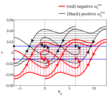
Figure 12: Phase portraits for the classical PLL with the following parameters: $H(s)=\frac{1+0.0225s}{0.0633s}$, $L=250$, and $\omega_{\Delta}^{\text{free}}=\pm 47$. Separatrices, equilibria and corresponding local lock-in domains (shaded): upper black is for $\omega_{\Delta}^{\text{free}}=47$, lower red is for $\omega_{\Delta}^{\text{free}}=-47$. The uniform lock-in domain is approximated by the band between the two blue horizontal lines: $|x|\leq 0.0119$.

$$\dot{x}=\frac{1}{\tau_{1}}\varphi(\theta_{\Delta}),\ \ \dot{\theta}_{\Delta}=\omega_{\Delta}^{\text{free}}-Lx-L\frac{\tau_{2}}{\tau_{1}}\varphi(\theta_{\Delta}),$$ (31)

or equivalently

$$\ddot{\theta}_{\Delta}=-L\frac{1}{\tau_{1}}\varphi(\theta_{\Delta})-L\frac{\tau_{2}}{\tau_{1}}\varphi^{\prime}(\theta_{\Delta})\dot{\theta}_{\Delta}.$$ (32)

Here the equilibria are defined from the equations

$$\varphi(\theta_{eq})=0,\ \ x_{eq}={\omega_{\Delta}^{\text{free}}L^{-1}}.$$

Because model (32) does not depend explicitly on $\omega_{\Delta}^{\text{free}}$, the hold-in and pull-in ranges are either infinite or empty. Note, that the parameter $\omega_{\Delta}^{\text{free}}$ shifts the phase plane vertically (in the variable $x$) without distorting trajectories, which simplifies the analysis of the uniform lock-in domain and range (see Fig. 12). If the transfer function $H(s)$ of a high order filter has the term $s^{r}$ with $r\in\mathbb{N}$ in the denominator, then instead of equilibria we have a stationary linear manifold: $\varphi(\theta_{eq})=0,\ c_{1}x_{eq}^{1}+\ldots+c_{r}x_{eq}^{r}=\frac{-\omega_{\Delta}^{\text{free}}}{L}.$

For the classical PLL with the filter’s transfer function $H(s)=\frac{\beta+\alpha s}{s}$ it can be analytically proved that the pull-in range is theoretically infinite. Some needed explanations are given by Viterbi [4] using phase plane analysis. But, even in such a simple case, rigorous phase plane analysis is a complex task (e.g. [79], the proof of the nonexistence of heteroclinic and first-order cycles is omitted in [4]). The rigorous analytical proof can be effectively achieved by considering a special Lyapunov function [55, 11, 79]: $V(x,\theta_{\Delta})=\frac{1}{2}\big{(}x-\frac{\omega_{\Delta}^{\text{free}}}{L}\big{)}^{2}+\frac{2\beta}{L}\sin^{2}{\frac{\theta_{\Delta}}{2}}\geq 0$ and $\dot{V}(x,\theta_{\Delta})=-h\beta\sin^{2}{\theta_{\Delta}}\leq 0$. Here it is important that for any $\omega_{\Delta}^{\text{free}}$ the set $\dot{V}(x,\theta_{\Delta})\equiv 0$ does not contain the whole trajectories of system (31) except for equilibria.

V-E Initial and free-running frequencies of VCO

Note that in the above Definitions 1, 3, and 6 the hold-in, pull-in, and lock-in sets are defined by the frequency deviation, i.e. by the absolute value of the difference between VCO free-running frequency (in the open loop) and the input signal’s frequency: $|\omega_{\Delta}^{\text{free}}|=|\omega_{1}-\omega_{2}^{\text{free}}|$. The VCO free-running frequency $\omega_{2}^{\text{free}}$ is different from the VCO initial frequency $\omega_{2}(0)$: $\omega_{2}(0)=\omega_{2}^{\text{free}}+g(0),$ where $g(0)=c^{*}x(0)+h\varphi(\theta_{\Delta}(0))$ is the initial control signal, depending on the initial states of the filter $x(0)$ and the initial phase difference $\theta_{\Delta}(0)$.

It is interesting that for simplified model (12) with $h=0$ (see eq. 2.20 in the classic reference [4]) the absolute value of the initial difference between frequencies $|\dot{\theta}_{\Delta}(0)|=|\omega_{\Delta}(0)|=|\omega_{1}-\omega_{2}(0)|$ is equal to the frequency deviation $|\omega_{\Delta}^{\text{free}}|=|\omega_{1}-\omega_{2}^{\text{free}}|$. Following such simplified consideration in engineering literature the concept of an “initial frequency difference” can be found to be in use instead of the concept of a “frequency deviation”: see, e.g. [3, p.44] “If the initial frequency difference (between VCO and input) is within the pull-in range, the VCO frequency will slowly change in a direction to reduce the difference”, [80, p.1792] “The maximum frequency difference between the input and the output that the PLL can lock within one single beat note is called the lock-in range of the PLL”, [1, p.49] “Whether the PLL can get synchronized at all or not depends on the initial frequency difference between the input signal and the output of the controlled oscillator.” In general, the change of $\omega_{2}^{\text{free}}$ to $\omega_{2}(0)$ may lead to wrong results in the above definitions of ranges because in the case of $x(0)\neq 0$, $h\neq 0$ or non-odd function $\varphi(\theta_{\Delta})$ for the same values of $\omega_{2}(0)$ the loop can achieve synchronization or not depending on the filter’s initial state $x(0)$, the initial phase difference $\theta_{\Delta}(0)$, and $\omega_{2}^{\text{free}}$. See the corresponding example.

Example 3.

Consider the behavior of model (8) for the sinusoidal signals (i.e. $\varphi(\theta_{\Delta})={1\over 2}\sin(2\theta_{\Delta})$) and the fixed parameters: $\omega_{\Delta}=100,H(s)=\frac{(1+s\tau_{2})}{1+s(\tau_{1}+\tau_{2})},\tau_{1}=0.0448,\tau_{2}=0.0185,L=250$. In Fig. 13 the phase portrait of system (8) is shown. The blue dash line consists of points for which the initial frequency difference is zero: $\omega_{\Delta}(0)=\dot{\theta}_{\Delta}(0)=0$. Despite the fact that the initial frequency differences of all trajectories outgoing from the blue line are the same (equal to $0$), the green trajectory tends to a locked state while the magenta trajectory can not achieve this.

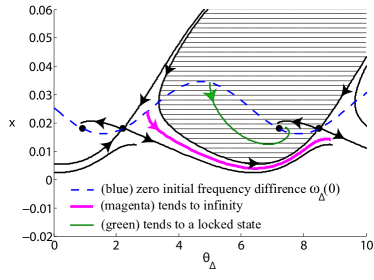
Figure 13: Phase portrait for $\omega_{\Delta}^{\text{free}}=100$. Blue dash curve corresponds to the set defined by $\dot{\theta}_{\Delta}(0)=0$. Initial points of the green (upper) and magenta (lower) trajectories correspond to the same initial frequency difference $\omega_{\Delta}(0)=0$.

VI CONCLUSIONS

This survey discussed a disorder and inconsistency in the definitions of ranges currently used. An attempt is made to discuss and fill some of the gaps identified between mathematical control theory, the theory of dynamical systems and the engineering practice of phase-locked loops. Rigorous mathematical definitions for the hold-in, pull-in, and lock-in ranges are suggested. The problem of unique lock-in frequency definition, posed by Gardner [9], is solved and an effective way to determine the unique lock-in frequency is suggested.

Gennady Leonov received his Candidate degree in 1971 and Dr.Sci. in 1983 from Saint-Petersburg State University. In 1986 he was awarded the USSR State Prize for development of the theory of phase synchronization for radiotechnics and communications. Since 1988 he has been Dean of the Faculty of Mathematics and Mechanics at Saint-Petersburg State University and since 2007 Head of the Department of Applied Cybernetics. He is member (corresponding) of the Russian Academy of Science, in 2011 he was elected to the IFAC Council. His research interests are now in control theory and dynamical systems.

Nikolay Kuznetsov received his Candidate degree from Saint-Petersburg State University (2004) and PhD from the University of Jyväskylä (2008). He is currently Deputy Head of the Department of Applied Cybernetics at Saint-Petersburg State University and Adjunct Professor at the University of Jyväskylä. His interests are now in dynamical systems stability and oscillations, Lyapunov exponent, chaos, hidden attractors, phase-locked loop nonlinear analysis, nonlinear control systems. E-mail: nkuznetsov239@gmail.com (corresponding author)

Marat Yuldashev received his Candidate degree from St.Petersburg State University (2013) and PhD from the University of Jyväskylä (2013). He is currently at Saint-Petersburg University. His research interests cover nonlinear models of phase-locked loops and Costas loops, and SPICE simulation.

Renat Yuldashev received his Candidate degree from St.Petersburg State University (2013) and PhD from the University of Jyväskylä (2013). He is currently at Saint-Petersburg University. His research interests cover nonlinear models of phase-locked loops and Costas loops, and simulation in MatLab Simulink.

References

- [1] M. Kihara, S. Ono, and P. Eskelinen, Digital Clocks for Synchronization and Communications. Artech House, 2002.
- [2] W. Lindsey and R. Tausworthe, A Bibliography of the Theory and Application of the Phase-lock Principle, ser. JPL technical report. Jet Propulsion Laboratory, California Institute of Technology, 1973.
- [3] F. Gardner, Phase-lock techniques. New York: John Wiley & Sons, 1966.
- [4] A. Viterbi, Principles of coherent communications. New York: McGraw-Hill, 1966.
- [5] V. Shakhgil’dyan and A. Lyakhovkin, Fazovaya avtopodstroika chastoty (in Russian). Moscow: Svyaz’, 1966.
- [6] F. Gardner, Phaselock Techniques, 3rd ed. Wiley, 2005.
- [7] R. Best, Phase-Lock Loops: Design, Simulation and Application, 6th ed. McGraw-Hill, 2007.
- [8] V. Kroupa, Frequency Stability: Introduction and Applications, ser. IEEE Series on Digital & Mobile Communication. Wiley-IEEE Press, 2012.
- [9] F. Gardner, Phase-lock techniques, 2nd ed. New York: John Wiley & Sons, 1979.
- [10] W. Davis, Radio Frequency Circuit Design, ser. Wiley Series in Microwave and Optical Engineering. Wiley, IEEE Press, 2011.
- [11] G. A. Leonov and N. V. Kuznetsov, Nonlinear Mathematical Models Of Phase-Locked Loops. Stability and Oscillations. Cambridge Scientific Press, 2014.
- [12] N. Margaris, Theory of the Non-Linear Analog Phase Locked Loop. New Jersey: Springer Verlag, 2004.
- [13] A. Suarez, Analysis and Design of Autonomous Microwave Circuits, ser. Wiley Series in Microwave and Optical Engineering. Wiley-IEEE Press, 2009.
- [14] D. Abramovitch, “Phase-locked loops: A control centric tutorial,” in American Control Conf. Proc., vol. 1. IEEE, 2002, pp. 1–15.
- [15] ——, “Method for guaranteeing stable non-linear PLLs,” 2004, US Patent App. 10/414,791, http://www.google.com/patents/US20040208274.
- [16] N. Krylov and N. Bogolyubov, Introduction to non-linear mechanics. Princeton: Princeton Univ. Press, 1947.
- [17] J. Kudrewicz and S. Wasowicz, Equations of phase-locked loop. Dynamics on circle, torus and cylinder. World Scientific, 2007.
- [18] G. A. Leonov, N. V. Kuznetsov, M. V. Yuldahsev, and R. V. Yuldashev, “Analytical method for computation of phase-detector characteristic,” IEEE Transactions on Circuits and Systems - II: Express Briefs, vol. 59, no. 10, pp. 633–647, 2012. 10.1109/TCSII.2012.2213362
- [19] G. A. Leonov, N. V. Kuznetsov, M. V. Yuldashev, and R. V. Yuldashev, “Nonlinear dynamical model of Costas loop and an approach to the analysis of its stability in the large,” Signal processing, vol. 108, pp. 124–135, 2015. 10.1016/j.sigpro.2014.08.033
- [20] N. Kuznetsov, O. Kuznetsova, G. Leonov, P. Neittaanmaki, M. Yuldashev, and R. Yuldashev, “Limitations of the classical phase-locked loop analysis,” in International Symposium on Circuits and Systems (ISCAS). IEEE, 2015, pp. 533–536, http://arxiv.org/pdf/1507.03468v1.pdf.
- [21] R. Best, N. Kuznetsov, O. Kuznetsova, G. Leonov, M. Yuldashev, and R. Yuldashev, “A short survey on nonlinear models of the classic Costas loop: rigorous derivation and limitations of the classic analysis,” in American Control Conference (ACC). IEEE, 2015, pp. 1296–1302, http://arxiv.org/pdf/1505.04288v1.pdf.
- [22] E. V. Kudryasoha, O. A. Kuznetsova, N. V. Kuznetsov, G. A. Leonov, S. M. Seledzhi, M. V. Yuldashev, and R. V. Yuldashev, “Nonlinear models of BPSK Costas loop,” ICINCO 2014 - Proceedings of the 11th International Conference on Informatics in Control, Automation and Robotics, vol. 1, pp. 704–710, 2014. 10.5220/0005050707040710
- [23] N. Kuznetsov, O. Kuznetsova, G. Leonov, P. Neittaanmaki, M. Yuldashev, and R. Yuldashev, “Simulation of nonlinear models of QPSK Costas loop in Matlab Simulink,” in 2014 6th International Congress on Ultra Modern Telecommunications and Control Systems and Workshops (ICUMT), vol. 2015-January. IEEE, 2014, pp. 66–71. 10.1109/ICUMT.2014.7002080
- [24] N. Kuznetsov, O. Kuznetsova, G. Leonov, S. Seledzhi, M. Yuldashev, and R. Yuldashev, “BPSK Costas loop: Simulation of nonlinear models in Matlab Simulink,” in 2014 6th International Congress on Ultra Modern Telecommunications and Control Systems and Workshops (ICUMT), vol. 2015-January. IEEE, 2014, pp. 83–87. 10.1109/ICUMT.2014.7002083
- [25] R. E. Best, N. V. Kuznetsov, G. A. Leonov, M. V. Yuldashev, and R. V. Yuldashev, “Simulation of analog Costas loop circuits,” International Journal of Automation and Computing, vol. 11, no. 6, pp. 571–579, 2014, 10.1007/s11633-014-0846-x.
- [26] M. Biggio, F. Bizzarri, A. Brambilla, and M. Storace, “Accurate and efficient PSD computation in mixed-signal circuits: a time domain approach,” Circuits and Systems II: Express Briefs, IEEE Transactions on, vol. 61, no. 11, 2014.
- [27] ——, “Efficient transient noise analysis of non-periodic mixed analogue/digital circuits,” IET Circuits, Devices & Systems, vol. 9, no. 2, pp. 73–80, 2015.
- [28] F. Bizzarri, A. Brambilla, and G. S. Gajani, “Periodic small signal analysis of a wide class of type-II phase locked loops through an exhaustive variational model,” Circuits and Systems I: Regular Papers, IEEE Transactions on, vol. 59, no. 10, pp. 2221–2231, 2012.
- [29] A. Gelig, G. Leonov, and V. Yakubovich, Stability of Nonlinear Systems with Nonunique Equilibrium (in Russian). Nauka, 1978, (English transl: Stability of Stationary Sets in Control Systems with Discontinuous Nonlinearities, 2004, World Scientific).
- [30] V. Kharitonov, “Asymptotic stability of an equilibrium position of a family of systems of differential equations,” Differentsialnye uravneniya, vol. 14, pp. 2086–2088, 1978.
- [31] D. Pederson and K. Mayaram, Analog Integrated Circuits for Communication: Principles, Simulation and Design. Springer, 2008.
- [32] U. Bakshi and A. Godse, Linear ICs and applications. Technical Publications, 2009.
- [33] A. Blanchard, Phase-Locked Loops. Wiley, 1976.
- [34] F. Brendel, Millimeter-Wave Radio-over-Fiber Links based on Mode-Locked Laser Diodes, ser. Karlsruher Forschungsberichte aus dem Institut für Hochfrequenztechnik und Elektronik. KIT Scientific Publishing, 2013.
- [35] S. Brigati, F. Francesconi, A. Malvasi, A. Pesucci, and M. Poletti, “Modeling of fractional-N division frequency synthesizers with SIMULINK and MATLAB,” in 8th IEEE International Conference on Electronics, Circuits and Systems, 2001. ICECS 2001, vol. 2, 2001, pp. 1081–1084 vol.2.
- [36] B. Nicolle, W. Tatinian, J.-J. Mayol, J. Oudinot, and G. Jacquemod, “Top-down PLL design methodology combining block diagram, behavioral, and transistor-level simulators,” in IEEE Radio Frequency Integrated Circuits (RFIC) Symposium,, 2007, pp. 475–478.
- [37] G. Zucchelli, “Phase locked loop tutorial,” http://www.mathworks.com/matlabcentral/fileexchange/14868-phase-locked-loop-tutorial, 2007.
- [38] H. Koivo and M. Elmusrati, Systems Engineering in Wireless Communications. Wiley, 2009.
- [39] R. Kaald, I. Lokken, B. Hernes, and T. Saether, “High-level continuous-time Sigma-Delta design in Matlab/Simulink,” in NORCHIP, 2009. IEEE, 2009, pp. 1–6.
- [40] G. Bianchi, N. Kuznetsov, G. Leonov, M. Yuldashev, and R. Yuldashev, “Limitations of PLL simulation: hidden oscillations in SPICE analysis,” arXiv:1506.02484, 2015, http://arxiv.org/pdf/1506.02484.pdf, http://www.mathworks.com/matlabcentral/fileexchange/52419-hidden-oscillations-in-pll (accepted to IEEE 7th International Congress on Ultra Modern Telecommunications and Control Systems).
- [41] D. Talbot, Frequency Acquisition Techniques for Phase Locked Loops. Wiley-IEEE Press, 2012.
- [42] F. Tricomi, “Integrazione di unequazione differenziale presentatasi in elettrotechnica,” Annali della R. Shcuola Normale Superiore di Pisa, vol. 2, no. 2, pp. 1–20, 1933.
- [43] A. A. Andronov, E. A. Vitt, and S. E. Khaikin, Theory of Oscillators (in Russian). ONTI NKTP SSSR, 1937, (English transl. 1966, Pergamon Press).
- [44] J. Stensby, Phase-Locked Loops: Theory and Applications, ser. Phase-locked Loops: Theory and Applications. Taylor & Francis, 1997.
- [45] R. Pinheiro and J. Piqueira, “Designing all-pole filters for high-frequency phase-locked loops,” Mathematical Problems in Engineering, vol. 2014, 2014, art. num. 682318.
- [46] B. Shakhtarin, “Study of a piecewise-linear system of phase-locked frequency control,” Radiotechnica and electronika (in Russian), no. 8, pp. 1415–1424, 1969.
- [47] L. Belyustina, V. Brykov, K. Kiveleva, and V. Shalfeev, “On the magnitude of the locking band of a phase-shift automatic frequency control system with a proportionally integrating filter,” Radiophysics and Quantum Electronics, vol. 13, no. 4, pp. 437–440, 1970.
- [48] G. A. Leonov and N. V. Kuznetsov, “Hidden attractors in dynamical systems. From hidden oscillations in Hilbert-Kolmogorov, Aizerman, and Kalman problems to hidden chaotic attractors in Chua circuits,” International Journal of Bifurcation and Chaos, vol. 23, no. 1, 2013, art. no. 1330002. 10.1142/S0218127413300024
- [49] N. Kuznetsov, G. Leonov, M. Yuldashev, and R. Yuldashev, “Nonlinear analysis of classical phase-locked loops in signal’s phase space,” IFAC Proceedings Volumes (IFAC-PapersOnline), vol. 19, pp. 8253–8258, 2014. 10.3182/20140824-6-ZA-1003.02772
- [50] N. Kuznetsov and G. Leonov, “Hidden attractors in dynamical systems: systems with no equilibria, multistability and coexisting attractors,” IFAC Proceedings Volumes (IFAC-PapersOnline), vol. 19, pp. 5445–5454, 2014. 10.3182/20140824-6-ZA-1003.02501
- [51] G. Leonov, N. Kuznetsov, and T. Mokaev, “Homoclinic orbits, and self-excited and hidden attractors in a Lorenz-like system describing convective fluid motion,” Eur. Phys. J. Special Topics, vol. 224, no. 8, pp. 1421–1458, 2015. 10.1140/epjst/e2015-02470-3
- [52] T. Lauvdal, R. Murray, and T. Fossen, “Stabilization of integrator chains in the presence of magnitude and rate saturations: a gain scheduling approach,” in Proc. IEEE Control and Decision Conference, vol. 4, 1997, pp. 4404–4005.
- [53] W. P. Heath, J. Carrasco, and M. de la Sen, “Second-order counterexamples to the discrete-time Kalman conjecture,” Automatica, vol. 60, pp. 140 – 144, 2015.
- [54] S. Goldman, Phase-Locked Loops Engineering Handbook for Integrated Circuits. Artech House, 2007.
- [55] Y. N. Bakaev, “Stability and dynamical properties of astatic frequency synchronization system,” Radiotekhnika i Elektronika, vol. 8, no. 3, pp. 513–516, 1963.
- [56] D. Abramovitch, “Lyapunov redesign of analog phase-lock loops,” Communications, IEEE Transactions on, vol. 38, no. 12, pp. 2197–2202, 1990.
- [57] ——, “Lyapunov redesign of classical digital phase-lock loops,” in American Control Conference, 2003. Proceedings of the 2003, vol. 3. IEEE, 2003, pp. 2401–2406.
- [58] G. A. Leonov, V. Reitmann, and V. B. Smirnova, Nonlocal Methods for Pendulum-like Feedback Systems. Stuttgart-Leipzig: Teubner Verlagsgesselschaft, 1992.
- [59] G. A. Leonov, D. V. Ponomarenko, and V. B. Smirnova, Frequency-Domain Methods for Nonlinear Analysis. Theory and Applications. Singapore: World Scientific, 1996.
- [60] G. A. Leonov, I. M. Burkin, and A. I. Shepelyavy, Frequency Methods in Oscillation Theory. Dordretch: Kluwer, 1996.
- [61] W. Tranter, T. Bose, and R. Thamvichai, Basic Simulation Models of Phase Tracking Devices Using MATLAB, ser. Synthesis lectures on communications. Morgan & Claypool, 2010.
- [62] A. Suarez and R. Quere, Stability Analysis of Nonlinear Microwave Circuits. Artech House, 2003.
- [63] G. Ascheid and H. Meyr, “Cycle slips in phase-locked loops: A tutorial survey,” Communications, IEEE Transactions on, vol. 30, no. 10, pp. 2228–2241, 1982.
- [64] O. B. Ershova and G. A. Leonov, “Frequency estimates of the number of cycle slidings in phase control systems,” Avtomat. Remove Control, vol. 44, no. 5, pp. 600–607, 1983.
- [65] K. Yeo, M. Do, and C. Boon, Design of CMOS RF Integrated Circuits and Systems. World Scientific, 2010.
- [66] W. Egan, Phase-Lock Basics. Wiley-IEEE Press, 2007.
- [67] R. Best, Phase-locked Loops: Design, Simulation, and Applications. McGraw Hill, 1984.
- [68] D. Wolaver, Phase-locked Loop Circuit Design. Prentice Hall, 1991.
- [69] G.-C. Hsieh and J. Hung, “Phase-locked loop techniques. A survey,” Industrial Electronics, IEEE Transactions on, vol. 43, no. 6, pp. 609–615, 1996.
- [70] J. Irwin, The Industrial Electronics Handbook. Taylor & Francis, 1997.
- [71] J. Craninckx and M. Steyaert, Wireless CMOS Frequency Synthesizer Design. Springer, 1998.
- [72] B. De Muer and M. Steyaert, CMOS Fractional-N Synthesizers: Design for High Spectral Purity and Monolithic Integration. Springer, 2003.
- [73] S. Dyer, Wiley Survey of Instrumentation and Measurement. Wiley, 2004.
- [74] K. Shu and E. Sanchez-Sinencio, CMOS PLL synthesizers: analysis and design. Springer, 2005.
- [75] R. Baker, CMOS: Circuit Design, Layout, and Simulation, ser. IEEE Press Series on Microelectronic Systems. Wiley-IEEE Press, 2011.
- [76] U. Meyer-Baese, Digital Signal Processing with Field Programmable Gate Arrays. Springer, 2004.
- [77] N. Kuznetsov, G. Leonov, M. Yuldashev, and R. Yuldashev, “Rigorous mathematical definitions of the hold-in and pull-in ranges for phase-locked loops,” in 1st IFAC Conference on Modelling, Identification and Control of Nonlinear Systems. IFAC Proceedings Volumes (IFAC-PapersOnline), 2015, pp. 720–723.
- [78] B. Purkayastha and K. Sarma, A Digital Phase Locked Loop based Signal and Symbol Recovery System for Wireless Channel. Springer, 2015.
- [79] K. Alexandrov, N. Kuznetsov, G. Leonov, P. Neittaanmaki, and S. Seledzhi, “Pull-in range of the pll-based circuits with proportionally-integrating filter,” in 1st IFAC Conference on Modelling, Identification and Control of Nonlinear Systems. IFAC Proceedings Volumes (IFAC-PapersOnline), 2015, pp. 730–734.
- [80] W. Chen, The Circuits and Filters Handbook, ser. Circuits & Filters Handbook. Taylor & Francis, 2002.