The color of smiling: computational synaesthesia of facial expressions

Abstract

This note gives a preliminary account of the transcoding or rechanneling problem between different stimuli as it is of interest for the natural interaction or affective computing fields. By the consideration of a simple example, namely the color response of an affective lamp to a sensed facial expression, we frame the problem within an information-theoretic perspective. A full justification in terms of the Information Bottleneck principle promotes a latent affective space, hitherto surmised as an appealing and intuitive solution, as a suitable mediator between the different stimuli.

1 Introduction

At the heart of non-verbal interaction between agents, either artificial or biological, is a rechannelling ability, namely the ability of gathering data from one kind of signal and instantaneously turn it into a different kind of signal. In artificial agents, such rechannelling or transcoding ability must be simulated through some form of “computational synaesthesia”. Strictly speaking, synaesthesia is a neurological phenomenon in which stimulation of one sensory or cognitive pathway leads to automatic, involuntary experiences in a second sensory or cognitive pathway [30]. Here, more liberally, we adopt it as a good metaphor for such rechannelling/transcoding of information [22].

In this note, as a case study, we consider the problem of transducing a sensed facial expression into a color stimuli. Denote $\mathbf{V}$ and $\mathbf{C}$ the random variables (RVs) standing for a visible expression display and for an emitted color stimulus, respectively. Then, the transcoding $\mathbf{V}\mapsto\mathbf{C}$ can be described in probabilistic terms as that of sampling a specific color stimulus $\mathbf{c}$, when expression stimulus $\mathbf{v}$ is observed, namely

$$\mathbf{c}\sim P(\mathbf{C}\mid\mathbf{V}=\mathbf{v}),$$ (1)

where $P(\mathbf{C}\mid\mathbf{V})$ is the conditional probability density function (pdf) defining the probability of generating a color stimulus $\mathbf{c}$ conditioned on the observation of expression $\mathbf{v}$. Such kind of problem is of interest for many applications in social signal processing [28], natural interaction [22], social robotics [14]. But, most important, here we discuss how a principled solution involves deep issues in spite of the apparent specificity of the problem.

An appealing way to conceive transcoding is through the mediation of some kind of latent space in particular a space of affective or emotional experience, which confers a unified semantics to the different kinds of non-verbal signals. It has been argued that this could be necessary for grounding synaesthetic cross-modal correspondences [24, 6], simulation-based theory of emotion and empathy [29]. Also, the mediation of a continuous dimensional space has been advocated for analyzing many different expressive modalities and to the purpose of building affective objects [22]. To such aim, we focus on the Pleasure/Arousal/Dominance space (PAD, [21]) as a continuous latent space to support “synesthesia” of facial expressions into color.

In this study we discuss how such solution can be conceived and grounded in an information-theoretic perspective, namely the Information Bottleneck (IB) framework introduced in [26] (cfr. Section 2).

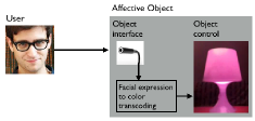
Figure 1: The Mood Lamp: an affective “synaesthetic” object that responds to user’s facial expressions by changing the color of the light emitted.

As a proof of concept we present the Mood Lamp (cfr. Fig. 1). The Mood Lamp is a kind of affective object, that is a “physical object which has the ability to sense emotional data from a person, map that information to an abstract form of expression and communicate that information expressively, either back to the subject herself or to another person”[22]. In particular, here a facial expression is used to convey affect states to an Ikea RGB color lamp, which will respond by changing the color of the light emitted in accordance with the affect.

Modeling computational synaesthesia as specified through Eq. 1 in the IB perspective has the advantage of providing a principled approach, characterized by a minimum of assumptions (Section 3). However there are a number of subtle difficulties to overcome that deserve being discussed (cfr. Sections 4 and 5).

2 Background and rationales

Central to this work is the idea that the synaesthetic transduction $\mathbf{V}\mapsto\mathbf{C}$ can be performed by resorting to an affect space, say $\mathbf{E}$, as a mediating factor.

Resorting to affect for transcoding stimuli may seem prima facie an instrumental approach; however, two issues bear on this choice. First, the insight of an affect space as a common factor for rechanneling between kinds of information is a not new in the psychological literature. On the one hand, perception and emotion are closely linked [18]. For instance, as to the specific case of synaesthetic cross-modal correspondences, affective similarity [24] has been suggested as a contributing factor: stimuli may be matched if they both happen to increase an observer’s level of alertness or arousal, or if they both happen to have the same effect on an observer’s emotional state, mood, or affective state. Efficient handling of affective synesthesia has been discussed by Collier who has shown [6] that both perceptual stimuli – such as colours, shapes, and musical fragments – and human emotions can be represented in a simple multidimensional space with two or three corresponding dimensions. Clearly this idea is consistent with the framework of an underpinning continuous “affect space”, which can be approximated by either two primary dimensions, e.g. valence and activity (arousal) [17], or three such as pleasure, arousal, and dominance (PAD) as proposed by Russell and Mehrabian [21] .

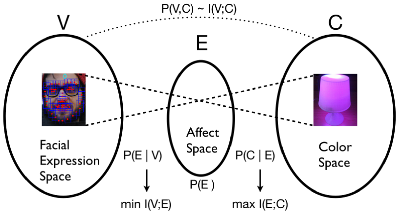
(a) (a) The IB framework

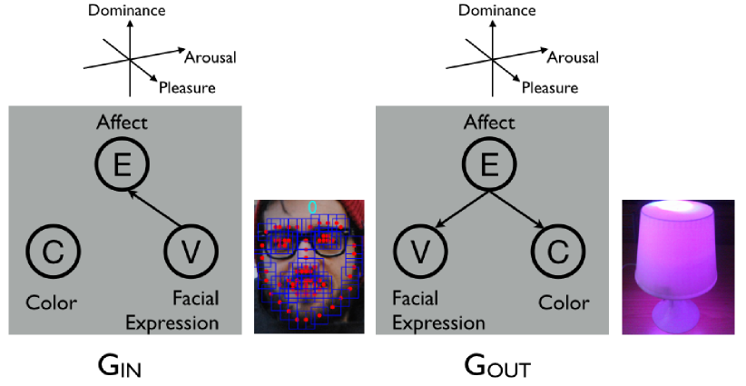
(b) (b) A PGM representation of IB

Figure 2: Synesthesia of facial expression $\mathbf{V}$ into the (lamp) color $\mathbf{C}$ as an Information Bottleneck problem. The displayed expression is represented as a random vector $\mathbf{V}$, computed on the basis of facial landmarks $\mathbf{L}$ (displayed as red dots superimposed on the face). (a) Transcoding $\mathbf{V}\mapsto\mathbf{C}$ is modelled as the search for a compressed representation of $\mathbf{V}$, namely the affect space $\mathbf{E}$, which achieves minimum redundancy while maintaining the mutual information $I(\mathbf{E};\mathbf{C})$ about the relevant variable $\mathbf{C}$, as high as possible. (b) The left graph $\mathcal{G}_{IN}$ encodes the compression process; the right graph $\mathcal{G}_{OUT}$ is the target model representing which relations should be maintained or predicted. The IB principle boils down to minimize the information maintained by $\mathcal{G}_{IN}$ and to maximize the information preserved by $\mathcal{G}_{OUT}$.

The second issue, which is tied in a subtle way to the previous one, grounds in the general and fundamental principle that an organism who maximizes the adaptive value of its actions given fixed resources should have internal representations of the outside world that are optimal in a very specific information-theoretic sense [2]. In a communicative action, this optimization problem is related to joint source channel coding, namely the task of encoding and transmitting information simultaneously in an efficient manner [7].

One route to do justice to both issues is the Information Bottleneck (IB), [26]. IB is an information-theoretic principle for coping with the extraction of relevant components of an “input” random variable $\mathbf{X}$, with respect to an “output” random variable $\mathbf{Y}$. This is performed by finding a bottleneck variable, that is a compressed, non-parametric and model-independent representation $\mathbf{T}$ of $\mathbf{X}$, that is most informative about $\mathbf{Y}$.

In our case the intuition is that the bottleneck variable $\mathbf{E}$ is suitable to capture the relevant affective aspects of the facial expression stimuli $\mathbf{V}$ that are informative about the output color stimulus $\mathbf{C}$ (cfr. Fig. 2(a)).

Denote $I(\mathbf{X};\mathbf{Y})$ the mutual information [7]. The original IB approach determines the auxiliary latent space $\mathbf{E}$ and related mapping $\mathbf{V}\mapsto\mathbf{E}$, such that the mutual information $I(\mathbf{V};\mathbf{E})$ is minimized (to achieve maximum compression), while relevant information $I(\mathbf{E};\mathbf{C})$ is maximized. Hence

$$\min_{\mathbf{V}\mapsto\mathbf{E}}I(\mathbf{V};\mathbf{E})-\beta I(\mathbf{E};\mathbf{C}),$$ (2)

where $\mathbf{V}\mapsto\mathbf{E}$ is the rule for creating the internal representation, and the positive parameter $\beta$ smoothly controls the tradeoff between compression and preserved relevant information.

The optimization principle in Eq. 2 is very abstract; also, no analytical solution is available. However, it has been shown by Friedman et al. [10] that the IB problem can be suitably reformulated in terms of directed Probabilistic Graphical Model (PGM, [16]) representation (cfr. Fig. 2(b)). A directed PGM is a graph-based representation where nodes denote RVs and arrows/arcs code conditional dependencies between RVs. Stated technically, the $\mathcal{G}$ structure encodes the set of conditional independence assumptions over the set of RVs $\{\mathbf{X}_{i}\}$ (called the local independencies, [16]) involved by the joint pdf $P(\{\mathbf{X}_{i}\})$ associated to $\mathcal{G}$. Then, the joint pdf factorizes according to $\mathcal{G}$ [16], that is $P$ is consistent with $\mathcal{G}$, $P\models\mathcal{G}$. Given a PGM $\mathcal{G}$, $I^{\mathcal{G}}=\sum_{i}I(\mathbf{X}_{i};Pa_{i}^{\mathcal{G}})$ denotes the information computed with respect to the pdf $P\models\mathcal{G}$ [10], where $Pa_{i}^{\mathcal{G}}$ stands for the ensemble of parents of node $\mathbf{X}_{i}$.

Under these circumstances, the IB principle (Eq. 2) can be shaped in the language of PGMs by considering two directed graphs $\mathcal{G}_{IN}$ and $\mathcal{G}_{OUT}$, together with the pdfs entailing such graphs, $Q\models\mathcal{G}_{IN}$ and $P\models\mathcal{G}_{OUT}$, respectively (cfr. Fig. 2(b)). Thus, the information that we would like to minimize is now given by $I^{\mathcal{G}_{IN}}$, where $I^{\mathcal{G}_{IN}}=I(\mathbf{V},\mathbf{E})$. The relevant information that we wish to preserve is specified by the target model $\mathcal{G}_{OUT}$, as $I^{\mathcal{G}_{OUT}}=I(\mathbf{E};\mathbf{V})+I(\mathbf{E};\mathbf{C})$. Assuming this, Eq. 2 can be rewritten,

$$\min_{\mathbf{V}\mapsto\mathbf{E}}I^{\mathcal{G}_{IN}}-\beta I^{\mathcal{G}_{OUT}}=\min_{Q}I(\mathbf{V};\mathbf{E})+\gamma D_{KL}(Q(\mathbf{V},\mathbf{E},\mathbf{C})||P(\mathbf{V},\mathbf{E},\mathbf{C}))$$ (3)

where $D_{KL}(Q(\mathbf{X})||P(\mathbf{X}))$ is the Kullback-Leibler divergence between distributions $Q$ and $P$ [7]. The scale parameter $\gamma$ balances the above two factors and is related to $\beta$ as $\beta=\gamma/(1+\gamma)$. In the limit $\gamma\to 0$ we are only interested in compressing the variable $\mathbf{V}$. When $\gamma\to\infty$ we concentrate on choosing a pdf $Q$ that is close to the distribution $P\models\mathcal{G}_{OUT}$:

$$P(\mathbf{V},\mathbf{C},\mathbf{E})=P(\mathbf{V}\mid\mathbf{E})P(\mathbf{C}\mid\mathbf{E})P(\mathbf{E}),$$ (4)

by minimizing $D_{KL}(Q(\mathbf{V},\mathbf{E},\mathbf{C})||P(\mathbf{V},\mathbf{E},\mathbf{C}))$.

It has been shown that iterative approximate solutions to Eq. 2, which cycle between determining $Q(\mathbf{E})$ and $Q(\mathbf{C}\mid\mathbf{E})$ for a fixed $Q(\mathbf{E}\mid\mathbf{V})$, and computing $Q(\mathbf{E}\mid\mathbf{V})$ for fixed $Q(\mathbf{E})$ and $Q(\mathbf{C}\mid\mathbf{E})$, are a formulation of the generalized Expectation-Maximization algorithm for clustering [23]. Clearly, this holds when the latent space $\mathbf{E}$ is a discrete space. Indeed, it is readily seen that at the extreme spectrum $\gamma\to\infty$, the minimization in Eq. 3 boils down to minimize $D_{KL}(Q(\mathbf{V},\mathbf{E},\mathbf{C})||P(\mathbf{V},\mathbf{E},\mathbf{C}))$ which is but one instance of the Variational Bayes method for learning the generative model $P\models\mathcal{G}_{OUT}$, as represented in the target model of Fig. 2(b).

When the transcoding operation relies upon a continuous latent space – as in our case – the IB approach represented in terms of $P\models\mathcal{G}_{OUT}$ is reminiscent of several latent factor models for paired data, such as Bayesian factor regression, Probabilistic Partial Least squares and Probabilistic CCA [16].

3 Methods

The IB approach provides a principled justification to the use of a mediating latent space for simulating computational synaestesia. After the learning stage, when the distribution factors of the target joint pdf are available, transcoding in Eq. 1 can be performed via the latent space $\mathbf{E}$:

$$\mathbf{e}\sim P(\mathbf{E}\mid\mathbf{V}=\mathbf{v}),\quad\mathbf{c}\sim P(\mathbf{C}\mid\mathbf{E}=\mathbf{e}).$$ (5)

It is worth remarking that learning procedures implementing optimization (2) or (3) have the goal of designing from scratch a latent space that is optimal with respect to the given constraints and the joint distribution, here $P(\mathbf{V},\mathbf{C})$. In the case study we are considering, conditions are slightly different. First, the latent space $\mathbf{E}$ is not constructed abstractly, but it should be chosen guided by psychological theories of emotion; this somehow simplifies some machine learning issues, for instance, the dimensionality of the space is not to be learned. Second, the joint pdf is not straightforwardly available.

As to the first issue, we assume a core affect representation. Core affect is a neurophysiological state that underlies simply feeling good or bad, drowsy or energised, and it can be experienced as free-floating, or mood, or can be attributed to some cause (and thereby begin an emotional episode) [20]. Thus, it is a continuous latent space and a suitable representation is provided by the PAD space proposed by Mehrabian and Russell [21]. Such space can be described along three nearly independent continuous dimensions: Pleasure-Displeasure (measured by $P$), Arousal-Nonarousal ($A$), and Dominance-Submissiveness ($D$); thus, $\mathbf{E}=\left[PAD\right]^{\intercal}$.

Note that, under the assumption of an actual affective state $\mathbf{E}=\mathbf{e}$, it is easy to show, by using Bayes’ rule and the joint pdf factorisation (4), that $P(\mathbf{V},\mathbf{C}\mid\mathbf{E})=P(\mathbf{V}\mid\mathbf{E})P(\mathbf{C}\mid\mathbf{E})$, thus $\mathbf{V}\mathrel{\perp\mspace{-10.0mu}\perp}\mathbf{C}\mid\mathbf{E}$. That is, if the affective state is given, then $\mathbf{V}$ and $\mathbf{C}$ are conditionally independent. The very issue here is thus obtaining the “mapping” probabilities $P(\mathbf{E}\mid\mathbf{V})$ and $P(\mathbf{C}\mid\mathbf{E})$. To this end, we can make the simplifying assumption of a Gaussian IB [5]. In this case an optimal compression $\mathbf{E}$ is obtained with a noisy linear transformation of $\mathbf{V}$:

$$\mathbf{e}=\mathbf{W}_{E}\mathbf{v}+\xi_{E},\quad\quad\xi_{E}\sim\mathcal{N}(\mathbf{0},\Sigma_{\xi_{E}}),$$ (6)

where $\xi_{E}$ is an additive noise term sampled from a zero-mean Gaussian pdf $\mathcal{N}(\mathbf{0},\Sigma_{\xi_{E}})$.

Similarly, the most natural choice for color is a continuous space; e.g., in studies concerning relationships between color and emotion the HSL space – defined on Hue ($H$), Saturation ($S$) and Luminance ($L$) – has been used [11, 14]. Thus, a generative model for mapping $P(\mathbf{V}\mid\mathbf{E})$ is

$$\mathbf{c}=\mathbf{W}_{C}\mathbf{e}+\xi_{C},\quad\quad\xi_{C}\sim\mathcal{N}(\mathbf{0},\Sigma_{\xi_{C}}).$$ (7)

Eqs. 6 and 7 nicely simplify the synaesthetic mapping to a pair of regressions on a joint latent space, however the second issue related to the actual availability of $P(\mathbf{V},\mathbf{C})$ must be taken into account. Needless to say, the use of a continuous affect space brings along a number of challenges. In the psychological literature, fleeting changes in the countenance of a face are considered to be “expressions of emotion” (EEs) and have been systematically investigated by Ekman [9] in a categorical perpsective. Ekman’s work has fostered a vaste amount of theoretical and empirical work, which has been particularly influent in the affective computing community [28]. Under these circumstances, finding the map $\mathbf{V}\mapsto\mathbf{E}$, has been mostly relied on a pattern recognition approach to infer emotions from expressions under the fundamental assumption of basic emotions, for example by considering the discrete set $\mathbf{E}=\{\text{joy},\text{sadness},\text{anger},\text{disgust},\text{surprise},\text{fear}\}$. By contrast, Eq. 6 assumes a probabilistic relationship between $\mathbf{E}$ and $\mathbf{V}$ where $\mathbf{E}$ is continuously defined.

A second problem to solve is related to Eq. 7, that is to learn the mapping $\mathbf{E}\mapsto\mathbf{C}$. In the past decades, only a few researchers investigated the relationship between color and emotion [27, 15, 3, 14, 25] (and often in the sense of emotion elicited by a colors and not the vice versa). In this case, the main problem is setting up a minimal training set which we derive from data available from the psychological literature. These issues are addressed in the following sections.

4 From face expression to mood

In this section we detail how we solve the problem of learning a probabilistic relationship between $\mathbf{E}$ and $\mathbf{V}$ where $\mathbf{E}$ is continuously defined according to the PAD model. To this end, we exploit results of experimental studies that have evaluated the PAD value of discrete emotion states, e.g., [12].

A very first step concerns with the facial landmark localisation, which can be summarised as follows. Denote $\mathbf{L}=\{\mathbf{l}^{1},\mathbf{l}^{2},\cdots,\mathbf{l}^{n}\}$ the locations of $n$ landmarking parts of the face, and $\mathbf{F}=\{\mathbf{f}^{1},\mathbf{f}^{2},\cdots,\mathbf{f}^{n}\}$ the measured detector responses, where $\mathbf{f}^{i}=\phi(\mathbf{l}^{i},\mathcal{I})$ is the response or feature vector provided by a local detector at location $\mathbf{l}^{i}$ in image or frame $\mathcal{I}$. Then, localisation can be solved by finding the value of $\mathbf{L}$ that maximises the probability of $\mathbf{L}$ given the responses from local detectors, namely $\mathbf{L}^{*}=\arg\max_{\mathbf{L}}P(\mathbf{L}|\mathbf{F})$. Following [8], we exploit a part-based framework that integrates an effective local representation based on sparse coding. Sparse coding has recently gained currency in face analysis (e.g.,[13, 1]). In particular:

$$\mathbf{L}^{*}=\arg\max_{L}\sum_{k=1}^{m}\int_{t}\prod_{i=1}^{n}P(\Delta\mathbf{l}^{i}_{k,t})P(\mathbf{l}^{i}|\mathbf{f}^{i})dt,$$ (8)

where the prior $P(\Delta\mathbf{l}^{i}_{k,t})$ accounts for the shape or global component of the model, and $P(\mathbf{l}^{i}|\mathbf{f}^{i}))$ for the appearance or local component. For what concerns the local component $P(\mathbf{l}^{i}|\mathbf{f}^{i})$, we resort to Histograms of Sparse Codes to sample patch responses $\mathbf{f}^{i}$, which we learn from facial images (see [8] for details).

For each image/frame we consider $40$ landmarks $\mathbf{L}=\left[\mathbf{l}^{1}\cdots\mathbf{l}^{40}\right]^{\intercal}$ as shown in Fig. 4, and we map them into a vector of visible expression parameters $\mathbf{V}$ by measuring the landmark displacements. This step, in a vein similar to Action Units approaches [9], is aimed at capturing the expression movements within local face region, such as mouth-bent, eye-open and eyebrow-raise, etc., as detailed in Tab. 4 [4].

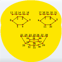
Figure 3: The 40 facial landmarks

Name	EP	Definition
Eyes height	$\mathbf{v}^{0}$	$(\mathbf{l}^{0}_{y}-\mathbf{l}^{1}_{y})*2$
Eyes / brows space	$\mathbf{v}^{1}$	$\mathbf{l}^{0}_{y}-\mathbf{l}^{13}_{y}+\frac{(\mathbf{l}^{16}_{y}-\mathbf{l}^{12}_{y})}{4}$
Eyebrow’s inner height	$\mathbf{v}^{2}$	$\mathbf{l}^{12}_{y}+\mathbf{v}^{1}-\mathbf{l}^{0}_{y}$
Eyebrow’s outer height	$\mathbf{v}^{3}$	$\mathbf{l}^{16}_{y}+\mathbf{v}^{1}-\mathbf{l}^{0}_{y}$
Mouth width	$\mathbf{v}^{4}$	$\mathbf{l}^{28}_{x}-\mathbf{l}^{22}_{x}$·
Mouth openness	$\mathbf{v}^{5}$	$\mathbf{l}^{31}_{y}-\mathbf{l}^{25}_{y}$
Mouth twist	$\mathbf{v}^{6}$	$\frac{\mathbf{l}^{28}_{y}-\mathbf{l}^{25}_{y}}{2}-\mathbf{l}^{22}_{y}$

Figure 4: Visual expression parameters (EP) via local landmark displacements

The extracted expression parameters $\mathbf{V}\in\mathbb{R}^{7}$ are put in correspondence to PAD values, $\mathbf{E}\in\mathbb{R}^{3}$, by using Eq. 6. In the current simulation, a multilinear ridge regression has been used, that is a penalized least squares method that adds a Gaussian prior to the parameters to encourage them to be small. Such model has interesting connection to latent variable space inference [16].

5 The color of mood

Here, we discuss some subtleties related to the mapping $\mathbf{E}\mapsto\mathbf{C}$ in order to learn the generative model of Eq. 7. Recall that we represent color as a random vector in HSL color space, i.e. $\mathbf{c}=\left[HSL\right]^{\intercal}$.

The seminal work investigating the relationship between color and emotion is that by Valdez and Mehrabian [27]. They mainly studied how saturation $S$ and luminance $L$ affect PAD. In [15, 3, 25] the emotions elicited by basic colors have been qualitative presented. Only recently in [14] a synthesis of these approaches has been proposed, aiming at allowing robots to express the intensity of emotions by coloring and blinking LED placed around their eyes. This work has the limit to resort to only two distinct values for both $S$ and $L$, and four values for the hue $H$, hence leading different emotions to be represented by the same color.

In our study, we propose a finer correspondence model, preserving maximum representativeness of the three components HSL. More precisely, as to $S$ and $L$, following [14], we invert the dependency of PAD values proposed in [27], while maintaining the obtained results. Define

$$P=0.69L+0.22S,\quad A=-0.31L+0.60S,\quad D=-0.76L+0.32S.$$ (9)

Then, $S$ and $L$ can be derived

$$\hat{\mathbf{c}}=(\mathbf{W}^{\intercal}\mathbf{W})^{-1}\mathbf{W}^{\intercal}\mathbf{e},$$ (10)

where $\hat{\mathbf{c}}=\begin{bmatrix}LS\end{bmatrix}^{\intercal}$, $\mathbf{W}=\begin{bmatrix}0.69&0.22\\ -0.31&0.60\\ -0.76&0.32\end{bmatrix}$, and $\mathbf{e}=\begin{bmatrix}PAD\end{bmatrix}^{\intercal}$.

Eq.10 provides a partial color mapping $\mathbf{E}\mapsto(S,L)$. To complete the picture we need to take into account hue values $H$. Unfortunately, the hue / PAD relation proposed in [27] cannot be inverted. We thus derive this component from Plutchik’s psycho-evolutionary emotion theory [19]. In his work, each emotion is associated to a given hue value, while saturation and luminance vary according to the emotion intensity (Fig. 6). As we need an association between PAD and hue values, we rely on the classification made by Mehrabian [21], adopting the PAD values of a subset of corresponding affective states, as tabulated in Tab. 6.

Eventually, PAD values and the corresponding HSL values, can serve, respectively, as feature and target sets for learning the multivariate linear regression model given in Eq. 7. As in the case of Eq. 6 this is accomplished via ridge regression.

Finally, the obtained HSL values are converted into RGB space. The latter step has a practical motivation. As discussed from the beginning, the realisation of the transcoding process has been experimented through the Mood Lamp, an affective object conceived as i) a sensing interface, namely a low-cost web camera / notebook communicating via USB with ii) a modified Ikea lamp, equipped with an Arduino UNO board to control an RGB LED (see Fig. 7).

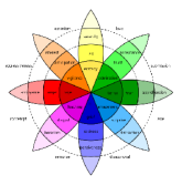
Figure 5: Plutchik’s wheel. Relationships between emotions and colors. Hue is associated to a specific emotion, while saturation and luminance determine its intensity.

Emotion	H	S	L	P	A	D
joy	60	67	100	0.81	0.51	0.46
ecstasy	60	67	100	0.62	0.75	0.38
fear	120	100	59	-0.64	0.60	-0.43
terror	120	100	50	-0.62	0.82	-0.43
amazement	203	100	88	0.16	0.88	-0.15
sadness	240	68	100	-0.63	-0.27	-0.33
boredom	300	22	100	-0.65	-0.62	-0.33
annoyance	0	45	100	-0.58	0.40	0.01
anger	0	100	100	-0.51	0.59	0.25
interest	29	45	100	0.64	0.51	0.17
vigilance	29	100	100	0.49	0.57	0.45

Figure 6: Color values of emotions according to the Plutchik’s wheel and their associations to Mehrabian [21] scores of Pleasure, Arousal and Dominance.

Figure 7: Color control: the actual color stimulus is generated through a modified Ikea lamp, where the RGB LED is controlled by an Arduino UNO board.

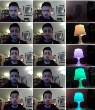
Figure 8: Experimental results of transconding using the Mood Lamp.

6 Conclusion and further outlooks

We have discussed how the IB framework provides a parsimonious and principled account of using a latent affect space to mediate the rechanneling between different stimuli. As a final comment, we think it appropriate to remark that the general formalism which is expounded here admits a far wider range of applicability than that to which it has been presented in this work. The framework could be usefully adopted for current affective computing systems that more and more relying on the availability of different sensors (e.g., for monitoring autonomic activity) and brain interfaces [28]. Indeed, such systems are confronted with the issue of finding relations in high-dimensional and heterogeneous data spaces, one example being data fusion among several others which would emerge from the application of this approach to concrete instances.

References

- [1] Adamo, A., Grossi, G., Lanzarotti, R.: Local features and sparse representation for face recognition with partial occlusions. In: 20th IEEE Int. Conf. on Image Processing (ICIP). pp. 3008–3012 (Sept 2013)
- [2] Bialek, W., van Steveninck, R.R.R., Tishby, N.: Efficient representation as a design principle for neural coding and computation. In: IEEE International Symposium on Information Theory. pp. 659–663. IEEE (2006)
- [3] Birren, F.: Color Psychology and Color Therapy. Kessinger Publishing (2006)
- [4] Broekens, J., Brinkman, W.: Affectbutton: A method for reliable and valid affective self-report. Int. J. Hum.-Comput. Stud. 71(6), 641–667 (2013)
- [5] Chechik, G., Globerson, A., Tishby, N., Weiss, Y.: Information bottleneck for gaussian variables. Journal of Machine Learning Research 6, 165–188 (2005)
- [6] Collier, G.L.: Affective synesthesia: Extracting emotion space from simple perceptual stimuli. Motivation and emotion 20(1), 1–32 (1996)
- [7] Cover, T., Thomas, J.: Elements of Information Theory. Wiley and Sons, New York, N.Y. (1991)
- [8] Cuculo, V., Lanzarotti, R., Boccignone, G.: Using sparse coding for landmark localization in facial expressions. In: 5th European Workshop on Visual Information Processing (EUVIP). pp. 1–6 (Dec 2014)
- [9] Ekman, P.: Facial expression and emotion. American Psychologist 48(4), 384 (1993)
- [10] Friedman, N., Mosenzon, O., Slonim, N., Tishby, N.: Multivariate information bottleneck. In: Proceedings of the Seventeenth conference on Uncertainty in artificial intelligence. pp. 152–161 (2001)
- [11] Gao, X.P., Xin, J.: Investigation of human’s emotional responses on colors. Color Research & Application 31(5), 411–7 (2006)
- [12] Hoffmann, H., Scheck, A., Schuster, T., Walter, S., Limbrecht, K., Traue, H.C., Kessler, H.: Mapping discrete emotions into the dimensional space: An empirical approach. In: IEEE International Conference on Systems, Man, and Cybernetics (SMC). pp. 3316–3320. IEEE (2012)
- [13] Jeni, L., Girard, J., Cohn, J., De la Torre, F.: Continuous AU intensity estimation using localized, sparse facial feature space. In: 10th IEEE Int. Conf. and Workshops Automat. Face Gesture Recogn. pp. 1–7 (April 2013)
- [14] Kim, M., Lee, H., Park, J., Jo, S., Chung, M.: Determining color and blinking to support facial expression of a robot for conveying emotional intensity. In: Int’l Symposium on Robot and Human Interactive Communication, RO-MAN. pp. 219–24 (2008)
- [15] Mahnke, F.H.: COLOR, Environment, & Human Response. John Wiley & Sons (1996)
- [16] Murphy, K.P.: Machine learning: a probabilistic perspective. MIT press, Cambridge, MA (2012)
- [17] Osgood, C.E., Suci, G.J., Tannenbaum, P.H.: The measurement of meaning. University of Illinois Press (1964)
- [18] Pessoa, L.: On the relationship between emotion and cognition. Nature Reviews Neuroscience 9(2), 148–158 (2008)
- [19] Plutchik, R.: Emotion: Theory, Research and Experience. Acad. Pr (1980)
- [20] Russell, J.A.: Core affect and the psychological construction of emotion. Psychological review 110(1), 145 (2003)
- [21] Russell, J.A., Mehrabian, A.: Evidence for a three-factor theory of emotions. Journal of research in Personality 11(3), 273–294 (1977)
- [22] Scheirer, J., Picard, R.: Affective objects. MIT Media lab Technical Rep. 524 (2000)
- [23] Slonim, N., Weiss, Y.: Maximum likelihood and the information bottleneck. In: Advances in neural information processing systems. pp. 335–342 (2002)
- [24] Spence, C.: Crossmodal correspondences: A tutorial review. Attention, Perception, & Psychophysics 73(4), 971–995 (2011)
- [25] Suk, H.J., Irtel, H.: Emotional response to color across media. Color Research & Application 35(1), 64–77 (2010)
- [26] Tishby, N., Pereira, F.C., Bialek, W.: The information bottleneck method. In: The 37th Allerton Conference on Communication, Control, and Computing (1999)
- [27] Valdez, P., Mehrabian, A.: Effects of color on emotions. Journal of Experimental Psychology: General 123(4), 394 (1994)
- [28] Vinciarelli, A., Pantic, M., Heylen, D., Pelachaud, C., Poggi, I., D’Errico, F., Schroeder, M.: Bridging the gap between social animal and unsocial machine: A survey of social signal processing 3(1), 69–87 (2012)
- [29] Vitale, J., Williams, M.A., Johnston, B., Boccignone, G.: Affective facial expression processing via simulation: A probabilistic model. Biologically Inspired Cognitive Architectures Journal 10, 30–41 (2014)
- [30] Ward, J.: Emotionally mediated synaesthesia. Cognitive Neuropsychology 21(7), 761–772 (2004)