Winding number excitation detects phase transition in one-dimensional $XY$ model with variable interaction range

Abstract

We numerically study the critical behavior of the one-dimensional $XY$ model of the size $N$ with variable interaction range $L$. As expected, the standard local order parameter of the magnetization is shown to well detect the mean-field type transition which occurs at any nonzero value of $L/N$. The system is particularly interesting since the underlying one-dimensional structure allows us to study the topological excitation of the winding number across the whole system even though the system shares the mean-field transition with the globally-coupled system. We propose a novel nonlocal order parameter based on the width of the winding number distribution which exhibits a clear signature of the transition nature of the system.

I Introduction

The $XY$ model is one of typical model systems that have been widely studied in the arena of statistical physics ref:XYreview . Most existing studies so far have been performed in the regular lattice structures of one ref:XY_1D , two ref:XY_2D , three ref:XY_3D , and four ref:XY_4D dimensions. In particular, two-dimensional (2D) $XY$ model has been found to exhibit the famous Berezinskii-Kosterlitz-Thouless (BKT) transition ref:XY_2D , and the all-to-all globally-coupled $XY$ system has been known to exhibit the mean-field (MF) type phase transition ref:XY_MF . Also, recent progress in complex network research has made the interplay between connection structure of interacting spins and the nature of phase transition a central topic in statistical physics ref:XY_complexnetwork ; ref:XY_small . Differently from most previous studies, we investigate in this paper the one-dimensional (1D) $XY$ model with variable interaction range and explore how the interaction range affects the collective critical behavior of the model. The underlying 1D topology of the system allows us to study the winding number excitation that has been known to exist in the system with local/nonlocal interaction ref:twiststate ; ref:nonlocal_Hong_Kim . We propose a novel nonlocal order parameter based on the distribution of the winding number excitation, which is found to successfully exhibit a clear signature of the phase transition.

The present paper consists of five sections. Section II introduces the model and in Sec. III we explore thermodynamic behavior of the model, by measuring the standard quantities such as magnetization, specific heat, susceptibility, and Binder’s cumulant to detect the phase transition. In Sec. IV, which contains the key part of the present paper, we define the winding number for a given configuration of the phase variables, and investigate the behavior of its distribution depending on the system size and temperature. Based on the observation of the winding number distribution function, a novel nonlocal order parameter is introduced and used to successfully detect the phase transition. Finally, a brief summary follows in Sec. V.

II Model

We study the 1D $XY$ model of $N$ spins described by the Hamiltonian

$$H=-\frac{J}{2L}\sum_{i=1}^{N}\sum_{j=i-L}^{i+L}\cos(\phi_{i}-\phi_{j}),$$ (1)

where $\phi_{i}\in(-\pi,\pi)$ is the phase angle variable of the $i$th spin with the periodic boundary condition $\phi_{i+N}=\phi_{i}$, and $L$ is the interaction range in one side so that each spin interacts with total $2L$ nearest-neighbor spins in both sides. We take the ferromagnetic coupling with the positive strength $(J>0)$, which makes the neighbor spins favor their phase difference to be minimized. The typical 1D $XY$ model with the nearest-neighbor interaction corresponds to the case of $L=1$, and the globally-coupled $XY$ model with all-to-all couplings is achieved when $L=N/2-1$, respectively. We in the present paper investigate the collective behavior of the model given by Eq. (1), varying the interaction range $L$, which is a key control parameter that passes from the short-range ($L/N\rightarrow 0$) to the infinite-range ($L/N\rightarrow 1/2$) regimes in the thermodynamic limit of $N\rightarrow\infty$.

After suitable normalization of time, energy, and temperature, the first-order Langevin-type equations of motion of the system read

$$\dot{\phi_{i}} = -\frac{\partial H}{\partial\phi_{i}}+\eta_{i},$$ (2)

$$= -\frac{1}{2L}\sum_{j=i-L}^{i+L}\sin(\phi_{i}-\phi_{j})+\eta_{i},$$

where the dimensionless thermal noise $\eta_{i}$ satisfies

$$\langle\eta_{i}(t)\eta_{j}(t^{\prime})\rangle=2T\delta(t-t^{\prime})$$ (3)

at the dimensionless temperature $T$ in units of $J/k_{B}$ with the Boltzmann constant $k_{B}$. We have taken the overdamped regime with the inertia term (containing $\ddot{\phi_{i}}$) neglected as in Ref. ref:PRB_35_8528, where a condensed matter system (smectic liquid-crystal) has been studied. Equation (2) at zero temperature $(T=0)$ has also been used to describe the system of the 1D coupled oscillators with variable interaction range ref:nonlocal_Hong_Kim . If one is only interested in equilibrium behavior as in the present study, one can use the Mont-Carlo (MC) simulation method instead.

We note that the 1D system with short-range interaction does not exhibit any long-range order at finite temperature ref:XY_1D . On the other hand, when the dimensionality of the system is higher than the lower critical dimension 2, the celebrated Mermin-Wagner theorem ref:mermin-wagner cannot disprove the existence of the long-range order, as typically exemplified in 3D ref:XY_3D , 4D ref:XY_4D , and globally-coupled ref:XY_MF $XY$ models. In this context, it is natural to have the following questions: Is there a critical interaction range $(L/N)_{c}$ beyond which a finite-temperature phase transition starts to occur? If so, does the phase transition always belong to the MF universality class? To answer these questions, we study the critical behavior of the model, first measuring some standard quantities for various values of $L$ and $N$, which is presented in next section.

III Thermodynamic Behavior

In this section we numerically study the thermodynamic behavior of the system, with particular attention paid to the emergence of the phase transition at finite values of the interaction range $L$. It is possible to numerically investigate equilibrium behavior of the system in two different ways: numerical integration of equations of motion Eq. (2) and MC simulation based on the Hamiltonian Eq. (1). It is straightforward to show that both numerical methods are equivalent to each other as long as only equilibrium behaviors are concerned: the steady-state solution of the Fokker-Planck equation based on Eq. (2) is simply the Boltzmann distribution $P\sim\exp(-H/k_{B}T)$ with the Hamiltonian in Eq. (1) Fokker_Planck . Since the MC simulations usually run much faster than direct integration of stochastic differential equations, we here use the former with the standard Metropolis local update algorithm and measure various quantities of interest. In the MC simulations, all quantities are measured over $10^{7}$-$10^{8}$ MC steps after equilibration over the initial $10^{6}$ MC steps.

We measure the equilibrium magnetization defined as

$$m_{\phi}=\left\langle\left|\frac{1}{N}\sum_{j=1}^{N}e^{i\phi_{j}}\right|\right\rangle,$$ (4)

where $\langle\cdots\rangle$ denotes the thermal average. The behavior of the magnetization $m_{\phi}$ is shown as a function of the temperature $T$, varying the value of $L$ to keep the ratio $L/N$ unchanged [see Fig. 1]. We find that the magnetic ordering ($m_{\phi}>0$) occurs at $T\lesssim 0.5$ for $L/N=0.4$, as shown in Fig. 1(a). The signature of the transition from the disordered phase ($m_{\phi}=0$) to the ordered one ($m_{\phi}>0$) becomes clearer as the system size $N$ increases. We also measure the magnetization for smaller value, $L/N=0.1$ [see Fig. 1(b)] and $L/N=0.05$ (not shown here), and find that the two cases also show the magnetic ordering for $T\lesssim 0.5$, for sufficiently large system sizes. The behavior of the magnetization shown in Fig. 1 suggests that the finite-temperature phase transition occurs at any nonzero value of $L/N$. In other words, we expect that the critical value of the interaction range beyond which the phase transition occurs at a nonzero critical temperature satisfies $(L/N)_{c}=0$ in the thermodynamic limit.

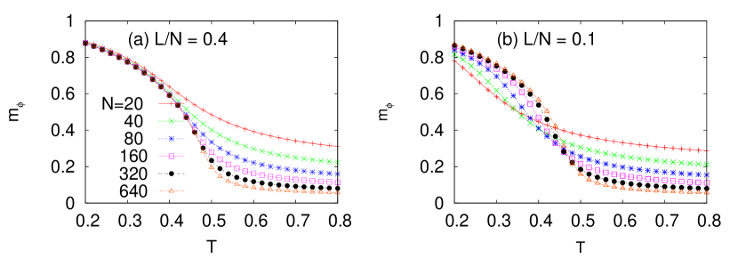
Figure 1: (Color online) Magnetization $m_{\phi}$ is plotted as a function of the temperature $T$ for various system sizes $N$ and interaction ranges $L$ for (a) $L/N=0.4$ and (b) $L/N=0.1$, respectively.

To see it further, we also investigate other standard quantities such as the specific heat $c_{v}$, susceptibility $\chi$, and Binder’s fourth-order cumulant $U_{B}$ ref:Binder , defined by

$$c_{v} \equiv \frac{1}{Nk_{B}T^{2}}\Bigg{(}\langle H^{2}\rangle-\langle H\rangle^{2}\Bigg{)},$$ (5)

$$\chi \equiv \frac{N}{k_{B}T}\Bigg{(}\langle m^{2}_{\phi}\rangle-\langle m_{\phi}\rangle^{2}\Bigg{)},$$ (6)

$$U_{B} \equiv 1-\frac{\langle m^{4}_{\phi}\rangle}{3\langle m^{2}_{\phi}\rangle^{2}},$$ (7)

where $H$ is the Hamiltonian in Eq. (1). Figures 2 and 3 show $c_{v}$ and $U_{B}$ as functions of $T$ for $L/N=0.4$ and $L/N=0.1$, respectively. We find that both quantities, $c_{v}$ and $U_{B}$, strongly support the emergence of the phase transition at $T\approx 0.5$ for both $L/N=0.4$ and $0.1$. Although not shown here $\chi(T)$ has a peak which shifts towards $T_{c}\approx 0.5$ as the system size is increased both for $L/N=0.4$ and 0.1. We also investigated for the case of $L/N=0.05$ (not shown), and obtained the same conclusion if we focus on larger system sizes.

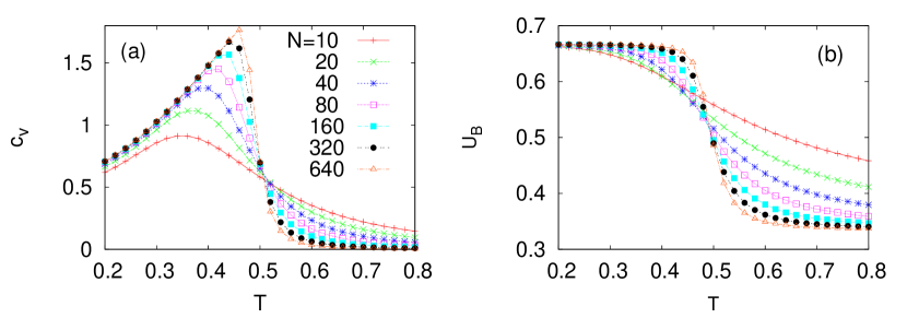
Figure 2: (Color online) (a) Specific heat $c_{v}$ and (b) Binder’s cumulant $U_{B}$ versus the temperature $T$ for various system sizes $N$. The interaction rage $L$ is chosen to yield the same value of the ratio $L/N=0.4$.

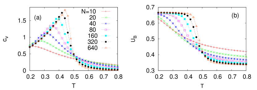
Figure 3: (Color online) (a) $c_{v}$ and (b) $U_{B}$ versus $T$ for $L/N=0.1$. For comparison, see Fig. 2 for $L/N=0.4$.

We turn our attention to the universality class of the phase transition, and consider the critical behavior of the magnetization characterized by

$$m_{\phi}\sim(T-T_{c})^{\beta}$$ (8)

with the critical exponent $\beta$ and the critical temperature $T_{c}$ in the thermodynamic limit. According to the finite-size scaling theory ref:FSS , we expect that $m_{\phi}$ in a finite-sized system satisfies the scaling form

$$m_{\phi}=N^{-\beta/\bar{\nu}}f\bigl{(}(T{-}T_{c})N^{1/{\bar{\nu}}}\bigr{)},$$ (9)

where $\bar{\nu}$ is the critical exponent that describes the critical behavior of the correlation volume $\xi_{v}\sim\xi^{d}$ in $d$ dimensions: $\xi_{v}\sim|T-T_{c}|^{-\bar{\nu}}$ ref:xi_v . The scaling function $f(x)$ with the scaling variable $x\equiv(T-T_{c})N^{1/\bar{\nu}}$ has limiting behaviors: $f(x)\sim x^{\beta}$ as $x\rightarrow 0$ and $f(x)\sim{\rm{const.}}$ as $x\rightarrow+\infty$. At criticality ($T=T_{c}$), the magnetization reduces to

$$m_{\phi}\sim N^{-\beta/\bar{\nu}}.$$ (10)

To estimate the exponents $\beta$ and $\bar{\nu}$ we plot $m_{\phi}$ as a function of the size $N$ in the log-log scale (not shown), and measure its slope, which gives us the exponent $\beta/\bar{\nu}$. We also check the finite-size scaling relation directly by plotting $m_{\phi}N^{\beta/\bar{\nu}}$ versus $(T-T_{c})N^{1/\bar{\nu}}$, controlling the values of $\beta/\bar{\nu}$ and $\bar{\nu}$ [see Fig. 4(a)]. We find that the scaling function $f(x)$ converges to a constant for large $x$, and behaves as $x^{\beta}$ for small $x$ as expected. The numerical findings shown in Fig. 4(a) is then summarized as

$$\beta/\bar{\nu}=1/4~{}~{}{\mbox{and}}~{}~{}\bar{\nu}=2,$$ (11)

which yields $\beta=1/2$. This result implies that the nature of the phase transition for $L/N=0.4$ is the same as that of the MF transition ref:XY_MF . The crossing of the specific heat $c_{v}$ at $T_{c}$ shown in Fig. 2(a) and Fig. 3(a) also implies that the specific heat exponent $\alpha=0$, in accord with the MF universality class ref:XY_small . We also examined the case for the smaller value of $L/N=0.1$ [see Fig. 4(b)] and $L/N=0.05$ (not shown), and obtained the same result, which suggests that the mean-field nature of phase transitions should be robust for any nonzero value of $L/N$.

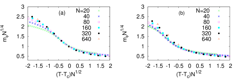
Figure 4: (Color online) Finite-size scaling collapse of the magnetization $m_{\phi}$: $m_{\phi}N^{\beta/\bar{\nu}}$ versus $(T-T_{c})N^{1/\bar{\nu}}$ for (a) $L/N=0.4$ and (b) $L/N=0.1$. With $T_{c}=0.5$, $\beta/\bar{\nu}=1/4$, and $\bar{\nu}=2$ chosen, good quality of scaling collapse of data is achieved.

IV Winding number excitation and a nonlocal order parameter

Recently, the emergence of twisted wave in the system of coupled oscillators with local/nonlocal interaction has been reported ref:twiststate ; ref:nonlocal_Hong_Kim . We note that the development of the twisted wave in dynamic models has the same physical origin as the winding number excitation in the 1D $XY$ model. In this section, we measure the winding number across the system in equilibrium for each sample and compute its probability distribution function by using a large-size ensemble of samples. We define the winding number $q$ for a given phase configuration by

$$q\equiv\frac{1}{2\pi}\sum_{i=1}^{N}{\mbox{mod}}(\phi_{i+1}-\phi_{i}),$$ (12)

where ‘mod’ denotes that the phase difference $\phi_{i+1}-\phi_{i}$ is measured modulo $2\pi$ and the periodic boundary condition $\phi_{N+1}=\phi_{1}$ is used. It is to be noted that the gapless spin-wave-type excitation can occur without changing the winding number. This reminds us the topological excitation of vortices in the conventional 2D $XY$ model ref:XYreview ; ref:XY_2D .

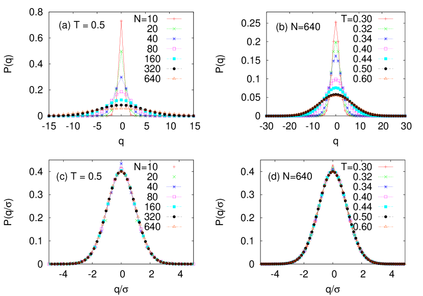
Figure 5: (Color online) Probability distribution function $P(q)$ of the winding number $q$ (a) at $T=0.5$ for various system sizes $N$ and (b) for a given size $N=640$ at various temperatures $T$. For each $P(q)$ the width of the distribution $\sigma(N,L,T)$ is computed and then used to scale the horizontal axis as shown in (c) and (d), each obtained from (a) and (b), respectively. For (a)-(d), $L/N=0.4$ has been used.

From the observation of the standard thermodynamic quantities in Sec. III, the system surely undergoes a single phase transition. Accordingly, we expect that the existence of the phase transition should also alter the pattern of the winding number excitation in some way at the observed critical temperature $T_{c}\approx 0.5$. We measure the probability distribution function of the winding numbers to see a signature of the phase transition, after sufficient equilibration procedure. Figure 5(a) shows the distribution $P(q)$ for various system sizes $N$ at the critical temperature $T_{c}(=0.5)$. We find that the width of the distribution function $P(q)$ systematically changes, as the system size $N$ is increased. The inversion symmetry $P(-q)=P(q)$ is easily understood since the system has no reason to prefer clockwise winding to counterclockwise one (and vice versa). The temperature dependence of the distribution $P(q)$ is also investigated at a given system size $N=640$ [see Fig. 5(b)]. Again, we observe that the width of the distribution changes as $T$ is varied. In order to check the possibility of the scaling of the winding number distribution function, we measure the standard deviation $\sigma$ defined by

$$\sigma\equiv\sqrt{\langle q^{2}\rangle-\langle q\rangle^{2}},$$ (13)

where $\langle q^{2}\rangle=\int q^{2}P(q)dq$ and $\langle q\rangle=\int qP(q)dq$. We then scale the horizontal axis in Fig. 5(a) and (b) by using the scaling variable $q/\sigma$ with $\sigma$ numerically computed for given values of $N$, $L$, and $T$. It is shown very clearly that after the winding number $q$ is scaled by the width $\sigma$ of the distribution function, all the curves are put on top of each other as displayed in Fig. 5(c) and (d), obtained from Fig. 5(a) and (b), respectively. Our observation of the collapse of the winding number distributions strongly suggests that the width $\sigma(N,L,T)$ of the distribution function can successfully represent the whole distribution function and thus will be used below for further analysis to study critical behavior in the system.

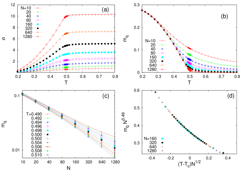
Figure 6: (Color online) (a) Standard deviation $\sigma$ is plotted as a function of the temperature $T$ for various system sizes $N$. (b) The newly defined nonlocal order parameter $m_{q}$ in Eq. (14) versus $T$ for various values of $N$. (c) $m_{q}$ versus $N$ in log-log scale clearly exhibits the power-law decay form at $T=T_{c}\approx 0.5$, with the slope corresponding to $\beta_{q}/\bar{\nu}_{q}=0.49$. (d) Finite-size scaling collapse of $m_{q}$ yields $\bar{\nu}_{q}=2.00(5)$. From (c) and (d), we estimate $T_{c}=0.500(3)$, $\beta_{q}/\bar{\nu}_{q}=0.49(4)$ and $\bar{\nu}_{q}=2.00(5)$. All results in (a)-(d) are for $L/N=0.4$.

In Fig. 6(a) we show $\sigma$ as a function of $T$ for various system sizes with $L/N=0.4$ fixed. From the central-limit theorem for the independent random variables, we expect that $P(q)$ at infinite temperature has $\sigma\sim\sqrt{N}$. In order to compensate such a behavior, we define the normalized width $s\equiv\sigma/\sqrt{N}$, and introduce a new quantity $m_{q}$ defined by

$$m_{q}\equiv s_{\infty}-s,$$ (14)

where $s_{\infty}\equiv s(N\rightarrow\infty,T\rightarrow\infty)$. From Fig. 6(a), it is expected that $m_{q}\rightarrow 0$ from above in the high-temperature limit and $m_{q}>0$ in the low-temperature regime, hopefully playing the role of the order parameter. The calculation of the value of $s_{\infty}$ is straightforward since the phase difference of the nearest neighbors $\phi_{i+1}-\phi_{i}$ simply becomes an independent random variable due to the lack of any spatial correlation in the high-temperature limit. In other words, $x_{i}\equiv\mod(\phi_{i+1}-\phi_{i})$ is independent from each other and randomly distributed in $x_{i}\in(-\pi,\pi]$. From the symmetry of the distribution we get $\langle q\rangle=0$, and the second moment $\langle q^{2}\rangle$ is computed as

$$\langle q^{2}\rangle = \frac{1}{4\pi^{2}}\Bigg{\langle}\Bigg{(}\sum_{i=1}^{N}x_{i}\Bigg{)}^{2}\Bigg{\rangle}$$ (15)

$$= \frac{N}{4\pi^{2}}\int_{-\pi}^{\pi}P(x)x^{2}dx=\frac{N}{12},$$

where $P(x)$ is the uniform probability distribution function for $x$ and the cross terms $x_{i}x_{j}~{}(i\neq j)$ has given null contribution from the independence between $x_{i}$ and $x_{j}$ at infinite temperature. Consequently, we get $\sigma=\sqrt{\langle q^{2}\rangle-\langle q\rangle^{2}}=\sqrt{N}/(2\sqrt{3})$ in the high-temperature limit, yielding $s_{\infty}=\sigma/\sqrt{N}=1/(2\sqrt{3})\approx 0.288675$. We then plot Fig. 6(b) for $m_{q}$ versus $T$, which looks very much similar to the standard order parameter $m_{\phi}$ in Fig. 1. Finite-size scaling ansatz then allows us to expect the existence of the scaling function given by

$$m_{q}=N^{-{\beta_{q}}/\bar{\nu}_{q}}g\bigl{(}(T-T_{c})N^{1/\bar{\nu}_{q}}\bigr{)},$$ (16)

where $g(x)$ is a scaling function that behaves as $g(x)\sim x^{\beta_{q}}$ as $x\rightarrow 0$, and $g(x)\sim{\mbox{const.}}$ as $x\rightarrow+\infty$. At criticality $(T=T_{c})$, the new nonlocal order parameter $m_{q}$ is expected to show the power-law behavior: $m_{q}\sim N^{-\beta_{q}/\bar{\nu}_{q}}$. On the basis of the prediction, we detect the exponents $\beta_{q}$ and $\bar{\nu}_{q}$, by plotting $m_{q}$ as a function of $N$ for various $T$, where the slope at $T_{c}$ gives the value of $\beta_{q}/\bar{\nu}_{q}$ [see Fig. 6(c)]. If only the large system sizes ($N\geq 160$) are used, we find that the curves follow the power-law form in Fig. 6(c) at $T=0.497$-$0.502$ with the slopes $\beta_{q}/\bar{\nu}_{q}=0.45$-$0.52$. For temperatures outside of this range, the curves exhibit clear deviations from the power-law form. The best fit to the power-law form is obtained at $T=0.500$ and $\beta_{q}/\bar{\nu}_{q}=0.49$, and thus we conclude $T_{c}=0.500(3)$ and $\beta_{q}/\bar{\nu}_{q}=0.49(4)$. The exponent $\bar{\nu}_{q}$ is obtained from the data collapse: Figure 6 (d) shows the behavior of $m_{q}N^{\beta_{q}/\bar{\nu}_{q}}$ against $(T-T_{c})N^{1/\bar{\nu}_{q}}$, where $\beta_{q}/\bar{\nu}_{q}=0.49$ and $\bar{\nu}_{q}=2.00$ at $T_{c}=0.500$ are used for the best collapse, yielding $\beta_{q}=0.98(11)$. It is particularly important to recognize that our new nonlocal order parameter based on the topological winding number excitation gives the correlation exponent $\bar{\nu}_{q}=2$, identical to $\bar{\nu}=2$ previously confirmed for the standard local magnetization order parameter $m_{\phi}$. However, we believe that further study is required to understand the value of $\bar{\beta}_{q}\approx 0.98$ which is very close to unity. We also examine results for $L/N=0.1$ and $L/N=0.05$ (not shown here); although not as clear as for $L/N=0.4$, we are able to confirm the same values of exponents as long as sufficiently bigger system sizes are used.

V Summary

In summary, we have numerically investigated the critical behavior of the 1D $XY$ model of $N$ spins with variable interaction range $L$. It has been confirmed that the critical interaction range beyond which the phase transition starts to occur at a nonzero finite temperature is very small, and presumably $(L/N)_{c}=0$. The nature of the transition has been examined by measuring standard quantities such as the magnetization, specific heat, susceptibility, and Binder cumulant. All measured quantities unanimously suggest the transition is of the mean-field type at any nonzero value of $L/N$. The underlying one-dimensional topology of the system makes it possible to study the winding number excitation. By systematically examining the probability distribution function of the winding number excitation, we have suggested a novel nonlocal order parameter $m_{q}$ based on the width of the winding number distribution function. We show that our new order parameter $m_{q}$ can successfully detect the phase transition and its nature.

References

- (1) For a general review see, e.g., P. Minnhagen, Rev. Mod. Phys. 59 1001 (1987).
- (2) S. De Nigris and X. Leoncini, EPL 101, 10002 (2013); Phys. Rev. E 88, 012131 (2013).
- (3) V.L. Berezinskii, Zh. Eksp. Teor. Fiz. 61, 1144 (1972) [Sov. Phys. JETP 34 610 (1972)]; J.M. Kosterlitz and D.J. Thouless, J. Phys. C 5, L124 (1972); 6, 1181 (1973); X. Leoncini, A.D. Verga, and S. Ruffo, Phys. Rev. E 57, 6377 (1998).
- (4) Y.-H. Li and S. Teitel, Phys. Rev. B 40, 9122 (1989); B.J. Kim, L.M. Jensen, and P. Minnhagen, Physica B 284, 413 (2000).
- (5) L.M. Jensen, B.J. Kim, and P. Minnhagen, Physica B 284, 455 (2000).
- (6) M. Antoni and S. Ruffo, Phys. Rev. E 52, 2361 (1995); A. Campa, T. Dauxois, and S. Ruffo, Phys. Rep. 480, 57 (2009).
- (7) S.N. Dorogovtsev, A.V. Goltsev, and J.F.F. Mendes, Rev. Mod. Phys. 80, 1275 (2008).
- (8) B.J. Kim, H. Hong, P. Holme, G.S. Jeon, P. Minnhagen, and M.Y. Choi, Phys. Rev. E 64, 056135 (2001); K. Medvedyeva, P. Holme, P. Minnhagen, and B.J. Kim, ibid. 67, 036118 (2003).
- (9) L.S. Tsimring, N.F.Rulkov, M.L. Larsen, and M. Gabbay, Phys. Rev. Lett. 95, 014101 (2005); D.A. Wiley, S.H. Strogatz, and M. Girvan, Chaos 16, 015103 (2006); T. Girnyk, M. Hasler, and Y. Maistrenko, Chaos 22, 013114 (2012).
- (10) H. Hong and B.J. Kim, J. Korean Phys. Soc. 64, 954 (2014).
- (11) R. Loft and T. A. DeGrand, Phys. Rev. B 35, 8528 (1987).
- (12) N.D. Mermin and H. Wagner, Phys. Rev. Lett. 17, 1133 (1966); P. Bruno, ibid. 87, 137103 (2001).
- (13) H. Risken, The Fokker-Planck Equation (Springer-Verlag, Berlin, 1984); B.J. Kim, P. Minnhagen, and P. Olsson, Phys. Rev. B 59, 11506 (1999).
- (14) K. Binder and D. W. Heermann, Monte Carlo Simulation in Statistical Physics, 2nd ed. (Springer-Verlag, Berlin, 1992).
- (15) M.E. Fisher and M.N. Barber, Phys. Rev. Lett. 28, 1516 (1972).
- (16) R. Botet. R. Jullien, and P. Pfeuty, Phys. Rev. Lett. 49, 478 (1982).