Modified weak measurements for detecting photonic spin Hall effect

Abstract

Weak measurement is an important technique for detecting the tiny spin-dependent splitting in photonic spin Hall effect. The weak measurement is only valid when the probe wavefunction remains almost undisturbed during the procedure of measurements. However, it does not always satisfy such condition in some practical situations, such as in the strong-coupling regime or the preselected and postselected states are nearly orthogonal. In this paper, we develop a modified weak measurement for detecting photonic spin Hall effect when the probe wavefunction is distorted. We find that the measuring procedure with preselected and postselected ensembles is still effective. This scheme is important for us to detect the photonic spin Hall effect in the case where neither weak nor strong measurements can detect the spin-dependent splitting. The modified theory is valid not only in weak-coupling regime but also in the strong-coupling regime, and especially in the intermediate regime. The theoretical models of conventional weak measurements and modified weak measurements are established and compared. We show that the experimental results coincide well with the predictions of the modified theory.

I Introduction

Weak measurements as an extension of quantum measurements were first introduced by Aharonov, Albert, and Vaidman Aharonov1988 . In quantum measurements, the observable of system couples a probe state with a pointer whose value can be read out by a meter. In general, the conventional quantum measurements involve in a process of strong coupling with the probe wavefunction is distorted. Weak measurements suggest that the coupling between the observable and the probe state is weak and the probe wavefunction remains almost undisturbed. The weak value of an observable $\hat{A}$ outside the eigenvalue spectrum can be obtained and the results are much larger than any eigenvalues of the quantum system. It is shown that the weak value $A_{w}$ can be formed as a simple expression

$$A_{w}=\frac{\langle\psi_{f}|\hat{A}|\psi_{i}\rangle}{\langle\psi_{f}|\psi_{i}\rangle},$$ (1)

in which $|\psi_{i}\rangle$ and $|\psi_{f}\rangle$ are the preselected and postselected states, respectively Aharonov1988 ; Duck1989 ; Ritchie1991 ; Parks1998 . Indeed, the weak measurements have become a useful tool for high-precision measurements of small physical parameters, such as single-photon tunneling time Steinberg1993 , deflections of light beam Dixon2009 , phase shift Brunner2010 , frequency shift Starling2010 , single-photon nonlinearity Feizpour2011 , high-resolution phase estimation Xu2013 , and angular rotations Magana-Loaiza2014 . In addition, it also assists us in researching fundamental questions of quantum mechanics such as single photon's polarizationPryde2005 , Hardy's Paradox Lundeen2009 , photon trajectories Kocsis2011 , Heisenberg's uncertainty principle Rozema2012 , quantum polarization state Salvail2013 , direct measurement of the quantum wavefunction Lundeen2011 ; Mirhosseini2014 , high-dimensional state vector Malik2014 , and quantum Cheshire cat Aharonov2013 ; Denkmayr2014 .

As one of important applications, Hosten and Kwiat develop a weak measurement to detect a tiny spin-dependent splitting in photonic spin Hall effect (SHE) Hosten2008 . Such an effect is attributed to spin-orbit interaction and implied by angular momentum conservation Onoda2004 ; Bliokh2006 . In the procedure of weak measurements, the quantum system is first preselected as a initial state. Then the observable is very weekly coupled the pointer state. Finally, the pointer position is recorded when the quantum system is postselected in a final state. Weak measurements are valid only in the regime of weak coupling between the observable and the probe state Krowne2009 . However, it does not always satisfy such condition in some practical situations. The conventional weak measurements should be modified if the coupling strength is not weak enough Wu2011 ; Zhu2011 ; Koike2011 ; Dressel2012I ; Lorenzo2012 ; Pan2012 . In addition, when the $|\psi_{i}\rangle$ and $|\psi_{f}\rangle$ are nearly orthogonal, $\langle\psi_{f}|\psi_{i}\rangle\rightarrow 0$, the weak value $A_{w}$ can become arbitrary large. In fact, the weak value $A_{w}$ should be modified in this situation Geszti2010 ; Nakamura2012 ; Pang2012 ; Kofman2012 . Note that the probe wavefunction is distorted in these two cases, and neither conventional weak nor strong measurements can detect the spin-dependent splitting in photonic SHE.

In this paper, we develop a modified weak measurement for detecting photonic SHE when the probe wavefunction is distorted. We consider two possible cases leading to the distortion in the process of measurements: one is due to the strong coupling, the other to the preselected and postselected states are nearly orthogonal. We find that the measuring procedure with preselected and postselected ensembles is still effective when the probe wavefunction is strongly distorted. The paper is organized as follows: In Sec. II, both the conventional and the modified weak measurements for detecting the photonic SHE are established. Subsequently, the evolution of the wavefunction with different preselected and preselected states in the weak measurements is analyzed in detail. In Sec. III, the experimental and theoretical results are compared and discussed. In contrast to the value of the conventional theory, our experimental data agree well with the modified theory. In Sec. IV, a summary is given.

II Theoretical model

In this section, we develop a modified theoretical model of the weak measurements for detecting photonic SHE. As a comparison, the conventional weak measurements are also reviewed. In quantum system of the weak measurements, an initial state is first prepared. After the system is weakly coupled with measuring device, the observable $\hat{A}$ undergos a separate degree which is interpreted as a meter. Then we read out the information from it when the postselected state is performed. Here, the transverse spatial distribution of light is used as a meter and the observable is $\hat{\sigma}_{3}$. For simplicity, we only consider the preselected states $|H\rangle$ and $|V\rangle$. With spin basis $|+\rangle$ and $|-\rangle$, we have the expressions $|H\rangle=(|+\rangle+|-\rangle)/{\sqrt{2}}$ and $|V\rangle=i(|-\rangle-|+\rangle)/{\sqrt{2}}$. As an example, we consider the photonic SHE in reflection at air-glass interface. To start, in our weak measurements, the initial state $|H\rangle$ is first preselected. We only consider the packet spatial extent in $y$ direction, and the total wavefunction can be written as

$$|\psiup_{initial}\rangle =\int dy\psi(y)|y\rangle|\psi_{i}\rangle=\int dk_{y}\phiup(k_{y})|k_{y}\rangle|\psi_{i}\rangle$$

$$=\int dk_{y}\phiup(k_{y})|k_{y}\rangle|H\rangle,$$ (2)

where $\phiup(k_{y})$ is the Fourier transform of $\psi(y)$. We assume that $\phiup(k_{y})$ is Gaussian spatial distribution here. At the interface the light beam separates into two wave packets of orthogonal spin states Luo2011I

$$|k_{y}\rangle|H\rangle \rightarrow|k_{y}\rangle(|H\rangle-k_{y}\delta^{H}|V\rangle)$$

$$=|k_{y}\rangle[\exp(+ik_{y}\delta^{H})|+\rangle+\exp(-ik_{y}\delta^{H})|-\rangle]/{\sqrt{2}},$$ (3)

where $\delta^{H}$ is given by

$$\delta^{H}=\frac{(r_{p}+r_{s})\cot\theta_{i}}{k_{0}r_{p}}.$$ (4)

Here, $r_{p}$ and $r_{s}$ represent the Fresnel reflection coefficients for parallel and perpendicular polarizations, respectively. $\theta_{i}$ denotes the incident angle and $z_{r}$ is the Rayleigh length.

Taking the interaction Hamiltonian $\hat{H}=k_{y}\hat{A}\delta^{H}$ into account on reflection, the initial state becomes

$$|\psiup^{{}^{\prime}}\rangle=\int dk_{y}\phiup(k_{y})|k_{y}\rangle\exp(-ik_{y}\hat{A}\delta^{H})|\psi_{i}\rangle.$$ (5)

In the weak measurements of photonic SHE, the meter states corresponding to observable states $|+\rangle$ and $|-\rangle$ remain overlap. That is $|\delta^{H}|\ll w$, in which $w$ is the width of the wavefunction. Under such condition, we expand the operator $\exp(-ik_{y}\hat{A}\delta^{H})$ as $1-ik_{y}\hat{A}\delta^{H}$. Therefore,

$$|\psiup^{{}^{\prime}}\rangle\approx\int dk_{y}\phiup(k_{y})|k_{y}\rangle|\psi_{i}\rangle-i\delta^{H}\int dk_{y}\phiup(k_{y})k_{y}|k_{y}\rangle\hat{A}|\psi_{i}\rangle.$$ (6)

With the relation of Eqs. (5) and  (6), the meter state after postselection evolves as

$$\langle\psi_{f}|\psiup^{{}^{\prime}}\rangle =\langle\psi_{f}|\left\{\int dk_{y}\phiup(k_{y})|k_{y}\rangle\exp(-ik_{y}\hat{A}\delta^{H})|\psi_{i}\rangle\ \right\}$$

$$\approx\langle\psi_{f}|\psi_{i}\rangle\int dk_{y}\phiup(k_{y})|k_{y}\rangle\left[1-ik_{y}\delta^{H}\frac{\langle\psi_{f}|\hat{A}|\psi_{i}\rangle}{\langle\psi_{f}|\psi_{i}\rangle}\right]$$

$$=\langle\psi_{f}|\psi_{i}\rangle\int dk_{y}\phiup(k_{y})|k_{y}\rangle[1-ik_{y}\delta^{H}A_{w}]$$

$$\approx\langle\psi_{f}|\psi_{i}\rangle\int dk_{y}\phiup(k_{y})|k_{y}\rangle e^{-ik_{y}\delta^{H}A_{w}}$$

$$=\langle\psi_{f}|\psi_{i}\rangle\int dy\psi(y-\delta^{H}A_{w})|y\rangle,$$ (7)

where $A_{w}=\frac{\langle\psi_{f}|\hat{A}|\psi_{i}\rangle}{\langle\psi_{f}|\psi_{i}\rangle}$ is the conventional formalism of the weak value which is the same as Eq. (1). From the restrictions pointed out in  Duck1989 , the validity of above calculation requires

$$|\delta^{H}A_{w}|\ll w$$ (8)

and

$$|\delta^{H}|/w\ll\min_{n=2,3,\ldots}\left|\frac{\langle\psi_{f}|\hat{A}|\psi_{i}\rangle}{\langle\psi_{f}|\hat{A}^{n}|\psi_{i}\rangle}\right|^{1/(n-1)}.$$ (9)

The preselected state $|\psi_{i}\rangle$ here is the pure polarization state $|H\rangle$ and the postselected state is $|\psi_{f}\rangle=|V+\Delta\rangle$, in which $\Delta$ is referred to as the postselected angle. That is

$$|\psi_{i}\rangle=|H\rangle,$$ (10)

$$|\psi_{f}\rangle=\sin(-\Delta)|H\rangle+\cos(\Delta)|V\rangle.$$ (11)

In the spin basis, they become

$$|\psi_{i}\rangle =\frac{1}{{\sqrt{2}}}(|+\rangle+|-\rangle),$$ (12)

$$|\psi_{f}\rangle =-\frac{i}{{\sqrt{2}}}(e^{-i\Delta}|+\rangle-e^{+i\Delta}|-\rangle).$$ (13)

The operator $\hat{A}$ between these two states is $\hat{\sigma_{3}}$ since we deal with the left- and right-handed circularly polarization basis. By calculating the matrix elements, we obtain the weak value:

$$A_{w}=\frac{\langle\psi_{f}|\hat{\sigma_{3}}|\psi_{i}\rangle}{\langle\psi_{f}|\psi_{i}\rangle}=-i\cot\Delta,$$ (14)

and from Eqs. (8) and  (9), the results is valid if

$$|\delta^{H}|/w\ll\min[\tan\Delta,\cot\Delta].$$ (15)

In general, the weak value is a complex number of which the real and imaginary parts correspond to the shifts of the position and momentum in the wavefunction, respectively Dressel2014 . It is manifested experimentally in the plasmonic spin Hall effect Gorodetski2013 . Here, the pure imaginary weak value $A_{w}$ converts the position displacements $\delta^{H}$ into a momentum shift Hosten2008 ; Dressel2012II . The significance of weak value is also attempted to be further understood in recent works  Aharonov2002 ; Jozsa2007 ; Williams2008 ; Romito2008 ; Kobayashi2012 .

We next consider the free evolution of the wavefunction before detection. The displacement of the meter can be describe as $A_{w}^{H_{con}}=F|A_{w}|$ in which the factor $F$ depends on the meter state and free evolution Aiello2008 . At any given plane $z$, the free evolution factor is given by $F=z/z_{r}$, so we finally obtain the amplified shift of the conventional theory as

$$A_{w}^{H_{con}}\delta^{H} =F|A_{w}|\delta^{H}$$

$$=\frac{z(r_{p}+r_{s})\cot\theta_{i}\cot\Delta}{z_{r}k_{0}r_{p}},$$ (16)

where $A_{w}^{H_{con}}$ is also defined as the conventional amplified factor here. Equation (16) suggests that in conventional theory, the amplified shift, as well as the amplified factor $A_{w}^{H_{con}}$, is proportional to the absolute value of the weak value.

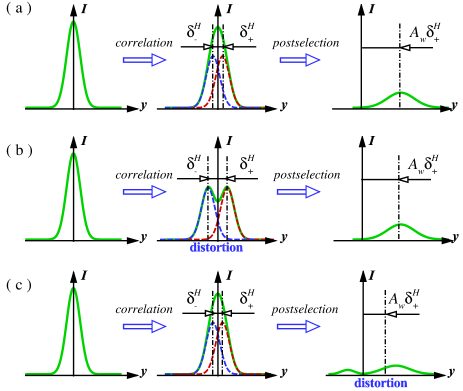
Figure 1: (Color online) Schematic of quantum measurements with preselected and postselected ensembles when probe wavefunction is undisturbed (a) or distorted (b) and (c). System is preselected an initial state $|\psi_{i}\rangle$ and its wavefunction exhibits a Gaussian profile. After weak coupling with the system, the wavefunction splits into two spin components(red dotted line and blue dotted line, respectively). ${+}\delta$ and ${-}\delta$ represent the transverse shifts of left- and right-circularly polarized components, respectively. Then we get the final pointer position proportional to $A_{w}\delta$ after postselection. The green solid lines indicate the total wave shapes. (a) The profile of wavefunction is always Gaussian in the procedure of weak measurement. The conventional weak measurements are valid in this case. (b) The profile of probe wavefunction is distorted in strong coupling, where the displacement exhibits a magnitude on the order of the beam width $\delta\approx{w}$. (c) The other case of the distortion of the probe wavefunction. It occurs when the preselected and postselected states are nearly orthogonal. The conventional weak measurements are invalid and the modified theory should be developed in the latter two cases.

We now consider the preselected state of $|V\rangle$. In a similar way we get the same weak value of the observable $A_{w}$. So we have the amplified factor of the initial state $|V\rangle$ as

$$A_{w}^{V_{con}}=A_{w}^{H_{con}}=F|A_{w}|=\frac{z}{z_{r}}\cot\Delta.$$ (17)

In this case, the original transverse shift is Qin2009

$$\delta^{V}=\frac{(r_{p}+r_{s})\cot\theta_{i}}{k_{0}r_{s}},$$ (18)

and the final amplified shift after free propagation is obtained as

$$A_{w}^{V_{con}}\delta^{V}=\frac{z(r_{p}+r_{s})\cot\theta_{i}\cot\Delta}{z_{r}k_{0}r_{s}}.$$ (19)

From the above analysis, it should be noted that the conditions to obtain the weak value of conventional formalism are too strict. In the experiment of the photonic SHE, if preselected and postselected states are nearly orthogonal, indicating $\langle\psi_{f}|\psi_{i}\rangle\rightarrow 0$, the $A_{w}$ is very large. Thus, the approximations in Eq. (7) is invalid: $[1-ik_{y}\delta^{H,V}A_{w}]\nthickapprox e^{-ik_{y}\delta^{H,V}A_{w}}$. On the other hand, supposing that the preselected state $|H\rangle$ is incident near the Brewster angle, the operator $\exp(-ik_{y}\hat{A}\delta^{H})$ cannot be expanded as $1-ik_{y}\hat{A}\delta^{H}$ due to the strong coupling Luo2011II ; Kong2012 ; Pan2013 ; Gotte2013 . Therefore, the weak value $A_{w}$ in Eq. (7) is inaccurate if one of the conditions is not satisfied. In fact, the two approximations above require the restriction $\delta^{H,V}\cot\Delta\ll w$ from Eq. (15).

We next calculate the final state of the meter in Eq. (7) to second order:

$$|\phiup^{{}^{\prime}}\rangle =\langle\psi_{f}|\psiup^{{}^{\prime}}\rangle$$

$$=\langle\psi_{f}|\left\{\int dk_{y}\phiup(k_{y})|k_{y}\rangle\left(1-ik_{y}\delta\hat{A}-\frac{k_{y}^{2}\delta^{2}}{2}\hat{A}^{2}+\cdots\right)|\psi_{i}\rangle\ \right\}$$

$$\approx\langle\psi_{f}|\psi_{i}\rangle\int dk_{y}\phiup(k_{y})|k_{y}\rangle\left(1-ik_{y}\delta A_{w}-\frac{k_{y}^{2}\delta^{2}}{2}A_{w}^{2}\right),$$ (20)

where $A_{w}^{2}=\frac{\langle\psi_{f}|\hat{A}^{2}|\psi_{i}\rangle}{\langle\psi_{f}|\psi_{i}\rangle}$ is the second-order weak value and $\delta$ is the transverse shift $\delta^{H}$ or $\delta^{V}$. The expectation value of the position is written as

$$\langle y\rangle =\frac{\langle\phiup^{{}^{\prime}}|y|\phiup^{{}^{\prime}}\rangle}{\langle\phiup^{{}^{\prime}}|\phiup^{{}^{\prime}}\rangle}$$

$$=-\frac{2w^{2}\delta(2w^{2}+\delta^{2})\mathrm{Re}(A_{w})}{4w^{2}+3\delta^{4}+4w^{2}\delta^{2}(|A_{w}|^{2}-1)},$$ (21)

with the property $\hat{A}^{2}=1$. Here, the $A_{w}$ is imaginary and therefore we consider the particular form of $\phiup(k_{y})$ with the effective propagation distance $z$: $\phiup(k_{y})\rightarrow\phiup_{z}(k_{y})=\phiup(k_{y})\mathrm{exp}\left(-i\frac{k_{y}^{2}}{2k_{0}}z\right)$ Hosten2008 . Then we can recalculate the position of second-order theory as

$$\langle y\rangle_{2nd}=\frac{4z\delta(3\delta^{2}-2w^{2})|A_{w}|}{k_{0}(4w^{4}+3\delta^{4}+4w^{2}\delta^{2}(|A_{w}|^{2}-1))}.$$ (22)

In the following, we consider the modified theory without approximation. The measuring procedure with preselected and postselected ensembles is still effective in the modified weak measurements. For the preselected state $|H\rangle$, the wave vector $k_{x}$ should be reconsidered when the wave packet incident near the Brewster angle. The evolution in the state after reflection can be written as

$$|k_{x,y}\rangle|H\rangle \rightarrow|k_{x,y}\rangle|\varphi\rangle$$

$$=|k_{x,y}\rangle\left[\left(r_{p}-\frac{k_{x}}{k_{0}}\chi\right)|H\rangle-k_{y}r_{p}\delta^{H}|V\rangle\right]$$

$$=|k_{x,y}\rangle\sum\limits_{+,-}\frac{1}{{\sqrt{2}}}\left(r_{p}-\frac{k_{x}}{k_{0}}\chi\pm ik_{y}r_{p}\delta^{H}\right)|\pm\rangle$$

$$\rightarrow|y\rangle\sum\limits_{+,-}(y\mp\delta^{H_{mod}})|\pm\rangle,$$ (23)

where $\delta^{H_{mod}}$ is defined as the original transverse shift and is given by

$$\delta^{H_{mod}}=\frac{2r_{p}z_{r}(r_{p}+r_{s})\cot\theta_{i}}{2k_{0}r_{p}^{2}z_{r}+\chi^{2}},$$ (24)

and $\chi=\partial r_{p}/\partial\theta_{i}$. So the meter state can be described as

$$|\psiup^{{}^{\prime}}\rangle=\int dk_{x}dk_{y}\phiup_{z}(k_{x,y})|k_{x,y}\rangle|\varphi\rangle.$$ (25)

Subsequently, combine Eq. (11) with Eq. (25), the final meter state becomes

$$|\phiup^{{}^{\prime}}\rangle =\langle\psi_{f}|\psiup^{{}^{\prime}}\rangle$$

$$=\int dk_{x}dk_{y}\phiup_{z}(k_{x,y})|k_{x,y}\rangle\left[\left(\frac{k_{x}}{k_{0}}\chi-r_{p}\right)\sin{\Delta}-k_{y}r_{p}\delta^{H}\cos{\Delta}\right].$$ (26)

The expectation value of the pointer observable $y$, also referred to as modified amplified shift, is obtained as

$$\langle y^{H}\rangle =A_{w}^{H_{mod}}\delta^{H_{mod}}=\frac{\langle\phiup^{{}^{\prime}}|y|\phiup^{{}^{\prime}}\rangle}{\langle\phiup^{{}^{\prime}}|\phiup^{{}^{\prime}}\rangle}$$

$$=\frac{z[2k_{0}r_{p}z_{r}(r_{p}+r_{s})+\chi^{2}]\sin(2\Delta)\cot\theta_{i}}{2k_{0}z_{r}(r_{p}+r_{s})^{2}\cos^{2}\Delta\cot^{2}\theta_{i}+4k_{0}^{2}r_{p}^{2}z_{r}^{2}\sin^{2}\Delta}.$$ (27)

As the preselected state $|V\rangle$, because the coupling is always weak, it still becomes

$$|k_{y}\rangle|V\rangle \rightarrow|k_{y}\rangle(|V\rangle+k_{y}\delta^{V}|H\rangle)$$

$$=|k_{y}\rangle[\exp(+ik_{y}\delta^{V})|+\rangle+\exp(-ik_{y}\delta^{V})|-\rangle]/{\sqrt{2}}.$$ (28)

With the similar calculation in Eqs. (25)-(27), we get the $\langle y^{V}\rangle$ as

$$A_{w}^{V_{mod}}\delta^{V}=\frac{zr_{s}(r_{p}+r_{s})\sin(2\Delta)\cot\theta_{i}}{(r_{p}+r_{s})^{2}\cos^{2}\Delta\cot^{2}\theta_{i}+2k_{0}r_{s}^{2}z_{r}\sin^{2}\Delta}.$$ (29)

Here, $A_{w}^{H_{mod}}$ and $A_{w}^{V_{mod}}$ are the modified amplified factors of states $|H\rangle$ and $|V\rangle$, respectively. Equations (27) and  (29) imply that the theoretical output value is no longer proportional to the weak value, which is different from the conventional theory. But it is worth remarking that the results of the modified theory can reduce to the conventional results as if the condition of weak coupling is satisfied.

For the preselected state $|V\rangle$, when the postselected angle $\Delta$ is not too small, the term $(r_{p}+r_{s})^{2}\cos^{2}\Delta\cot^{2}\theta_{i}$ in Eq. (29) can be ignorable, and Eq. (29) returns to Eq. (19). But for the case of $|H\rangle$, except for the postselected angle limit, the neglect of the term $2k_{0}z_{r}(r_{p}+r_{s})^{2}\cos^{2}\Delta\cot^{2}\theta_{i}$ in Eq. (27) requires that the incident angle is far from the Brewster angle. As a result, Eq. (27) can be reduced to Eq. (16) (under such condition, the $\chi$ can be ignorable). Similarly, such analysis also holds for simplifying the amplified factors of the two different theories. Additionally, we point out that the modified weak measurements are also needed for detecting the photonic SHE with an arbitrary linearly polarized state.

If the condition of weak coupling is satisfied, a weak measurement of the photonic SHE performs as Fig. 1(a). The distribution of the wavefunction is always the Gaussian shape during the procedure of weak measurement. Now we consider the preselected state is $|H\rangle$ with incident angle near the Brewster angle. The separation between two spin components becomes large, which causes the distortion of the wavefunction [ Fig. 1(b)]. On the other hand, in Fig. 1(c), when the preselected and postselected states are nearly or exactly orthogonal, the distortion also occurs after postselection. The distortion of the prove wavefunction accompanies the violation of the limited condition because in the conventional theory where the weak value is calculated under the assumption that wavefunction remains Gaussian. Hence, if the distortion occurs, the quantum system is in the regime where at least one of the two conditions above is violated, and the conventional theory is invalid. To verify it, we measure the intensity of the beam in our weak measurement for some special cases. Our experimental results are also compared with the conventional theory during the discussion. The modified theory is valid not only in weak-coupling regime but also in the strong-coupling regime, and especially in the intermediate regime.

III Experimental results and discussions

To perform the weak measurements of the photonic SHE, the coordinate frame and the experimental setup are similar to that in Ref. Luo2011II . A incident Gauss beam is generated by a He-Ne laser. The two nearly crossed polarizers are used to select the initial state $|\psi_{i}\rangle$ and final state $|\psi_{f}\rangle$. In the experiment, we chose the preselected state as $|H\rangle$ or $|V\rangle$, and the corresponding postselected state is $|V+\Delta\rangle$ or $|H+\Delta\rangle$. The two lenses are used to focus and collimate the beam. When the light beam impinges on air-glass interface, the tiny spin-dependent splitting takes place. After the light passes through the second lens, the amplified shift is detected by a charge-coupled device (CCD).

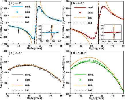
Figure 2: (Color online) Amplified shifts vary with incidence angles. (a) and (b) show the amplified shifts for preselected state $|H\rangle$ with the fixed postselected angles $\Delta$=$2^{\circ}$ and $1^{\circ}$, respectively. (c) and (d) are the cases of $|V\rangle$ with $\Delta=1^{\circ}$ and $0.5^{\circ}$, respectively. The solid lines are the modified values by Eqs. (27) and  (29). In contrast, the long-dashed lines are the predictions of conventional theory by Eqs. (16) and  (19), which have no upper bound for preselected state $|H\rangle$ near the Brewster angle. And the short-dashed lines are the result of second-order theory from Eq. (22). Insets in (a) and (b) show the difference of the three theories in strong-coupling regime. The experimental data represented by hollow points are also given. The arrows in the Fig. 2(a) indicate the two cases in which we measure output intensity of the light beams in Fig. 4.

We first consider the condition of weak coupling. With a fixed preselected angle, the coupling strength varies with incident angles. And then, with the invariable coupling strength, we analyze the other case where the preselected and postselected states are nearly orthogonal. That is, the incident angle is fixed and the outcome is shown as a function of postselected angles. We now experimentally measure the amplified shift, amplified factor, and original displacement of the left-circularly polarized component. We measure the amplified shifts in the case of incident angles varying from $30^{\circ}$ to $80^{\circ}$, as shown in Fig. 2. In each case, the experimental results are also given and agree well with the theoretical curves of modified values. For comparison, the conventional and second-order theories are shown as dashed lines. For the preselected state $|H\rangle$ [Figs. 2(a) and  2(b)], the conventional values are close to the modified values under the condition that the incident angles are far from the Brewster angle. But for the incident angles near the Brewster angle, due to the enhancement of spin-orbit interaction, the splitting of two spin components is nearly the same scale as the width of the Gaussian beam. It means that the weak-coupling condition is violated and the Gaussian profile of wavefunction is distorted. Remarkably, in the strong-coupling regime, the second-order theory also exhibits large distinction with the modified theory.

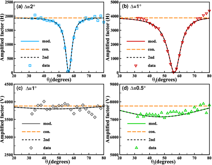
Figure 3: (Color online) Amplified factors vary with incidence angles. (a) and (b) show the cases of preselected state $|H\rangle$. (c) and (d) are the preselected state $|V\rangle$. For all panels, the long- and short-dashed curves are the conventional and second-order theory from Eqs. (17) and Eqs. (22), respectively. The solid curves are modified values from Eqs. (27) and  (29). The experimental data are represented by hollow points.

It is interesting note that for different postselected angles, the divergence between the conventional and modified theories is also different. It indicates that the condition of postselected angle is also important in the weak measurements as well as the weak-coupling condition. In the case of preselected state $|V\rangle$ with the certain angle $\Delta$, the amplifying shift varies with incident angles as shown in Fig. 2(c), both the modified values and the conventional values agree well with the experimental results. Because there is not special angle like the Brewster angle for preselected state $|V\rangle$, the interaction between the observable and the probe state is so weak that the weak-coupling condition is always satisfied. Therefore, as long as the angles $\Delta$ are not too small, the conventional theory can be approximatively equivalent to the modified theory. Otherwise, the two theories diverge and there is almost no overlap between the modified and conventional curves as shown in Fig. 2(d).

Figure 4: (Color online) Distortion of wavefunction due to the strong coupling. The initial state is preselected as $|H\rangle$, the incident angles as $\theta_{i}=40^{\circ}$, and $\theta_{i}=55^{\circ}$, respectively. In addition, the postselected angles are both chosen as $\Delta=2^{\circ}$. (a) and (c) are the theoretical prediction. (b) and (d) are the experimental results. The insets indicate the intensity profiles along the $y$-axis. Note that, in the regime of strong coupling $\theta_{i}=55^{\circ}$, the Gaussian profile of wavefunction distorts and exhibits asymmetric double-peak. But the wavefunction still remains Gaussian form with $\theta_{i}=40^{\circ}$.

To discuss the problem in detail, the corresponding amplified factors shown in Fig. 3 are also given. Generally, according to Eq. (17), the amplified factor of the weak measurements is a constant if the postselected angle $\Delta$ is decided (the straight dashed lines). It is valid if two limited conditions are all satisfied. But the modified amplified factors $A_{w}^{H_{mod}}$ and $A_{w}^{V_{mod}}$ from Eqs. (27) and  (29) are not constants which are shown as solid curves, which are identical to the curves of second-order theory. For state $|H\rangle$, the amplified factor of the modified theory is consistent with that in conventional theory when the incident angles are far away from the Brewster angle, but it becomes small near the Brewster angle. As a result, the largest divergence between modified and conventional values occurs. Comparing Fig. 3(a) with Fig. 3(b), we find that the postselected angle has also important impact on the deviation of the two theories. As predicted, the modified cures coincide well with our experimental data in the strong-coupling regime. For the preselected state $|V\rangle$, we only concern on the limit of postselected angle. In Fig. 3(c), the conventional amplified factor approach to the modified one when the angle $\Delta$ is chosen as $1^{\circ}$. But at first glance, one may regard that there exists discrepancy between the theory and measured data. As a matter of fact, such deviation is appropriate because in this panel the spacing of $y$-axis is suitably small in order to present the divergence of the two theories. Figure 3(d) shows the distinction between the two theories with the $\Delta=0.5^{\circ}$ which is small enough, while our experimental results guarantee the validity of the modified theory.

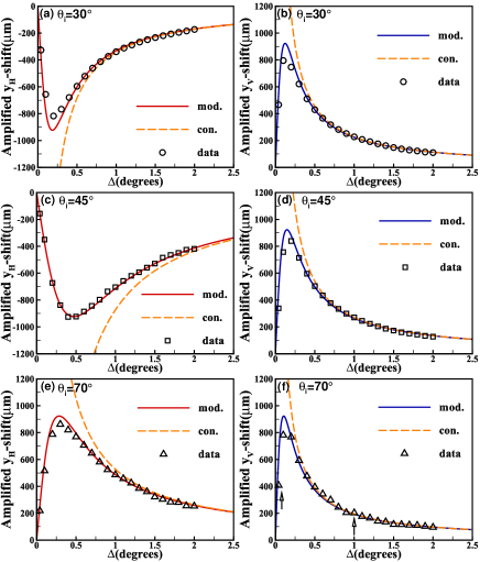
Figure 5: (Color online) With the fixed incident angles $\theta_{i}=30^{\circ}$, $45^{\circ}$, and $70^{\circ}$, amplified pointer shifts are shown as functions of postselected angle $\Delta$ for preselected states $|H\rangle$ (left column) and $|V\rangle$ (right column). Here, the modified theoretical values are represented by solid lines from Eqs. (27) and  (29), and the values in conventional theory are dashed lines from Eqs. (16) and  (19). The sharp value of the dashed lines is not shown in each panel due to its infiniteness. The experimental data are obtained as hollow points. The arrows in the Fig. 5(f) are two special cases in which we measure their output intensity shown in Fig. 7.

If the profile of Gaussian wavefunction is distorted, the theory of weak measurements should be modified. There are two possible cases leading to the distortion in the process of measurements: one is due to the strong coupling, the other to the preselected and postselected states are nearly orthogonal. We first consider the former case. The initial state is preselected as $|H\rangle$ as shown in Fig. 4, which explains the connection between distortion of the beam and the weak-interaction condition. To avoid the limited condition of postselected angle, we set it to be $\Delta=2^{\circ}$. We consider two special examples labeled by arrows in Fig. 2(a). The measured intensity is read out from CCD (right column of Fig. 4). For comparison, the corresponding predictions are also given (left column of Fig. 4). The case with incident angle $\theta_{i}=40^{\circ}$ suggests that the conventional theory is equivalent to the modified one if the output beam remains the Gaussian profile. Conversely, at the incident angle $55^{\circ}$ the wavefunction distorts due to the strong coupling and the conventional theory of weak measurements is invalid.

Figure 6: (Color online) Amplified factors with various postselected angle. (a), (c), and (e) show the cases of $|H\rangle$. (b), (d), and (f) are $|V\rangle$. In term of Eqs. (17),  (27), and  (29), the predictions of the modified and conventional theory are represented by solid lines and dashed lines, respectively. The conventional amplified factor can be arbitrarily large with the angle $\Delta$ decreasing to $0^{\circ}$. The hollow points are experimental data.

All discussion above is about the weak-interaction condition in the modified weak measurements. In the rest of the paper, we consider another limited condition of small postselected angle, that is to say the preselected and postselected states are nearly orthogonal. We find that the weak measurements of conventional theory are also not valid when the postselected angle $\Delta$ is too small. To prove that, we detect the photonic SHE with the fixed incident angles but various postselected angles. In the same sequence, we first measure the amplified shifts with the angle $\Delta$ varying from $0^{\circ}$ to $2.5^{\circ}$, which are shown in Fig. 5. Under such condition, large divergence takes place between modified and conventional theories when the angle $\Delta$ is close to $0^{\circ}$. But the amplified values in conventional theory essentially have no difference to that in modified theory with appropriate postselected angles. In the conventional theory of the weak measurements, according to the Eqs. (16) and  (19), the amplified value can be arbitrarily large if the preselected and postselected states are nearly crossed, and such value is shown as the dashed lines in the figures.

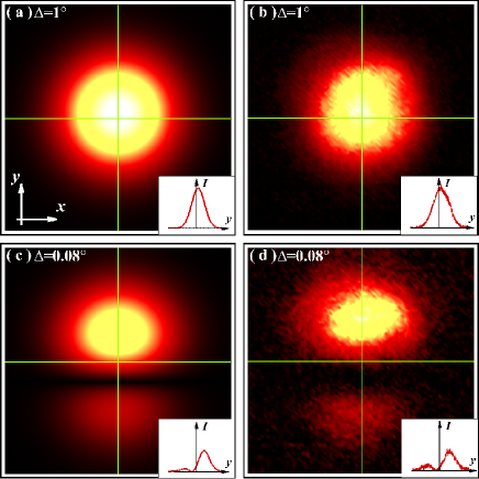
Figure 7: (Color online) Distortion of probe wavefunction due to the fact that the preselected and postselected states are nearly orthogonal. We chose the preselected state as $|V\rangle$ with a fixed incident angle at $\theta_{i}=70^{\circ}$. (a) and (c) are the theoretical results. (b) and (d) are the experimental results. The insets: the profiles of wavefunction at the plane of $x=0$. It implies that the output wavefunction no longer remains a Gaussian profile when the preselected and postselected states are nearly orthogonal.

Whereas in our modified theory (the solid lines), with the angle $\Delta$ continuously decreasing to $0^{\circ}$, the amplified shift first increases and reaches the maximum value, then decreases rapidly even to $0^{\circ}$. We do the experiment with the incident angles $\theta_{i}=30^{\circ}$, $45^{\circ}$, and $70^{\circ}$ both for states $|H\rangle$ and $|V\rangle$, and our experimental data reveal the trend like the modified theory. Note that in Fig. 5(c), the modified and conventional curves begin to separate when the $\Delta$ is near $2.5^{\circ}$, but in other cases, such separation takes place until the $\Delta$ becomes smaller. The point is that in this case the weak-interaction is a little strong at the incident angle $\theta_{i}=45^{\circ}$. To clarify it, we see that the example in Fig. 5(d), with the same incident angle but different preselected state $|V\rangle$, dose not exist such problem. We point out that when the postselected angles are negative, the values of amplified shift are the same magnitude but opposite sign, besides, the amplified shift of second-order theory is completely identical to the modified one, which both are not shown here.

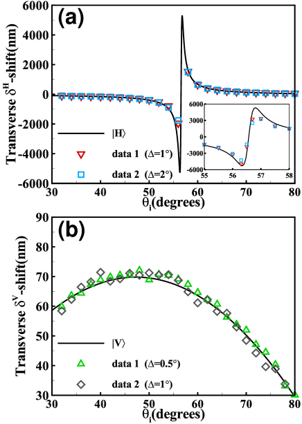
Figure 8: (Color online) Original transverse shifts of the spin component $|+\rangle$ for preselected states: (a) $|H\rangle$ and (b) $|V\rangle$. The theoretical values are represented by black solid lines from Eqs. (18) and  (24). For each preselected state, the experiment data with two different postselected angles $\Delta$ are shown as hollow points. Inset in (a) shows the theoretical and experimental results in strong-coupling regime.

In addition, the corresponding amplified factors are also obtained in Fig. 6. We get the conventional amplified factors represented by dashed lines in terms of the relation $A_{w}^{H_{con}}=A_{w}^{V_{con}}=F|A_{w}|$. It is shown that the amplified factor has no upper bound when the $\Delta$ approaches to $0^{\circ}$. In fact, both for two preselected states $|H\rangle$ and $|V\rangle$, the behavior of the amplified factors $A_{w}^{H_{mod}}$ and $A_{w}^{V_{mod}}$ shown as the solid lines is similar to that of amplified shifts. In each panel, the modified theory is compared with the conventional theory, and once again, the difference between conventional and modified values would be significant if the preselected angle $\Delta$ is small. The deviation of the amplified factors between the two theories is also determined by incident angle, especially for $|H\rangle$. The experimental results agree well with the modified values. There exists a peak value with an optimal postselected angle, and the amplification effect disappears when the preselected and postselected states are completely orthogonal. That is to say, by adjusting the postselected angle $\Delta$, one can obtain the maximum amplified factor and improve the precision for measuring the photonic SHE Zhou2014I ; Zhou2014II . Note that the signal amplification from weak measurements has been extensively studied recently, such as optimal probe wavefunction of weak-value amplification Susa2012 , technical advantages for weak-value amplification Jordan2014 , and maximizing the output by weak values and weak coupling Lorenzo2014 . Note that there are still some open questions about whether the weak value ampliation can suppress technical noise Knee2014 ; Ferrie2014 .

We have discussed the connection between the condition of weak-interaction and the output intensity of the light in Fig. 4. Here, we analyze the distortion associated with the postselected angle. In the case of Fig. 5(f), we measured its intensity with a decreasing angle $\Delta$, and found that the intensity changes gradually from a single Gaussian into asymmetrical double-peak intensity. Then the double-peak intensity becomes symmetric when postselected angle is equal to $0^{\circ}$. In particular, in Fig. 7, we present the intensity with two postselected angles which are labeled by the arrows in Fig. 5(f). Both for the predicted and measured intensity, they remain the Gaussian form with the $\Delta=1^{\circ}$, but distort with the $\Delta=0.08^{\circ}$. We draw a conclusion that with different postselected angles, the experimental data do not fit to the conventional theory when the profile of wavefunction distorts. Therefore, one may judge weather the modified theory is equivalent to the conventional one by observing the output intensity of the light.

The tiny original shifts of the component of $|+\rangle$ obtained by the modified theory for preselected states $|H\rangle$ and $|V\rangle$ are presented in Fig. 8. For each preselected states, we detect it with two different postselected angles. We find that the original shift of $|H\rangle$ is indeed very large near the Brewster angle: nearly the same scale as the width of probe state $|{\delta^{H}}|\approx{w}$, As the result, the profile is strongly distorted and the weak measurements approximations fail. For the preselected state $|V\rangle$, the original shifts for various incident angles are always much less than the width of pointer state $|{\delta^{V}}|\ll{w}$. Both experimental results agree well with the theoretical predictions.

It should be noted in the strong-coupling case the spin-dependent splitting is very sensitive to the variation of physical parameters and therefore has important applications in precision metrology, such as measuring thickness of metal film Zhou2012I , identifying graphene layers Zhou2012II , determining the strength of axion coupling in topological insulators Zhou2013 , and detecting of magneto-optical constant of magneto-optical media Qiu2014 . However, in this regime both conventional weak measurements theory and its second-order corrections cannot obtain the exact meter shifts as the analysis above. Hence the modified weak measurement is important in precision metrology.

Finally, it should be mentioned that photonic SHE manifests as spin-dependent splitting of light, which corresponds to two types of geometric phases: the Rytov-Vladimirskii-Berry phase associated with the evolution of the propagation direction of light and the Pancharatnam-Berry phase related to the manipulation with the polarization state of light Bliokh2008I . In general, the spin-dependent splitting due to the Rytov-Vladimirskii-Berry phase is limited by a fraction of the wavelength, and can only be detected by weak measurements Hosten2008 . However, the spin-dependent splitting due to the Pancharatnam-Berry phase can be large enough for direct detection (strong measurements) without using the weak measurement technology Bliokh2008II ; Gorodetski2008 ; Shitrit2011 ; Shitrit2013 ; Ling2014 ; Ling2015 . In addition, the rapidly varying phase discontinuities along a metasurface, breaking the axial symmetry of the system, enable the direct observation of the spin-dependent splitting Yin2013 . In the intermediate regime, the modified theory is important where neither weak nor strong measurements can detect the spin-dependent splitting.

IV Conclusions

In conclusion, we have developed a modified weak measurements for the detection of the photonic SHE. Compared with the conventional weak measurements, the amplified shift, amplified factor, and original displacement for different preselected and postselected states have been examined. The conventional theory for preselected state $|H\rangle$ is invalid in the strong-coupling regime or when the preselected and postselected states are nearly orthogonal. But for preselected state $|V\rangle$ it is only limited by the latter since the condition of weak coupling is always satisfied. We have shown that the weak measurements for detecting photonic SHE need to be modified when one of the condition is violated. This is due to the fact that probe wavefunction is distorted in the case of strong coupling or preselected and postselected states are nearly orthogonal. Otherwise, the modified theory can reduce to the conventional one beyond the two restrictions. We have found that the measuring procedure with preselected and postselected ensembles is still effective. This scheme is important for us to detect the photonic SHE in the case where neither weak nor strong measurements can detect the spin-dependent splitting. Our modified theory is valid not only in weak-coupling regime but also in the strong-coupling regime, and especially in the intermediate regime. We believe that such problem may also exist in the weak measurements of other quantum systems and would have possible applications in precision measurements.

- (1) Y. Aharonov, D. Z. Albert, and L. Vaidman, Phys. Rev. Lett. 60, 1351 (1988).
- (2) I. M. Duck, P. M. Stevenson, and E. C. G. Sudarshan, Phys. Rev. D 40, 2112 (1989).
- (3) N. W. M. Ritchie, J. G. Story, and R. G. Hulet, Phys. Rev. Lett. 66, 1107 (1991).
- (4) A. D. Parks, D. W. Cullin, and D. C. Stoudt, Proc. R. Soc. Lond. 454, 2997 (1998).
- (5) A. M. Steinberg, P. G. Kwiat, and R. Y. Chiao, Phys. Rev. Lett. 71, 708 (1993).
- (6) P. B. Dixon, D. J. Starling, A. N. Jordan, and J. C. Howell, Phys. Rev. Lett. 102, 173601 (2009).
- (7) N. Brunner and C. Simon, Phys. Rev. Lett. 105, 010405 (2010).
- (8) D. J. Starling, P. B. Dixon, A. N. Jordan, and J. C. Howell, Phys. Rev. A 82, 063822 (2010).
- (9) A. Feizpour, X. Xing, and A. M. Steinberg, Phys. Rev. Lett. 107, 133603 (2011).
- (10) X.-Y. Xu, Y. Kedem, K. Sun, L. Vaidman, C.-F. Li, and G.-C. Guo, Phys. Rev. Lett. 111, 033604 (2013).
- (11) O. S. Magaña-Loaiza, M. Mirhosseini, B. Rodenburg, and R. W. Boyd, Phys. Rev. Lett. 112, 200401 (2014).
- (12) G. J. Pryde, J. L. O'Brien, A. G. White, T. C. Ralph, and H. M. Wiseman, Phys. Rev. Lett. 94, 220405 (2005).
- (13) J. S. Lundeen and A. M. Steinberg, Phys. Rev. Lett. 102, 020404 (2009).
- (14) S. Kocsis, B. Braverman, S. Ravets, M. J. Stevens, R. P. Mirin, L. K. Shalm, and A. M. Steinberg, Science 332, 1170 (2011).
- (15) L. A. Rozema, A. Darabi, D. H. Mahler, A. Hayat, Y. Soudagar, and A. M. Steinberg, Phys. Rev. Lett. 109, 100404 (2012).
- (16) J. Z. Salvail, M. Agnew, A. S. Johnson, E. Bolduc, J. Leach, and R.W. Boyd, Nat. Photonics 7, 316 (2013).
- (17) J. S. Lundeen, B. Sutherland, A. Patel, C. Stewart, and C. Bamber, Nature 474, 188 (2011).
- (18) M. Mirhosseini, O. S. Magaña-Loaiza, S. M. H. Rafsanjani, and R. W. Boyd, Phys. Rev. Lett. 113, 090402 (2014).
- (19) M. Malik, M. Mirhosseini, M. P. J. Lavery, J. Leach, M. J. Padgett, and R. W. Boyd, Nat. Commun. 5, 4115 (2014).
- (20) Y. Aharonov, S. Popescu, D. Rohrlich, and P. Skrzypczyk, New J. Phys. 15, 113015 (2013).
- (21) T. Denkmayr, H. Geppert, S. Sponar, H. Lemmel, A. Matzkin, J. Tollaksen, and Y. Hasegawa, Nat. Commun. 5, 4492 (2014).
- (22) O. Hosten and P. Kwiat, Science 319, 787 (2008).
- (23) M. Onoda, S. Murakami, and N. Nagaosa, Phys. Rev. Lett. 93, 083901 (2004).
- (24) K. Y. Bliokh and Y. P. Bliokh, Phys. Rev. Lett. 96, 073903 (2006).
- (25) C. M. Krowne, Phys. Lett. A 373, 466 (2009).
- (26) S. Wu and Y. Li, Phys. Rev. A 83, 052106 (2011).
- (27) X. Zhu, Y. Zhang, S. Pang, C. Qiao, Q. Liu, and S. Wu, Phys. Rev. A 84, 052111 (2011).
- (28) T. Koike and S. Tanaka, Phys. Rev. A 84, 062106 (2011).
- (29) J. Dressel and A. N. Jordan, Phys. Rev. Lett. 109, 230402 (2012).
- (30) A. Di Lorenzo, Phys. Rev. A 85, 032106 (2012).
- (31) A. K. Pan and A. Matzkin, Phys. Rev. A 85, 022122 (2012).
- (32) T. Geszti, Phys. Rev. A 81, 044102 (2010).
- (33) K. Nakamura, A. Nishizawa, and M.-K. Fujimoto, Phys. Rev. A 85, 012113 (2012).
- (34) S. Pang, S. Wu, and Z.-B. Chen, Phys. Rev. A 86, 022112 (2012).
- (35) A. G. Kofman, S. Ashhab, and F. Nori, Phys. Rep. 520, 43 (2012).
- (36) H. Luo, X. Ling, X. Zhou, W. Shu, S. Wen, and D. Fan, Phys. Rev. A 84, 033801 (2011).
- (37) J. Dressel, M. Malik, F. M. Miatto, A. N. Jordan, and R.W. Boyd, Rev. Mod. Phys. 86, 307 (2014).
- (38) Y. Gorodetski, K. Y. Bliokh, B. Stein, C. Genet, N. Shitrit, V. Kleiner, E. Hasman, and T.W. Ebbesen, Phys. Rev. Lett. 109, 013901 (2013).
- (39) J. Dressel and A. N. Jordan, Phys. Rev. A 85, 012107 (2012).
- (40) Y. Aharonov, A. Botero, S. Popescu, B. Reznik, and J. Tollaksen, Phys. Lett. A 301, 130 (2002).
- (41) R. Jozsa, Phys. Rev. A 76, 044103 (2007).
- (42) N. S. Williams and A. N. Jordan, Phys. Rev. Lett. 100, 026804 (2008).
- (43) A. Romito, Y. Gefen, and Y. M. Blanter, Phys. Rev. Lett. 100, 056801 (2008).
- (44) H. Kobayashi, G. Puentes, and Y. Shikano, Phys. Rev. A 86, 053805 (2012).
- (45) A. Aiello and J. P. Woerdman, Opt. Lett. 33, 1437 (2008).
- (46) Y. Qin, Y. Li, H. He, and Q. Gong, Opt. Lett. 34, 2551 (2009).
- (47) H. Luo, X. Zhou, W. Shu, S. Wen, and D. Fan, Phys. Rev. A 84, 043806 (2011).
- (48) L. J. Kong, X. L. Wang, S. M. Li, Y. N. Li, J. Chen, B. Gu, and H. T. Wang, Appl. Phys. Lett. 100, 071109 (2012).
- (49) M.-M. Pan, Y. Li, J.-L. Ren, B. Wang, Y.-F. Xiao, H. Yang, and Q. Gong, App. Phys. Lett. 104, 051130 (2013).
- (50) J. B. Götte and M. R. Dennis, Opt. Lett. 38, 2295 (2013).
- (51) X. Zhou, X. Li, H. Luo, and S. Wen, App. Phys. Lett. 104, 051130 (2014).
- (52) X. Zhou, X. Ling, Z. Zhang, H. Luo, and S. Wen, Sci. Rep. 4, 7388 (2014).
- (53) Y. Susa, Y. Shikano, and A. Hosoya, Phys. Rev. A 85, 052110 (2012).
- (54) A. N. Jordan, J. Martínez-Rincón, and J. C. Howell, Phys. Rev. X 4, 011031 (2014).
- (55) A. D. Lorenzo, Ann. Phys. 345, 178 (2014).
- (56) G. C. Knee and E. M. Gauger, Phys. Rev. X 4, 011032 (2014).
- (57) C. Ferrie and J. Combes, Phys. Rev. Lett. 112, 040406 (2014).
- (58) X. Zhou, Z. Xiao, H. Luo, and S. Wen, Phys. Rev. A 85, 043809 (2012).
- (59) X. Zhou, X. Ling, H. Luo, and S. Wen, Appl. Phys. Lett. 101, 251602 (2012).
- (60) X. Zhou, J. Zhang, X. Ling, S. Chen, H. Luo, and S. Wen, Phys. Rev. A 88, 053840 (2013).
- (61) X. Qiu, X. Zhou, D. Hu, J. Du, F. Gao, Z. Zhang, and H. Luo, Appl. Phys. Lett. 105, 131111 (2014).
- (62) K. Y. Bliokh, A. Niv, V. Kleiner, and E. Hasman, Nat. Photonics 2, 748 (2008).
- (63) K. Y. Bliokh, Y. Gorodetski, V. Kleiner, and E. Hasman, Phys. Rev. Lett. 101, 030404 (2008)
- (64) Y. Gorodetski, A. Niv, V. Kleiner, and E. Hasman, Phys. Rev. Lett. 101, 043903 (2008).
- (65) N. Shitrit, I. Bretner, Y. Gorodetski, V. Kleiner, and E. Hasman, Nano Lett. 11, 2038 (2011).
- (66) N. Shitrit, I. Yulevich, E. Maguid, D. Ozeri, D. Veksler, V. Kleiner, and E. Hasman, Science 340, 724 (2013).
- (67) X. Ling, X. Yi, X. Zhou, Y. Liu, W. Shu, H. Luo, and S. Wen, App. Phys. Lett. 105, 151101 (2014).
- (68) X. Ling, X. Zhou, X. Yi, W. Shu, Y. Liu, S. Chen, H. Luo, S. Wen, and D. Fan, Light: Sci. Appl. 4, e290 (2015).
- (69) X. Yin, Z. Ye, J. Rho, Y. Wang, and X. Zhang, Science 339, 1405 (2013).