Fourier analysis of multi-tracer cosmological surveys

Abstract

We present optimal quadratic estimators for the Fourier analysis of cosmological surveys that detect several different types of tracers of large-scale structure. Our estimators can be used to simultaneously fit the matter power spectrum and the biases of the tracers — as well as redshift-space distortions (RSDs), non-Gaussianities (NGs), or any other effects that are manifested through differences between the clusterings of distinct species of tracers. Our estimators reduce to the one by Feldman, Kaiser & Peacock (ApJ 1994, FKP) in the case of a survey consisting of a single species of tracer. We show that the multi-tracer estimators are unbiased, and that their covariance is given by the inverse of the multi-tracer Fisher matrix (Abramo, MNRAS 2013; Abramo & Leonard, MNRAS 2013). When the biases, RSDs and NGs are fixed to their fiducial values, and one is only interested in measuring the underlying power spectrum, our estimators are projected into the estimator found by Percival, Verde & Peacock (MNRAS 2003). We have tested our estimators on simple (lognormal) simulated galaxy maps, and we show that it performs as expected, being equivalent or superior to the FKP method in all cases we analyzed. Finally, we have shown how to extend the multi-tracer technique to include the 1-halo term of the power spectrum.

1 Introduction

Astrophysical surveys have come to occupy a central role in cosmology (York et al., 2000; Cole et al., 2005; Abbott et al., 2005; Scoville et al., 2007; Adelman-McCarthy et al., 2008a, b; PAN-STARRS, ; BOSS, ; Blake et al., 2011). Percent-level accuracies can now be reached on distance measurements at high redshifts, both across and along the line-of-sight (Anderson et al., 2012, 2014). This means more and better constraints on the acceleration of the expansion rate of the Universe, on modified gravity (Linder, 2005), on non-Gaussian initial conditions (Verde et al., 2000; Bartolo et al., 2004), and about the role of massive neutrinos, among other applications.

The groundbreaking achievements of the Sloan Digital Sky Survey (York et al., 2000) are being surpassed by other surveys with higher completeness, wider wavelength coverage, and a larger range of redshifts (BigBOSS, ; SUMIRE, ; Ellis et al., 2012; Abell et al., 2009). Some surveys will specialize in mapping very large volumes to an extremely high completeness, by employing imaging with narrow-band filters (Benítez et al., 2009, 2014), or by resorting to low-resolution integral-field spectroscopy (Hill, 2008). In addition to galaxies, quasars can also serve both as sources of background light to investigate the intervening matter through the Ly-$\alpha$ forest (Slosar et al., 2013), or directly as tracers of the large-scale structure (Croom et al., 2005; da Ângela et al., 2005; Yahata et al., 2005; Shen et al., 2007; Ross et al., 2009; Sawangwit et al., 2012; Abramo et al., 2012; Leistedt et al., 2013; Leistedt & Peiris, 2014). Another way in which the 3D matter distribution can be mapped is through the 21cm hyperfine transition of neutral H, and new radiotelescopes dedicated to measuring that line are being deployed or are in the planning stages (Bandura et al., 2014; Battye et al., 2012).

This intense activity points to an exciting future, where vast volumes of the Universe will be increasingly mapped in a variety of ways, and with different types of tracers of the large-scale structure.

However, these maps are not independent, since all tracers sit on the same distribution of dark matter. This points to a key obstacle on the way to explore the full power of these overlapping surveys: cosmic variance – a particular case of sample variance, where the sample is the set of modes of the density perturbations which were realized in some region of the Universe from a (nearly) Gaussian random process.

Despite this fundamental limitation, it was pointed out by Seljak (2009); McDonald & Seljak (2008) that the bounds imposed by cosmic variance do not apply for many key physical quantities of interest. In particular, by comparing the clustering of tracers with different biases one can measure some parameters to an accuracy which is basically unconstrained by cosmic variance. This applies not only to bias itself, but to the matter growth rate of the RSDs, to the NG parameters $f_{NL}$ and $g_{NL}$, as well as any parameters that affect the relative clusterings of different tracers. The consequences of this extraordinary windfall were explored in many papers – see, e.g., Slosar (2009); Gil-Marín et al. (2010); Cai & Bernstein (2011a, b); Hamaus et al. (2011); Smith, Desjacques & Marian (2011); Hamaus et al. (2012); Abramo & Leonard (2013); Blake et al. (2013); Bull et al. (2014); Ferramacho et al. (2014); Hamaus et al. (2014). It is important to stress that this additional information comes from measuring the two-point functions of the different tracers, as opposed to enhancing the signal-to-noise by employing different statistics such as mass-weighting (Seljak et al., 2009; Cai et al., 2011; Smith & Marian, 2014).

In Abramo & Leonard (2013) we showed that the enhanced constraints of multi-tracer cosmological surveys are a straightforward consequence of the multi-tracer Fisher information matrix (Abramo, 2012). In the presence of $N$ different types of tracers, each one with a different bias, there is a simple choice of variables which diagonalizes the multi-tracer Fisher matrix: in addition to the underlying power spectrum (which is subject to the cosmic variance bounds), there are $N-1$ variables which correspond to the relative clustering strengths between the tracers. These relative clustering strengths are not affected by cosmic variance, and their measurements can be arbitrarily accurate, even if the survey has a finite volume. In the case of a single tracer, the multi-tracer Fisher matrix reduces to the usual case treated in the seminal paper by Feldman et al. (1994) (henceforth FKP).

In this paper we use the multi-tracer Fisher matrix to derive optimal estimators for the redshift-space power spectra of an arbitrary number of different types of tracers of large-scale structure (see Sec. 3). These tracers may overlap in some regions but not others, or not at all. The tracers can be galaxies of different types, quasars, Ly-$\alpha$ absorption systems, etc. One may also choose to trade individual objects by halos of different masses — in which case the bias of the tracers become the halo bias (Seljak et al., 2009; Hamaus et al., 2010; Cai et al., 2011; Smith & Marian, 2014, 2015).

Our formulas can be used in any of those situations, in real or in redshift-space, including effects such as scale-dependent bias. An important cross-check is that a particular combination (or projection) of our estimators leads back to the estimator of Percival et al. (2003) (henceforth PVP), — namely, the PVP estimator follows from ours if the biases of the tracers, as well as the RSDs, are fixed to their true values, and one then computes the underlying matter power spectrum using the aggregated clustering information from all the tracers.

We have also incorporated the contribution of the 1-halo term to the covariance of the galaxy counts (see Sec. 6) into the multi-tracer Fisher matrix. In principle, the full covariance can be computed using the Halo Model (Cooray & Sheth, 2002), together with appropriate halo occupation distributions for the tracers. Recently, Smith & Marian (2015) presented an optimal estimator for the power spectrum including all Halo Model corrections to the spectrum, bispectrum and trispectrum. However, the Smith & Marian (2015) estimator generalizes the estimator of Percival et al. (2003), while we have obtained estimators not only for the matter power spectrum, but also for the biases, RSDs, NGs, etc. Hence, we are only able to include the simplest correction to galaxy clustering from the halo model (the 1-halo term), but our framework allows the simultaneous estimation of bias, RSDs and the power spectrum, while Smith & Marian (2015), include all the corrections that can be computed on the basis of the Halo Model, but their estimator applies only to the power spectrum, and assumes prior knowledge of the bias of all the species, as well as of the shape of the RSDs.

The Fisher matrix and the covariance of the counts of the tracers are the basic objects used to construct our estimators – in fact, the optimal estimators are a type of Wiener filtering, in the sense that we are basically weighting the data by the inverse of their covariance. We employ results and notation introduced in Abramo (2012); Abramo & Leonard (2013), and the construction of the estimators follows the steps outlined in Tegmark (1997); Tegmark et al. (1998).

The estimators were tested using simple mock galaxy catalogs based on lognormal maps (Sec. 5). We find that the empirical covariance of the power spectra is well approximated by the theoretical covariance (the inverse of the multi-tracer Fisher matrix), confirming the optimality of the estimator.

The main formulas of this paper are derived in Sec. 3, and a practical algorithm for the Fourier analysis of multi-tracer surveys is summarized in Sec. 5.2.

This paper is organized as follows: in Sec. 2 we review the Fisher information matrix for single-tracer and multi-tracer cosmological surveys. In Sec. 3 we construct the optimal quadratic estimators on the basis of the covariance matrix for the data. In Sec. 4 we discuss the relationships between the multi-tracer estimators and other methods, such as FKP and PVP, as well as the main features of the multi-tracer technique. In Sec. 5 we test the estimators in simple simulated maps, showing that the empirical covariance matches closely the theoretical covariance — which establishes that the multi-tracer estimators are unbiased and optimal. In Sec. 6 we show how to include the 1-halo term in the estimators of the multi-tracer power spectra. We also show there how to construct estimators for the 1-halo term, and how to generalize the procedure to estimate simultaneously the 2-halo and the 1-halo term of the power spectrum. We conclude in Section 7.

2 The information in galaxy surveys

The matter power spectrum is defined through the expectation value $\langle\delta_{m}(\vec{k},z)\delta_{m}^{*}(\vec{k}^{\prime},z)\rangle=(2\pi)^{3}P_{m}(k,z)\delta_{D}(\vec{k}-\vec{k}^{\prime})$, where $\delta_{m}(\vec{k})$ is the matter density contrast, and $\delta_{D}$ is the Dirac delta function. However, galaxy surveys actually measure counts of tracers of the large-scale structure (galaxies and other extragalactic objects) in redshift space. It is from those observable that we can then measure derived quantities such as the baryon acoustic oscillations (Eisenstein et al., 1999; Blake & Glazebrook, 2003; Seo & Eisenstein, 2003), or the pattern of redshift-space distortions (Kaiser, 1987; Hamilton, 2005a, b).

For a tracer of type $\alpha$, whose counts as a function of (redshift-space) position are $n_{\alpha}(\vec{x})$, the density contrast is $\delta_{\alpha}(\vec{x})=n_{\alpha}(\vec{x})/\bar{n}_{\alpha}(\vec{x})-1$. The mean number densities $\bar{n}_{\alpha}$ should reflect the spatial modulations of the observed numbers of galaxies which are due to the instrument, the strategy and schedule of observations, as well as any other factors unrelated to the redshift-space cosmological fluctuations.

If we assume that bias is linear and deterministic, then in the distant-observer approximation the redshift-space fluctuations in the counts of the $\alpha$-type galaxies are related to the underlying mass fluctuations by the relation $\delta_{\alpha}(\vec{k},z)\simeq[b_{\alpha}+f\,\mu_{k}^{2}]\delta_{m}(\vec{k},z)\,$. Here $b_{\alpha}$ is the bias of the tracer species $\alpha$, $f(z)$ is the matter growth rate, and $\mu_{k}=\hat{k}\cdot\hat{r}$ is the cosine of the angle between the Fourier mode and the line of sight.

The index $\alpha$ (we employ greek letters to denote different tracer species) can be any kind of discriminant of the types of tracers of large-scale structure: it may stand for luminosity, morphological type, star formation rate, equivalent width of some emission line, or a combination of those. One may also regard the dark matter halos themselves as the tracers, in which case $\alpha$ would stand for the halo mass (or some proxy for it, such as richness), and the bias $b_{\alpha}$ becomes halo bias.

There are some complicating factors in this description. First, structure formation should introduce a scale dependence for the bias, as well as some degree of stochasticity (Benson et al., 2000; Dekel & Lahav, 1999; Weinberg, 2002; Smith, Scoccimarro & Sheth, 2009). Second, the initial conditions may contain non-Gaussian features, which would manifest themselves as an additional scale-dependent bias (Bartolo et al., 2004; Sefusatti & Komatsu, 2007; Dalal et al., 2008). Third, the velocity dispersion from random motions inside halos will smear the galaxy density contrast, affecting the shape of RSDs. In fact, the RSD parameters and angular dependence can inherit scale-dependent non-linear corrections (Raccanelli et al., 2012)

Hence, in practice it is more useful to regard “bias” as a more general function of redshift, scale, and angle with the line-of-sight that should be determined by observations, and define the clustering of a species $\alpha$ as:

$$P_{\alpha}\equiv B_{\alpha}^{2}\,P_{m}\;,$$ (1)

where $B_{\alpha}=b_{\alpha}+f\mu_{k}^{2}+\Delta b_{NG}$ is an effective bias. This effective bias can include not only RSDs and non-Gaussianities (NGs), but also scale-dependence of the bias, or any other effect that distorts the power spectrum of the tracers relative to the underlying matter distribution.

In principle, everything depends on $\vec{x}$ and $\vec{k}$, but one can regard $x$ (i.e., the radial position) as standing in for redshift, so we could also write $B_{\alpha}=B_{\alpha}(z,k,\mu_{k})$, and $P_{m}=P_{m}(z,k)$. Since the matter power spectrum, bias, RSDs, as well as NGs and other corrections, are just subproducts of clustering measurements for all the available tracers in a given survey, the problem we must address is how one can optimally estimate the clusterings $P_{\alpha}(\vec{x},\vec{k})$. Our approach also means that cross-correlations are expressed as $P_{\alpha\beta}=B_{\alpha}B_{\beta}P_{m}$.

2.1 Optimal estimators and the Fisher matrix

The Fisher information matrix can be constructed from the data covariance after a series of simple steps – for a review in the specific context of cosmological surveys, see, e.g., Tegmark et al. (1997); Tegmark (1997); Tegmark et al. (1998).

Let’s assume that the measured quantities (the data) are $d_{i}$, such that, for simplicity, their expectation values vanish: $\langle d_{i}\rangle=0$. The data covariance is then $C_{ij}=Cov(d_{i},d_{j})=\langle d_{i}d_{j}\rangle$. From this data we would like to extract some set of parameters $p_{\mu}$, whose likelihoods we assume to be approximately described by a multivariate Gaussian. Under these conditions, the Fisher information matrix is given by:

$$F_{\mu\nu} \equiv F[p_{\mu},p_{\nu}]=-\langle\frac{\partial^{2}\log{\cal{L}}}{\partial p_{\mu}\partial p_{\nu}}\rangle$$

$$\simeq \frac{1}{2}\sum_{ijkl}C_{ij}^{-1}\frac{\partial C_{jk}}{\partial p_{\mu}}C_{kl}^{-1}\frac{\partial C_{li}}{\partial p_{\nu}}\;,$$

$$= \frac{1}{2}\,{\rm Tr}\left[C^{-1}\frac{\partial C}{\partial p_{\mu}}C^{-1}\frac{\partial C}{\partial p_{\nu}}\right]\;,$$

where the second line follows from the assumption of near-Gaussianity of the likelihood near its maximum.

Now suppose that estimators $\hat{p}_{\mu}$ can be constructed, such that their covariance $Cov(\hat{p}_{\mu},\hat{p}_{\nu})=F^{-1}_{\mu\nu}$. These estimators must then be optimal, in the sense that they saturate the Cramér-Rao bound: $Cov(\hat{p}_{\mu},\hat{p}_{\nu})\geq F^{-1}_{\mu\nu}$.

There are in fact such estimators, which can be constructed after a few simple steps, and which employ the same basic objects that appear in the Fisher matrix. The first step is to create the quadratic form:

$$\hat{q}_{\mu}\equiv\sum_{ij}E_{\mu}^{ij}d_{i}d_{j}-\Delta_{\mu}\;,$$ (3)

where

$$E_{\mu}^{ij}=\frac{1}{2}\sum_{kl}C^{-1}_{ik}\frac{\partial C_{kl}}{\partial p_{\mu}}C^{-1}_{lj}.$$ (4)

Here, $\Delta_{\mu}$ serves to subtract any possible bias the estimators may have, such that we end up with unbiased estimators whose expectation values coincide with their fiducial values.

Gaussianity of the data (a key underlying assumption) implies that the 4-point function $\langle d_{i}d_{j}d_{k}d_{l}\rangle=C_{ij}C_{kl}+C_{ik}C_{jl}+C_{il}C_{jk}$, and from it follows, after some algebra, that the covariance of the quadratic form above is $Cov(\hat{q}_{\mu},\hat{q}_{\nu})=F_{\mu\nu}$.

The final step is to define the optimal quadratic estimators in such a way that their covariance is the inverse of the Fisher matrix. Clearly, then, the estimators:

$$\hat{p}_{\mu}=\sum_{\alpha}F^{-1}_{\mu\alpha}\,\hat{q}_{\alpha}\;,$$ (5)

satisfy that condition. Finally, with the definition:

$$\Delta_{\alpha} \equiv \sum_{ij}E_{\alpha}^{ij}C_{ij}-\sum_{\beta}F_{\alpha\beta}\,\bar{p}_{\beta}$$

$$= \frac{1}{2}\sum_{ki}C_{ik}^{-1}\frac{\partial C_{ki}}{\partial p_{\mu}}-\sum_{\beta}F_{\alpha\beta}\,\bar{p}_{\beta}\;,$$

we obtain estimators which are also unbiased: their expectation values are equal to the fiducial values of those parameters: $\langle\hat{p}_{\mu}\rangle\to\bar{p}_{\mu}$.

2.2 Single-species Fisher matrix

The most basic sources of uncertainty in galaxy surveys are cosmic variance and shot noise. In cosmological surveys which target a single species of tracer, the optimal estimator for the galaxy power spectrum was derived by FKP (Feldman et al., 1994). The corresponding Fisher information matrix was derived by Tegmark (1997); Tegmark et al. (1998), who also showed that the FKP estimator follows from the construction presented in the previous Section.

The FKP Fisher matrix for a survey of some galaxy type $\alpha$ can be written as:

$$F[\theta_{i},\theta_{j}]=\int\frac{d^{3}x\,d^{3}k}{(2\pi)^{3}}\,\frac{\partial\log P_{\alpha}}{\partial\theta^{i}}\,{\cal{F}}_{\alpha}\,\frac{\partial\log P_{\alpha}}{\partial\theta^{j}}\;,$$ (7)

where the Fisher information density in phase space associated with the tracer $\alpha$ is:

$${\cal{F}}_{\alpha}(\vec{x},\vec{k})=\frac{1}{2}\left(\frac{{\cal{P}}_{\alpha}}{1+{\cal{P}}_{\alpha}}\right)^{2}\;.$$ (8)

In the expression above we have defined a dimensionless “clustering strength” of the tracer $\alpha$, which is just the power spectrum in units of (Poissonian) shot noise:

$${\cal{P}}_{\alpha}(\vec{x},\vec{k})\,\equiv\,\bar{n}_{\alpha}(\vec{x})P_{\alpha}(\vec{x},\vec{k}\,)\;.$$ (9)

In the limit of arbitrarily high clustering strength ($1/\bar{n}_{\alpha}\to 0$, ${\cal{P}}_{\alpha}\to\infty$), the Fisher information density saturates the limit ${\cal{F}}_{\alpha}\rightarrow\frac{1}{2}$. Hence, for a survey of a single species of tracer there is an upper limit to the information which can be extracted from a finite volume and from a finite range of Fourier modes. This is nothing but a restatement of the limits imposed by cosmic variance.

At this point it is useful to recall how, in practice, one can extract limits on the amplitude of the power spectrum out of the Fisher matrix. In that case, the parameters of the Fisher matrix are the values of the matter power spectrum at given bandpowers (i.e., at some bins in Fourier space), obtained from a given survey volume. Consider, then, the parameters:

$$\theta^{i} \rightarrow P_{\alpha,i}\equiv\langle P_{\alpha}(\vec{x},\vec{k})\rangle_{i}$$

$$= \frac{1}{V_{\vec{x}_{i}}}\int_{V_{\vec{x}_{i}}}d^{3}x\;\frac{1}{V_{\vec{k}_{i}}}\int_{V_{\vec{k}_{i}}}\frac{d^{3}k}{(2\pi)^{3}}\;P_{\alpha}(\vec{x},\vec{k})\;,$$

where $\vec{x}_{i}$ represents a bin in real space (e.g., a redshift slice $z_{i}$) with volume $V_{\vec{x}_{i}}$, and $\vec{k}_{i}$ represents a bin in Fourier space (i.e., a bandpower $k_{i}$, and an angular bin $\mu_{k,i}$) of volume $V_{\vec{k}_{i}}$. In that case we should compute the Jacobian $\partial P_{\alpha}(\vec{x},\vec{k})/\partial P_{\alpha,i}$ inside Eq. (7). It is useful to regard such an object in terms of functional derivatives . Using:

$$\frac{\partial f(\vec{x},\vec{k})}{\partial f(\vec{x}{\,}^{\prime},\vec{k}^{\prime})}=(2\pi)^{3}\delta_{D}(\vec{x}-\vec{x}{\,}^{\prime})\delta_{D}(\vec{k}-\vec{k}^{\prime})\;,$$ (11)

one can easily derive that the inverse of the Jacobian is:

$$\frac{\partial P_{\alpha,i}}{\partial P_{\alpha}(\vec{x},\vec{k})}=\frac{1}{V_{\vec{x}_{i}}\,V_{\vec{k}_{i}}}\;.$$ (12)

Therefore, the Jacobian $\partial P_{\alpha}(\vec{x},\vec{k})/\partial P_{\alpha,i}$ has the effect of limiting integrations in phase space, $\int d^{3}x\,d^{3}k/(2\pi)^{3}[\cdots]$, to the phase space volume of the bin $i$. Since this type of object will reappear later on, we employ the notation $\delta^{i}_{\vec{x},\vec{k}}$ to express the restriction of a phase space integral to a certain volume $V_{i}$, and we use the same notation to indicate restrictions in integrals over position space, $\delta^{i}_{\vec{x}}$, or Fourier space, $\delta^{i}_{\vec{k}}$. Hence, according to this notation:

$$\int\frac{d^{3}x\,d^{3}k}{(2\pi)^{3}}[\cdots]\times\delta^{i}_{\vec{x},\vec{k}}=\int_{V_{i}}\frac{d^{3}x\,d^{3}k}{(2\pi)^{3}}[\cdots]\;.$$ (13)

Moreover, for non-overlapping bins $i$ and $j$ it follows that:

$$\int\frac{d^{3}x\,d^{3}k}{(2\pi)^{3}}[\cdots]\times\delta^{i}_{\vec{x},\vec{k}}\times\delta^{j}_{\vec{x},\vec{k}}=\delta_{ij}\,\int_{V_{i}}\frac{d^{3}x\,d^{3}k}{(2\pi)^{3}}[\cdots]\;.$$ (14)

With these identities in mind, it is trivial to see that when using $P_{\alpha,i}$ as parameters, Eq. (7) reduces to:

$$F_{\alpha,ij}=F[P_{\alpha,i},P_{\alpha,j}]=\frac{\delta_{ij}}{P_{\alpha,i}^{2}}\,\int_{V_{i}}\frac{d^{3}x\,d^{3}k}{(2\pi)^{3}}\,{\cal{F}}_{\alpha}\;.$$ (15)

A more familiar form for this equation follows if we revert to the definition of averages over real- and Fourier-space bins:

$$F_{\alpha,ij}=\frac{\delta_{ij}\,V_{\vec{k}_{i}}}{P_{\alpha,i}^{2}}\,\int_{V_{\vec{x}_{i}}}d^{3}x\,\left\langle{\cal{F}}_{\alpha}\right\rangle_{\vec{k}_{i}}\;.$$ (16)

Up to a factor of 2, the integral over position space in the equation above defines the usual effective volume (Tegmark, 1997; Tegmark et al., 1998). The uncertainty in the amplitude of the power spectrum at the bin $i$ is therefore given by the covariance $Cov[P_{\alpha,i},P_{\alpha,j}]=F^{-1}_{\alpha,ij}$, which is diagonal in the Fourier modes — see, however, Abramo (2012). The relative uncertainty in the bandpowers of the power spectrum is then given by the well-known expression:

$$\frac{\sigma^{2}_{P_{\alpha,i}}}{P_{\alpha,i}^{2}}=\frac{1}{V_{i}\,\langle{\cal{F}}_{\alpha}\rangle_{i}}\;,$$ (17)

where $V_{i}=V_{\vec{x}_{i}}\,V_{\vec{k}_{i}}$ is the phase space volume of the bin $i$, and $\langle\cdots\rangle_{i}$ denotes an average over the phase space bin. When the number density of the tracer is very high, ${\cal{P}}_{\alpha}\gg 1$ and ${\cal{F}}_{\alpha}\to 1/2$, and if that is the case, then the survey is dominated by cosmic variance, $\sigma_{P_{\alpha,i}}/{P_{\alpha,i}}\to\sqrt{2/V_{i}}$. The phase space volume gives the number of modes of the bin $k_{i}$ that fit in the physical volume $V_{\vec{x}_{i}}$, and the factor of 2 comes from the fact that the density contrast is real.

2.3 Multi-tracer Fisher matrix

Galaxy surveys can detect a wide variety of objects: galaxies of different types, quasars, Ly-$\alpha$ emmitters, Ly-$\alpha$ absorbers, etc. In the future all this data will coalesce into multi-layer maps of the observable Universe, containting many different kinds of objects which can be regarded as tracers of the large-scale structure.

The multi-tracer Fisher information matrix describes how the contributions of cosmic variance and shot noise affect the signal-to-noise ratio (SNR) of the observables we are trying to measure – namely, the clustering properties of the tracers. While the nature of shot noise remains basically the same in the presence of multiple tracers, the effect of cosmic variance, which is shared among all tracers, mixes the different components.

The first authors to write a multi-tracer Fisher matrix (or, equivalently, a covariance matrix for the power spectra) were White et al. (2008), McDonald & Seljak (2008) and Hamaus et al. (2012). In Abramo (2012), we derived the multi-tracer Fisher directly from the covariance of the counts of the tracers (the “pixel covariance”). The basic difference between the approaches of White et al. (2008); McDonald & Seljak (2008) and ours is that those authors regard the cross-power spectra as independent parameters, while we implicitly assume that, for the purposes of estimating the power spectra from the data, the cross-spectra are determined by the auto-spectra – see, however, Swanson et al. (2008) and Bonoli & Pen (2008) for situations where this may not be true. The Fisher matrix computed in Eq. (21) of Hamaus et al. (2012) also reduces to ours, if the cross-correlations are unaffected by shot noise – see also Smith (2009); Smith & Marian (2014, 2015).

We now show how to obtain the multi-tracer Fisher matrix from first principles. The generalization of Eq. (2.1) in the present context is:

$$F_{\mu,i\,;\,\nu,j} = \sum_{\alpha\beta\gamma\sigma}\int d^{3}x\,d^{3}x^{\prime}\,d^{3}x^{\prime\prime}\,d^{3}x^{\prime\prime\prime}$$ (18)

$$\times C_{\alpha\beta}^{-1}(\vec{x},\vec{x}{\,}^{\prime})\frac{\partial C_{\beta\gamma}(\vec{x}{\,}^{\prime},\vec{x}{\,}^{\prime\prime})}{\partial P_{\mu,i}}$$

$$\times C_{\gamma\sigma}^{-1}(\vec{x}{\,}^{\prime\prime},\vec{x}{\,}^{\prime\prime\prime})\frac{\partial C_{\sigma\alpha}(\vec{x}{\,}^{\prime\prime\prime},\vec{x})}{\partial P_{\nu,j}}\;.$$

Let’s express the covariance of tracer counts as:

$$C_{\alpha\beta}(\vec{x},\vec{x}{\,}^{\prime}) = \xi_{\alpha\beta}(\vec{x},\vec{x}{\,}^{\prime})+\frac{\delta_{\alpha\beta}}{\bar{n}_{\alpha}(\vec{x})}\,\delta_{D}(\vec{x}-\vec{x}{\,}^{\prime})$$

$$= \int\frac{d^{3}k}{(2\pi)^{3}}e^{i\vec{k}\cdot(\vec{x}-\vec{x}{\,}^{\prime})}$$

$$\times\left[B_{\alpha}(\vec{x},\vec{k})P_{m}(\bar{x},\vec{k})B_{\beta}(\vec{x}{\,}^{\prime},\vec{k})+\frac{\delta_{\alpha\beta}}{\bar{n}_{\alpha}(\vec{x})}\right]\;,$$

where $\bar{x}$ denotes the mean position (or redshift) in which the matter power spectrum is evaluated. A key difficulty with the covariance of counts is that, in any realistic situation, it cannot be inverted. However, if the effective biases and the power spectrum depend weakly on $\vec{k}$, then it is a fair approximation to integrate the complex exponential in Eq. (2.3) into a Dirac delta-function, and to pull the rest of the integrand outside of the integral (Hamilton, 2005a, b). This imply taking the approximation that:

$$C_{\alpha\beta}(\vec{x},\vec{x}{\,}^{\prime})\rightarrow\delta_{D}(\vec{x}-\vec{x}{\,}^{\prime})\,\times\left[\frac{\delta_{\alpha\beta}}{\bar{n}_{\alpha}}+B_{\alpha}\,P_{m}B_{\beta}\right]\;.$$ (20)

This expression can now be easily inverted, as we will show next.

The inverse of the covariance should obey the property:

$$\sum_{\beta}\int d^{3}x^{\prime}C_{\alpha\beta}^{-1}(\vec{x},\vec{x}{\,}^{\prime})C_{\beta\gamma}(\vec{x}{\,}^{\prime},\vec{x}{\,}^{\prime\prime}) =$$ (21)

$$\sum_{\beta}\int d^{3}x^{\prime}C_{\alpha\beta}(\vec{x},\vec{x}{\,}^{\prime})C_{\beta\gamma}^{-1}(\vec{x}{\,}^{\prime},\vec{x}{\,}^{\prime\prime}) = \delta_{\alpha\gamma}\,\delta_{D}(\vec{x}-\vec{x}{\,}^{\prime\prime})\;.$$

Since $\int d^{3}x^{\prime}\delta_{D}(\vec{x}-\vec{x}{\,}^{\prime})\delta_{D}(\vec{x}{\,}^{\prime}-\vec{x}{\,}^{\prime\prime})=\delta_{D}(\vec{x}-\vec{x}{\,}^{\prime\prime})$, all we have to do is to invert the matrix inside the square brackets in Eq. (20). But matrices of the type $M_{\alpha\beta}=\delta_{\alpha\beta}+v_{\alpha}v_{\beta}$ can be easily inverted, in fact $M^{-1}_{\alpha\beta}=\delta_{\alpha\beta}-v_{\alpha}v_{\beta}/(1+v^{2})$, where $v^{2}=\sum_{\gamma}v_{\gamma}^{2}$. A simple generalization of this simple case leads immediately to:

$$C_{\alpha\beta}^{-1}(\vec{x},\vec{x}{\,}^{\prime})\rightarrow\delta_{D}(\vec{x}-\vec{x}{\,}^{\prime})\,\times\left[\delta_{\alpha\beta}\,\bar{n}_{\alpha}-\bar{n}_{\alpha}\frac{B_{\alpha}\,P_{m}B_{\beta}}{1+{\cal{P}}}\bar{n}_{\beta}\right]\;,$$ (22)

where we define the total clustering strength as the sum of all clustering strengths:

$${\cal{P}}(\vec{x},\vec{k})=\sum_{\mu}\,\bar{n}_{\mu}\,(\vec{x})\,B_{\mu}^{2}(\vec{x},\vec{k})\,P_{m}(\vec{x},\vec{k})=\sum_{\mu}\,{\cal{P}}_{\mu}\;.$$ (23)

The problem with Eqs. (20) and (22) is that they refer to a scale $\vec{k}$ which does not exist in the original expression, Eq. (2.3). In fact, Eqs. (20)-(22) treat the positions of the two-point function, $\vec{x}$ and $\vec{x}{\,}^{\prime}$ as one and the same, due to the Dirac delta-function. Hence, one should think of the Fourier mode $\vec{k}$ which is implicit in Eqs. (20)-(22), as the reciprocal of some typical physical distance between $\vec{x}$ and $\vec{x}{\,}^{\prime}$, and in that sense, its role is to limit the scope of that distance in expressions involving these approximations. Notice that this issue appears already in the FKP and PVP methods, and we do not present any new development regarding this point.

Coming back to Eq. (18), we see that the last step before constructing the Fisher matrix is the computation of the term $\partial C_{\alpha\beta}(\vec{x},\vec{x}{\,}^{\prime})/\partial P_{\mu,i}$. Once again, it is useful to employ the notion of functional derivatives and the results of the previous Section. Using the second line of Eq. (2.3) and the fact that $\partial P_{\alpha}(\vec{x},\vec{k})/\partial P_{\mu,i}=\delta^{i}_{\vec{x},\vec{k}}$, we find, after some rearrangement, that:

$$\frac{\partial C_{\alpha\beta}(\vec{x},\vec{x}{\,}^{\prime})}{\partial P_{\mu,i}} = \int\frac{d^{3}k}{(2\pi)^{3}}e^{i\vec{k}\cdot(\vec{x}-\vec{x}{\,}^{\prime})}\left(\delta_{\alpha\mu}\delta^{i}_{\vec{x},\vec{k}}+\delta_{\beta\mu}\delta^{i}_{\vec{x}{\,}^{\prime},\vec{k}}\right)$$ (24)

$$\times\frac{B_{\alpha}(\vec{x},\vec{k})B_{\beta}(\vec{x}{\,}^{\prime},\vec{k})}{2\,B_{\mu}^{2}(\vec{x}_{i},\vec{k}_{i})}\;.$$

Notice that this object should be regarded as an operator: when it acts on functions of $\vec{k}$ it causes an integration over Fourier space, which is restricted to the volume of the bin $\vec{k}_{i}$ by the presence of the $\delta^{i}_{\vec{x},\vec{k}}$ and $\delta^{i}_{\vec{x}{\,}^{\prime},\vec{k}}$. Apart from a volume factor $V_{\vec{k}_{i}}$ this integration is nothing but an average over the Fourier bin $\vec{k}_{i}$.

We can now obtain the Fisher matrix by substituting Eqs. (22) and (24) into Eq. (18). The result, after a bit of algebra, is that:

$$F_{\mu,i\,;\,\nu,j}=\frac{\delta_{ij}}{P_{\mu,i}P_{\nu,i}}\int_{V_{i}}\frac{d^{3}x\,d^{3}k}{(2\pi)^{3}}{\cal{F}}_{\mu\nu}\;,$$ (25)

where:

$${\cal{F}}_{\mu\nu}(\vec{x},\vec{k})=\frac{1}{4}\frac{\delta_{\mu\nu}{\cal{P}}_{\mu}{\cal{P}}(1+{\cal{P}})+{\cal{P}}_{\mu}{\cal{P}}_{\nu}(1-{\cal{P}})}{(1+{\cal{P}})^{2}}\;.$$ (26)

Eq. (26) is in fact the Fisher information density per unit of phase space volume for $\log{\cal{P}}_{\mu}$ (Abramo, 2012):

$$F[\,\log{\cal{P}}_{\mu}(\vec{x},\vec{k})\,,\,\log{\cal{P}}_{\nu}(\vec{x}{\,}^{\prime},\vec{k}^{\prime})\,]$$

$$\quad\quad\quad\quad=(2\pi)^{3}\delta_{D}(\vec{x}-\vec{x}{\,}^{\prime})\delta_{D}(\vec{k}-\vec{k}{\,}^{\prime}){\cal{F}}_{\mu\nu}(\vec{x},\vec{k})\;,$$ (27)

or, equivalently, in bins of finite volume:

$$F[\,\log{\cal{P}}_{\mu;i}\,,\,\log{\cal{P}}_{\nu;j}\,]=\delta_{ij}{\cal{F}}_{\mu\nu}(\vec{x}_{i},\vec{k}_{i})\;.$$ (28)

One can easily check that the multi-tracer Fisher matrix of Eq. (25) reduces to the FKP Fisher matrix, Eq. (16), when there is only one type of tracer.

3 The optimal multi-tracer quadratic estimators

Starting from the Fisher matrix of Eq. (25), and with the help of Eqs. (22) and (24), we are in a position to implement the construction of the estimators which was presented in Section 2.1. For now we will not discuss the role of random maps, which help to subtract spurious fluctuations that could be generated by modulations on the mean number of tracers, $\bar{n}_{\mu}$. The calculations below are exactly the same with or without the random maps, so we come back to this issue at the end of this Section, after we have shown how to construct the multi-tracer estimators.

Since our data are the density contrasts of the tracers, the quadratic form of Eq. (3) becomes:

$$\hat{Q}_{\mu,i}=\sum_{\alpha\beta}\int d^{3}x\,d^{3}x^{\prime}\,E^{\mu,i}_{\alpha\beta}(\vec{x},\vec{x}{\,}^{\prime};\vec{x}_{i},\vec{k}_{i})\delta_{\alpha}(\vec{x})\,\delta_{\beta}(\vec{x}{\,}^{\prime})-\delta Q_{\mu,i}\;,$$ (29)

where $\delta Q_{\mu,i}$ ensures that the estimators are unbiased, and, according to the appropriate generalization of Eq. (4):

$$E^{\mu,i}_{\alpha\beta}=\frac{1}{2}\sum_{\sigma\gamma}\int d^{3}y\,d^{3}y^{\prime}C_{\alpha\sigma}^{-1}(\vec{x},\vec{y})\frac{\partial C_{\sigma\gamma}(\vec{y},\vec{y}{\,}^{\prime})}{\partial P_{\mu,i}}C_{\gamma\beta}^{-1}(\vec{y}{\,}^{\prime},\vec{x}{\,}^{\prime})\;.$$ (30)

Inserting Eqs. (22) and (24) into Eq. (30), and then back on Eq. (29), leads to the following expression for the quadratic form:

$$\hat{Q}_{\mu,i} = \frac{1}{4\,B_{\mu,i}^{2}}\sum_{\sigma\gamma}\int d^{3}x\,d^{3}x^{\prime}\int\frac{d^{3}k}{(2\pi)^{3}}e^{i\vec{k}\cdot(\vec{x}-\vec{x}{\,}^{\prime})}$$

$$\times f_{\sigma}(\vec{x},\vec{k})\left(\delta_{\sigma\mu}\delta^{i}_{\vec{x},\vec{k}}+\delta_{\gamma\mu}\delta^{i}_{\vec{x}{}^{\prime},\vec{k}}\right)f_{\gamma}(\vec{x}{\,}^{\prime},\vec{k})-\delta Q_{\mu,i}\;,$$

where

$$f_{\sigma}(\vec{x},\vec{k})=\sum_{\alpha}w_{\sigma\alpha}(\vec{x},\vec{k})\,\delta_{\alpha}(\vec{x})\;$$ (32)

are “weighted density contrasts” for the tracers. The weights are:

$$w_{\sigma\alpha}(\vec{x},\vec{k})=\left[\delta_{\sigma\alpha}-\frac{{\cal{P}}_{\sigma}(\vec{x},\vec{k})}{1+{\cal{P}}(\vec{x},\vec{k})}\right]\bar{n}_{\alpha}B_{\alpha}(\vec{x},\vec{k})\;.$$ (33)

These weights are the generalization of the FKP weights (Feldman et al., 1994) for the case of multiple tracers of large-scale structure. As we will prove in a moment, Eq. (33) defines the optimal weights for maps containing an arbitrary number of different types of tracers. In the case of a single species of tracer, the weights for the density contrast reduce to $w=\bar{n}B/(1+\bar{n}B^{2}P_{m})$, which is precisely the FKP weight for the density contrast – except for a normalization, whose origin and purpose will become clearer soon.

Returning to Eq. (3), notice that the Kronecker delta functions are accompanied by their respective restrictions over the phase space volume of the bin where we are estimating the quantities of interest (in our case, the $P_{\mu,i}$), hence:

$$\hat{Q}_{\mu,i} = \frac{1}{4\,B_{\mu,i}^{2}}\int_{V_{\vec{k}_{i}}}\frac{d^{3}k}{(2\pi)^{3}}$$

$$\times\int_{V_{\vec{x}_{i}}}d^{3}x\,e^{i\vec{k}_{i}\cdot\vec{x}}f_{\mu}(\vec{x})\int d^{3}x^{\prime}\,e^{-i\vec{k}_{i}\cdot\vec{x}{\,}^{\prime}}f(\vec{x}{\,}^{\prime})$$

$$+\;{\rm c.\,c.}\;-\delta Q_{\mu,i}\;,$$

where:

$$f=\sum_{\sigma}f_{\sigma}=\frac{1}{1+{\cal{P}}}\sum_{\sigma}\bar{n}_{\sigma}B_{\sigma}\delta_{\sigma}\;.$$ (35)

Hence, the spatial integral over $f_{\mu}$ covers only the bin volume $V_{\vec{x}_{i}}$, while the spatial integral over $f$ should be performed over the whole volume of the survey. Although this is a subtlety which is present already in the Fourier analys à la FKP, in practice we are always considering data on finite volume bins, and all integrations are performed inside each one of those bins. Nevertheless, a more rigorous treatment would dictate that one of the Fourier integrations be performed over the whole available volume of the survey, while the other would be carried out over the volume of the particular bin under consideration.

In what follows we will ignore this subtlety, and will consider that both integrations over spatial volume result in the Fourier transforms $\tilde{f}_{\mu}$ and $\tilde{f}$. We then obtain that:

$$\hat{Q}_{\mu,i}=\frac{1}{4\,B_{\mu,i}^{2}}\int_{V_{\vec{k}_{i}}}\frac{d^{3}k}{(2\pi)^{3}}\,\left[\tilde{f}_{\mu}(\vec{k})\,\tilde{f}^{*}(\vec{k})+\;{\rm c.\,c.}\right]\,-\,\delta Q_{\mu,i}\;.$$ (36)

But the integration above is, up to the volume factor, simply the average over the Fourier bin, hence we have:

$$\hat{Q}_{\mu,i}=\frac{V_{\vec{k}_{i}}}{4\,B_{\mu,i}^{2}}\left\langle\tilde{f}_{\mu}\,\tilde{f}^{*}+\;{\rm c.\,c.}\right\rangle_{\vec{k}_{i}}\,-\,\delta Q_{\mu,i}\;.$$ (37)

Notice that, in this expression and others like it, the factor of $B_{\mu,i}^{-2}$ (which here plays the role of a normalization) is the fiducial value of the effective bias, whereas the weighted density contrasts $f_{\mu}$ must be computed directly from the data. However, since the weights of Eq. (33) are themselves also computed using the fiducial values of $B_{\mu}$ and $P_{m}$, the weighted fields $f_{\mu}$ are a combination of both theory and data. The situation is not different from the usual case of Fourier analysis of cosmological surveys employing the FKP or the PVP estimators. Evidently, these quadratic estimators are only truly optimal if the parameters take their fiducial values.

Starting either from Eq. (37), or more directly from Eq. (29), a long but straightforward calculation shows that the covariance of this quadratic form in fact results in $Cov(\hat{Q}_{\mu,i},\hat{Q}_{\nu,j})=F_{\mu,i\,;\,\nu,j}$, where the Fisher matrix was given in eq. (25).

Finally we can construct the optimal quadratic estimators for the power spectra of any tracer species, by plugging the quadratic form above into the appropriate generalization of Eq. (5). The Fisher matrix that is relevant in this case was already given in Eq. (25). We have, therefore, that the optimal quadratic estimators, whose covariances are given by the inverse of the Fisher matrix, are given by:

$$\hat{P}_{\mu,i} = \sum_{\nu}\sum_{j}\left[F_{\mu,i\,;\nu,j}\right]^{-1}\hat{Q}_{\nu,j}$$

$$= \sum_{\nu}\left[F_{\mu,i\,;\nu,i}\right]^{-1}\hat{Q}_{\nu,i}\;,$$

where the second line follows from the fact that the Fisher matrix is diagonal in the phase space bins .

Now the origin of the normalizations of the weights, which appear both in the FKP and the PVP formulas, becomes clear: up to the prefactor in Eq. (37), those normalizations correspond to the inverse of the Fisher matrix in Eq. (3).

3.1 Subtracting the bias of the estimators

Although by definition $Cov(\hat{P}_{\mu,i},\hat{P}_{\nu,j})=[F_{\mu,i\,;\,\nu,j}]^{-1}$, we still must ensure that the estimators are unbiased. According to Eq. (2.1), those biases are:

$$\delta Q_{\mu,i} = \frac{1}{2}\sum_{\alpha\beta}\int d^{3}x\,d^{3}x^{\prime}\frac{\partial C_{\alpha\beta}(\vec{x},\vec{x}{\,}^{\prime})}{\partial P_{\mu,i}}C^{-1}_{\beta\alpha}(\vec{x}{\,}^{\prime},\vec{x})$$

$$-\sum_{\nu}\sum_{j}F_{\mu,i\,;\,\nu,j}P_{\nu,j}\;.$$

This expression can be easily worked out, and the result is:

$$\delta Q_{\mu,i}=\frac{1}{2\,B_{\mu,i}^{2}}\int_{V_{i}}\frac{d^{3}x\,d^{3}k}{(2\pi)^{3}}\frac{\bar{n}_{\mu}B_{\mu}^{2}}{1+{\cal{P}}}-\sum_{\nu}F_{\mu,i\,;\,\nu,i}P_{\nu,i}\;.$$ (40)

It is also useful to compute the bias corrections for the power spectrum estimators, $\hat{P}_{\mu,i}$. For this calculation we will employ the approximation that averages over the bins can be manipulated in such a way that $\langle A\,B\rangle_{i}\simeq\langle A\rangle_{i}\,\langle B\rangle_{i}$. This amounts to assuming that the bins are small compared with the coherence scale of the quantities of interest.

In order to go from $\hat{Q}_{\mu,i}$ to $\hat{P}_{\mu,i}$ we must first find the inverse of the Fisher matrix which was found in Eq. (25). But that is basically the inverse of the Fisher matrix for the $\log{\cal{P}}_{\mu}$ which was found in Eq. (26). This is a particular case of the same type of matrix inversion which we used in the case of the pixel covariance, and the result is that:

$$F_{\mu\nu}^{-1}=P_{\mu}P_{\nu}\,{\cal{F}}_{\mu\nu}^{-1}\;,$$ (41)

where:

$${\cal{F}}_{\mu\nu}^{-1}=\frac{4(1+{\cal{P}})}{{\cal{P}}}\left(\frac{\delta_{\mu\nu}}{{\cal{P}}_{\mu}}+\frac{{\cal{P}}-1}{2{\cal{P}}}\right)\;.$$ (42)

Using this expression, and the approximation that bin averages can be freely rearranged, we obtain that the estimators of the power spectra of the tracers reduce to:

$$\left\langle\hat{P}_{\mu}\right\rangle_{i}\rightarrow\left\langle\left(1+\frac{1}{{\cal{P}}}\right)P_{\mu}\right\rangle_{i}-\delta P_{\mu,i}\;.$$ (43)

In fact, one can also show directly from Eq. (40) that the bias of the estimators are:

$$\delta{P}_{\mu,i}\equiv\sum_{\nu}[F_{\mu,i\,;\,\nu,i}]^{-1}\delta Q_{\nu,i}\,\rightarrow\,\left\langle\frac{P_{\mu}}{{\cal{P}}}\right\rangle_{i}\;,$$ (44)

which implies that $\langle\hat{P}_{\mu}\rangle_{i}\to P_{\mu,i}$, as it should. In the case of a single type of tracer, the bias of the estimator reduces to the (Poissonian) shot noise, $1/\bar{n}$.

3.2 The window functions

The expectation values of the power spectra obtained through the multi-tracer quadratic estimators are convolutions of the true power spectra with some window functions. These window functions can be obtained directly from the expectation value of the expression in Eq. (3), by taking $\delta_{\alpha}\rightarrow B_{\alpha}\,\delta_{m}$ and neglecting the biases of the estimators:

$$\langle\hat{Q}_{\mu,i}\rangle = \frac{1}{4\,B_{\mu,i}^{2}}\sum_{\sigma\alpha\beta}\int_{V_{i}}\frac{d^{3}x\,d^{3}k}{(2\pi)^{3}}\int d^{3}x^{\prime}e^{i\vec{k}\cdot(\vec{x}-\vec{x}{\,}^{\prime})}$$

$$\times w_{\mu\alpha}(\vec{x},\vec{k})B_{\alpha}(\vec{x},\vec{k})\,w_{\sigma\beta}(\vec{x}{\,}^{\prime},\vec{k})B_{\beta}(\vec{x}{\,}^{\prime},\vec{k})$$

$$\times\left\langle\delta_{m}(\vec{x})\delta_{m}(\vec{x}{\,}^{\prime})\right\rangle+c.c.\;.$$

From the definition of the weight functions, Eq. (33), it is easy to derive that $\sum_{\sigma}w_{\sigma\alpha}B_{\alpha}={\bar{n}}_{\alpha}B_{\alpha}^{2}/(1+{\cal{P}})={\cal{P}}_{\alpha}/P_{m}(1+{\cal{P}})$, and expressing the matter 2-point correlation function in terms of the matter power spectrum, we obtain:

$$\langle\hat{Q}_{\mu,i}\rangle = \frac{1}{4\,B_{\mu,i}^{2}}\int_{V_{i}}\frac{d^{3}x\,d^{3}k}{(2\pi)^{3}}\int\frac{d^{3}x^{\prime}\,d^{3}k^{\prime}}{(2\pi)^{3}}\,P_{m}(\vec{k}{\,}^{\prime})$$

$$\times e^{i(\vec{k}-\vec{k}{\,}^{\prime})\cdot\vec{x}}G_{\mu}({\vec{x},\vec{k}})\,e^{-i(\vec{k}-\vec{k}{\,}^{\prime})\cdot\vec{x}{\,}^{\prime}}G({\vec{x}{\,}^{\prime},\vec{k}})+c.c.\;,$$

where:

$$G_{\mu}({\vec{x},\vec{k}})=\frac{1}{P_{m}}\frac{{\cal{P}}_{\mu}}{1+{\cal{P}}}\;,$$ (47)

and $G=\sum_{\mu}G_{\mu}={\cal{P}}/P_{m}(1+{\cal{P}})$.

Once again, one of the real-space integrals in Eq. (3.2) ought to be carried out only over the volume of the spatial bin, $V_{\vec{x}_{i}}$, while the other should be in principle carried out over the whole volume of the survey (e.g., all redshift slices). In practice, it may be more conservative to treat each bin in position space as an entirely independent survey, and in that case the two integrals over the real volume would be carried out only on the volume of the bin $i$. In fact, it is only in this limit that the Fisher matrix of Eq. (25), or that of Eq. (28), are truly diagonal in the bins $i$ and $j$ (Abramo, 2012), and therefore it is only in this sense that the optimal estimators satisfy the constraint that $Cov(\hat{P}_{\mu,i},\hat{P}_{\nu,j})\rightarrow[F_{\mu,i;\nu,j}]^{-1}$.

Hence, we define the window function:

$$W_{\mu,i}^{(Q)}(\vec{k}_{i},\vec{k}{\,}^{\prime})=\frac{1}{4B_{\mu,i}^{2}}\int_{V_{i}}\frac{d^{3}k}{(2\pi)^{3}}\tilde{G}_{\mu}(\vec{k},\vec{k}{\,}^{\prime})\,\tilde{G}^{*}(\vec{k},\vec{k}{\,}^{\prime})\,+\,c.c.\;,$$ (48)

where the Fourier transform of the kernels of Eq. (47) are:

$$\tilde{G}_{\mu}(\vec{k},\vec{k}{\,}^{\prime}) = \int_{V_{i}}d^{3}x\,e^{i(\vec{k}-\vec{k}{\,}^{\prime})\cdot\vec{x}}\,G_{\mu}(\vec{x},\vec{k})\;,$$ (49)

$$\tilde{G}(\vec{k},\vec{k}{\,}^{\prime}) = \sum_{\mu}\tilde{G}_{\mu}(\vec{k},\vec{k}{\,}^{\prime})\;.$$ (50)

Because the integral over $d^{3}k$ is performed only over the Fourier bin $V_{\vec{k}_{i}}$, it is often an accurate approximation to take $\vec{k}\rightarrow\vec{k}_{i}$ in the argument of the kernels of Eqs. (49)-(50), and replace:

$$\tilde{G}_{\mu}(\vec{k},\vec{k}{\,}^{\prime}) \rightarrow \tilde{G}_{\mu,i}(\vec{k}-\vec{k}{\,}^{\prime})$$

$$= \int_{V_{i}}d^{3}x\,e^{i(\vec{k}-\vec{k}{\,}^{\prime})\cdot\vec{x}}G_{\mu}(\vec{x},\vec{k}_{i})\;,$$

$$\tilde{G}(\vec{k},\vec{k}{\,}^{\prime}) \rightarrow \tilde{G}_{i}(\vec{k}-\vec{k}{\,}^{\prime})=\sum_{\mu}\tilde{G}_{\mu,i}(\vec{k}-\vec{k}{\,}^{\prime})\;.$$ (52)

Notice that the Fourier transform of the kernels with respect to their spatial dependence still remains, since we do not replace $\vec{k}$ by $\vec{k}_{i}$ in the exponentials.

With these definitions, we can write the effective window function of the quadratic form as:

$$W_{\mu,i}^{(Q)} = \frac{1}{4\,B_{\mu,i}^{2}}\int_{V_{i}}\frac{d^{3}k}{(2\pi)^{3}}\left[\tilde{G}_{\mu}\tilde{G}^{*}+\,c.c.\,\right]$$

$$\simeq \frac{V_{\vec{k}_{i}}}{4\,B_{\mu,i}^{2}}\left\langle\tilde{G}_{\mu,i}(\vec{k}-\vec{k}{\,}^{\prime})\tilde{G}_{i}^{*}(\vec{k}-\vec{k}{\,}^{\prime})\right\rangle_{V_{\vec{k}_{i}}}+\,c.c.\;.$$

Hence, in terms of the window function we have:

$$\langle\hat{Q}_{\mu,i}\rangle\simeq\int\frac{d^{3}k^{\prime}}{(2\pi)^{3}}\,P_{m}(\vec{k}{\,}^{\prime})\,W_{\mu,i}^{(Q)}(\vec{k}_{i},\vec{k}{\,{}^{\prime}}).$$ (54)

An interesting limiting case happens when we take all quantities to be constant inside the spatial bin, ${\cal{P}}_{\mu}(\vec{x},\vec{k})\rightarrow{\cal{P}}_{\mu,i}(\vec{k})$, and then take the continuum limit. In that case the kernels in Fourier space become Dirac-delta functions, $\tilde{G}_{\mu}\rightarrow G_{\mu,i}\,(2\pi)^{3}\delta_{D}(\vec{k}-\vec{k}{\,}^{\prime})$, and the window function becomes:

$$W_{\mu,i}^{(Q)}\rightarrow\frac{1}{4\,B_{\mu,i}^{2}P_{m,i}^{2}}\frac{{\cal{P}}_{\mu,i}{\cal{P}}_{i}}{(1+{\cal{P}}_{i})^{2}}\times(2\pi)^{3}\delta_{D}(\vec{k}_{i}-\vec{k}{\,}^{\prime})\;.$$ (55)

The most relevant window functions are, of course, not $W^{(Q)}_{\mu}$, but those which apply for the estimators of the power spectra. Since $\langle\hat{P}_{\mu,i}\rangle=\sum_{\nu}[F_{\mu,i;\nu,i}]^{-1}\langle\hat{Q}_{\nu,i}\rangle$, we obtain that:

$$\langle\hat{P}_{\mu,i}\rangle=\int\frac{d^{3}k^{\prime}}{(2\pi)^{3}}\,P_{m}(\vec{k}{\,}^{\prime})\,W_{\mu,i}$$ (56)

where:

$$W_{\mu,i}=\sum_{\nu}[F_{\mu,i;\nu,i}]^{-1}\frac{1}{4\,B_{\nu,i}^{2}}\int_{V_{i}}\frac{d^{3}k}{(2\pi)^{3}}\left[\tilde{G}_{\nu}\tilde{G}^{*}+\,c.c.\,\right]\;.$$ (57)

Finally, in the same limit that was used to obtain Eq. (55), we can apply the identity:

$$\sum_{\nu}F_{\mu\nu}^{-1}\times\frac{1}{B_{\mu}^{2}}\,\frac{1}{P_{m}}\frac{{\cal{P}}_{\nu}}{1+{\cal{P}}}=2B_{\mu}^{2}\,P_{m}\frac{1+{\cal{P}}}{{\cal{P}}}\;,$$ (58)

to show that $W_{\mu,i}\rightarrow B_{\mu,i}^{2}\times(2\pi)^{3}\delta_{D}(\vec{k}_{i}-\vec{k}{\,}^{\prime})$, as in fact it ought to be. This completes the demonstration that the estimators derived in this Section satisfy all the desired criteria for optimal, unbiased estimators, with the correct continuum limits.

3.3 Random maps and the integral constraints

Up to now we have introduced the optimal multi-tracer quadratic estimators without mentioning the role of the random (“synthethic”) maps. They help subtract the fluctuations that arise purely as a result of modulations in the mean number density of the tracers, $\bar{n}_{\mu}(\vec{x})$, and are caused by, e.g., angular- or redshift-dependent variations in the selection function of a survey (Feldman et al., 1994).

For each tracer species with mean number density $\bar{n}_{\mu}(\vec{x})$ we define a random (white noise) map with a mean number density with the same shape as that which is presumed for the data: $\bar{n}_{\mu}^{r}(\vec{x})=\bar{n}_{\mu}(\vec{x})/\alpha_{\mu}$, where $\alpha_{\mu}$ are (small) constants. The random datasets have no structure, in the sense that their pixel covariances are just given by the shot noises of each sample:

$$\langle\delta^{r}_{\mu}(\vec{x})\delta^{r}_{\nu}(\vec{x}{\,}^{\prime})\rangle=\frac{\delta_{\mu\nu}}{\bar{n}_{\mu}^{r}}\,\delta_{D}(\vec{x}-\vec{x}{\,}^{\prime})=\alpha_{\mu}\frac{\delta_{\mu\nu}}{\bar{n}_{\mu}}\,\delta_{D}(\vec{x}-\vec{x}{\,}^{\prime})\;.$$

With the data and random sets we construct weighted density contrasts in a way similar to the definition of Eq. (32):

$$f_{\mu}(\vec{x},\vec{k}) = \sum_{\nu}w_{\mu\nu}(\vec{x},\vec{k})\,\frac{n_{\nu}(\vec{x})-A_{\nu}\,n_{\nu}^{r}(\vec{x})}{\bar{n}_{\nu}}\;,$$

$$= \sum_{\nu}w_{\mu\nu}(\vec{x},\vec{k})\,\left[\delta_{\nu}(\vec{x})-\frac{A_{\nu}}{\alpha_{\nu}}\,\delta_{\nu}^{r}(\vec{x})+1-\frac{A_{\nu}}{\alpha_{\nu}}\right]\;,$$

where the weights were given in Eq. (33). The values of $A_{\nu}$ should be calibrated in such a way that the weighted fields $f_{\mu}$ have zero mean over the volume of the sample, thus ensuring the so-called integral constraints, $\langle\hat{P}_{\mu}(k=0)\rangle\to 0$. It is easy to check that the condition $\int d^{3}x\,f_{\mu}=0$ is satisfied by setting:

$$A_{\mu}=\sum_{\nu}\,R_{\mu\nu}^{-1}\,D_{\nu}\;,$$ (60)

where:

$$D_{\nu} = \int d^{3}x\sum_{\sigma}w_{\nu\sigma}(\vec{x},\vec{k})\,\left[1+\delta_{\sigma}(\vec{x})\right]\;,$$ (61)

$$R_{\mu\nu} = \frac{1}{\alpha_{\nu}}\int d^{3}x\;w_{\mu\nu}(\vec{x},\vec{k})\,\left[1+\delta_{\nu}^{r}(\vec{x})\right]\;.$$ (62)

Since $D_{\nu}$ and $R_{\mu\nu}$ are functions of $\vec{k}$, in principle the constants $A_{\mu}$ also depend on the wavenumber. In practice, we employ only a couple of putative values for $P_{m}$ in all the weights, hence we compute $A_{\mu}$ only for those values.

Usually the mean density contrasts of the random catalogs are very close to zero, which means that $A_{\mu}\to\alpha_{\mu}$ to a very good approximation. Indeed, taking $\delta_{\nu}^{r}\to 0$ in Eq. (62) it follows that Eq. (60) can be recast as:

$$\frac{A_{\mu}}{\alpha_{\mu}}\approx 1+\sum_{\nu\sigma}\left[\int d^{3}x\;w_{\mu\nu}(x)\right]^{-1}\int d^{3}x^{\prime}\;w_{\nu\sigma}(x^{\prime})\delta_{\sigma}(x^{\prime})\;.$$ (63)

The fractional difference between $A_{\mu}$ and $\alpha_{\mu}$ is of the order of the average of the density contrast over the whole volume of the catalog. This correction is negligible unless the galaxy catalogs are extremely sparse, hence it is often safe to take $A_{\mu}\to\alpha_{\mu}$. One can also improve this approximation by taking smaller values of $\alpha_{\mu}$, which makes Eq. (63) more accurate. However, if there are reasons (e.g., computational) to limit the size of the synthetic catalogs, such that $\alpha_{\mu}$ cannot be too small, then $A_{\mu}$ may deviate from $\alpha_{\mu}$.

Using Eq. (3.3) instead of Eq. (32) in the estimators do not make much difference in our calculations, except for the biases of the estimators, which inherit the factors of $A_{\mu}$ and $\alpha_{\mu}$. Starting from Eq. (40) we obtain:

$$\delta Q_{\mu,i} = \frac{1}{2\,B_{\mu,i}^{2}}\int_{V_{i}}\frac{d^{3}x\,d^{3}k}{(2\pi)^{3}}\frac{\bar{n}_{\mu}B_{\mu}^{2}}{(1+{\cal{P}})^{2}}$$

$$\times\left\{1+\sum_{\nu}\,\frac{A_{\nu}^{2}}{\alpha_{\nu}}\left[\delta_{\mu\nu}(1+{\cal{P}})-{\cal{P}}_{\nu}\right]\right\}+\Delta Q_{\mu,i}\;,$$

where the extra term, $\Delta Q_{\mu,i}$, arises when $A_{\mu}\neq\alpha_{\mu}$, leading to the additional correction:

$$\Delta Q_{\mu,i} = \frac{1}{2\,B_{\mu,i}^{2}}\int d^{3}x\sum_{\nu}\left(\frac{A_{\nu}}{\alpha_{\nu}}-1\right)w_{\mu\nu}$$

$$\times\sum_{\gamma\sigma}\left(\frac{A_{\sigma}}{\alpha_{\sigma}}-1\right)w_{\gamma\sigma}\;.$$

This expression can be simplified with the help of the definitions $\Gamma_{\mu}=(A_{\mu}/\alpha_{\mu}-1)\bar{n}_{\mu}B_{\mu}$, and $\Gamma=\sum_{\mu}\Gamma_{\mu}$, leading to:

$$\Delta Q_{\mu,i}=\frac{1}{2\,B_{\mu,i}^{2}}\int d^{3}x\left[\Gamma_{\mu}-\frac{\Gamma\,{\cal{P}}_{\mu}}{1+{\cal{P}}}\right]\frac{\Gamma}{1+{\cal{P}}}\;.$$ (66)

As we discussed above, in most cases the tracers are sufficiently abundant to make $A_{\mu}\simeq\alpha_{\mu}$, so $\Gamma_{\mu}\to 0$, and the extra term of Eq. (66) can be neglected. The biases of the estimators are then given only by the first term of Eq. (3.3) — with the simplification that $A^{2}_{\mu}/\alpha_{\mu}\to\alpha_{\mu}$. If, in addition, we assume that the random maps are constructed such that the $\alpha_{\mu}$ are all identical, $\alpha_{\mu}\to\alpha$, then the biases of the estimators become simply:

$$\delta Q_{\mu,i}=\frac{1+\alpha}{2\,B_{\mu,i}^{2}}\int_{V_{i}}\frac{d^{3}x\,d^{3}k}{(2\pi)^{3}}\frac{\bar{n}_{\mu}B_{\mu}^{2}}{(1+{\cal{P}})^{2}}\;.$$ (67)

4 Properties and relations of the multi-tracer estimator

The results of the previous Section are closely related to other methods for the Fourier analysis of cosmological surveys, but they also extend their scope considerably.

The simplest limit is when we take all tracers to be a single species. In that case our formulas reduce to the ones by FKP. The weights of Eq. (33) reduce to $w=\bar{n}B/(1+{\cal{P}})$, which are the FKP weights after we make the identification ${\cal{P}}=\sum_{\mu}{\cal{P}}_{\mu}=\bar{n}B^{2}P_{m}$, where $\bar{n}=\sum_{\mu}\bar{n}_{\mu}$ and $B^{2}=\bar{n}^{-1}\sum_{\mu}\bar{n}_{\mu}B_{\mu}^{2}$. Furthermore, the multi-tracer Fisher matrix of Eq. (26) also reduces to the FKP Fisher matrix once we sum over all the clustering strengts — i.e., when we combine all tracers into a single type. Changing variables in the Fisher matrix ${\cal{F}}_{\mu\nu}=F[\log{\cal{P}}_{\mu},\log{\cal{P}}_{\nu}]$, from $\log{\cal{P}}_{\mu}$ to $\log{\cal{P}}$, introduces a constant Jacobian, $J_{\mu}=\mathbb{1}_{\mu}$. This can be seen by considering the inverse Jacobian, $J^{-1}_{\mu}=\partial\log{\cal{P}}/\partial\log{\cal{P}}_{\mu}={\cal{P}}_{\mu}/{\cal{P}}$, which satisfies $\sum_{\mu}J^{-1}_{\mu}J_{\mu}=\sum_{\mu}J^{-1}_{\mu}=\sum_{\mu}{\cal{P}}_{\mu}/{\cal{P}}=1$. Hence the multi-tracer Fisher matrix projected into the Fisher matrix for the total clustering strength becomes:

$$F[\log{\cal{P}}] = \sum_{\mu\nu}J_{\mu}\,{\cal{F}}_{\mu\nu}\,J_{\nu}=\sum_{\mu\nu}{\cal{F}}_{\mu\nu}$$

$$= \frac{1}{2}\left(\frac{{\cal{P}}}{1+{\cal{P}}}\right)^{2}\;,$$

which is the FKP Fisher information density per unit of phase space volume.

We now discuss some of the main features of the multi-tracer technique, as well as its relations to other methods in the literature.

4.1 The PVP estimator

Suppose we fix all parameters $B_{\mu,i}$, and try to estimate the matter power spectrum $P_{m}(k)$ using data from all tracers. The optimal, unbiased estimator in that case was derived by Percival et al. (2003) (PVP) — see also Smith & Marian (2015). The method used by PVP to construct their estimator was the same as that used by FKP — i.e., the weights which minimize the covariance $Cov(P_{m,i},P_{m,j})$ were obtained through a variational approach.

Here, instead, we built the optimal estimators directly on the basis of the pixel covariance, assuming Gaussianity of the data. We already showed that our estimators reduce to that of FKP in the case of a single species of tracer. Now we show that the PVP estimator is just one of many possible projections of the multi-tracer estimators.

If we fix the effective biases $B_{\mu}$ to their fiducial values (i.e., if the bias of each type of galaxy and the shape of the RSDs are set to their true values), then the remaining unknown is the matter power spectrum at the position- and Fourier-space bins, $P_{m,i}$. We may now ask what is the Fisher matrix for the matter power spectrum. This is easily derived from Eq. (25) through the change of variable:

$$F(P_{m,i},P_{m,j}) = \sum_{\mu\nu}\sum_{kl}\frac{\partial P_{\mu,k}}{\partial P_{m,i}}\,F_{\mu,k;\nu,l}\,\frac{\partial P_{\mu,l}}{\partial P_{m,j}}$$

$$= \delta_{ij}\sum_{\mu\nu}B_{\mu,i}^{2}\,B_{\nu,i}^{2}\,F_{\mu,i;\nu,i}$$

$$= \frac{\delta_{ij}}{P_{m,i}^{2}}\sum_{\mu\nu}{\cal{F}}_{\mu,i;\nu,i}$$

$$= \frac{\delta_{ij}}{P_{m,i}^{2}}\int_{V_{i}}\frac{d^{3}x\,d^{3}k}{(2\pi)^{3}}\,\frac{1}{2}\left(\frac{{\cal{P}}}{1+{\cal{P}}}\right)^{2}\;,$$

where we used that $\partial P_{\mu,k}/\partial P_{m,i}=B_{\mu,i}^{2}\delta_{ki}$. Hence, the Fisher matrix for the matter power spectrum is simply a projection of the multi-tracer Fisher matrix, where we sum the Fisher information over all the tracers. Naturally, this result is also identical to what was found in Eq. (16) in the case of a single tracer — i.e., in that case the PVP estimator reduces to the FKP estimator.

Now, if one fixes the effective biases and wishes to estimate the matter power spectrum alone, then the generalization of Eqs. (29) and (30) follow simply by replacing the functional derivative $\partial{\,}/\partial P_{\mu,i}\rightarrow\partial{\,}/\partial P_{m,i}$, which is also equivalent to taking $\partial{\,}/\partial P_{\mu,i}\rightarrow\sum_{\mu}B_{\mu,i}^{2}\,\partial{\,}/\partial P_{\mu,i}$. The resulting quadratic form is basically a projection of Eq. (37):

$$\hat{Q}_{m,i}^{(PVP)}=\frac{V_{\vec{k}_{i}}}{2}\left\langle|\tilde{f}|^{2}\right\rangle_{\vec{k}_{i}}\;,$$ (70)

where the weighted field $f$ was defined in Eq. (35). Therefore, in the PVP estimator the density contrasts of all tracers are combined into a single weighted density contrast, at each point in space. The cross-correlations are all averaged out, in such a way that only the signal-to-noise of the matter power spectrum is optimized.

The optimal estimator for the matter power spectrum is then simply obtained by multiplying the quadratic form by the inverse of the Fisher matrix, i.e.:

$$\hat{P}_{m,i}^{(PVP)}=\frac{1}{N_{i}}\left\langle|\tilde{f}|^{2}\right\rangle_{\vec{k}_{i}}\;,$$ (71)

where the normalization is basically given by Eq. (4.1):

$$N_{i}=\frac{1}{V_{\vec{k}_{i}}P_{m,i}^{2}}\int_{V_{i}}\frac{d^{3}x\,d^{3}k}{(2\pi)^{3}}\left(\frac{{\cal{P}}}{1+{\cal{P}}}\right)^{2}\;.$$ (72)

Noting that ${\cal{P}}/P_{m}=\sum_{\mu}\bar{n}_{\mu}B_{\mu}^{2}$, we see that this estimator is precisely that of PVP.

One may ask also the converse question: what if we want to fix the matter power spectrum $P_{m}$, and estimate the effective biases $B_{\mu}$? In that case, it is a simple exercise to show that this would lead right back to the optimal multi-tracer estimators, with the only difference that we would end up measuring $\hat{P}_{\mu,i}/P_{m,i}$. However, in reality we can only measure the overall clustering of certain tracers of large-scale structure, which means to estimate the combined product of the matter power spectrum and the (square of the) effective bias. Any distinction between what belongs to the matter power spectrum, and what belongs to the bias, RSDs, NGs, etc., can only be made after some other type of prior knowledge is introduced – e.g., by constraining the normalization and shape of the spectrum from CMB observations, by modelling the RSDs, or by introducing priors on the bias from gravitational lensing. Evidently, it would be an overuse of information to fix the power spectrum in order to measure the bias, and then employ that bias in order to estimate the power spectrum. Both are measured together in galaxy surveys, and this fundamental degeneracy can only be broken by introducing additional data into the problem.

4.2 The role of cross-correlations

Although our estimators only compute the power spectra of the individual tracers, $P_{\mu}=B_{\mu}^{2}P_{m}$, it is clear from Eqs. (3)-(3) that the cross-correlations of the data, $\langle\delta_{\alpha}\delta_{\beta}\rangle$ (with $\alpha\neq\beta$), are also taken into account. In fact, the multi-tracer estimators express the optimal way to combine both the auto- and the cross-correlations in the computation of the physical parameters $B_{\mu}$ and $P_{m}$.

Depending on the total signal-to-noise ratio (SNR), the power spectra of different tracers can have a positive or negative covariance. Since the SNR of a tracer is given by the amplitude of the power spectrum divided by shot noise, ${\cal{P}}_{\mu}=P_{\mu}/(\bar{n}_{\mu})^{-1}$, the total SNR of a survey is expressed by the sum of the SNRs, ${\cal{P}}=\sum_{\mu}{\cal{P}}_{\mu}$. Hence, when ${\cal{P}}\gg 1$ the total SNR is high, and conversely, the total SNR is low if ${\cal{P}}\ll 1$.

When the total SNR is high, then from Eqs. (41)-(42) we immediately see that the covariance between the clusterings of different types of tracers (the off-diagonal terms) is positive, in fact $C_{\mu\nu}=Cov(P_{\mu},P_{\nu})\rightarrow 2P_{\mu}P_{\nu}$. In relative terms, the covariance in that limit is constant for all tracers, $C_{\mu\nu}/(P_{\mu}P_{\nu})\rightarrow 2$. This is simply cosmic variance.

In the converse limit, of very low total SNR, the cross-covariance becomes negative, $C_{\mu\nu}\rightarrow-2P_{\mu}P_{\nu}/{\cal{P}}^{2}$ ($\mu\neq\nu$). In relative terms, the covariance in this limit is also independent of the tracer species, as it happens in the high-SNR limit, but now $C_{\mu\nu}/(P_{\mu}P_{\nu})\rightarrow-2/{\cal{P}}^{2}$.

4.3 Tracers with low SNR

An obvious situation of interest arises when some tracer has low SNR. This can happen if the tracer is sparse ($\bar{n}_{\mu}\lesssim 10^{-5}$), or has a very small bias ($b_{\mu}\ll 1$), making its clustering strength ${\cal{P}}_{\mu}$ very low in some bin or bandpower. The danger would be that the inverse of the Fisher matrix (the covariance matrix), which enters in the multi-tracer estimators through Eq. (3), could propagate this noise to the estimation of the spectra for the other tracers.

However, this is not the case, as can be seen from the expression for the covariance matrix in Eqs. (41)-(42): because the reciprocals of the individual clustering strengths (i.e., the noises) only appear in the diagonal terms of the covariance matrix, if one of the tracers has a very high noise, this will only affect that same tracer. In particular, this means that our estimators are robust even when a galaxy survey includes tracers whose SNR are small.

This feature is very convenient if one would like to split a survey into several sub-surveys, by dividing galaxies, quasars and other objects into different categories according to type, luminosity, color, morphology, etc. – all of which may be indicators of the bias of those tracers. In doing that, even though the total SNR of the survey should remain approximately constant, the SNR of each individual tracer would decrease, leading us to wonder whether this could lead to a degradation of the information derived from that survey. However, the fact that a tracer with low SNR only affects its own estimator means that this strategy can be safely used even when some tracers have very low number densities.

4.4 Shot noise and the 1-halo term

A fundamental assumption in our derivations has been that the covariance of the counts of the tracers is given by Eq. (2.3). However, this is often a simplification.

First, the statistics of counts in cells for galaxies in a redshift survey is only approximately Poissonian, so shot noise may be very different from the usual $1/\bar{n}_{\mu}$. Moreover, besides the 2-halo term which usually dominates on large scales, there is an additional contribution to the power spectrum from the 1-halo term (Cooray & Sheth, 2002). In the $k\to 0$ limit the 1-halo term is effectively an additional contribution to shot noise. In principle, any such corrections can be fixed simply by allowing for a more general form of shot noise for each tracer which, in the limit of negligible 1-halo term and Poisson statistics, reduces to $\delta_{\mu\nu}/\bar{n}_{\mu}$.

A closely related problem arises when different types of tracers occupy the same dark matter halos. Eq. (2.3) states that the covariance between counts of different types of tracers do not have any shot noise. However, the Halo Model specifies that even for galaxies of different types there is a non-vanishing 1-halo term, which is degenerate with shot noise in the $k\to 0$ limit. Usually this is a small contribution, subdominant to the shot noise of the individual tracers, but it ultimately means that the noise cannot be assumed to be diagonal in the tracers.

A third, and perhaps more serius problem, arises from that fact that different tracers are often found to inhabit halos of very similar masses. Most galaxies (as well as quasars) are found in halos of masses in the range $10^{13}h^{-1}M_{\odot}\lesssim M_{h}\lesssim 10^{15}h^{-1}M_{\odot}$, with relatively small differences between the distributions of each type of object within halos — the so-called halo occupation distributions, or HODs (Martinez & Saar, 2001; Cooray & Sheth, 2002). In particular, this means that the biases of those tracers are not entirely independent.

In other words, different tracers can be correlated by more than just the underlying dark matter field. These correlations arise through the 1-halo terms of the power spectra, which contribute to the covariances of the counts of those tracers, as well as through additional contributions to the bispectrum and trispectrum. But the trispectrum also defines the covariance of the power spectra through $\langle P_{\mu}(\vec{k})P_{\nu}(\vec{k}^{\prime})\rangle\sim T_{\mu\mu\nu\nu}(\vec{k},-\vec{k},\vec{k}^{\prime},-\vec{k}^{\prime})$, which means that it is not possible to assume that the trispectrum is given only by the connected pieces of the 4-point function — i.e., it is not true anymore that $\langle\delta_{\mu}\delta_{\nu}\delta_{\alpha}\delta_{\beta}\rangle=C_{\mu\nu}C_{\alpha\beta}+C_{\mu\alpha}C_{\nu\beta}+C_{\mu\beta}C_{\alpha\nu}$.

It is straightforward to incorporate the 1-halo term systematically into the covariance in all our calculations (see Section 6). However, if there are significant correlations between the power spectra arising from the 1-, 2- and 3-halo terms of the trispectrum, then the counts cannot be assumed to be nearly Gaussian. In that case it would be erroneous to assume that the tracers are truly independent, and a key assumption of our method would be undermined. Nevertheless, Smith & Marian (2015) were able to extend the PVP method (which does not rely on a direct construction based on the pixel covariance, but on variational methods) to incorporate these contributions from the Halo Model in formal expressions for the weights and for the Fisher matrix. However, recall that the PVP method, as well as its extension by Smith & Marian (2015), only tackle the estimation of the matter power spectrum, after assuming that the bias, RSDs, NGs, etc., are known and fixed.

4.5 Degenerate tracers

While tracers with different biases can possess correlations beyond those associated with the large-scale structure of the Universe, it is not necessarily true that two tracers that have similar biases must be highly correlated. Two types of galaxies may have different HODs, but their biases could coincide. In those cases, if there is a significant contribution from the 1-halo term, then it may still make sense to treat those species separately. It is only when two tracers have the same HOD (or, equivalently, the same bias, 1-halo term, 2-halo term, 3-halo term, etc.), that they should be consolidated into a single species.

However, suppose we do not know whether or not two types of galaxies have the same HODs. If we use the multi-tracer approach and treat those two species as if they were different tracers, but they turn out to have the same HODs, would that initial assumption imply an overestimate of the information, or some distortion in the estimators?

The answer is no, and this follows from a very interesting property of the multi-tracer Fisher matrix. As shown in Abramo & Leonard (2013), the Fisher matrix can be diagonalized by changing variables, from the original power spectra $P_{\mu}=B_{\mu}^{2}P_{m}$ to a new set of parameters which correspond to the total clustering strength and certain ratios between the power spectra — the relative clustering strengths. In the case of two tracers with spectra $P_{1}$ and $P_{2}$, a choice of parameters which diagonalizes the Fisher matrix is $\log{\cal{P}}={\cal{P}}_{1}+{\cal{P}}_{2}$, and $\log{\cal{R}}=\log{\cal{P}}_{1}/{\cal{P}}_{2}$ (or, equivalently, $\log{\cal{P}}$ and $\log{\cal{P}}_{2}/{\cal{P}}_{1}=-\log{\cal{R}}$). The Fisher information per unit of phase space for this new set of parameters is:

$${\cal{F}}[\log{\cal{P}},\log{\cal{R}}]=\left(\begin{array}[]{cc}\frac{1}{2}\frac{{\cal{P}}^{2}}{(1+{\cal{P}})^{2}}&0\\ 0&\frac{1}{4}\frac{{\cal{P}}^{2}\,{\cal{R}}}{(1+{\cal{P}})\,(1+{\cal{R}})^{2}}\end{array}\right)\;.$$ (73)

For an arbitrary number $N$ of tracers, the change of variables that diagonalizes the Fisher matrix is identical to a change from Cartesian coordinates to spherical coordinates in $N$ dimensions. Namely, if we regard the $N$ clustering strengths as ${\cal{P}}_{1}\to x_{1}^{2}$, ${\cal{P}}_{2}\to x_{2}^{2}$, etc., then the variables that diagonalize the Fisher matrix are the radius, ${\cal{P}}\to r^{2}=\sum_{\mu}x_{\mu}^{2}$, together with the $(N-1)$ angles $\tan^{2}\theta=(r^{2}-x_{N}^{2})/x_{N}^{2}$, $\cot^{2}\phi_{1}=(r^{2}-x_{N}^{2}-x_{N-1}^{2})/x_{N-1}^{2}$, $\cot^{2}\phi_{2}=(r^{2}-x_{N}^{2}-x_{N-1}^{2}-x_{N-2}^{2})/x_{N-2}^{2}$, etc. Hence, the angle variables correspond to certain ratios between the tracers, (or relative clustering strengths), for which the matter power spectrum (the radius) cancels out. In particular, this means that the relative clustering strengths are immune to some statistical limitations that affect the matter power — namely, the relative clustering strengths can be measured to an accuracy which is not constrained by cosmic variance Abramo & Leonard (2013).

Coming back to our example of the two tracers, if we now stipulate that they are in fact a single species, then $P_{1}=P_{2}$, and ${\cal{R}}\to\bar{n}_{1}/\bar{n}_{2}$ is not a free parameter anymore, so $d\log{\cal{R}}\to 0$. This is equivalent to projecting the $2\times 2$ Fisher matrix into a single component, thus eliminating the line and column corresponding to $\log{\cal{R}}$, and leaving $\log{\cal{P}}$ as the sole free parameter. Indeed, since $d\log{\cal{R}}\to 0$ in this case, we cannot constrain physical parameters such as RSDs or NGs on the basis of a measurement of ${\cal{R}}$.

Since the Fisher matrix is diagonal, the Fisher information for $\log{\cal{P}}$ is unchanged after this projection (or marginalization). In particular, the variance $\sigma^{2}(\log{\cal{P}})=\sigma^{2}({\cal{P}})/{\cal{P}}^{2}$ is untouched by a marginalization over ${\cal{R}}$, and it is still given by the inverse of the same Fisher matrix element in Eq. (73), so $\sigma^{2}({\cal{P}})=2(1+{\cal{P}})^{2}$, which is nothing but the covariance (in units of phase space volume) for a single tracer species — see Eq. (17).

The argument above extends to any number of tracers: since the Fisher matrix is diagonal in the “spherical coordinates” (the total and relative clustering strengths), projecting some of the tracers out by combining them into new species does nothing to the Fisher information of the total clustering strength, or to the relative clustering strengths of the remaining species. Therefore, in principle there is no difference between treating two identical tracer species (with the same HODs) separately, or joining them into a single type of tracer. Of course, one can always destroy information by treating two different tracer species as if they were just one, but there is no penalty for breaking a catalog into as many sub-catalogs as one wishes — even if some of the tracers turn out to be completely degenerate.

The argument is a bit more involved if we work with the power spectra as the parameters, but the conclusion is the same (see Appendix A).

5 Testing the estimators

In Sections 2 and 3 we derived the optimal multi-tracer estimators. We also obtained the covariance of the estimators — which is simply the inverse of the multi-tracer Fisher matrix. In this Section we apply that formalism to simple simulated galaxy maps. The implementation of the estimators is quite straightforward, and should be familiar to anyone who has used the FKP or the PVP methods. Although we test the method in real space, the extension to redshift space is trivial: instead of bins in $|\vec{k}|$, one should have bins both in $k$ and in $\mu_{k}^{2}$.

For the generation of the galaxy maps we chose a simple method that is both efficient and computationally cheap enough that hundreds of realizations of a single fiducial matter power spectrum and galaxy model can be analyzed. We implemented the multi-tracer estimators in a cubic grid with constant, uniform mean number density (or selection function), for the case of two different species of tracers, with biases $b_{1}=1.0$ and $b_{2}=1.2$. We checked that the estimators are as robust as the FKP or PVP methods against variations in the survey geometry.

In order to test the performance of the estimators in situations of high or low signal-to-noise, we consider three different cases, as shown in Table 1. In each case we generate 1000 galaxy maps (each map consisting of two catalogs, one for each tracer), and estimate the spectra using the methods described in Sec. 3.

Case	$\bar{n}_{1}\,(h^{3}$ Mpc-3)	$b_{1}$	$\bar{n}_{2}\,(h^{3}$ Mpc-3)	$b_{2}$
A	$1.\,10^{-2}$	1.0	$1.\,10^{-2}$	1.2
B	$1.\,10^{-2}$	1.0	$1.\,10^{-5}$	1.2
C	$1.\,10^{-5}$	1.0	$1.\,10^{-5}$	1.2

Table 1: The three cases we use to illustrate the application of the multi-tracer method. In all cases tracer 1 has bias $b_{1}=1.0$, and tracer 2 has bias $b_{2}=1.2$. In case A the two tracers have high number densities, so the signal-to-noise is high. In case B tracer 1 is dense, but tracer 2 is sparse. In case C both tracers are sparse, so the signal-to-noise is low.

5.1 Lognormal maps

Our mocks follow the same procedure used in, e.g., PVP. A detailed description of the generation of lognormal maps can be found in Coles & Jones (1991). The basic idea is that a Gaussian density contrast $\delta^{(G)}(\vec{x})$ is not bounded from below, which implies that negative values for the density are possible in any finite-volume realization of such a Gaussian field. Lognormal fields, on the other hand, are positive-definite, so we map the Gaussian field into a lognormal field.

A lognormal field obeys the condition $\delta^{(L)}(\vec{x})\geq-1$ and approximately describes the non-linear density field at low redshifts. We can obtain a lognormal density field in terms of a Gaussian density field through the definition $1+\delta^{(L)}(\vec{x})=\exp[\delta^{(G)}(\vec{x})-\,\sigma_{G}^{2}/2]$, where $\sigma_{G}^{2}$ is the variance of the Gaussian field inside a cell. The Gaussian correlation function is related to the physical (assumed lognormal) correlation function by $\xi^{(G)}(x)=\ln[1+\xi^{(ph)}(x)]$. Given a fiducial cosmology, we obtain the $z=0$ matter power spectrum $P_{m}(k)$ from the Boltzmann code CAMB (Lewis, Challinor & Lasenby, 2000), and inverse-Fourier transform it to get the physical correlation function $\xi^{(ph)}(x)$. We then convert the physical (assumed lognormal) correlation function to the correlation function of the corresponding Gaussian field, and Fourier-transform that correlation function into a power spectrum for the Gaussian field. This is the power spectrum which is employed to generate the Gaussian random modes for the density contrast.

The next step is the generation of biased lognormal maps for each galaxy type. We define the lognormal maps as $1+\delta^{(L)}_{\mu}(\vec{x})=\exp[b_{\mu}\,\delta^{(G)}(\vec{x})-\,b_{\mu}^{2}\sigma_{G}^{2}/2]$ . Finally, we create the galaxy maps as independent Poisson realizations over the lognormal fields. Each tracer has its own spatial number density $\bar{n}_{\mu}(\vec{x})$ and bias $b_{\mu}$, so that the maps for each tracer are given by integer numbers for each cell of volume $dV$ in our cube through a Poisson sampling, $N_{\mu}(\vec{x})\leftarrow\mathbb{P}\{\bar{n}_{\mu}(\vec{x})[1+\delta^{(L)}_{\mu}(\vec{x})]dV\}$, where $\mathbb{P}\{\lambda\}$ is a Poisson distribution with mean $\lambda$.

In the three cases detailed above we considered cubic $256^{3}$ grids with a fiducial cosmology characterized by a flat $\Lambda$CDM model with $\Omega_{b}h^{2}=0.0226$, $\Omega_{CDM}h^{2}=0.112$ and $h=0.72$. Each cube has a physical (comoving) volume of (1280$\,h^{-1}$Mpc)³. It is important to note that lognormal maps created this way do not show the usual effect of suppression in power at small scales when a smoothing algorithm is applied to convert from a continuous distribution to a discrete grid, such as Nearest Grid Point (NGP). In any case, the formalism is general enough to accommodate this necessity. Furthermore, since the grid used is cubic, it is unnecessary to deconvolve the estimated spectra from the window function. Even though any discretization scheme could be used, the square grid is required in order to employ an implementation in terms of a fast Fourier Transform (FFt), which is, as a matter of fact, the only practical way to perform a Fourier analysis of large data sets.

5.2 The data analysis algorithm

With the galaxy maps $n_{\mu}(\vec{x})$ as input, along with an initial guess for the biases $b_{\mu}$, we can start to deploy the machinery developed in Secs. 2 and 3. A previous step, in case we had not explicitly generated maps with constant, uniform number densities, would be to estimate $\bar{n}_{\mu}(\vec{x})$.

We start by constructing random maps, $n_{\mu}^{r}(\vec{x})$, for each tracer as a Poisson process, in each cell of the grid, with the same shape for the mean number density as the data (i.e., the real maps), but with a larger number of particles, $\bar{n}_{\mu}^{r}=\bar{n}_{\mu}/\alpha_{\mu}$, where $\alpha_{\mu}$ are small constants. We then construct the density contrasts according to Eq. (3.3): $\delta_{\mu}(\vec{x})=(n_{\mu}^{d}-A_{\mu}\,n_{\mu}^{r})/\bar{n}_{\mu}$ — where recall that $A_{\mu}$ are constants found according to the discussion in Sec. 3.3.

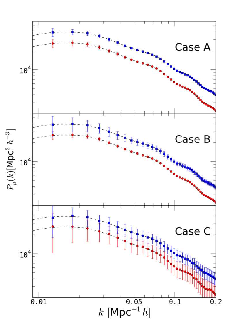
Figure 1: Estimated auto-spectra v. real auto-spectra. Filled (red) circles correspond to the power spectrum of the tracer 1, with $b_{1}={1.0}$, and filled (blue) squares correspond to the estimated power spectrum of the tracer 2, with bias $b_{2}=1.2$. The symbols and error bars correspond to the mean and to the variance, respectively, of 1000 realizations. The dased lines are the input (theoretical) spectra of the tracers, given their biases and our fiducial cosmology. The upper, middle and lower panels correspond to cases A, B and C, respectively (see Table 1). The error bars are the theoretical ones — i.e., the inverse of the Fisher matrix, Eq. (25).

With an initial guess for the biases and for the amplitude of the power spectrum, we can construct ${\cal{P}}_{\mu}$ and ${\cal{P}}=\sum_{\mu}{\cal{P}}_{\mu}$, plug them into the weights (33), and calculate the weighted density constrasts of Eq. (3.3). We then perform an FFt over $f(\vec{x})$ and $f_{\mu}(\vec{x})$, in order to obtain the integrand of Eq. (36). Taking proper care of the volume factors (in real and in Fourier space), this step should be analogous to the average over modes in Eq. (2.4.5) of FKP.

The next step is to subtract the biases of the estimators — the $\delta Q_{\mu,i}$ in Eq. (36) or, equivalently, Eq. (67). Assuming that averages over bins are such that $\langle A\,B\rangle_{i}\approx\langle A\rangle_{i}\,\langle B\rangle_{i}$, and taking a single value for all the $\alpha_{\mu}\to\alpha$, Eq. (40) can be rearranged to yield:

$$\delta Q_{\mu,i}=\frac{1+\alpha}{2}\int_{V_{i}}\frac{d^{3}x\,d^{3}k}{(2\pi)^{3}}\frac{\bar{n}_{\mu}}{(1+{\cal{P}})^{2}}\;.$$ (74)

With our choice of $\alpha=10^{-6}$, we find that $A_{\mu}\to\alpha$ to an excellent approximation, which means that the biases of the estimators are given only by Eq. (74) — see Sec. 3.3. Finally, the estimated power spectra are computed with the help of Eq. (3).

We present our results for the estimated spectra of two types of tracers in three cases, A, B and C — see Table 1 and Fig. 1. Case A represents a low-redshift survey which is highly complete, so both tracers are dense. Case B represents a low- or intermediate-redshift survey, with one dense species of tracer (type 1 — say, red galaxies) and one sparse species of tracer (type 2 — say, quasars). Case C represents a high-redshift survey, with two sparse types of tracers.

Our estimates were evaluated in evenly separated bandpowers with $\Delta k=0.005\,h$ Mpc^-1. We show the estimated spectra in Fig. 1, only up to $k=0.2\,h$ Mpc^-1 — slightly into the nonlinear regime but still below the Nyquist frequency, such that our results are not affected by discretization effects. When estimating the spectra we adopted a commonly used simplification, which is to fix the value of the matter power spectrum that is used in the weights, Eq. (33) — in our case, we found that fixing $P_{m}\to 10^{4}\,h^{-3}$ Mpc³ in the weights was a suitable choice. Our results did not change significantly over the dynamical range of interest when that value was multiplied by 2 or by 1/2.

5.3 Empirical v. theoretical covariances

We now check whether the theoretical covariance matrix (the inverse of the multi-tracer Fisher matrix) is a good approximation to the true (i.e., empirical) covariance matrix. If the theory is accurate, then the method is validated; if it is not, then the multi-tracer estimators are sub-optimal.

The empirical result was obtained from 1000 realizations. This was compared with the theoretical covariance — i.e., the inverse of the binned Fisher matrix of Eq. (25):

$$Cov(P_{\mu,i},P_{\nu,j})=\delta_{ij}\left[\frac{1}{P_{\mu,i}\,P_{\nu,i}}\int_{V_{i}}\frac{d^{3}x\,d^{3}k}{(2\pi)^{3}}{\cal{F}}_{\mu\nu}\right]^{-1}\;,$$ (75)

where ${\cal{F}}_{\mu\nu}$ was defined in Eq. (26).

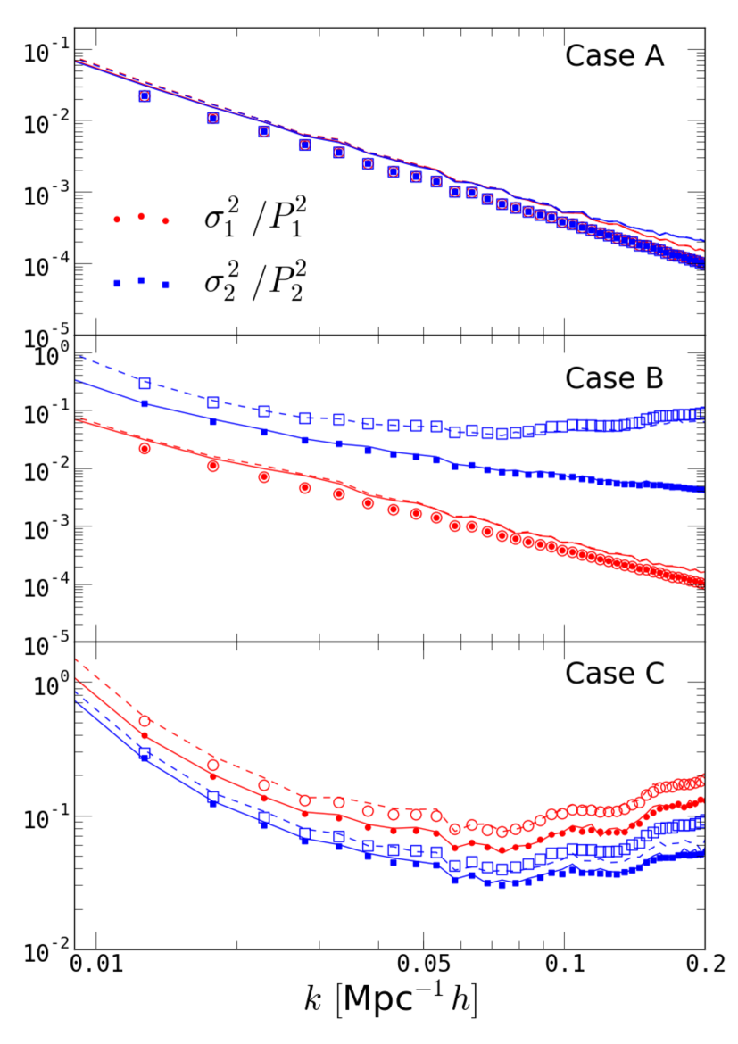
Figure 2: Theoretical v. empirical relative covariances of the auto-spectra, $Cov(P_{\mu,i},P_{\nu,i})/P_{\mu,i}P_{\nu,i}$. The upper, middle and lower panels correspond to cases A, B and C, respectively (see Table 1). Red circles and blue squares correspond to the theoretical covariances of the tracers 1 and 2, respectively. The lines of the same colors are the standard deviation of our 1000 lognormal mocks. Solid symbols and lines correspond to multi-tracer estimates, while open symbols and dashed lines correspond to FKP estimates. In case A (upper panel), since the two tracers have high signal-to-noise (both ${\cal{P}}_{1}\gg 1$ and ${\cal{P}}_{2}\gg 1$ in this range of scales), both the multi-tracer and the FKP formulas for the auto-covariances reduce to $Cov(P_{\mu,i},P_{\nu,i})/P_{\mu,i}P_{\nu,i}\simeq 2/V_{x,i}V_{k,i}\sim k^{-2}$ [see Eqs. (41)-(42)]. Hence, in this case most symbols and lines overlap. In most cases, the empirical covariances are slightly higher than the theoretical ones — as expected. In case B (middle panel), the covariance of spectrum of the sparse tracer species is significantly higher in the FKP method: in this case, the multi-tracer method reduces the uncertainty in the spectrum by a large factor.

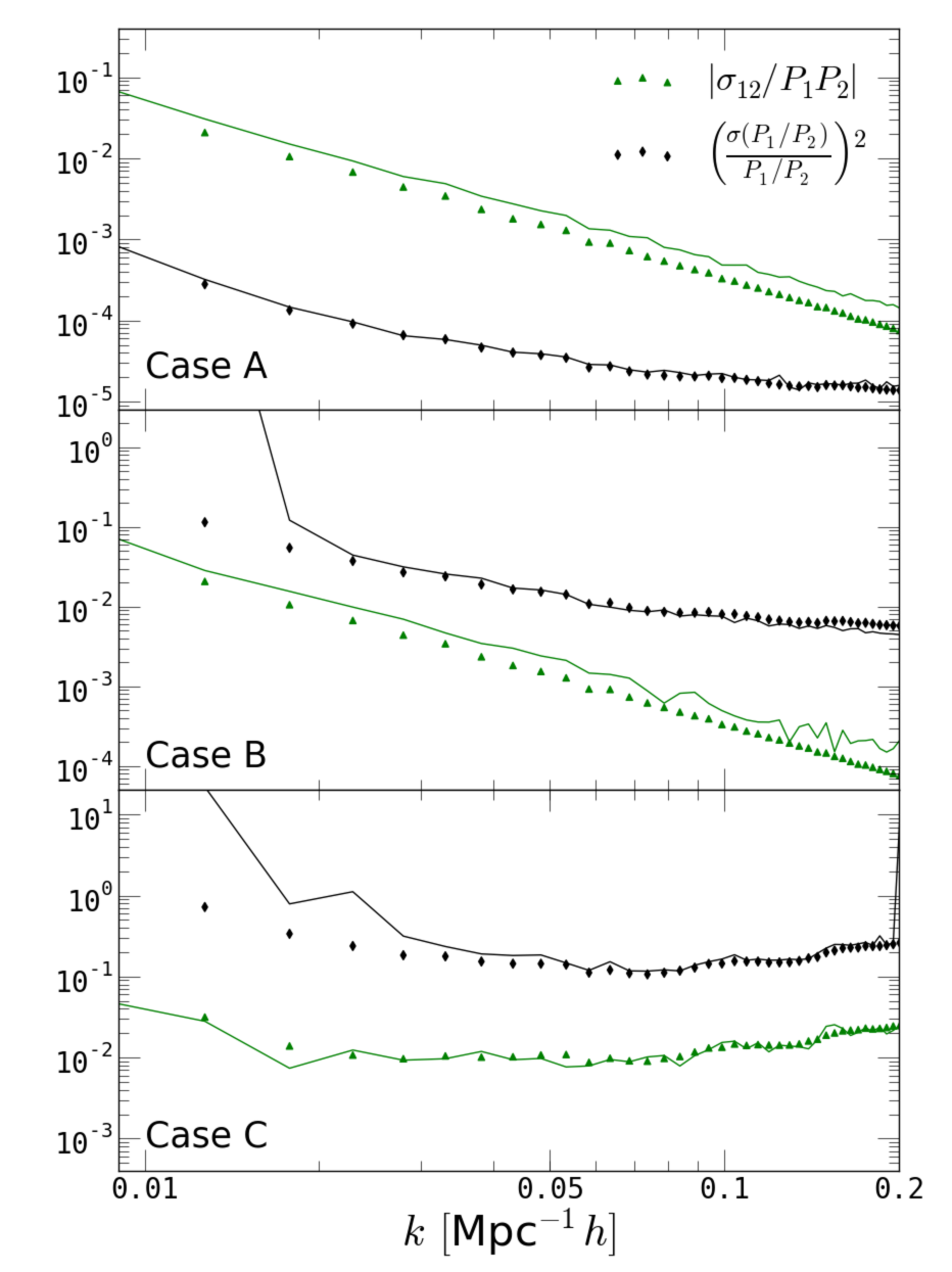
Figure 3: Theoretical v. empirical covariances of the cross-spectra and of the ratios between the spectra. The ratios were defined as $P_{1}/P_{2}$ (the relative covariance is identical for $P_{2}/P_{1}$). The upper, middle and lower panels correspond to cases A, B and C, respectively (see Table 1). Diamonds (black) correspond to the theoretical relative covariances of the cross-spectra, while triangles (green) correspond to the theoretical covariance for the ratios between the spectra (see text). The solid lines correspond to the empirical covariances, using the multi-tracer estimators (we do not show the results using the FKP estimator in these plots because it performs significantly worse compared with the multi-tracer estimators, and in any case the FKP method does not predict these covariances). Notice that in case C (lower panel) the covariance of the cross-correlations is negative, since ${\cal{P}}<1$ — see Eqs.(41)-(42). Notice also that in case A the ratio between the spectra has a much lower uncertainty than the cross-correlation (for an explanation, see the text).

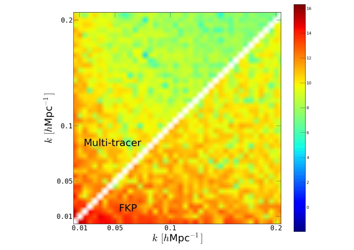
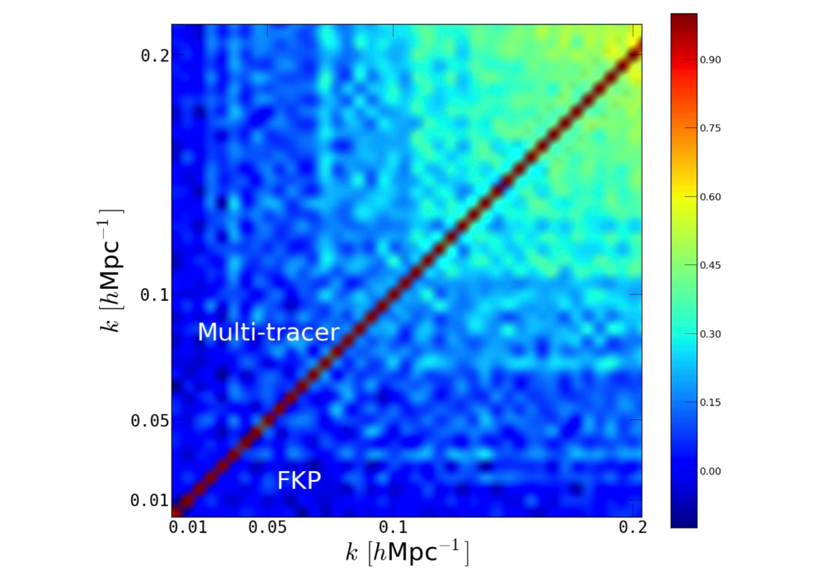
Figure 4: Upper panel: covariance matrix for tracer 2 in case B. The upper triangle is the result using the multi-tracer estimator, and the lower triangle results from using the FKP estimator. The multi-tracer technique performs significantly better on all scales. Lower panel: correlation matrix for tracer 2 in case A. Both the multi-tracer and the FKP estimators perform similarly regarding the correlations between Fourier bins. We checked that the estimators result in similar correlation matrices for both tracers, in the three different cases we analyzed.

In Fig. 2 we present the comparison between the theoretical and empirical covariances for the auto-spectra of the two species, obtained respectively from Eq. (75) and from taking the standard deviation of 1000 lognormal realizations. We find that our theoretical expression properly reproduces the behavior of the statistical fluctuations in all cases, matching more closely the variances when compared with the FKP method. The theoretical variances sometime underestimate slightly the empirical variance, which is consistent with the notion that the inverse of the Fisher matrix is an underestimate of the true covariance. This is in line with what is usually found in implementations of the FKP method. In cases B and C the multi-tracer estimator performs significantly better than the FKP estimator on all scales.

In Fig. 3 we compare the theoretical and empirical variances for the cross-spectra of the two tracers (green triangles), and for the ratios of the two spectra, $P_{1}/P_{2}$ (black diamonds). Since the FKP method cannot predict theoretical covariances in these two cases, we only show the multi-tracer theoretical variances. The theoretical variance for the ratio $P_{1}/P_{2}$ follows from the multi-tracer Fisher information matrix, Eq. (26), which can be diagonalized by a change of variables (Abramo & Leonard, 2013), where the new parameters (the “eigenvectors” of the Fisher matrix) are not the individual clustering strengths ${\cal{P}}_{\mu}$, but the total clustering strength, ${\cal{P}}$, and certain ratios between the clustering strengths. In particular, a diagonal Fisher matrix means that the degrees of freedom are independent — there are no cross-covariances. For two types of tracers, the variables which diagonalize the $2\times 2$ Fisher matrix are ${\cal{P}}={\cal{P}}_{1}+{\cal{P}}_{2}$, and ${\cal{P}}_{1}/{\cal{P}}_{2}$ (or, equivalently, ${\cal{P}}$ and ${\cal{P}}_{2}/{\cal{P}}_{1}$). As shown in Abramo & Leonard (2013), the Fisher matrix per unit of phase space volume for $\log(P_{1}/P_{2})$ is $F_{\rm ratio}={\cal{P}}_{1}\,{\cal{P}}_{2}/4(1+{\cal{P}}_{1}+{\cal{P}}_{2})$, from which follows that the relative covariance of that ratio is $[\int d^{3}x\,d^{3}k/(2\pi)^{3}F_{\rm ratio}]^{-1}$. This figure demonstrates the power of the multi-tracer technique to measure $P_{1}/P_{2}=B_{1}^{2}(z,k,\mu_{k})/B_{2}^{2}(z,k,\mu_{k})$, something that can be used to place stronger constraints not only the biases of the two species, but also on RSDs, NGs, etc.

The upper panel of Fig. 4 shows the covariance matrix for tracer 2 ($b_{2}=1.2$) in case B — i.e., $Cov_{22}^{(B)}(k_{i},k_{j})$. We exploited the symmetry of the covariance matrix under $k_{i}\leftrightarrow k_{j}$ in order to compare the multi-tracer and FKP estimators directly. In the lower panel of this figure we show the correlation matrix, defined as Corr${}_{ij}=Cov_{ij}/\sqrt{Cov_{ii}\,Cov_{jj}}$. We find that both the multi-tracer and the FKP estimators yield roughly similar correlation matrices, with weakly correlated bins up to scales $k\lesssim 0.1\,h$ Mpc^-1.

The upper panel of Fig. 4, together with the middle panels of Figs. 2 and 3, shows that in case B the multi-tracer estimator performs significantly better than the FKP estimator at all scales, with uncertainties up to one order of magnitude smaller for the spectrum of the sparse tracer. The multi-tracer technique is also clearly superior in estimating the auto-spectra in case C, when both tracers are sparse — see the lower panel of Fig. 2.

6 Including the 1-halo term

The fundamental object in this paper, which was used to derive the Fisher information matrix, as well as the optimal weights, is the pixel covariance. In the limit where bias and RSDs depend weakly on $\vec{k}$, the covariance can be approximated by Eq. (20). However, this is not a complete description: in addition to the “signal”, $P_{\alpha}=B_{\alpha}^{2}P_{m}$, and the shot noise, $\delta_{\alpha\beta}/\bar{n}_{\alpha}$, there is another source of correlations between the density contrasts of different species of tracers at different points in space: the 1-halo term of the power spectrum. According to the Halo Model (Cooray & Sheth, 2002), dark matter halos are the genuine tracers of the underlying matter density, while galaxies only trace the halos. In particular, this means that many galaxies may be hosted by the same halo, in which case they would be tracing the same features of the underlying fluctuations of the matter density.

This additional covariance between galaxy counts is expressed by the 1-halo term:

$$P^{1h}_{\alpha\beta}(k)=\frac{1}{\bar{n}_{\alpha}\,\bar{n}_{\beta}}\int d\ln M\,\frac{d\,\bar{n}_{h}}{d\ln M}\,u^{2}(k|M)\,\langle N_{\alpha}N_{\beta}\rangle_{M}\,\;,$$ (76)

where $d\,\bar{n}_{h}/d\ln M$ is the mass function for halos of mass $M$, $N_{\alpha}$ is the number of galaxies of type $\alpha$, and $u(k|M)$ is the Fourier transform of the halo profile (Cooray & Sheth, 2002). The expectation value is over the probability distribution function for the numbers of galaxies (the HOD) at a given halo mass. For the species of tracers which are typically used in cosmological surveys the 1-halo term is only relevant on small scales ($k\gtrsim 1\,h$/Mpc) — although, since $u(k\to 0)=1$, it still contributes a constant factor on large scales.

Inclusion of the 1-halo term would lead the approximated pixel covariance of Eq. (20) to assume the expression:

$$C_{\alpha\beta}(\vec{x},\vec{x}{\,}^{\prime})\rightarrow\delta_{D}(\vec{x},\vec{x}{\,}^{\prime})\times\left[\frac{\delta_{\alpha\beta}}{\bar{n}_{\alpha}}+P^{2h}_{\alpha\beta}+P^{1h}_{\alpha\beta}\right]\;,$$ (77)

where we write the 2-halo term $P^{2h}_{\alpha\beta}=B_{\alpha}B_{\beta}P_{m}$. In principle, if we are only interested on the properties of the clustering on large scales, this term can be included systematically, in every step of the calculations — see also Hamaus et al. (2010), in a similar context. These are straightforward computations, but for a general form of $P^{1h}_{\alpha\beta}$ there is no closed-form expression for the inverse of the pixel covariance matrix, which means that we cannot give explicit formulas for the Fisher matrix, the weights, the window functions, etc.

6.1 Fisher matrix of the 2-halo term for separable 1-halo terms

In some cases the populations of tracers are such that the 1-halo term is approximately separable, i.e., it can be expressed as a direct product of two terms, $P^{1h}_{\alpha\beta}\sim H_{\alpha}H_{\beta}$ — just as happens with the 2-halo term. We have checked that, for a class of HODs that is commonly used to describe red and blue galaxies (Zheng et al., 2005), all entries of the correlation matrix $P^{1h}_{\alpha\beta}/\sqrt{P^{1h}_{\alpha\alpha}P^{1h}_{\beta\beta}}$ are very close to unity, which justifies this approximation. However, we only verified this feature of the 1-halo term while ignoring the distinction between central and satellite galaxies, since it is not clear how to generalize $\langle N_{\alpha}N_{\beta}\rangle$ in that case. It would be interesting to find out whether this property holds for more realistic HODs.

If the 1-halo term is separable, it turns out that we can invert the covariance matrix. This result follows from the exquisite properties of matrices that can be written as $M_{\alpha\beta}=\delta_{\alpha\beta}+v_{\alpha}v_{\beta}+u_{\alpha}u_{\beta}$. This type of matrix appeared already in Section 2, where we showed that the inverse of $M_{v,\alpha\beta}=\delta_{\alpha\beta}+v_{\alpha}v_{\beta}$ is given by $M_{v,\alpha\beta}^{-1}=\delta_{\alpha\beta}-v_{\alpha}v_{\beta}/(1+v^{2})$, where $v^{2}=\sum_{\mu}v_{\mu}^{2}$.

As shown in Appendix B, the inverse of the matrix $M_{\alpha\beta}=\delta_{\alpha\beta}+v_{\alpha}v_{\beta}+u_{\alpha}u_{\beta}$ is:

$$M^{-1}_{\alpha\beta}=\sum_{\mu\nu}M_{v,\alpha\mu}^{-1/2}\,M_{u^{\prime},\mu\nu}^{-1}\,M_{v,\nu\beta}^{-1/2}\;,$$ (78)

where $M_{v,\alpha\beta}^{-1/2}=\delta_{\alpha\beta}-v_{\alpha}v_{\beta}/(1+v^{2}+\sqrt{1+v^{2}})$, and $u^{\prime}_{\alpha}=\sum_{\mu}M_{v,\alpha\mu}^{-1/2}u_{\mu}$.

After some algebra, using Eq. (78) we can express the inverse of the covariance, Eq. (77), as:

$$C_{\alpha\beta}^{-1}(\vec{x},\vec{x}{\,}^{\prime}) \rightarrow \delta_{D}(\vec{x},\vec{x}{\,}^{\prime})$$

$$\times\left[\delta_{\alpha\beta}\bar{n}_{\alpha}-\bar{n}_{\alpha}\frac{P^{2h}_{\alpha\beta}+P^{1h}_{\alpha\beta}+Y_{\alpha\beta}}{1+{\cal{T}}}\bar{n}_{\beta}\right]\;,$$

where the cross-term is:

$$Y_{\alpha\beta} = \sum_{\mu}\bar{n}_{\mu}\left(P^{2h}_{\alpha\mu}\,P^{1h}_{\mu\beta}+P^{1h}_{\alpha\mu}\,P^{2h}_{\mu\beta}\right.$$

$$\left.-P^{2h}_{\alpha\beta}\,P^{1h}_{\mu\mu}-P^{1h}_{\alpha\beta}\,P^{2h}_{\mu\mu}\right)\;,$$

and the term appearing of the denominator in Eq. (6.1) is:

$${\cal{T}}=\sum_{\mu}\bar{n}_{\mu}\,(P^{2h}_{\mu\mu}+P^{1h}_{\mu\mu})+\sum_{\mu\nu}\bar{n}_{\mu}\bar{n}_{\nu}(P^{2h}_{\mu\mu}\,P^{1h}_{\nu\nu}-P^{2h}_{\mu\nu}\,P^{1h}_{\mu\nu})\;.$$ (81)

Compare this result with Eq. (22). We detect some familiar expressions, in particular:

$${\cal{P}}=\sum_{\mu}\bar{n}_{\mu}B_{\mu}^{2}P_{m}\equiv\sum_{\mu}{\cal{P}}_{\mu}=\sum_{\mu}\bar{n}_{\mu}P^{2h}_{\mu\mu}\;.$$ (82)

It is now useful to rename the clustering strength of the 2-halo term as ${\cal{P}}_{\mu}\to{\cal{P}}^{2h}_{\mu}$, ${\cal{P}}\to{\cal{P}}^{2h}$, and to define the 1-halo clustering strength as ${\cal{P}}^{1h}=\sum_{\mu}\bar{n}_{\mu}P^{1h}_{\mu\mu}=\sum_{\mu}{\cal{P}}^{1h}_{\mu}$. The cross-terms mixing the 1-halo and the 2-halo terms appear in the combinations:

$$P^{c}_{\alpha\beta} \equiv \sum_{\mu}P^{2h}_{\alpha\mu}\,\bar{n}_{\mu}\,P^{1h}_{\mu\beta}\;,$$ (83)

$${\cal{P}}^{c}_{\alpha\beta} \equiv \bar{n}_{\alpha}\bar{n}_{\beta}P^{2h}_{\alpha\beta}P^{1h}_{\alpha\beta}\;.$$

Once again, we find it useful to define the dimensionless clustering strengths of these cross-terms, as was done for the 2-halo and the 1-halo terms. They are:

$${\cal{P}}^{c}_{\alpha} \equiv \bar{n}_{\alpha}P^{c}_{\alpha\alpha}=\sum_{\beta}{\cal{P}}^{c}_{\alpha\beta}\;,$$ (84)

$${\cal{P}}^{c} \equiv \sum_{\alpha}\bar{n}_{\alpha}P^{c}_{\alpha\alpha}=\sum_{\alpha\beta}{\cal{P}}^{c}_{\alpha\beta}\;.$$

With these definitions we find that:

$${\cal{T}}={\cal{P}}^{2h}+{\cal{P}}^{1h}+{\cal{P}}^{2h}{\cal{P}}^{1h}-{\cal{P}}^{c}\;.$$ (85)

Similarly, we get:

$$Y_{\alpha\beta}=P^{c}_{\alpha\beta}+P^{c}_{\beta\alpha}-P^{2h}_{\alpha\beta}\,{\cal{P}}^{1h}-P^{1h}_{\alpha\beta}\,{\cal{P}}^{2h}\;.$$ (86)

The Fisher matrix was defined in a generic sense in Eq. (18). That definition, as well as the construction of the optimal quadratic estimators, are valid for any Gaussian variables (Tegmark et al., 1998). In a related result, Smith & Marian (2015) recently derived an optimal estimator for the matter power spectrum, as well as the Fisher matrix for the power spectrum, including not only the 1-halo term, but also the 2- and 3-halo contributions to the trispectrum — most of which are, strictly speaking, non-Gaussian contributions. We did include the 1-halo term in the pixel covariance, as well as in the trispectrum, but only through the assumption of Gaussianity of the 4-point function. Due to the non-Gaussian terms that will appear in the trispectrum, our estimators are not exactly optimal. Nevertheless, in some sense our result are more general than those of Smith & Marian (2015), since the multi-tracer estimators can be employed not only in the computation of the matter power spectrum, but also for the biases and the RSDs.

Since we keep the assumption of Gaussianity, all we have to do is work out the algebra with the covariance of Eq. (77), and its inverse, given by Eq. (6.1). After a lengthy calculation, we find that the Fisher matrix which generalizes the expression in the integrand of Eq. (25) can be expressed as:

$${\cal{F}}_{\mu\nu}^{2h} = \frac{1}{4(1+{\cal{T}})^{2}}\left\{\;\left[(1+{\cal{P}}^{1h}){\cal{P}}^{2h}-{\cal{P}}^{c}\right]\right.$$ (87)

$$\times\left[\delta_{\mu\nu}{\cal{P}}^{2h}_{\mu}(1+{\cal{T}})-(1+{\cal{P}}^{1h}){\cal{P}}^{2h}_{\mu}{\cal{P}}^{2h}_{\nu}\right.$$

$$\left.+\;(1+{\cal{P}}^{2h}){\cal{P}}^{c}_{\mu\nu}+{\cal{P}}^{2h}_{\mu}{\cal{P}}^{c}_{\nu}+{\cal{P}}^{2h}_{\nu}{\cal{P}}^{c}_{\mu}\right]$$

$$\,+\;(1+{\cal{P}}^{1h})^{2}\,{\cal{P}}^{2h}_{\mu}{\cal{P}}^{2h}_{\nu}-({\cal{P}}^{c})^{2}{\cal{P}}^{c}_{\mu\nu}$$

$$\,-\left.(1+{\cal{P}}^{1h})\,({\cal{P}}^{2h}_{\mu}{\cal{P}}^{c}_{\nu}+{\cal{P}}^{2h}_{\nu}{\cal{P}}^{c}_{\mu})\;\right\}\;.$$

It can be easily verified that taking $P^{1h}_{\mu\nu}\to 0$ implies ${\cal{P}}^{c}_{\mu\nu}\to 0$, ${\cal{T}}\to{\cal{P}}^{2h}$, etc., and this expression reduces to the matrix ${\cal{F}}_{\mu\nu}$ which is inside the integral in Eq. (25). The matrix is also manifestly symmetric.

It can also be shown that this Fisher matrix is positive-definite, with positive diagonal terms and a positive determinant. This guarantees that the covariance of the 2-halo power spectrum is also positive-definite.

We should stress once again that the expression above is only valid in the approximation that the 1-halo term is separable, i.e., $P^{1h}_{\alpha\beta}/\sqrt{P^{1h}_{\alpha\alpha}P^{1h}_{\beta\beta}}\simeq\delta_{\alpha\beta}$. For a general form of the 1-halo term, the pixel covariance matrix cannot be inverted analytically, which means that there are no closed-form expressions for the Fisher matrix or for the optimal weights. One could still go ahead and compute them numerically, without any difficulty.

6.2 Fisher matrix and optimal weights for the 1-halo term

Now, suppose that what we are in fact interested in measuring the 1-halo term. The 1-halo term is now the “signal”, while the the 2-halo term, as well as shot noise, become the “noise”. This should in fact be the case for very small scales ($k\gg 1\,h$/Mpc), where the 1-halo term dominates over the 2-halo term (Cooray & Sheth, 2002).

The pixel covariance is still the same, as in Eq. (77), and, as long as the 1-halo term is separable, the inverse covariance is also unaltered — see Eq. (6.1). The basic difference is that now instead of writing $P^{2h}_{\alpha\beta}=B_{\alpha}(z,k,\mu_{k})B_{\beta}(z,k,\mu_{k})P_{m}(k)$, we assume that the 1-halo term can be written effectively as something like $P^{1h}_{\alpha\beta}=H_{\alpha}(z,k,\mu_{k})H_{\beta}(z,k,\mu_{k})U(k)$, where $U(k)$ contains information about the shape of the mean halo profile. This is a strong assumption: it means that, for $N$ species of tracers, the 1-halo term would have only $N$ degrees of freedom (the $P^{1h}_{\alpha}=H_{\alpha}^{2}U$), while the full expression in fact has $N(N-1)/2$ degrees of freedom.

Keeping the hypothesis that the 1-halo term is separable, all we need to do now, in order to find its Fisher matrix, is to exchange all the 2-halo terms by the 1-halo terms in Eq. (87). This procedure can also be used to define the optimal weights that ought to be used when extracting information about the 1-halo term from galaxy surveys.

Since many of the objects defined above are already symmetric under the exchange $P^{2h}_{\mu\nu}\leftrightarrow P^{1h}_{\mu\nu}$ (this includes ${\cal{T}}$, $Y_{\mu\nu}$ and ${\cal{P}}^{c}_{\mu\nu}$), the 1-halo Fisher matrix can be immediately written as:

$${\cal{F}}_{\mu\nu}^{1h} = \frac{1}{4(1+{\cal{T}})^{2}}\left\{\;\left[(1+{\cal{P}}^{2h}){\cal{P}}^{1h}-{\cal{P}}^{c}\right]\right.$$ (88)

$$\times\left[\delta_{\mu\nu}{\cal{P}}^{1h}_{\mu}(1+{\cal{T}})-(1+{\cal{P}}^{2h}){\cal{P}}^{1h}_{\mu}{\cal{P}}^{1h}_{\nu}\right.$$

$$\left.+\;(1+{\cal{P}}^{1h}){\cal{P}}^{c}_{\mu\nu}+{\cal{P}}^{1h}_{\mu}{\cal{P}}^{c}_{\nu}+{\cal{P}}^{1h}_{\nu}{\cal{P}}^{c}_{\mu}\right]$$

$$\,+\;(1+{\cal{P}}^{2h})^{2}\,{\cal{P}}^{1h}_{\mu}{\cal{P}}^{1h}_{\nu}-({\cal{P}}^{c})^{2}{\cal{P}}^{c}_{\mu\nu}$$

$$\,-\left.(1+{\cal{P}}^{2h})\,({\cal{P}}^{1h}_{\mu}{\cal{P}}^{c}_{\nu}+{\cal{P}}^{1h}_{\nu}{\cal{P}}^{c}_{\mu})\;\right\}\;.$$

For very small scales the 2-halo term can be neglected, and we are left just with the 1-halo terms.

The Fisher matrix in bins of $k$ is just as in Eq. (25):

$$F_{\mu,i\,;\,\nu,j}^{1h}=\frac{\delta_{ij}}{(P^{1h}_{\mu\nu})^{2}}\int_{V_{i}}\frac{d^{3}x\,d^{3}k}{(2\pi)^{3}}{\cal{F}}_{\mu\nu}^{1h}\;.$$ (89)

The optimal weights follow in a straightforward manner from this expression, just as was done for the 2-halo term.

6.3 Joint Fisher matrix for the 2-halo and 1-halo terms

The next obvious question is: what if we wish to estimate both the 2-halo and the 1-halo terms in a multi-tracer cosmological survey, simultaneously? The two contributions are clearly correlated, so their information contents are not independent. Evidently, on either very large or very small scales the correlations between the two are small, and one can treat the signal ($P^{2h}$ on large scales; $P^{1h}$ on small scales) as effectively independent of the noise. However, on intermediate scales (around $k\sim 1\,h$/Mpc) the 1-halo and the 2-halo terms may have significant correlations. Furthermore, the approximation of separable 1-halo term becomes more accurate on those intermediate scales.

The pixel covariance is still given by Eq. (77), and its inverse also remains unchanged, but we would now be considering our “signal” as the sum $P^{t}_{\mu}\equiv P^{2h}_{\mu}+P^{1h}_{\mu}$. The main difference is that the derivatives of the pixel covariance, which in the case when we neglected the 1-halo term were given by Eq. (24), should now be computed with respect to this total contribution, i.e.:

$$\frac{\partial C_{\alpha\beta}(\vec{x},\vec{x}{\,}^{\prime})}{\partial P^{t}_{\mu,i}} = \frac{\partial P^{2h}_{\mu,i}}{\partial P^{t}_{\mu,i}}\frac{\partial C_{\alpha\beta}(\vec{x},\vec{x}{\,}^{\prime})}{\partial P^{2h}_{\mu,i}}+\frac{\partial P^{1h}_{\mu,i}}{\partial P^{t}_{\mu,i}}\frac{\partial C_{\alpha\beta}(\vec{x},\vec{x}{\,}^{\prime})}{\partial P^{1h}_{\mu,i}}$$ (90)

$$= \int\frac{d^{3}k}{(2\pi)^{3}}e^{i\vec{k}\cdot(\vec{x}-\vec{x}{\,}^{\prime})}\left(\delta_{\alpha\mu}\delta^{i}_{\vec{x},\vec{k}}+\delta_{\beta\mu}\delta^{i}_{\vec{x}{\,}^{\prime},\vec{k}}\right)$$

$$\times\left[\frac{B_{\alpha}(\vec{x},\vec{k})B_{\beta}(\vec{x}{\,}^{\prime},\vec{k})}{2\,B_{\mu}^{2}(\vec{x}_{i},\vec{k}_{i})}\right.$$

$$+\left.\frac{H_{\alpha}(\vec{x},\vec{k})H_{\beta}(\vec{x}{\,}^{\prime},\vec{k})}{2\,H_{\mu}^{2}(\vec{x}_{i},\vec{k}_{i})}\right]\;.$$

Substitution of this expression, together with the inverse of the pixel covariance, into Eq.(18), leads to the full Fisher matrix for the power spectrum. This can be written as:

$$F^{t}_{\mu,i;\nu,j} = \delta_{ij}\int_{V_{i}}\frac{d^{3}x\,d^{3}k}{(2\pi)^{3}}\left[\frac{{\cal{F}}^{2h}_{\mu\nu}}{(P^{2h}_{\mu\nu,i})^{2}}+\frac{{\cal{F}}^{1h}_{\mu\nu}}{(P^{1h}_{\mu\nu,i})^{2}}\right.$$

$$+\left.\left(\frac{1}{P^{2h}_{\mu\mu,i}P^{1h}_{\nu\nu,i}}+\frac{1}{P^{2h}_{\nu\nu,i}P^{1h}_{\mu\mu,i}}\right){\cal{F}}^{c}_{\mu\nu}\right]\;,$$

where ${\cal{F}}^{c}_{\alpha\beta}$ contains the cross-terms between the 1-halo and the 2-halo terms which follow from Eq. (90). Expressing the inverse covariance of Eq. (6.1) in terms of $C^{-1}_{\alpha\beta}(\vec{x},\vec{x}{\,}^{\prime})=\delta_{D}(\vec{x},\vec{x}{\,}^{\prime})D_{\alpha\beta}$, the information mixing between the 1-halo and 2-halo terms is given by:

$${\cal{F}}^{c}_{\mu\nu} = \frac{1}{8}\sum_{\alpha\beta}\left(P^{1h}_{\alpha\beta}D_{\alpha\beta}\,P^{2h}_{\mu\nu}D_{\mu\nu}+P^{2h}_{\alpha\beta}D_{\alpha\beta}\,P^{1h}_{\mu\nu}D_{\mu\nu}\right.$$ (92)

$$+\left.P^{2h}_{\nu\alpha}D_{\alpha\mu}P^{1h}_{\mu\beta}D_{\beta\nu}+P^{1h}_{\nu\alpha}D_{\alpha\mu}P^{2h}_{\mu\beta}D_{\beta\nu}\right)\;.$$

It is trivial to obtain the full expression, although it turns out to be rather long. It can be significantly simplified if we employ two additional auxiliary definitions:

$$Z^{1,2h}_{\mu\nu} \equiv \sum_{\alpha}P^{1,2h}_{\mu\alpha}D_{\alpha\nu}\;,$$ (93)

$$W^{1,2h}_{\mu\nu} \equiv P^{1,2h}_{\mu\nu}D_{\mu\nu}\;.$$ (94)

In terms of these variables we have, e.g.:

$$Z^{2h}_{\mu\nu}=\frac{\bar{n}_{\nu}}{1+{\cal{T}}}\left[\left(1+2{\cal{P}}^{2h}+{\cal{P}}^{1h}\right)P^{2h}_{\mu\nu}+P^{c}_{\mu\nu}\right]\;,$$ (95)

and

$$W^{2h}_{\mu\nu} = \delta_{\mu\nu}{\cal{P}}^{2h}_{\mu}+\frac{\left(1-{\cal{P}}^{1h}\right){\cal{P}}^{2h}_{\mu}{\cal{P}}^{2h}_{\nu}}{1+{\cal{T}}}$$

$$+\frac{{\cal{P}}^{2h}_{\mu}{\cal{P}}^{c}_{\nu}+{\cal{P}}^{2h}_{\nu}{\cal{P}}^{c}_{\mu}+\left(1-{\cal{P}}^{2h}\right){\cal{P}}^{c}_{\mu\nu}}{1+{\cal{T}}}\;,$$

as well as the analogous expressions obtained by exchanging $1h\leftrightarrow 2h$. In terms of these definitions we have:

$${\cal{F}}^{c}_{\mu\nu} = \frac{1}{8}\left[Z^{1h}W^{2h}_{\mu\nu}+Z^{2h}W^{1h}_{\mu\nu}\right.$$

$$+\left.\sum_{\alpha}\left(Z^{2h}_{\mu\alpha}Z^{1h}_{\alpha\nu}+Z^{1h}_{\mu\alpha}Z^{2h}_{\alpha\nu}\right)\right]\;,$$

where $Z=\sum_{\mu}Z_{\mu\mu}=\sum_{\mu\nu}W_{\mu\nu}$. In fact, these definitions are also helpful when computing ${\cal{F}}^{2h}_{\mu\nu}$ (taking all $Z\to Z^{2h}$ and $W\to W^{2h}$) and ${\cal{F}}^{1h}_{\mu\nu}$ (taking all $Z\to Z^{1h}$ and $W\to W^{1h}$).

7 Conclusions

We have obtained optimal estimators for the Fourier analysis of multi-tracer cosmological surveys. The formulas were derived in Sec. 3, and a practical algorithm for the Fourier analysis of multi-tracer surveys was summarized in Sec. 5.2. Those are the main results of this paper.

The multi-tracer technique estimates the individual redshift-space power spectra for each tracer, $P_{\alpha}(z,k,\mu_{k})$, taking into account the covariance between the tracers which is induced by the large-scale structure. In contrast to the estimators obtained by Percival et al. (2003) or Smith & Marian (2015), which are suited for estimating the underlying matter power spectrum after fixing the biases and the RSDs, our optimal estimators can be used to measure both the power spectrum, the biases, the shape of RSDs, etc. In particular, our estimators facilitate measurements of RSDs, scale-dependent bias and non-Gaussianities from cosmological surveys of multiple tracers, helping realize the potential for determining those physical parameters to an accuracy which is not limited by cosmic variance (Seljak, 2009; McDonald & Seljak, 2008; Gil-Marín et al., 2010; Hamaus et al., 2011; Abramo & Leonard, 2013).

We also included the contribution from the 1-halo term in our calculations (Sec. 6). Although on very large scales ($k\ll 1\,h$ Mpc^-1) the 2-halo term is dominant, the 1-halo term gives a nearly-constant contribution in that limit, adding to shot noise — and, unlike shot noise, it does affect the cross-correlations.

It is important to stress that our formulas are relatively simple generalizations of those by FKP (Feldman et al., 1994) and PVP (Percival et al., 2003), so readers familiar with these standard methods should have no trouble implementing the multi-tracer technique. We tested the estimators (see Sec. 5) in a wide variety of situations, and they performed quite robustly — in many instances, significantly better than the FKP method. It should now be straightforward to combine cosmological surveys targeting different types of galaxies, quasars and other tracers of large-scale structure.

Acknowledgements – We would like to thank FAPESP, CNPq, and the University of São Paulo’s NAP LabCosmos for financial support.

Appendix A Degenerate tracers in the basis of the auto-power spectra

Suppose we have $N$ types of tracers, but we would like to combine the last 2 of those tracers into a single species, for a new total of $N-1$ tracers. For simplicity, let’s regard our original parameters as ${\cal{P}}_{\mu}$ ($\mu=1\ldots N$). We would like to change variables to ${\cal{P}}^{\prime}_{a}$ ($a=1\ldots N-1$), where ${\cal{P}}^{\prime}_{a}={\cal{P}}_{a}$ for $a=1,\ldots N-2$, and the new tracer species is constructed by combining the last two tracers, ${\cal{P}}^{\prime}_{N-1}={\cal{P}}_{N-1}+{\cal{P}}_{N}$. When the biases of the two species which are combined into one are identical, $B_{N-1}=B_{N-2}=B^{\prime}_{N-1}$, this linear combination ensures that ${\cal{P}}^{\prime}_{N-1}=(\bar{n}_{N-1}+\bar{n}_{N})B^{\prime 2}_{N-1}P_{m}$, so clearly $\bar{n}^{\prime}_{N-1}=\bar{n}_{N-1}+\bar{n}_{N}$ — i.e., the total number of galaxies of the new species is the sum of the number of galaxies of the two original species.

The Jacobian for the transformation ${\cal{P}}^{\prime}_{a}\to{\cal{P}}_{\mu}$ is $\partial{\cal{P}}^{\prime}_{a}/\partial{\cal{P}}_{\mu}$, and this Jacobian equals $\delta_{a\mu}$ when $\mu<N-1$, it vanishes if $a=N-1$ and $\mu<N-1$, and it is equal to 1 if $a=N-1$ and $\mu\geq N-1$.

However, what we need for the new Fisher matrix is the Jacobian for the inverse transformation, ${\cal{P}}_{\mu}\to{\cal{P}}^{\prime}_{a}$, i.e., $J_{\mu a}=(\partial{\cal{P}}_{\mu}/\partial{\cal{P}}^{\prime}_{a})^{-1}$. But this turns out to be a very simple matrix: $J_{\mu a}=\delta_{\mu a}$ when $\mu<N-1$, it vanishes if $a=N-1$ and $\mu<N-1$, and when $a=N-1$ and $\mu\geq N-1$ the Jacobian is equal to ${\cal{P}}_{\mu}/{\cal{P}}^{\prime}_{N-1}={\cal{P}}_{\mu}/({\cal{P}}_{N-1}+{\cal{P}}_{N-1})$ — see also the discussion at the beginning of Sec. 4.

Hence, in the new variables the Fisher matrix (or, more precisely, the Fisher information density per unit of phase space volume) is:

$$F^{\prime}_{ab}=F[{\cal{P}}^{\prime}_{a},{\cal{P}}^{\prime}_{b}]=\sum_{\mu\nu}^{N}J_{\mu a}\,\frac{{\cal{F}}_{\mu\nu}}{{\cal{P}}_{\mu}\,{\cal{P}}_{\nu}}\,J_{\nu b}\;,$$ (97)

where ${\cal{F}}_{\mu\nu}=F[\log{\cal{P}}_{\mu},\log{\cal{P}}_{\nu}]$ — see Eq. (26). This turns out to be given by:

$$F^{\prime}_{ab}=\left(\begin{array}[]{c;{2pt/2pt}c}\frac{1}{{\cal{P}}^{\prime}_{a}\,{\cal{P}}^{\prime}_{b}}{\cal{F}}_{ab}&\frac{1}{{\cal{P}}'_{a} {\cal{P}}'_{N-1}} \sum_{\nu=N-1}^N {\cal{F}}_{a\nu}\\ &\\ \hdashline[2pt/2pt]\\ {\rm Sym}&\frac{1}{({\cal{P}}'_{N-1})^{2}} \sum_{\mu,\nu=N-1}^N {\cal{F}}_{\mu\nu}\end{array}\right)\;,$$ (98)

where the upper left block is an $(N-2)\times(N-2)$ matrix, the right block is an $1\times(N-2)$ column, the lower left block is an $(N-2)\times 1$ row, and the lower right block is a single entry. Hence, the resulting $(N-1)$-dimensional Fisher matrix is given simply by summing the lines and columns corresponding to the two tracers which were combined into a single type.

Now, it can be easily verified from Eq. (26) that summing any two lines and columns of the fisher matrix ${\cal{F}}_{\mu\nu}$ yields precisely the Fisher matrix where the new entries correspond to the Fisher information for the sum of the clustering strengths of the two species that were combined. In other words, if we take Eq. (26) and use ${\cal{P}}^{\prime}_{a}$ to compute ${\cal{F}}^{\prime}_{ab}=F[\log{\cal{P}}^{\prime}_{a},\log{\cal{P}}^{\prime}_{b}]$, then the Fisher matrix $F^{\prime}_{ab}={\cal{F}}^{\prime}_{ab}/{\cal{P}}^{\prime}_{a}{\cal{P}}^{\prime}_{b}$ is identical to Eq. (98).

This argument can be iterated to show that combining any number of tracers into a single species corresponds to adding their clustering strengths, and this operation results in a simple sum of the Fisher information of those tracers.

Appendix B Inversion of the covariance matrix

Consider a matrix of the form $M_{v}=\mathbb{1}\,+\,v\otimes v$ — i.e., $M_{v,\,\mu\nu}=\delta_{\mu\nu}\,+\,v_{\mu}v_{\nu}$. As discussed in Section 2, it can be shown that:

$$M^{-1}_{v}=\mathbb{1}-\frac{v\otimes v}{1+v^{2}}\;,$$ (99)

where $v^{2}={\rm Tr}(v\otimes v)=\sum_{\alpha}v_{\alpha}v_{\alpha}$. This is in fact a special case of the Sherman-Morrison-Woodbury formula (Woodbury, 1950).

The matrix $M_{v}$ also has a simple “square root”, as well as an “inverse square root”, given by:

$$M^{1/2}_{v} = \mathbb{1}+\frac{v\otimes v}{1+\sqrt{1+v^{2}}}\;$$ (100)

$$M^{-1/2}_{v} = \mathbb{1}-\frac{v\otimes v}{1+v^{2}+\sqrt{1+v^{2}}}\;,$$ (101)

where $M_{v}^{-1/2}\cdot M_{v}^{-1/2}=M_{v}^{-1}$ and $M_{v}^{-1/2}\cdot M_{v}=M_{v}^{1/2}$, from which follows that:

$$M_{v}^{-1/2}\cdot M_{v}\cdot M_{v}^{-1/2}=\mathbb{1}\;.$$ (102)

Now, take a matrix $M=M_{v}+u\otimes u$. The first piece of that matrix can be diagonalized following the procedure outlined above, so we have that:

$$M_{v}^{-1/2}\cdot M\cdot M_{v}^{-1/2} = \mathbb{1}+(M_{v}^{-1/2}\cdot u)\otimes(u\cdot M_{v}^{-1/2})$$ (103)

$$= \mathbb{1}+u^{\prime}\otimes u^{\prime}\;,$$

where $u^{\prime}=M_{v}^{-1/2}\cdot u$ (i.e., $u^{\prime}_{\alpha}=\sum_{\mu}M^{-1/2}_{v,\alpha\mu}u_{\mu}$). But the matrix of Eq. (103) can now be inverted using the equivalent of Eq. (99), and moreover it has an inverse square root $M_{u^{\prime}}^{-1/2}$, as in Eq. (101). Therefore, we have that:

$$M_{u^{\prime}}^{-1/2}\cdot M_{v}^{-1/2}\cdot M\cdot M_{v}^{-1/2}\cdot M_{u^{\prime}}^{-1/2}=\mathbb{1}\;.$$

Therefore, the inverse of the matrix $M$ is given by:

$$M^{-1} = M_{v}^{-1/2}\cdot M_{u^{\prime}}^{-1/2}\cdot M_{u^{\prime}}^{-1/2}\cdot M_{v}^{-1/2}$$ (104)

$$= M_{v}^{-1/2}\cdot M_{u^{\prime}}^{-1}\cdot M_{v}^{-1/2}\;.$$

Of course, one could equally write this inverse as:

$$M^{-1}=M_{u}^{-1/2}\cdot M_{v^{\prime}}^{-1}\cdot M_{u}^{-1/2}\;,$$

where $v^{\prime}=M_{u}^{-1/2}\cdot v$.

References

- Abbott et al. (2005) Abbott, T. et al., 2005, preprint (arXiv:astro-ph/0510346)
- Abell et al. (2009) Abell, P., et al., 2009, preprint (arXiv:0912.0201)
- Abramo (2012) Abramo, L. R., 2012, MNRAS, 420, 3
- Abramo et al. (2012) Abramo, L. R., et al., 2012, MNRAS, 423, 335
- Abramo & Leonard (2013) Abramo, L. R., Leonard, K. E., 2013, MNRAS, 432, 318
- Adelman-McCarthy et al. (2008a) Adelman-McCarthy, J. K., et al., 2008a, VizieR Online Data Catalog, 2282, 0
- Adelman-McCarthy et al. (2008b) Adelman-McCarthy, J. K., et al., 2008b, ApJS, 175, 297
- Alcock & Paczynski (1979) Alcock, C., Paczynski, B., 1979, Nature, 281, 358
- Anderson et al. (2012) Anderson, L., et al., 2012, MNRAS, 427, 3435
- Anderson et al. (2014) Anderson, L., et al., 2014, MNRAS, 439, 83
- Bandura et al. (2014) Bandura, K., et al., 2014, preprint (arXiv:1406.2288)
- Bardeen et al. (1986) Bardeen, J. M., Bond, J. R., Kaiser, N., Szalay, A. S., 1986, ApJ, 304, 15
- Bartolo et al. (2004) Bartolo, N., Komatsu, E., Matarrese, S., & Riotto, A., 2004, Phys. Rept., 402, 103
- Battye et al. (2012) Battye, R., et al., 2012, preprint (arXiv:1209.1041)
- Benson et al. (2000) Benson, A. J., Cole, S., Frenk, C. S, Baugh, C. M., Lacey, C. G., MNRAS, 311, 793-808
- Benítez et al. (2009) Benítez, N., et al., 2009, ApJ, 691, 241
- Benítez et al. (2014) Benítez, N., et al., 2014, preprint (arXiv:1403.5237)
- (18) BigBOSS: http://bigboss.lbl.gov/ .
- Blake & Glazebrook (2003) Blake, C., Glazebrook, K., 2003 ApJ, 594, 665
- Blake et al. (2011) Blake, C., et al., 2011, MNRAS, 415, 2876
- Blake et al. (2013) Blake, C., et al., 2013, MNRAS, 436, 3089
- Bonoli & Pen (2008) Bonoli, S., Pen, U.-L., 2008, MNRAS, 396, 1610
- (23) BOSS: http://cosmology.lbl.gov/boss/ .
- Bull et al. (2014) Bull, P., Ferreira, P., Patel, P., Santos, M. G., 2014, 1405.1452
- Cai & Bernstein (2011a) Cai, Y.-C., Bernstein, G. M., MNRAS, 416, 3009
- Cai & Bernstein (2011b) Cai, Y.-C., Bernstein, G. M., MNRAS, 422, 1045
- Cai et al. (2011) Cai, Y.-C., Bernstein, G. M., Sheth, R. K., 2011, MNRAS, 412, 995
- Cole et al. (2005) Cole, S., et al., 2005, MNRAS, 362, 505
- Coles & Jones (1991) Coles, P.,Jones, B., 1991, MNRAS, 248, 1
- Cooray & Sheth (2002) Cooray, A., Sheth, R., 2002, Phys. Rept., 372, 1
- Croom et al. (2005) Croom, S., et al., 2005, MNRAS, 356, 415
- da Ângela et al. (2005) da Ângela, J., et al., 2005, MNRAS, 360, 1040
- Dalal et al. (2008) Dalal, N., Doré, O., Huterer, D., Shirokov, A., 2008, Phys. Rev., D77, 123514
- Dekel & Lahav (1999) Dekel, A., Lahav, O., 1999, ApJ, 520, 24
- Eisenstein et al. (1999) Eisenstein, D. J., Hu, W., Tegmark, M., 1999, ApJ, 518, 2
- Ellis et al. (2012) Ellis, R., Takada, M., et al., The PFS Team, preprint (arXiv:1206.0737)
- Feldman et al. (1994) Feldman, H. A., Kaiser, N., Peacock, J. A., 1994, ApJ, 426, 23
- Ferramacho et al. (2014) Ferramacho, L. D., Santos, M. G., Jarvis, M. J., Camera, S., 2014, MNRAS, 442, 2511
- Gil-Marín et al. (2010) Gil-Marín, H., Wagner, C., Verde, L., Jimenez, R., Heavens, A., 2011, MNRAS, 407, 772
- Hamaus et al. (2010) Hamaus, N., Seljak, U., Desjacques, V., Smith, R., Baldauf, T, 2010, Phys. Rev., D82, 043515
- Hamaus et al. (2011) Hamaus, N., Seljak, U., Desjacques, V., 2011, Phys. Rev., D84, 083509
- Hamaus et al. (2012) Hamaus, N., Seljak, U., Desjacques, V., 2012, Phys. Rev., D86, 103513
- Hamaus et al. (2014) Hamaus, N., Sutter, P. M., Lavaux, G., Wandelt, B. D., 2014, MNRAS
- Hamilton (2005a) Hamilton, A. J. S., 2005a, Lect. Notes Phys., 665, 415, astro-ph/0503603.
- Hamilton (2005b) Hamilton, A. J. S., 2005b, Lect. Notes Phys., 665, 433, arXiv: astro-ph/0503604.
- Hill (2008) Hill, G. J., et al., 2008, in “Panoramic Views of the Universe”, ASP Conf. Series, 399, 115
- Kaiser (1987) Kaiser, N., 1987, MNRAS, 227, 1
- Leistedt et al. (2013) Leistedt, B., Peiris, H. V., Mortlock, D. J., Benoit-Lévy, A., Pontzen, A., 2013, MNRAS, 435, 1857
- Leistedt & Peiris (2014) Leistedt, B., Peiris, H. V., 2014, MNRAS, 444, 2
- Lewis, Challinor & Lasenby (2000) Lewis, A., Challinor, A., Lasenby, A., 2000, ApJ, 538, 473
- Linder (2005) Linder, E., 2005, Phys. Rev., D72, 043529
- Martinez & Saar (2001) Martinez, V., Saar, E., 2001, “Statistics of the Galaxy Distribution” (CRC Press, 2001)
- McDonald & Seljak (2008) McDonald, P., Seljak, U., 2009, JCAP, 0910, 007
- (54) PAN-STARRS: http://pan-starrs.ifa.hawaii.edu/public/
- Percival et al. (2003) Percival, W. J., Verde, L., Peacock, J. A., 2004, MNRAS, 347, 645
- Raccanelli et al. (2012) Raccanelli, A., et al., 2012, MNRAS, 436, 89
- Rau (2009) Rau, A., et al., 2009, Publ. Astron. Soc. Pac., 121, 1334
- Ross et al. (2009) Ross, A., et al., 2009, ApJ, 697, 1634
- Sawangwit et al. (2012) Sawangwit, A., et al., 2012, MNRAS, 420, 1916
- Scoville et al. (2007) Scoville, N., et al., 2007, ApJS, 172, 1
- Sefusatti & Komatsu (2007) Sefusatti, E., & Komatsu, E., 2007, Phys. Rev., D76, 083004
- Seljak (2009) Seljak, U., 2009, Phys. Rev. Lett., 102, 021302
- Seljak et al. (2009) Seljak, U., Hamaus, N., Desjacques, V., 2009, Phys. Rev. Lett., 103, 091303
- Seo & Eisenstein (2003) Seo, H.-J., Eisenstein, D. J., 2003, ApJ, 598, 720
- Shen et al. (2007) Shen, Y., et al., 2007, AJ, 133, 2222
- Slosar et al. (2008) Slosar, A., Hirata, C., Seljak, U., Ho, S., Pabmanabhan, N., 2008, JCAP, 09, 31
- Slosar (2009) Slosar, A., 2009, JCAP, 03, 004
- Slosar et al. (2013) Slosar, A., et al., 2013, JCAP, 04, 026
- Smith (2009) Smith, R. E., 2009, MNRAS, 400, 851
- Smith, Desjacques & Marian (2011) Smith, R. E., Desjacques, V., Marian, L., 2011, Phys. Rev., D83, 043526
- Smith & Marian (2014) Smith, R. E., Marian, L., 2014, preprint (arXiv:1406.1800)
- Smith & Marian (2015) Smith, R. E., Marian, L., 2015, preprint (arXiv:1503.06830)
- Smith, Scoccimarro & Sheth (2009) Smith, R. E., Scoccimarro, R., Sheth, R. K., 2007, Phys. Rev., D75, 063512
- (74) SUMIRE: http://sumire.ipmu.jp/en/
- Swanson et al. (2008) Swanson, M., Tegmark, M., Blanton, M., Zehavi, I., 2008, MNRAS, 385, 1635
- Tegmark et al. (1997) Tegmark, M., Taylor, A. N. , Heavens, A. F., 1997, ApJ, 480, 22
- Tegmark (1997) Tegmark, M., 1997, Phys. Rev. Lett., 79, 3806
- Tegmark et al. (1998) Tegmark, M., Hamilton, A. J. S., Strauss, M. A., Vogeley, M. S. , Szalay, A. S., 1998, ApJ, 499, 555
- Verde et al. (2000) Verde, L., Wang, L., Heavens, A. F., Kamionkowski, M., 2000, MNRAS, 313, 141
- Wang (2006) Wang, Y. 2006, ApJ, 647, 1
- Weinberg (2002) Berlind, A. A., Weinberg, D. H., 2002, ApJ, 575, 587
- White et al. (2008) White, M., Song, Y.-S., Percival, W. J., 2008, MNRAS, 397, 1348
- Woodbury (1950) Woodbury, M. A., 1950, Memorandum Rept. 42, Statistical Research Group, Princeton University, Princeton, NJ
- Yahata et al. (2005) Yahata, K., et al., 2005, PASJ, 57, 529
- York et al. (2000) York, D. G., et al., 2000, AJ, 120, 1579
- Zheng et al. (2005) Zheng, Z., et al., 2005, ApJ, 633, 791