Azimuthal Metallicity Structure in the Milky Way Disk

Abstract

Elemental abundance patterns in the Galactic disk constrain theories of the formation and evolution of the Milky Way. H ii region abundances are the result of billions of years of chemical evolution. We made radio recombination line and continuum measurements of 21 H ii regions located between Galactic azimuth $Az=90$$\,{}^{\circ}$$-130$$\,{}^{\circ}$, a previously unexplored region. We derive the plasma electron temperatures using the line-to-continuum ratios and use them as proxies for the nebular [O/H] abundances, because in thermal equilibrium the abundance of the coolants (O, N, and other heavy elements) in the ionized gas sets the electron temperature, with high abundances producing low temperatures. Combining these data with our previous work produces a sample of 90 H ii regions with high quality electron temperature determinations. We derive kinematic distances in a self-consistent way for the entire sample. The radial gradient in [O/H] is $-0.082\pm\ 0.014$$\rm\,dex\,kpc^{-1}$ for $Az=90$$\,{}^{\circ}$$-130$$\,{}^{\circ}$, about a factor of two higher than the average value between $Az=0$$\,{}^{\circ}$$-60$$\,{}^{\circ}$. Monte Carlo simulations show that the azimuthal structure we reported for $Az=0$$\,{}^{\circ}$$-60$$\,{}^{\circ}$ is not significant because kinematic distance uncertainties can be as high as 50% in this region. Nonetheless, the flatter radial gradients between $Az=0$$\,{}^{\circ}$$-60$$\,{}^{\circ}$ compared with $Az=90$$\,{}^{\circ}$$-130$$\,{}^{\circ}$, are significant within the uncertainty. We suggest that this may be due to radial mixing from the Galactic Bar whose major axis is aligned toward $Az\sim\ 30$$\,{}^{\circ}$.

1 Introduction

Measurements of the elemental abundance distribution in the Galactic disk provide important constraints to the formation and evolution of the Milky Way (e.g., Pagel, 1997). Searle (1971) was the first to detect radial gradients in nearby galaxies using collisionally excited lines (CELs) of oxygen, nitrogen, and sulfur from H ii regions. Observations of CELs in the Milky Way disk are more sensitive, but they are affected by dust and it is difficult to determine distances which are necessary to derive radial abundance gradients. Nevertheless, radial gradients have been detected in the Galactic disk and interpreted as higher processing of metals by stars in the central regions of the Milky Way (e.g., Henry & Worthey, 1999; Tosi, 2000).

The primary metallicity tracers in the Galactic disk are open clusters (e.g., Janes, 1979; Twarog et al., 1997; Friel et al., 2002; Young et al., 2012; Frinchaboy et al., 2013), Cepheids (e.g., Caputo et al., 2001; Lemasle et al., 2013; Korotin et al., 2014), OB stars (e.g., Fitzsimmons et al., 1990; Rolleston et al., 2000; Daflon & Cunha, 2004), red giant stars (e.g., Hayden et al., 2013; Boeche, et al., 2014; Bovy et al., 2014), planetary nebulae (e.g., Maciel et al., 2003; Pottasch & Bernard-Salas, 2006; Stanghellini & Haywood, 2010; Henry et al., 2010), and H ii regions (e.g., Peimbert, 1978; Shaver et al., 1983; Afflerbach et al., 1997; Deharveng et al., 2000; Rudolph et al., 2006; Esteban et al., 2013). Typically, Fe/H is used as a proxy for metallicity in stars using absorption lines, whereas O/H is the main metallicity diagnostic in the interstellar medium (ISM) using emission lines (Henry & Worthey, 1999). Other abundance ratios (e.g., $\alpha$/Fe) provide additional information (Hayden et al., 2013). Each tracer has advantages and disadvantages.

Here we explore the metallicity distribution of the Milky Way using H ii regions. They are created by the hydrogen ionizing photons from massive OB stars and can be detected at infrared (IR) and radio wavelengths throughout the Galactic disk. Since H ii regions are young ($<10$$\,{\rm Myr}$), their abundances provide a measure of the nuclear processing of many stellar generations. H ii regions with maser parallax measurements have accurate distances that are critical for exploring Galactic azimuthal metallicity structure. Optical and IR CELs are the primary diagnostics of metallicity in H ii regions, but more recently optical recombination lines (ORLs) have been used (e.g., Esteban et al., 2005). Radio recombination line (RRL) and thermal continuum emission provide an accurate measure of the nebular electron temperature which has been used to indirectly probe metallicity (Churchwell & Walmsley, 1975; Churchwell et al., 1978; Mezger et al., 1979; Lichten et al., 1979; Wilson et al., 1979; Wink et al., 1983; Afflerbach et al., 1996; Quireza et al., 2006; Balser et al., 2011). Such radio diagnostics of H ii regions yield an extinction free tracer to map the metallicity distribution across the entire Milky Way disk.

2 Observations and Data Reduction

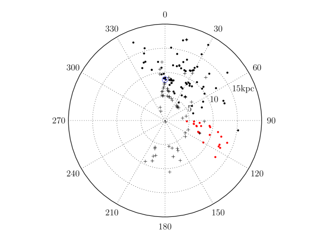
Here we expand on our previous efforts of using RRL and continuum emission from H ii regions throughout the Galactic Plane to derive electron temperatures that are used as a proxy for metallicity. Figure 1 shows the Galactic distribution of H ii regions with derived electron temperatures using data from the National Radio Astronomy Observatory (NRAO) 140 Foot telescope (Quireza et al., 2006, black crosses; hereafter the “140 Foot Sample”) and the Green Bank Telescope (GBT) (Balser et al., 2011, black circles; hereafter the “GBT Sample”).

The H ii Region Discovery Survey (HRDS) has significantly expanded the census of H ii regions in the Galaxy using the GBT (Bania et al., 2010; Anderson et al., 2011, 2012). Here we use nebulae from this larger sample to study the metallicity distribution in the Milky Way. Since the measurement uncertainty in deriving the H ii region electron temperature from single-dish radio data is dominated by continuum measurements, we first performed a continuum survey of 143 HRDS nebulae to select the best sources. We chose the relatively unexplored Galactic azimuth range between $Az=90$$\,{}^{\circ}$$-130$$\,{}^{\circ}$. The continuum observations were made in excellent weather conditions using the GBT dynamic scheduling system (see below for details about continuum observations).

We select 21 of the best continuum sources based on the following criteria. (1) Sources having a continuum intensity signal-to-noise ratio greater than 10. (2) Since we are probing trans-Galactic paths, source confusion can be a significant problem. We chose sources where the H ii region was either isolated or where any blending of components could be well-fit by Gaussian profiles. (3) We select sources with either flat RRL spectral baselines or with baseline structure that could be well-fit by a low order polynomial function. (4) Since we seek to explore metallicity structure, we chose sources that span a wide range of Galactic radii over the specified azimuth range. These HRDS sources are shown as red circles in Figure 1. Hereafter, all the H ii regions shown in Figure 1 will be called the Green Bank Sample. The Green Bank sample contains 90 nebulae with accurate electron temperatures.

We used the GBT to observe the RRL and continuum emission toward the 21 HRDS H ii regions in the sample that did not yet have data of sufficient quality to derive their metallicities. The observations spanned 10 distinct observing sessions between 2011 March 25 and 2012 April 24. The observing procedures and data reduction were similar to that of Balser et al. (2011). We briefly describe them below.

Total power, position-switched spectra were taken with the GBT auto-correlation spectrometer (ACS). We first observed a reference (Off) position for 6 minutes and then, tracking the same sky path, observed the target position (On) for 6 minutes, for a total time of 12 minutes. The ACS was tuned to 8 distinct frequencies, each with a bandwidth of 50$\,{\rm MHz}$. Since the X-band receiver samples two orthogonal circular polarizations, each total power pair contains 16 independent spectra. The 8 spectral windows included seven Hn$\alpha$ RRLs (${\rm H}87\alpha$-${\rm H}93\alpha$) covering 8-10$\,{\rm GHz}$ with half-power beam-widths (HPBWs) from 73 to 90 arcsec. There are eight Hn$\alpha$ RRLs within the X-band receiver, but the ${\rm H}86\alpha$ RRL is confused with higher order RRLs. Therefore, we tuned the last spectral window to the H114$\beta$ and H130$\gamma$ RRLs. The center rest frequencies include: 8045.6, 8300.0, 8584.8, 8665.3, 8877.0, 9183.0, 9505.0, and 9812.0 MHz.

We made continuum observations at two circular orthogonal polarizations with the Digital Continuum Receiver (DCR) at a frequency of 8556$\,{\rm MHz}$, near the ${\rm H}91\alpha$ RRL, with a bandwidth of 320$\,{\rm MHz}$. We scanned the telescope at a rate of $80\,{\rm arcmin}\,{\rm minute}^{-1}$ in R.A. and then in Decl. for 60 s. The data were sampled by the DCR at 0.1 s. We performed offset pointing and focus observations on a calibrator every two hours to ensure that we were centered on the H ii region. Each continuum scan is twice the size of that used in Balser et al. (2011) to better establish the zero level in these directions with more complex continuum emission structure. The line-to-continuum ratio is used to derive the electron temperature. Therefore, we observed the continuum before each set of spectral line observations for each source so that fluctuations in the weather or telescope gain between the continuum and spectral line observations would be minimized.

We reduced and analyzed the RRL and continuum data following the procedures in Balser et al. (2011). Six Hn$\alpha$ spectra were averaged to increase the signal-to-noise ratio. The ${\rm H}90\alpha$ RRL was not included because a nearby, higher order RRL effected the baseline fit. We re-sampled the velocity scale to that of the ${\rm H}87\alpha$ RRL, and shifted all spectra to match the Doppler tracked ${\rm H}89\alpha$ RRL. Since the GBT’s beam varies by 20% across the X-band receiver, we assume Gaussian source brightness distributions and HPBWs to scale the RRL intensities to the ${\rm H}91\alpha$ RRL (see Balser et al., 2011).

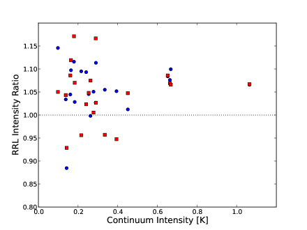
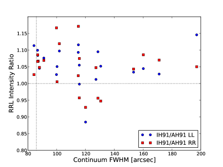
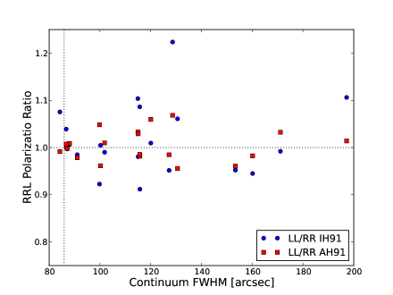
The electron temperature depends on the line-to-continuum ratio, therefore, in principle, we only require a relative intensity calibration. This is not true here since we have only measured the continuum at one frequency, near the ${\rm H}91\alpha$ RRL. Following Balser et al. (2011) we calculate an average RRL intensity relative to the ${\rm H}91\alpha$ line. The continuum data were taken at 8665$\,{\rm MHz}$ over a bandwidth that includes the ${\rm H}91\alpha$ transition, so we calibrated the Hn$\alpha$ lines relative to the ${\rm H}91\alpha$ line. In Figure 2, we plot the ratio of the interpolated ${\rm H}91\alpha$ intensity (IH91) and the average RRL intensity (AH91), scaled to the ${\rm H}91\alpha$ frequency as discussed above, for all 21 HRDS sources. The IH91/AH91 ratios are $1.058\pm\ 0.0533$ for LL and $1.048\pm\ 0.0631$ for RR. The ratios are offset by less than 5-10% from unity and are caused by errors in the noise tube calibration ($T_{\rm cal}$) and any systematic errors in our data reduction. The dispersion in IH91/AH91 may be caused by several factors that include systematic errors in the spectral baseline fits, random noise, elevation gain fluctuations, weather fluctuations, etc. The dispersion here is three times larger than in Balser et al. (2011) because the sources are weaker by more than a factor of 5. Nevertheless, we deem that the line-to-continuum calibration scale is accurate to within $\sim 5$%. Using these procedures we calculated and applied corrections factors of ${\rm CF}=1.058$ for LL and ${\rm CF}=1.048$ for RR.

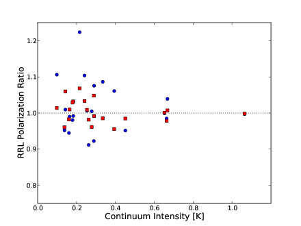
Comparing the RRL intensity for each polarization provides an additional check on our calibration. We derive polarization ratios of $1.016\pm\ 0.0714$ and $1.004\pm\ 0.0310$ for IH91 and AH91, respectively using all 21 HRDS sources (see Figure 3). These ratios are less than the expected $T_{\rm cal}$ uncertainties of about 10%. Moreover, the dispersion in the distribution from IH91 to AH91 decreases as $1/\sqrt{N}$ as expected for random Gaussian noise.

We used the IDL single-dish software package TMBIDL, written by our team, to analyze these data. The spectral line parameters were determined by first fitting the spectral baseline with a third-order polynomial, which was subtracted from the data, and then fitting Gaussian functions to the H, He, and C RRLs. Three parameters were derived for each RRL: the peak antenna temperature, the FWHM line width, and the Local Standard of Rest (LSR) velocity center. The continuum parameters were determined by first removing the background zero-level with a third-order polynomial and then using Gaussian functions to model the peak continuum intensity and the FWHM angular source size.

3 Results

Here we use radio observations of H ii regions to determine the metallicity structure of the Milky Way disk. Accurate measurement of the line-to-continuum ratio is necessary to derive the electron (thermal) temperature. Metals such as oxygen and nitrogen are the primary coolants in H ii regions and are well correlated with electron temperature (e.g., Shaver et al., 1983). Therefore we use the derived electron temperatures as a proxy for metallicity. H ii region locations are determined from the LSR velocity and a model of the rotation of the Galactic disk. Together these provide the information necessary to produce a map of the metallicity distribution in the Galactic disk.

Table 1 summarizes the RRL measurements for our 21 H ii region sample. Listed are the source name, the element, Gaussian fit parameters, the total integration time, the root-mean-square (rms) spectral noise, and the quality factor (hereafter QF; see below). The Gaussian fits include the peak intensity, the full-width at half-maximum (FWHM) line width, and the LSR velocity with their associated errors. The total integration time includes the average of both polarizations for the ${\rm H}87\alpha$, ${\rm H}88\alpha$, ${\rm H}89\alpha$, ${\rm H}91\alpha$, ${\rm H}92\alpha$, and ${\rm H}93\alpha$ transitions. Figure 4 shows sample spectra for three sources where the antenna temperature is plotted as a function of the LSR velocity. Since the H ii regions in our sample are distant, the peak intensities are weak, typically less than 50$\,{\rm mK}$. Helium and carbon RRLs are detected in fewer than 20% of the sample.

Table 2 summarizes the continuum measurements for this sample. Listed are the source name, Gaussian fit parameters to the continuum intensities in the R.A. and Decl. scan directions, the average Gaussian parameters, and the QF. The peak intensity and FWHM Gaussian fitted parameters are listed with their associated errors. The average peak intensity and FWHM correspond to the arithmetic and geometric mean, respectively. Figure 5 shows the continuum scans for the sources in Figure 4. The antenna temperature is plotted as a function of the offset R.A. and Decl. directions relative to the nominal source position.

The QF is a qualitative assessment of the line and continuum measurement where “A” is excellent and “D” is poor. Baseline structure and confusion are difficult to quantify and thus visual inspection is used to assess the quality of line and continuum data. Since the GBT RRL baselines are excellent with little line confusion at X-band, we follow Balser et al. (2011) and calculate the QF for the line data using the signal-to-noise ratio and the percent error of the Gaussian fit of the line area. For the continuum data the QF includes a visual assessment of the baseline structure, source confusion, the consistency of the peak intensity between the R.A. and Decl. scans, and the repeatability between the forward and backward scans. There are no QF=A sources for the RRL data since the signal-to-noise ratio is not sufficient for these more distant, weaker sources. Since our sample was selected based on the quality of the continuum data there are no QF=D sources for the continuum data.

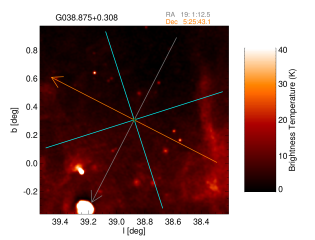
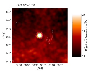
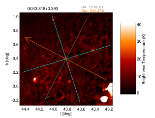
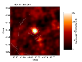
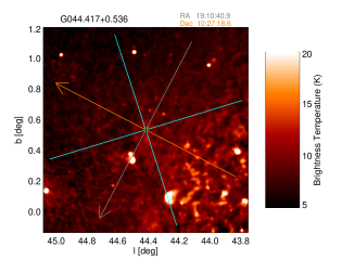
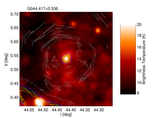
To better assess the level of source confusion we made crude 8.7$\,{\rm GHz}$ continuum images for each H ii region. This was accomplished with Spider continuum scans which consist of the R.A. and Decl. scans described above plus two additional pairs of scans rotated by 45$\,{}^{\circ}$ (see Robishaw & Heiles, 2009). There are 8 total scans for each Spider measurement that probe 4 cardinal directions both in the forward and backward direction. Figure 6 shows images produced from these Spider scans of the H ii regions in Figure 5. The 1.4$\,{\rm GHz}$ continuum emission from the VLA Galactic Plane Survey (VGPS Stil et al., 2006) is displayed by the color image. The orientation and extent of the Spider scans are shown as solid lines in the left panel. The central region is well sampled but there are large gaps in the outer regions where the data are interpolated. The right panel shows a magnified view of the central region with contours representing the GBT 8.7$\,{\rm GHz}$ continuum emission. Based on these Spider scan observations all of the H ii regions in our sample are clearly visible and reasonably well isolated from other sources.

3.1 Electron Temperature

For an optically thin nebula that is in local thermodynamic equilibrium (LTE), the hydrogenic RRL emission strength is proportional to $n_{\rm e}^{2}\,T_{\rm e}^{-2.5}$, whereas the thermal free-free continuum emission is proportional to $n_{\rm e}^{2}\,T_{\rm e}^{-1.35}$. Here $n_{\rm e}$ and $T_{\rm e}$ are the electron density and temperature, respectively. The line-to-continuum ratio is therefore proportional to $T_{\rm e}^{-1.15}$ and is an excellent probe of the electron (thermal) temperature of the ionized gas (Gordon & Sorochenko, 2009). Following Quireza et al. (2006), for RRLs near 9$\,{\rm GHz}$ the electron temperature is given by

$${\left(T_{\rm e}\over K\right)}=\left[7103.3{\left(\nu_{\rm L}\over{\rm GHz}\right)}^{1.1}\left({T_{\rm C}\over T_{\rm L}({\rm H{{}^{+}}})}\right){\left(\Delta V({\rm H{{}^{+}}})\over\,{\rm km\,s^{-1}}\right)}^{-1}\left(1+{y}\right)^{-1}\right]^{0.87}$$ (1)

where

$$y\equiv{n({{}^{4}}{\rm He}{{}^{+}})\over n({\rm H}{{}^{+}})}={{T_{L}({\rm{{}^{4}}He{{}^{+}}})\,\Delta V({\rm{{}^{4}}He{{}^{+}}})}\over{T_{L}({\rm H{{}^{+}}})\,\Delta V({\rm H{{}^{+}}})}},$$ (2)

and $\nu_{\rm L}$ is the H RRL rest frequency, $T_{\rm C}$ is the continuum peak intensity, $T_{\rm L}$ is the H (or He) RRL intensity, and $\Delta V$ is the H (or He) RRL FWHM line width. We use $\nu_{\rm L}=9$$\,{\rm GHz}$, the average H RRL frequency. Following Balser et al. (2011), we assume $y=0.08$ for sources with no detected helium emission. For typical H ii region electron densities and temperatures in our sample non-LTE effects and pressure broadening by electron impacts should be negligible at this frequency (c.f., Balser et al., 1999). Nevertheless, these effects on RRLs may introduce additional uncertainty into our analysis discussed in §3.3.

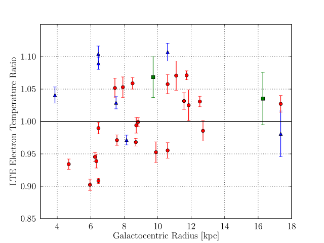
Table 3 lists values of $T_{\rm e}$ and $y$, together with other properties (see below), for the Green Bank sample. The RRL and continuum parameters together with the electron temperatures are derived using the same procedures and equations for all nebulae in the sample. The uncertainties are calculated by propagating the Gaussian fit errors through Equations 1 and 2. These random errors are typically less than 5%. We estimate systematic errors by comparing the results for sources observed twice by both the same telescope and different telescopes. Figure 7 plots the LTE electron temperature ratio as a function of the Galactic radius for these duplicate measurements. Shown are ratios for common sources within the GBT sample, the 140 Foot sample, and between the GBT and 140 Foot samples. We consider two sources to be the same if their positions are within the HPBW/2. When searching for GBT-140 Foot duplicates we use the larger 140 Foot HPBW/2 value. We only plot QFs between A–C. The rms of the electron temperature ratio for these duplicate measurements is 5%, larger than the random errors indicated by the error bars, but comparable to our calibration uncertainty.

3.2 H ii Region Distances

There are three main methods used to determine H ii region distances: geometrically (parallax), kinematically, and spectrophotometrically. Geometric distances are derived by measuring the parallax of molecular masers and associating them with H ii regions using position and radial velocity. They provide the most accurate distance measurement and are obviously preferred. There are 42 unique sources with parallax distances for the Green Bank sample. Distances determined using spectrophotometry can have lower formal errors than kinematic distances, but there are often large discrepancies between different studies. Moreover, many of our sources are optically obscured. Here, we only consider parallax and kinematic distances.

For consistency, we have redone the kinematic distance determination for all sources in the Green Bank sample following the procedures of Anderson et al. (2014). We use the Brand (1986) rotation curve model with two different sets of Galactic parameters: (1) a distance to the Galactic Center of $R_{\rm o}=8.5$$\,{\rm kpc}$ and a Solar circular rotation speed of $\Theta_{\rm o}=220$$\,{\rm km\,s^{-1}}$ (IAU parameters; hereafter, Kinematic-IAU); and (2) the parameters from Reid et al. (2014) where $R_{\rm o}=8.3$$\,{\rm kpc}$ and $\Theta_{\rm o}=240$$\,{\rm km\,s^{-1}}$ (hereafter, Kinematic-Reid). H ii regions in the inner Galaxy have a kinematic distance ambiguity (KDA). A KDA resolution (KDAR) was made using three methods: H i emission absorption (H i E/A), H₂CO absorption, and H i self-absorption (H i SA). Following Anderson et al. (2014) we employ these KDAR methods with the following priority: far distance H₂CO KDARs, H i E/A KDARs, H i SA KDARs, and near distance H₂CO KDARs.

Table 3 summarizes the H ii region properties of the Green Bank sample. Listed are the source name, the Galactic coordinates ($\ell,b$), the distance (${R_{\rm Sun}}$) and Galactocentric coordinates ($Az$, ${R_{\rm gal}}$), the helium abundance by number ($y$), the LTE electron temperature ($T_{\rm e}$), and the telescope used for the RRL and continuum observations. Three sets of (${R_{\rm Sun}}$, $Az$, ${R_{\rm gal}}$) are shown: Kinematic-IAU, Kinematic-Reid, and Best. The Best column gives values determined using parallax measurements when available, otherwise Kinematic-IAU parameters are used. Distances derived from parallax measurements are taken from the compilation in Reid et al. (2014).

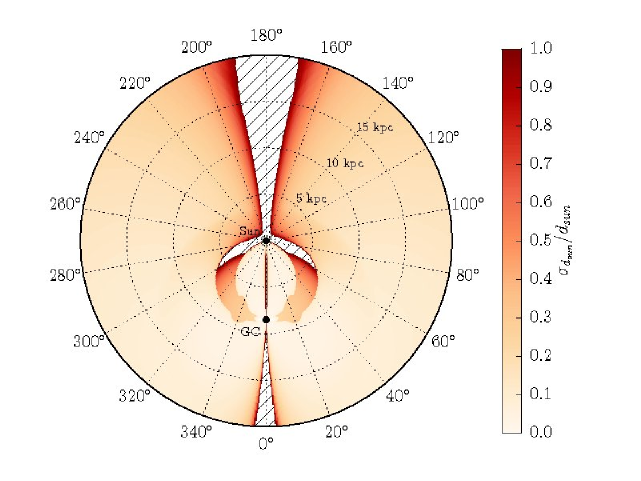
Kinematic distance uncertainties are estimated by exploring different rotation curves, streaming motions, and a change to the Solar circular rotation speed (Anderson et al., 2012). Figure 8 is a face-on Galactic plot of the fractional distance error from Wenger et al. (2015, in preparation). The largest errors occur when the radial velocity is small: toward the Galactic Center or anti-center and near the Sun. Distances are also not very well determined near the tangent point where the radial velocity is a maximum. This zone occupies a relatively small area.

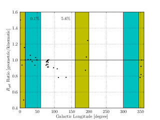
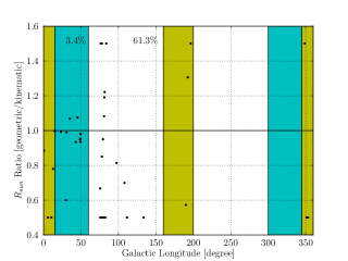
There are regions in the first and fourth quadrants, a zone that encompasses a large fraction of the Galactic disk, that have accurate (within $\sim\ 15$%) kinematic distances. Figure 9 plots ${R_{\rm gal}}$ and ${R_{\rm Sun}}$ ratios as a function of Galactic longitude for the Green Bank sample using geometric and kinematic methods. The Kinematic-IAU distances are used here for consistency of these comparisons. Values of ${R_{\rm gal}}$ derived using a kinematic model are typically within 5% of geometrically determined values, whereas there are significant deviations in ${R_{\rm Sun}}$ distances (Figure 9; also see Reid et al., 2014). The trends are similar when using the Kinematic-Reid distances. From Figures 8 and 9 it is clear that the largest kinematic distance uncertainties exist toward the Galactic Center and anti-center. We therefore remove any sources from our analysis that have longitudes with 15$\,{}^{\circ}$ of the Galactic Center or within 20$\,{}^{\circ}$ of the Galactic anti-center. These Galactic zones are indicated in Figure 9 by the green shaded region. The longitude zone with the lowest distance uncertainties, shown by the cyan shaded region in Figure 9, are between 15$\,{}^{\circ}$$-$60$\,{}^{\circ}$ in the first quadrant and 300$\,{}^{\circ}$$-$345$\,{}^{\circ}$ in the fourth quadrant. We measure an rms of 3.4% between the kinematic and parallax distances within this zone in the first quadrant. For the longitude zone that remains, encompassing most of the second and third quadrants, we measure an rms of 61.3%.

3.3 Electron Temperature Structure

H ii region electron temperatures are primarily set by the effective temperature of the ionizing star, the electron density of the surrounding medium, dust-particle interactions, and heavy elements (e.g., oxygen and nitrogen). H ii region models indicate that the metallicity is the dominant factor, where heavy elements within the ionized gas increase the cooling by the emission of collisionally excited lines (Rubin, 1985). Churchwell & Walmsley (1975) were the first to discover a positive radial electron temperature gradient in the Milky Way disk using RRLs. They interpreted this gradient as due to a negative radial metallicity gradient, where higher metal abundances at smaller radii produce lower electron temperatures. More recent RRL observations with the GBT revealed azimuthal electron temperature structure that may indicate the Galaxy is not well mixed at a given radius (Balser et al., 2011). Here we expand the H ii region sample using the HRDS to explore electron temperature structure over a larger area of the Galaxy.

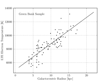
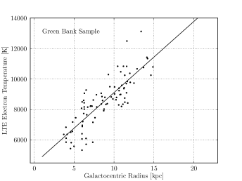
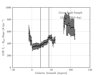
The electron temperature structure in the Galactic disk is derived for the three rotation curves: Kinematic-IAU (Figure 10), Kinematic-Reid (Figure 11), and Best distances (Figure 12). For this analysis we only include sources with distance errors less than 50%, QFs between A–C, and directions that exclude zones within 15$\,{}^{\circ}$ of the Galactic Center or within 20$\,{}^{\circ}$ of the Galactic anti-center. The gradient in electron temperature as a function of Galactic radius is defined by $T_{\rm e}=a+b\,R_{\rm gal}$, where $b$ is the “LTE $T_{\rm e}$–${R_{\rm gal}}$ slope”. Following Balser et al. (2011) we use the algorithm SLOPES to make ordinary least-squares fits (Isobe et al., 1990; Feigelson & Babu, 1992). In all cases we use jackknife resampling to derive more accurate uncertainties.

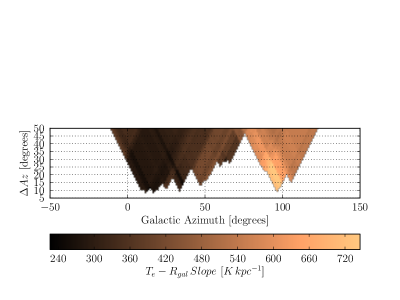
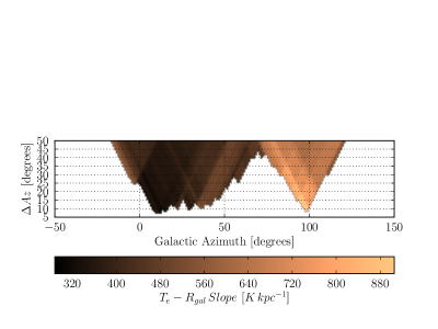
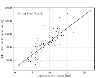
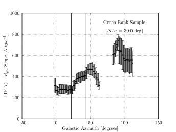
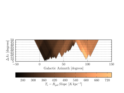
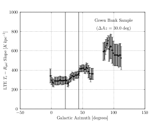
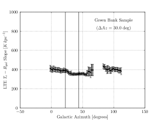
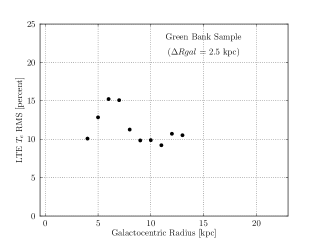
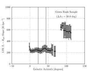
Each figure is comprised of four plots. The electron temperature as a function of Galactic radius is shown in the top left. The solid line is a fit to the data. The typical uncertainty for both $T_{\rm e}$ and ${R_{\rm gal}}$ is less than 5% (see Table 3). In the bottom left panel the electron temperature rms is plotted as a function of Galactic radius. The rms is calculated within $\Delta R_{\rm gal}=2.5$$\,{\rm kpc}$ bins that include 10 or more sources spanning 40$\,{}^{\circ}$ or more in azimuth. N.B., this requirement is not met for $R_{\rm gal}>14$$\,{\rm kpc}$ and therefore no data points are plotted for these radii. The rms scatter at specific ${R_{\rm gal}}$ values is larger than the typical $T_{\rm e}$ uncertainty of 5%, suggesting electron temperature azimuthal structure is present. The LTE $T_{\rm e}$–${R_{\rm gal}}$ slope as a function of azimuth is shown in the top right. Here we derive the slope within $\Delta{Az}=30$$\,{}^{\circ}$ bins that include 10 or more sources spanning an ${R_{\rm gal}}$ range larger than 10$\,{\rm kpc}$. The error bars are derived from SLOPES using jackknife resampling. The vertical solid lines mark the direction of the bar ($Az\sim 25$$\,{}^{\circ}$) and long bar ($Az\sim 45$$\,{}^{\circ}$) (Benjamin, 2008). The bottom right panel is a color map of the LTE $T_{\rm e}$–${R_{\rm gal}}$ slope as a function of both the azimuth bin size and azimuth. Here we explore different azimuth bin sizes to check if the bin size $\Delta{Az}=30$$\,{}^{\circ}$ is special in any way. Large bin sizes act to smooth variations in the LTE $T_{\rm e}$–${R_{\rm gal}}$ slope but provide more points in each bin and therefore better statistics. For the Kinematic-Reid analysis (Figure 11) we reduced the ${R_{\rm gal}}$ range constraint from 10$\,{\rm kpc}$ to 7$\,{\rm kpc}$ since the Galactic parameters adopted shrink the size of the Galactic disk.

Several trends are clear from these figures regardless of the distances used. There is a positive electron temperature radial gradient. This is well known and has been correlated with a radial metallicity gradient in the Galactic disk (see Shaver et al., 1983, and below). There is evidence for electron temperature azimuthal structure. Variations in $T_{\rm e}$ measured by the rms at a given Galactic radius are larger than the uncertainty. This is most significant near ${R_{\rm gal}}$ = 6$\,{\rm kpc}$. Azimuthal electron temperature structure is also revealed by variations in the LTE $T_{\rm e}$–${R_{\rm gal}}$ slope as a function of azimuth. The slope gradually increases from Galactic azimuth 0$\,{}^{\circ}$ to 60$\,{}^{\circ}$, but is almost a factor of two higher near $Az\sim 100$$\,{}^{\circ}$.

Balser et al. (2011) derived LTE $T_{\rm e}$–${R_{\rm gal}}$ slopes of $392\pm\ 84$$\rm\,K\,kpc^{-1}$, $228\pm\ 26$$\rm\,K\,kpc^{-1}$, and $404\pm\ 42$$\rm\,K\,kpc^{-1}$ between azimuth zones of $330$$\,{}^{\circ}$$-360$$\,{}^{\circ}$, $0$$\,{}^{\circ}$$-30$$\,{}^{\circ}$, and $30$$\,{}^{\circ}$$-60$$\,{}^{\circ}$, respectively. Here we have discarded many H ii regions between $Az=330$$\,{}^{\circ}$$-360$$\,{}^{\circ}$ because of large distance uncertainties and therefore do not plot these. For Figure 10, we derive slopes of $297\pm\ 41$$\rm\,K\,kpc^{-1}$and $384\pm\ 42$$\rm\,K\,kpc^{-1}$ for azimuth zones $0$$\,{}^{\circ}$$-30$$\,{}^{\circ}$ and $30$$\,{}^{\circ}$$-60$$\,{}^{\circ}$, respectively. For the analysis here, the trend is the same but the amplitude of these $T_{\rm e}$ variations is less. The new HRDS sources populate $90$$\,{}^{\circ}$$-130$$\,{}^{\circ}$ where we calculate a slope of $551\pm\ 92$$\rm\,K\,kpc^{-1}$, significantly larger than those at lower azimuths.

There are some differences between the three analyses explored here. The Kinematic-Reid distances shrink the overall size of the Galactic disk and this increases the LTE $T_{\rm e}$–${R_{\rm gal}}$ slopes by about 20%. The LTE $T_{\rm e}$ rms peaks near $R_{\rm gal}=6$$\,{\rm kpc}$ for all analyses, but the value is 30% higher for the Best distances compared with Kinematic-IAU or Kinematic-Reid. We do not know whether this is real or due to some yet to be identified source of systematic uncertainty.

Our H ii regions are not uniformly distributed in the Galactic plane (see Figure 1). Could this non-uniform distribution produce azimuthal electron temperature structure where none exists? We explore such a possibility by randomly generating the electron temperatures for each H ii region location in our sample and assuming that only a radial $T_{\rm e}$ gradient exits. We assume $T_{\rm e}=a+b\,R_{\rm gal}$, where $a=4928\pm\ 277$$\,{\rm K}$ and $b=385\pm\ 29$$\rm\,K\,kpc^{-1}$. The values for $a$ and $b$ are taken from the fits to the Green Bank sample using the Kinematic-IAU distances. We perform this experiment 100 times. The middle panels in Figure 13 show a typical result. We plot the LTE $T_{\rm e}$ rms as a function of Galactic radius (left) and the LTE $T_{\rm e}$–${R_{\rm gal}}$ slope as a function of azimuth (right). For comparison we show the results from Figure 10 in the top two panels. The LTE $T_{\rm e}$ rms values are around 5% for our experiment, consistent with uncertainties in the electron temperature. The LTE $T_{\rm e}$–${R_{\rm gal}}$ slope is approximately constant around 400$\rm\,K\,kpc^{-1}$ with no significant variations with azimuth. We calculate a mean LTE $T_{\rm e}$–${R_{\rm gal}}$ slope over the 100 random experiments of $386\pm\ 15$$\rm\,K\,kpc^{-1}$ and $384\pm\ 34$$\rm\,K\,kpc^{-1}$ for $Az=0$$\,{}^{\circ}$$-60$$\,{}^{\circ}$ and $Az=90$$\,{}^{\circ}$$-130$$\,{}^{\circ}$, respectively. We therefore conclude that the non-uniform H ii region distribution of our sample cannot artificially produce azimuthal metallicity structure.

For most of the H ii regions in our sample we must rely on kinematic distances (${R_{\rm Sun}}$). For some Galactic locations, kinematic distances uncertainties can be larger than 50% (see §3.2). How do these uncertainties affect electron temperature structure within the Galactic disk? Could these uncertainties be artificially producing the observed electron temperature structure? The uncertainties for ${R_{\rm gal}}$ are typically less than 5% and when combined in quadrature with the 5% error in $T_{\rm e}$ should produce radial electron temperature gradients with an accuracy of better than 10%. But determining Galactic azimuth requires ${R_{\rm Sun}}$, and therefore azimuthal electron temperature structure has larger uncertainties.

To explore how kinematic distance uncertainties affect our results we perform Monte Carlo simulations using the Kinematic-IAU distances for the Green Bank sample. We assume the errors in $T_{\rm e}$ and ${R_{\rm Sun}}$ have a Gaussian distribution. For each simulation we modify the values of $T_{\rm e}$ and ${R_{\rm Sun}}$ by adding randomly generated, Gaussian errors to each source. For $T_{\rm e}$ we use a Gaussian FWHM of 5%, the rms value derived from the Figure 7 data. For ${R_{\rm Sun}}$ we use a Gaussian FWHM of 3.4% for $15<\ell<60$$\,{}^{\circ}$ and 61% for $61<\ell<160$$\,{}^{\circ}$ based on the results in Figure 9. We then propagate these new ${R_{\rm Sun}}$ values to $Az$ and ${R_{\rm gal}}$. We ran 100 Monte Carlo simulations. The bottom panel in Figure 13 shows typical results for one simulation. The variations in the LTE $T_{\rm e}$–${R_{\rm gal}}$ slope between $Az=0$$\,{}^{\circ}$$-60$$\,{}^{\circ}$ have been significantly reduced, producing a constant slope to within the rms of the fits. The much larger gradients near $Az\sim\ 100$$\,{}^{\circ}$, however, remain for most simulations. We calculate a mean LTE $T_{\rm e}$–${R_{\rm gal}}$ slope over the 100 Monte Carlo simulations of $246\pm\ 28$$\rm\,K\,kpc^{-1}$ and $507\pm\ 79$$\rm\,K\,kpc^{-1}$ for $Az=0$$\,{}^{\circ}$$-60$$\,{}^{\circ}$ and $Az=90$$\,{}^{\circ}$$-130$$\,{}^{\circ}$, respectively.

We conclude that the azimuthal electron temperature structure over $Az=0$$\,{}^{\circ}$$-60$$\,{}^{\circ}$ detected by Balser et al. (2011), and confirmed here, is not statistically significant. This is due to the large kinematic distance uncertainties in this azimuth zone (see Figure 8). The much higher LTE $T_{\rm e}$–${R_{\rm gal}}$ slopes between $Az=90$$\,{}^{\circ}$$-130$$\,{}^{\circ}$, however, appear to be significant and indicate real azimuthal electron temperature structure. Table 4 summarizes these results where the average LTE $T_{\rm e}$-${R_{\rm gal}}$ slope is given, over these two azimuth ranges, for the Kinematic-IAU data and the two simulations described above.

3.4 O/H Abundance Ratio

Churchwell & Walmsley (1975) were the first to suggest that the radial electron temperature gradient observed in the Milky Way is a result of an abundance gradient of heavy elements. Using CELs from oxygen at optical wavelengths along with electron temperatures from RRLs, Shaver et al. (1983) derived a relationship between Log(O/H) and $T_{\rm e}$:

$$[{\rm O/H}]\equiv 12+{\rm Log(O/H)}=(9.82\pm 0.02)-(1.49\pm 0.11)\,T_{\rm e}/10^{4}\,{\rm K}.$$ (3)

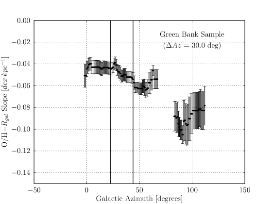
More recently, Afflerbach et al. (1996, 1997) observed higher frequency RRLs and far IR CELs toward a sample of ultracompact (UC) H ii regions to derive radial abundance gradients. These data have several advantages compared to Shaver et al. (1983): the RRLs have higher signal-to-noise ratios; the higher frequency RRLs are less likely to suffer from non-LTE effects; and the far IR lines are less susceptible to extinction by dust. In principle we could use the Afflerbach et al. results to derive O/H abundances from our $T_{\rm e}$ values. The higher electron densities in UC H ii regions, however, increase $T_{\rm e}$ by $\sim 1000$$\,{\rm K}$ compared to the classical H ii regions observed by Shaver et al. (1983) and that are typical of our sample (Rubin, 1985; Afflerbach et al., 1996). Therefore, following Balser et al. (2011) we use Equation 3 to calculate [O/H] abundances across the Galactic disk. Since this is a linear relationship, the electron temperature structure discussed in §3.3 will pertain to the [O/H] abundance ratio, except that the radial gradient will be negative with [O/H] decreasing with Galactic radius. We define the gradient in [O/H] as a function of Galactic radius by $[{\rm O/H}]=c+d\,R_{\rm gal}$, where $d$ is the “[O/H]–${R_{\rm gal}}$ slope”. Figure 14 plots the [O/H]–${R_{\rm gal}}$ slope as a function of Galactic azimuth. The [O/H]–${R_{\rm gal}}$ slope increases from around $[{\rm O/H}]\sim-0.04$ between $Az=0$$\,{}^{\circ}$$-60$$\,{}^{\circ}$ to $[{\rm O/H}]\sim-0.08$ between $Az=90$$\,{}^{\circ}$$-130$$\,{}^{\circ}$.

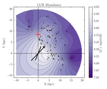
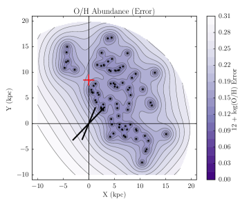
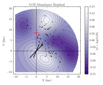
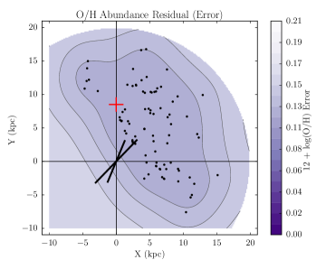
We use the software package pyKrige, which employs Kriging (see Feigelson & Babu, 2012), to interpolate the distribution of [O/H] abundances from the Green Bank sample of H ii regions to produce an image (Figure 15). The [O/H] values near the Sun are similar to the solar value of $8.69\pm\ 0.05$ (Asplund et al., 2009). Therefore, both the $T_{\rm e}$–[O/H] calibration from Shaver et al. and our derived electron temperatures are consistent with Solar measurements. The negative [O/H] radial gradient is evident with larger abundances near the Galactic center. We find that $[{\rm O/H}]=(9.086\pm\ 0.041)+(-0.0573\pm\ 0.0043)\,R_{\rm gal}$ using the Green Bank sample. This radial gradient slope is consistent, to within the uncertainties, with Afflerbach et al. (1997). We produce an [O/H] residual image by subtracting this fit from the data (Figure 16). The [O/H] residuals span about 0.3 dex. The residuals are smaller along the direction of the long bar, oriented toward $Az=44\pm\ 10$$\,{}^{\circ}$ (Benjamin, 2008).

4 Discussion

The most prominent metallicity structure in the Milky Way disk is the decrease of metallicity with increasing Galactic radius—the radial metallicity gradient. All of the major tracers reveal radial gradients, typically with slopes between $-0.03$ to $-0.09$$\rm\,dex\,kpc^{-1}$. The radial metallicity gradient can be explained by an inside-out galaxy formation where the disk grows via a radially dependent gas infall rate and star formation rate (e.g., Matteucci & François, 1989). But why is there such a wide range of radial gradient slopes measured? There are several possibilities. (1) Measurement uncertainty. Measurement errors will cause some variations, but it is unlikely to produce a factor of three difference in slope. Homogeneity in observing procedures and data analysis may be more important given the variations in abundance that can be derived for the same source (for further discussion see Rudolph et al., 2006; Henry et al., 2010; Balser et al., 2011). (2) Dynamical evolution. Radial gradients calculated with stellar tracers may be affected by radial migration, where stars are scattered into different orbits (Sellwood & Binney, 2002). Radial migration should flatten the radial metallicity gradient, but there is some evidence that this may not be a large factor for stars in the Milky Way (Di Matteo et al., 2013; Kubryk et al., 2013; Bovy et al., 2014). (3) Temporal evolution. Many tracers have a wide range of age and therefore are probing the Milky Way disk at different times. For example, the radial gradient has been observed to flatten with time when using Open clusters (e.g., Friel et al., 2002). But accurate ages are crucial to separate out these temporal effects. Planetary nebulae (PNe) studies indicate a flattening of the radial gradient with time (Maciel et al., 2003), a steepening with time (Stanghellini & Haywood, 2010), or no temporal variation (Henry et al., 2010). These vastly different conclusions reveal the difficulty in deriving accurate PNe ages and distances. (4) Sample Evolution. Hayden et al. (2013) measure a flattening of the radial gradient away from the Galactic mid-plane. Therefore, including sources out of the Galactic plane, which may be from an older population, may alter the derived radial gradient slope (see Minchev et al., 2014). Azimuthal abundance variations have been reported (e.g., Pedicelli et al., 2009; Balser et al., 2011, §3.3). If real, these will complicate any analysis of radial gradients. Here we detect metallicity gradient slopes over different azimuth ranges that span the values observed in the literature. The usual assumption is that the disk is well mixed at a given radius but this may not be true.

Twarog et al. (1997) were the first to measure a break in the radial gradient around 10$\,{\rm kpc}$, and a flattening at larger radii. We detect no such flattening here. Balser et al. (2011) suggested that many of the studies showing breaks in the radial gradient use heterogeneous data sets, or that the flattening disappears when restricting sources to be near the mid-plane. Abundance studies in external disk galaxies, however, detect a flattening of the radial gradient beyond twice the effective radius, the radius that contains half the total light (e.g., Bresolin et al., 2009, 2012; Marino et al., 2012). Pilyugin (2003) suggested that a flattening could be artificially produced by using the strong line method (e.g., $R_{23}$) to derive the [O/H] abundance ratio. But there are examples where the more accurate direct method, involving the [O III]$\lambda$4363 auroral line, was used to derive the [O/H] abundance ratio and the flattening persists (e.g., Bresolin et al., 2009).

Explanations for the flattening include variations in gas density, the presence of a bar (e.g., radial migration), the corotation resonance (the radius where the rotation speed of the spiral arm equals that of the material in the disk), and mergers. Sánchez et al. (2014) measured the oxygen abundance radial gradient in the disks of 306 galaxies using H ii regions. They find a slope that is independent of morphology, the presence of bars, absolute magnitude, or mass; but the gradient is flatter for interacting galaxies. Most galaxies with sufficient data indicate a flattening of the gradient beyond two effective radii. Sánchez et al. (2014) attribute this flattening to secular evolution (e.g., radial migration or mergers). Scarano & Lépine (2013) analyzed the metallicity gradient and the corotation radius in 16 galaxies. They find a correlation between the corotation radius and the radius where there exists a metallicity break in the radial gradient for most galaxies. Nevertheless, the empirical evidence for any radial break in the metallicity is not clear in the Milky Way.

Azimuthal metallicity structure has been claimed by some authors. Observations of Cepheids indicate metallicity variations across Galactic quadrants II and III near ${R_{\rm gal}}$ $\approx 10$$\,{\rm kpc}$ (Luck et al., 2006; Lemasle et al., 2008; Pedicelli et al., 2009). More recently, however, Genovali et al. (2014) find that these azimuthal residuals are correlated with candidate Cepheid groups. These are spatial overdensities of Cepheids related to star clusters, and they may be responsible for the observed variations (also see Luck & Lambert, 2011). Balser et al. (2011) detected similar metallicity structure using H ii regions, along with variations in the radial gradient with Galactic azimuth between $Az=330-60$$\,{}^{\circ}$. Here we determine kinematic distances for all sources in a consistent way and use Monte Carlo simulations to assess how distance uncertainties will effect our results. Although we detect the same azimuthal metallicity structure as Balser et al. (2011), we conclude that this structure is not statistically significant because of the large kinematic distance uncertainties between $Az=330-60$$\,{}^{\circ}$. Nevertheless, the doubling of the [O/H]–${R_{\rm gal}}$ slope from $Az=0$$\,{}^{\circ}$$-60$$\,{}^{\circ}$ to $Az=90$$\,{}^{\circ}$$-130$$\,{}^{\circ}$ is statistically significant (see Figure 14). The [O/H]–${R_{\rm gal}}$ slope increases from around $[{\rm O/H}]\sim-0.04$ between $Az=0$$\,{}^{\circ}$$-60$$\,{}^{\circ}$ to $[{\rm O/H}]\sim-0.08$ between $Az=90$$\,{}^{\circ}$$-130$$\,{}^{\circ}$.

Measuring radial gradients requires accurate determination of the Galactic radius (${R_{\rm gal}}$), whereas probing azimuthal structure depends on the distance from the Sun, ${R_{\rm Sun}}$. Figure 9 shows that the kinematic method is able to determine accurate ${R_{\rm gal}}$ values for most of the Galaxy. Determining accurate ${R_{\rm Sun}}$ distances, however, is much more difficult. This problem is avoided for extragalactic objects where relative locations within the disk are easier to determine. Some authors have claimed azimuthal metallicity variations in extragalactic sources; for example, in the nearby spiral galaxies M31 (Sanders et al., 2012), M33 (Rosolowsky & Simon, 2008), and M101 (Kennicutt & Garnett, 1996). But when the more accurate direct method is used to derive the [O/H] abundance ratio, non-radial metallicity structure is not detected: M31 (Zurita & Bresolin, 2012), M33 (Bresolin, 2011), and M101 (Li et al., 2013). Unlike the Milky Way these galaxies do not contain a bar.

Galactic chemical evolution (GCE) models have become more complex over the last decade. Early GCE models divided the disk into annuli with no radial exchange of material, and typically employed a Schmidt-Kennicutt star formation law that included infalling gas (e.g., Chiappini et al., 1997). These models can generally reproduce the observed radial metallicity gradient but they include free parameters that can be tuned to match the observations. It has been known for many years that non-axisymmetric forces, such as spiral arms, can change the angular momentum of stars in the Galaxy (Barbanis & Woltjer, 1967). Sellwood & Binney (2002) showed that the dominant effect of spiral arms is the resonant scattering of stars located at corotation; stars can therefore migrate radially while maintaining a circular orbit.

Chemodynamical models consider both the chemical and dynamical evolution of the Galaxy (e.g., Samland et al., 1997; Schönrich & Binney, 2009; Kubryk et al., 2013; Minchev et al., 2014). They produce radial metallicity gradients that are within the range observed, but, as discussed above, the derived gradient slopes vary by a factor of three between the different studies and is therefore not well constrained. Kubryk et al. (2013) considered the chemical evolution of both the stars and gas in a bar dominated disk galaxy. There are no azimuthal variations in either the stars or gas at early times, but at late times (10$\,{\rm Gyr}$) the corotation of the bar moves outward allowing metal poor gas to flow inward creating azimuthal variations up to a factor of two in the gas in the outer regions (${R_{\rm gal}}$= 12$\,{\rm kpc}$). This may explain the lower radial metallicity gradients we observe in the direction of the bar. Since most of the stars have already been formed at all radii before radial gas flows are induced by the bar, stars show little azimuthal metallicity structure in these simulations (also see Di Matteo et al., 2013). This is consistent with metallicity measurements of red clump stars in the Galaxy (Bovy et al., 2014). One caveat is that these simulations do not include infall, which could also create azimuthal variations.

5 Summary

We measure the RRL and continuum emission with the GBT toward 21 Galactic H ii regions between Galactic azimuth $Az=90-130$$\,{}^{\circ}$ at X-band ($8-10\,$$\,{\rm GHz}$). We derive electron temperatures from the line-to-continuum ratio assuming LTE, and use the $T_{\rm e}$–[O/H] calibration from Shaver et al. (1983) to determine the metallicity. We combine these results with our previous efforts using the NRAO 140 Foot (Quireza et al., 2006) and GBT (Balser et al., 2011) to produce a high quality sample of 90 sources over $Az=0-130$$\,{}^{\circ}$, spanning Galactic radii ${R_{\rm gal}}$ = $4-17$$\,{\rm kpc}$.

We find radial metallicity gradients, [O/H] vs ${R_{\rm gal}}$, between $-0.04$ and $-0.08$$\rm\,dex\,kpc^{-1}$ depending on the azimuth range sampled. We see no evidence for a break or flattening of the radial gradient near ${R_{\rm gal}}$ = 10$\,{\rm kpc}$. We confirm the azimuthal metallicity structure detected by Balser et al. (2011) between $Az=0-60$$\,{}^{\circ}$, but the magnitude of the metallicity variations is reduced by 25%. Monte Carlo simulations, however, indicate that the azimuthal metallicity structure in this azimuth zone is not statistically significant. Nevertheless, the large variations in the [O/H]–${R_{\rm gal}}$ slope, by almost a factor of two, between azimuth zone $Az=0$$\,{}^{\circ}$$-60$$\,{}^{\circ}$and $Az=90$$\,{}^{\circ}$$-130$$\,{}^{\circ}$ is significant. We suggest that the lower radial metallicity gradients over $Az=0-60$$\,{}^{\circ}$ may be the result of radial mixing from the bar.

Determining metallicity structure using RRLs in H ii regions has many advantages. H ii regions are very young and probe metallicity at the current epoch—there is no need to correct for age. They are not influenced by dynamical effects such as radial migration. RRLs can probe H ii regions across the Galactic disk and therefore provide a more comprehensive view of chemical evolution. There are, however, two main drawbacks. First, the method of deriving metallicities is indirect; we calculate electron temperature and determine [O/H] abundances derived from optical data. We plan to update this calibration using better optical data and IR data from Herschel, along with H ii region models using the program Cloudy to better understand the calibration. Second, kinematic distances are used to determine the H ii region locations and can have large errors. But many sources now have very accurate distances determined from maser parallax measurements. As reported here we have a much better understanding of the quality of our kinematic distances. Future parallax measurements will improve the situation.

Figure 1: Galactic distribution of H ii regions in the Green Bank sample. Plotted are the Galactic location ($Az,R_{\rm gal}$) of H ii regions from Quireza et al. (2006) (black crosses) and Balser et al. (2011) (black circles). The HRDS H ii regions studied here are shown as red circles. The blue circle marks the location of the Sun 8.5$\,{\rm kpc}$ from the Galactic Center, which lies at the plot origin.

Figure 2: RRL intensity ratios as a function of continuum intensity (top) and FWHM angular size (bottom). Three different ${\rm H}91\alpha$ intensities are calculated for all sources: H91 is the ${\rm H}91\alpha$ intensity; IH91 is the ${\rm H}91\alpha$ intensity measured after the velocity scale has been interpolated; and AH91 is the ${\rm H}91\alpha$ intensity after the six adjacent RRLs have been interpolated and averaged. Plotted are IH91/AH91 for each polarization. The horizontal dashed line is a ratio of unity, whereas the vertical dashed line is the GBT’s HPBW at 8.7$\,{\rm GHz}$. We find that the IH91/AH91 ratios are typically less than 5-10% from unity and are not correlated with either continuum intensity or angular size.

Figure 3: RRL polarization ratios as a function of continuum intensity (top) and FWHM angular size (bottom). Plotted are the polarization ratios (LL/RR) for the IH91 and AH91 RRL intensities (see Figure 2). The AH91 polarization ratios are consistent with random errors in $T_{\rm cal}$.

Figure 4: Sample H ii region RRL spectra. The antenna temperature is plotted as a function of the LSR velocity. The LSR velocity is referenced with respect to the H89$\alpha$ RRL. For some sources the He and C RRLs, located about $-125$$\,{\rm km\,s^{-1}}$ from the H line, are detected. The bottom right hand plot duplicates the spectrum for G044.417+0.536 where we smooth the spectrum to 2.61$\,{\rm km\,s^{-1}}$ to reveal the narrow carbon RRL. A third order polynomial function is fit to the line free regions and removed from the data. The quality factor is shown at the top right-hand corner of each plot, where QF=A is excellent and QF=D is poor.

Figure 5: Sample H ii region continuum scans. The antenna temperature is plotted as a function of the offset position relative to the target coordinates. For each source the R.A. and Decl. scans are shown. A third order polynomial function is fit to the baseline and removed from the data. The quality factor is shown at the top right-hand corner of each plot, where QF=A is excellent and QF=D is poor.

Figure 6: Sample H ii region continuum images in Galactic coordinates. Left panel: 1.4$\,{\rm GHz}$ VGPS continuum image (80$\,{}^{\circ}$ $\times$ 80$\,{}^{\circ}$) with the Spider scan orientation and extent shown as solid lines. Increasing R.A. and Decl. directions are indicated by the arrows. The R.A. and Decl. coordinates of the center of the map are shown at the top right corner of the plot. Right panel: 1.4$\,{\rm GHz}$ VGPS continuum image (20$\,{}^{\circ}$ $\times$ 20$\,{}^{\circ}$) with contours from the 8.7$\,{\rm GHz}$ GBT continuum, interpolated from the Spider scan data. The green circle at the center of the image indicates the size of the GBT HPBW. Contour levels range from 0.1 to 0.9 of the peak in increments of 0.1.

Figure 7: LTE electron temperature comparison. Plotted is the electron temperature ratio as a function of Galactic radius for sources in common with the GBT (green squares), the 140 Foot (blue triangles), and with the GBT and 140 Foot samples (red circles). Only sources with QF A, B, or C are included.

Figure 8: Face-on Galactic map of distance uncertainties from Wenger et al. (2015, in preparation) based on the analysis of Anderson et al. (2014). The distance uncertainties were calculated by exploring different rotation curves, streaming motions, and a change to the Solar circular rotation speed. Shown are the fractional distance uncertainties. The hatched regions have fractional uncertainties larger than unity.

Figure 9: Comparison of parallax distances with kinematic distances as a function of Galactic longitude. The Kinematic-IAU values are used for consistency. Left: Galactic distance ratio (${R_{\rm gal}}$). Right: Solar distance ratio (${R_{\rm Sun}}$). The green regions are within 15$\,{}^{\circ}$ of the Galactic Center or 20$\,{}^{\circ}$ of the Galactic anti-center. Kinematic distances are not very reliable over these longitudes since the radial velocity from Galactic rotation is near zero for all distances. The cyan regions are between $15-60$$\,{}^{\circ}$ in the first Galactic quadrant or between $300-345$$\,{}^{\circ}$ in the fourth Galactic quadrant. In this longitude zone we derive a median percent difference between the kinematic and geometric methods of 0.1% and 3.4% for ${R_{\rm gal}}$ and ${R_{\rm Sun}}$, respectively. The remaining longitude range, shown in white, has larger kinematic distance uncertainties with a median percent difference of 5.6% and 61.3% for ${R_{\rm gal}}$ and ${R_{\rm Sun}}$. respectively. These median percent difference numbers are shown at the top of each plot. Ratio values are truncated to be between 0.5 and 1.5 for clarity.

Figure 10: Electron temperature structure using Kinematic-IAU distances for the Green Bank sample. Top left: LTE electron temperature as a function of Galactic radius. The points are data and the solid line is a fit to these data with $T_{\rm e}=(4928\pm\ 277)+(385\pm\ 29)\,R_{\rm gal}$. Errors bars are not included for clarity. Bottom left: LTE electron temperature rms within Galactic radius bins of $\Delta R_{\rm gal}=2.5$$\,{\rm kpc}$. The electron temperature uncertainty is $\sim 5$%. Only bins that include 10 or more sources spanning 40$\,{}^{\circ}$ or more in azimuth are plotted. This requirement is not met for $R_{\rm gal}>14$$\,{\rm kpc}$ and therefore no data points are plotted for these radii. Top right: LTE $T_{\rm e}$–${R_{\rm gal}}$ slope as a function of azimuth. Azimuth bin sizes of $\Delta{Az}=30$$\,{}^{\circ}$ are centered at the indicated azimuth. The error bars are derived using the SLOPES algorithm with jackknife resampling. Only bins that include 10 or more sources spanning an ${R_{\rm gal}}$ range larger than 10$\,{\rm kpc}$ are shown. These requirements are not met for $Az\sim\ 75$$\,{}^{\circ}$ which explains the gap in data points near this azimuth. The vertical solid lines mark the orientation of the bar ($Az\sim 25$$\,{}^{\circ}$) and long bar ($Az\sim 45$$\,{}^{\circ}$) (Benjamin, 2008). Bottom right: LTE $T_{\rm e}$–${R_{\rm gal}}$ slope color map as a function of bin size ($\Delta{Az}$) and azimuth ($Az$). Here we explore the effects of using different bin sizes.

Figure 11: Electron temperature structure using Kinematic-Reid distances for the Green Bank sample. See Figure 10 for details. The fit to the data in the top left plot is $T_{\rm e}=(4446\pm\ 301)+(467\pm\ 34)\,R_{\rm gal}$.

Figure 12: Electron temperature structure using Best distances for the Green Bank sample. See Figure 10 for details. The fit to the data in the top left plot is $T_{\rm e}=(4821\pm\ 328)+(402\pm\ 33)\,R_{\rm gal}$.

Figure 13: Monte Carlo simulations of the electron temperature and kinematic distance uncertainties. The Kinematic-IAU distances are used for the Green Bank sample. Left: LTE electron temperature rms as a function of Galactic radius. Right: LTE $T_{\rm e}$–${R_{\rm gal}}$ slope as a function of Galactic azimuth. Top: same plots as shown in Figure 10 for comparison. Middle: results from randomly generating the electron temperatures assuming $T_{\rm e}=a+b\,R_{\rm gal}$. The values for $a$ and $b$ are taken from the fits to the Green Bank sample using the Kinematic-IAU distances. Bottom: results from a Monte Carlo simulation that randomly adds Gaussian uncertainties to the $T_{\rm e}$ and the Galactic position (see text).

Figure 14: [O/H]–${R_{\rm gal}}$ slope as a function of Galactic azimuth using the Kinematic-IAU distances. Azimuth bin sizes of $\Delta{Az}=30$$\,{}^{\circ}$ are centered at the indicated azimuth. The error bars are the uncertainties calculated by the SLOPES algorithm using jackknife resampling. The vertical solid lines mark the orientation of the bar ($Az\sim 25$$\,{}^{\circ}$) and long bar ($Az\sim 45$$\,{}^{\circ}$) (Benjamin, 2008).

Figure 15: Face-on Galactic [O/H] abundance ratio image using Kriging to interpolate between the discrete H ii region values (left), and the corresponding $1\sigma$ errors (right). A power law variogram model produced the best fit. The points indicate the location of the discrete H ii regions. The solid lines intersect at the Galactic Center. The red lines mark the location of the Sun. The thick lines correspond to the central locii of the putative “short” and “long” bars (Benjamin, 2008). The very low abundance near ($Az=97.7$$\,{}^{\circ}$, ${R_{\rm gal}}$ = 15.3$\,{\rm kpc}$) is dominated by G55.11+2.4 (S83) (Balser et al., 2011). This H ii region has a continuum QF = A and a spectral line QF = B, and therefore we have no reason to exclude it in our analysis.

Figure 16: Face-on Galactic [O/H] abundance residual image using Kriging to interpolate between the discrete H ii region values (left), and the corresponding $1\sigma$ errors (right). A Gaussian variogram model produced the best fit. (See Figure 15.)

Table 1: Radio Recombination Line Parameters of Galactic H ii Regions

		$T_{\rm L}$	$\sigma\,T_{\rm L}$	$\Delta{V}$	$\sigma\,\Delta{V}$	$V_{\rm LSR}$	$\sigma\,V_{\rm LSR}$	$t_{\rm intg}$	rms
Name	Element	(mK)	(mK)	($\,{\rm km\,s^{-1}}$)	($\,{\rm km\,s^{-1}}$)	($\,{\rm km\,s^{-1}}$)	($\,{\rm km\,s^{-1}}$)	(hr)	(mK)	QF
G027.562+0.084	H	40.63	0.47	21.63	0.29	$87.16$	0.12	11.1	2.40	C
G031.274+0.485	H	9.30	0.33	23.20	0.99	$-6.49$	0.40	23.8	1.86	D
G032.272-0.226	H	59.00	0.40	25.83	0.20	$21.14$	0.09	11.9	2.26	B
	He	8.35	0.49	17.15	1.17	$19.70$	0.50	$\cdots$	$\cdots$	$\cdots$
	C	6.21	0.88	5.32	0.88	$20.70$	0.37	$\cdots$	$\cdots$	$\cdots$
G032.733+0.209	H	22.63	0.40	21.04	0.44	$16.16$	0.18	19.0	2.14	C
G032.876-0.423	H	29.27	0.60	18.17	0.43	$49.56$	0.18	9.5	2.75	C
G032.928+0.607	H	44.37	0.37	27.40	0.27	$-38.49$	0.11	14.3	2.23	C
	He	3.33	0.33	36.07	4.66	$-45.03$	1.92	$\cdots$	$\cdots$	$\cdots$
	C	5.72	1.31	2.34	0.64	$-36.99$	0.26	$\cdots$	$\cdots$	$\cdots$
G032.976-0.334	H	27.22	0.61	20.90	0.54	$49.60$	0.23	9.5	2.90	C
G034.041+0.053	H	36.38	0.53	23.72	0.40	$36.52$	0.17	11.5	2.55	C
G034.133+0.471	H	108.65	0.50	25.29	0.13	$34.19$	0.06	8.3	2.80	B
	He	8.15	0.56	20.00	1.59	$35.24$	0.67	$\cdots$	$\cdots$	$\cdots$
G034.686+0.068	H	41.52	0.60	25.69	0.44	$51.87$	0.18	9.1	2.82	C
G037.755+0.560	H	19.22	0.42	23.37	0.75	$17.90$	0.28	16.5	2.02	C
G038.550+0.163	H	29.26	0.43	23.16	0.40	$25.70$	0.17	10.3	2.57	C
G038.651+0.087	H	17.80	0.33	26.98	0.60	$-40.52$	0.25	19.0	2.01	C
G038.840+0.497	H	13.19	0.32	27.82	0.80	$-43.29$	0.33	18.6	2.04	D
G038.875+0.308	H	54.86	0.45	28.46	0.27	$-14.79$	0.11	9.5	2.64	B
	He	4.83	0.57	17.19	2.35	$-14.21$	1.00	$\cdots$	$\cdots$	$\cdots$
G039.869+0.645	H	20.46	0.33	28.36	0.54	$-41.20$	0.23	19.1	2.05	C
G043.432+0.521	H	22.08	0.37	22.47	0.44	$-13.58$	0.19	19.1	2.01	C
G043.818+0.393	H	30.78	0.50	27.60	0.52	$-11.56$	0.22	9.5	3.05	C
G044.417+0.536	H	13.20	0.32	24.26	0.70	$-55.95$	0.29	23.6	1.76	D
	C	4.12	0.78	4.01	0.88	$-52.52$	0.37	$\cdots$	$\cdots$	$\cdots$
G044.501+0.335	H	45.87	0.52	22.54	0.29	$-43.73$	0.12	9.5	2.79	C
G045.197+0.738	H	18.63	0.30	30.52	0.58	$-36.28$	0.24	21.4	1.86	C

Table 2: Radio Continuum Parameters of Galactic H ii Regions

	R.A.				Decl.				Average
	$T_{\rm C}$	$\sigma\,T_{\rm C}$	$\Theta$	$\sigma\,\Theta$	$T_{\rm C}$	$\sigma\,T_{\rm C}$	$\Theta$	$\sigma\,\Theta$	$T_{\rm C}$	$\sigma\,T_{\rm C}$	$\Theta$	$\sigma\,\Theta$
Name	(mK)	(mK)	($\prime$)	($\prime$)	(mK)	(mK)	($\prime$)	($\prime$)	(mK)	(mK)	($\prime$)	($\prime$)	QF
G027.562+0.084	243.6	2.34	1.38	0.016	263.8	1.97	1.55	0.014	253.7	1.53	1.47	0.011	C
G031.274+0.485	96.9	2.95	3.31	0.116	100.2	4.22	3.27	0.159	98.5	2.57	3.29	0.099	C
G032.272-0.226	639.4	5.72	1.47	0.015	687.5	6.64	1.57	0.018	663.5	4.38	1.52	0.012	C
G032.733+0.209	126.8	3.47	3.23	0.103	149.6	1.60	2.02	0.043	138.2	1.91	2.56	0.049	C
G032.876-0.423	142.0	1.65	2.98	0.044	180.1	3.47	2.39	0.053	161.1	1.92	2.67	0.036	C
G032.928+0.607	649.2	2.53	1.44	0.007	655.5	3.94	1.45	0.010	652.4	2.34	1.45	0.006	A
G032.976-0.334	172.6	3.46	2.68	0.062	194.1	4.22	3.04	0.077	183.3	2.73	2.85	0.049	B
G034.041+0.053	264.5	2.01	1.86	0.021	261.1	1.48	2.00	0.017	262.8	1.25	1.93	0.014	C
G034.133+0.471	1064.1	3.64	1.46	0.006	1065.2	4.62	1.45	0.009	1064.6	2.94	1.45	0.005	B
G034.686+0.068	278.8	4.06	1.68	0.030	277.6	3.56	1.67	0.026	278.2	2.70	1.67	0.020	B
G037.755+0.560	164.3	2.52	1.72	0.031	164.3	1.59	1.68	0.019	164.3	1.49	1.70	0.018	B
G038.550+0.163	289.4	1.94	1.39	0.011	291.2	3.06	1.42	0.017	290.3	1.81	1.40	0.010	B
G038.651+0.087	235.5	2.84	2.02	0.028	246.7	2.50	1.81	0.021	241.1	1.89	1.92	0.017	B
G038.840+0.497	176.4	2.87	1.87	0.036	182.8	3.06	1.96	0.049	179.6	2.10	1.92	0.030	B
G038.875+0.308	669.4	3.13	1.47	0.008	666.1	4.56	1.42	0.011	667.8	2.77	1.45	0.007	A
G039.869+0.645	290.0	3.62	1.67	0.025	288.3	3.00	1.66	0.020	289.1	2.35	1.66	0.016	B
G043.432+0.521	215.4	1.80	2.18	0.024	217.1	3.42	2.11	0.041	216.2	1.93	2.14	0.024	B
G043.818+0.393	404.4	2.33	1.95	0.013	383.5	3.68	2.43	0.027	394.0	2.18	2.18	0.014	B
G044.417+0.536	152.1	2.50	1.93	0.057	132.9	3.43	2.07	0.066	142.5	2.12	2.00	0.043	C
G044.501+0.335	411.4	3.64	2.31	0.029	491.0	10.59	1.94	0.052	451.2	5.60	2.12	0.032	C
G045.197+0.738	340.9	4.25	2.08	0.030	329.3	2.89	1.79	0.018	335.1	2.57	1.93	0.017	B

Table 3: H ii Region Properties

			Kinematic-IAU			Kinematic-Reid			Best
	$\ell$	$b$	$R_{\rm sun}$	$Az$	$R_{\rm gal}$	$R_{\rm sun}$	$Az$	$R_{\rm gal}$	$R_{\rm sun}$	$Az$	$R_{\rm gal}$		$T_{\rm e}$
Name	(deg)	(deg)	(kpc)	(deg)	(kpc)	(kpc)	(deg)	(kpc)	(kpc)	(deg)	(kpc)	y	(K)	Telescope
G0.605+0.325	0.605	0.329	$33.5\pm 47.30$	179.2	25.0	$33.3\pm 47.30$	165.6	25.0	$33.5\pm 47.30$	179.2	25.0	$0.065\pm 0.025$	$6600\pm 320$	140Foot
G0.665$-$0.035	0.665	$-$0.035	$8.8\pm 00.05$	160.0	0.3	$8.6\pm 00.05$	111.7	0.3	$7.8\pm 00.73$	6.7	0.8	$0.038\pm 0.014$	$8170\pm 180$	140Foot
G1.13$-$0.1	1.119	$-$0.098	$8.5\pm 54.11$	0.0	25.0	$8.3\pm 54.11$	0.0	25.0	$8.5\pm 54.11$	0.0	25.0	$0.065\pm 0.008$	$7130\pm 70$	140Foot
G2.90+0.0	2.901	$-$0.003	$19.2\pm 27.13$	174.8	10.7	$18.2\pm 27.13$	162.2	9.9	$19.2\pm 27.13$	174.8	10.7	$0.052\pm 0.014$	$4840\pm 140$	140Foot
G3.270$-$0.101	3.270	$-$0.100	$13.9\pm 02.29$	171.3	5.4	$13.7\pm 02.29$	158.3	5.4	$13.9\pm 02.29$	171.3	5.4	$0.077\pm 0.011$	$7440\pm 280$	140Foot
G5.899$-$0.427	5.900	$-$0.427	$14.3\pm 01.47$	165.6	5.9	$14.1\pm 01.47$	156.0	5.9	$3.0\pm 00.18$	3.2	5.5	$0.079\pm 0.010$	$11130\pm 170$	140Foot
G5.956$-$1.265	5.956	$-$1.264	$16.1\pm 02.56$	167.2	7.7	$15.7\pm 02.56$	157.7	7.5	$16.1\pm 02.56$	167.2	7.7	$0.074\pm 0.003$	$3420\pm 30$	140Foot
G5.973$-$1.178	5.974	$-$1.178	$16.1\pm 02.56$	167.2	7.7	$15.7\pm 02.56$	157.7	7.5	$16.1\pm 02.56$	167.2	7.7	$0.073\pm 0.005$	$8180\pm 70$	140Foot
G7.47+0.1	7.472	0.060	$30.2\pm 44.44$	169.6	21.8	$26.1\pm 44.44$	161.4	17.9	$30.2\pm 44.44$	169.6	21.8	$0.083\pm 0.007$	$9929\pm 87$	GBT
G8.137+0.228	8.138	0.228	$3.4\pm 00.76$	5.5	5.1	$3.2\pm 00.76$	0.0	5.2	$3.4\pm 00.76$	5.5	5.1	$0.088\pm 0.006$	$7090\pm 60$	140Foot
G10.159$-$0.34	10.159	$-$0.347	$14.5\pm 00.94$	156.2	6.4	$14.3\pm 00.94$	149.7	6.3	$14.5\pm 00.94$	156.2	6.4	$0.034\pm 0.002$	$6830\pm 30$	140Foot
G10.315$-$0.15	10.316	$-$0.150	$15.0\pm 01.05$	156.7	6.8	$14.7\pm 01.05$	150.3	6.7	$15.0\pm 01.05$	156.7	6.8	$0.070\pm 0.005$	$6800\pm 40$	140Foot
G10.617$-$0.38	10.618	$-$0.384	$17.1\pm 01.84$	159.3	8.9	$16.5\pm 01.84$	152.6	8.5	$5.0\pm 00.47$	14.1	3.7	$0.059\pm 0.004$	$9810\pm 90$	140Foot
G12.807$-$0.20	12.807	$-$0.202	$3.7\pm 00.49$	9.7	4.9	$3.5\pm 00.49$	0.0	5.0	$2.9\pm 00.32$	6.5	5.7	$0.047\pm 0.002$	$7620\pm 100$	140Foot
G13.875+0.28	13.876	0.283	$3.9\pm 00.39$	0.0	4.3	$4.1\pm 00.39$	4.8	4.4	$3.9\pm 00.38$	11.4	4.8	$0.059\pm 0.008$	$6960\pm 80$	140Foot
G14.626+0.08	14.627	0.092	$3.6\pm 00.45$	10.4	5.1	$3.4\pm 00.45$	0.0	5.1	$3.6\pm 00.45$	10.4	5.1	$0.061\pm 0.005$	$5510\pm 70$	140Foot
G15.035$-$0.68	15.035	$-$0.677	$2.0\pm 00.72$	4.5	6.6	$1.9\pm 00.72$	0.0	6.5	$2.0\pm 00.13$	4.5	6.6	$0.091\pm 0.011$	$5720\pm 60$	140Foot
G15.095$-$0.71	15.095	$-$0.711	$2.0\pm 00.72$	4.5	6.6	$1.9\pm 00.72$	0.0	6.5	$2.0\pm 00.13$	4.5	6.6	$0.094\pm 0.004$	$9280\pm 120$	140Foot
G15.181$-$0.62	15.182	$-$0.622	$2.0\pm 00.72$	4.5	6.6	$1.9\pm 00.72$	0.0	6.5	$2.0\pm 00.13$	4.5	6.6	$0.059\pm 0.004$	$12900\pm 160$	140Foot
G15.198$-$0.76	15.198	$-$0.766	$2.0\pm 00.72$	4.5	6.6	$1.9\pm 00.72$	0.0	6.5	$2.0\pm 00.13$	4.5	6.6	$0.086\pm 0.006$	$9770\pm 120$	140Foot
G16.936+0.76	16.936	0.758	$2.6\pm 00.53$	7.4	6.1	$2.4\pm 00.53$	0.0	6.0	$2.6\pm 00.53$	7.4	6.1	$0.105\pm 0.008$	$7880\pm 140$	140Foot
G16.936+0.76	16.936	0.760	$2.4\pm 00.00$	5.4	6.2	$2.4\pm 00.00$	5.4	6.2	$2.4\pm 00.00$	5.4	6.2	$0.071\pm 0.008$	$7740\pm 120$	140Foot
G16.984+0.93	16.984	0.934	$2.6\pm 00.53$	7.4	6.1	$2.4\pm 00.53$	0.0	6.0	$2.6\pm 00.53$	7.4	6.1	$0.101\pm 0.009$	$6890\pm 60$	140Foot
G16.995+0.86	16.995	0.869	$2.6\pm 00.53$	7.4	6.1	$2.4\pm 00.53$	0.0	6.0	$2.6\pm 00.53$	7.4	6.1	$0.067\pm 0.007$	$6970\pm 70$	140Foot
G18.143$-$0.28	18.144	$-$0.286	$4.2\pm 00.38$	15.8	4.7	$3.8\pm 00.38$	9.2	4.8	$4.2\pm 00.38$	15.8	4.7	$0.047\pm 0.005$	$7180\pm 70$	140Foot
G18.686+1.96	18.687	1.965	$2.6\pm 00.52$	7.7	6.1	$2.4\pm 00.52$	0.0	6.1	$2.6\pm 00.52$	7.7	6.1	$0.075\pm 0.006$	$7210\pm 60$	140Foot
G19.066$-$0.28	19.066	$-$0.281	$4.6\pm 00.36$	19.7	4.4	$4.2\pm 00.36$	13.0	4.5	$4.6\pm 00.36$	19.7	4.4	$0.019\pm 0.004$	$5440\pm 70$	140Foot
G19.608$-$0.23	19.608	$-$0.233	$12.6\pm 00.41$	128.4	5.4	$12.5\pm 00.41$	125.6	5.4	$12.6\pm 00.41$	128.4	5.4	$0.070\pm 0.005$	$6480\pm 80$	140Foot
G20.733$-$0.09	20.734	$-$0.087	$11.8\pm 00.37$	121.5	4.9	$11.8\pm 00.37$	119.7	5.0	$11.8\pm 00.37$	121.5	4.9	$0.052\pm 0.005$	$5590\pm 90$	140Foot
G23.421$-$0.21	23.421	$-$0.214	$5.9\pm 00.50$	37.6	3.9	$5.4\pm 00.50$	28.9	4.0	$5.9\pm 01.15$	37.0	3.9	$0.130\pm 0.011$	$6630\pm 60$	140Foot
G23.421$-$0.21	23.421	$-$0.214	$6.3\pm 00.00$	42.7	3.7	$6.3\pm 00.00$	42.7	3.7	$6.3\pm 00.00$	42.7	3.7	$0.049\pm 0.007$	$6370\pm 50$	140Foot
G23.706+0.17	23.706	0.173	$6.0\pm 00.53$	39.2	3.8	$5.4\pm 00.53$	30.1	4.0	$6.0\pm 00.53$	39.2	3.8	$0.066\pm 0.009$	$6840\pm 110$	140Foot
G24.467+0.48	24.467	0.491	$5.9\pm 00.48$	37.4	4.0	$5.3\pm 00.48$	28.9	4.1	$5.9\pm 00.48$	37.4	4.0	$0.070\pm 0.002$	$6370\pm 80$	140Foot
G24.484+0.21	24.484	0.213	$8.8\pm 02.79$	82.0	3.7	$9.2\pm 02.79$	88.3	3.8	$8.8\pm 02.79$	82.0	3.7	$0.062\pm 0.008$	$6360\pm 90$	140Foot
G24.805+0.09	24.805	0.101	$6.3\pm 00.63$	43.0	3.9	$5.6\pm 00.63$	32.9	4.0	$6.3\pm 00.63$	43.0	3.9	$0.061\pm 0.009$	$5860\pm 90$	140Foot
G25.382$-$0.18	25.378	$-$0.178	$11.5\pm 00.00$	111.9	5.2	$11.5\pm 00.00$	111.9	5.2	$11.5\pm 00.00$	111.9	5.2	$0.067\pm 0.004$	$7460\pm 70$	140Foot
G25.382$-$0.18	25.383	$-$0.177	$4.0\pm 00.38$	19.1	5.2	$3.7\pm 00.38$	14.2	5.2	$4.0\pm 00.38$	19.1	5.2	$0.059\pm 0.008$	$9280\pm 90$	140Foot
G25.766+0.21	25.766	0.212	$6.5\pm 00.87$	47.4	3.9	$5.8\pm 00.87$	35.7	4.0	$6.5\pm 00.87$	47.4	3.9	$0.029\pm 0.014$	$6120\pm 100$	140Foot
G027.562+0.084	27.562	0.084	$9.8\pm 00.45$	92.1	4.5	$9.9\pm 00.45$	93.9	4.6	$9.8\pm 00.45$	92.1	4.5	$0.080\pm 0.000$	$5827\pm 94$	GBT
S64	28.788	3.491	$0.1\pm 00.10$	0.0	8.7	$0.1\pm 00.10$	0.0	8.3	$0.1\pm 00.10$	0.0	8.7	$0.059\pm 0.006$	$8399\pm 73$	GBT
G28.790+3.48	28.790	3.486	$0.1\pm 00.10$	0.0	8.7	$0.1\pm 00.10$	0.0	8.3	$0.1\pm 00.10$	0.0	8.7	$0.049\pm 0.005$	$8450\pm 70$	140Foot
G29.944$-$0.04	29.945	$-$0.039	$8.8\pm 00.65$	78.4	4.5	$9.1\pm 00.65$	82.7	4.6	$5.3\pm 00.53$	33.7	4.7	$0.064\pm 0.006$	$6510\pm 90$	140Foot
G30.776$-$0.03	30.777	$-$0.028	$5.5\pm 00.57$	37.3	4.7	$5.0\pm 00.57$	29.6	4.8	$5.5\pm 00.37$	36.6	4.7	$0.081\pm 0.003$	$7030\pm 50$	140Foot
W43	30.782	$-$0.028	$5.5\pm 00.57$	37.3	4.7	$5.0\pm 00.57$	29.6	4.8	$5.5\pm 00.37$	36.6	4.7	$0.071\pm 0.004$	$6567\pm 30$	GBT
G031.274+0.485	31.274	0.485	$15.3\pm 00.90$	119.9	9.2	$14.6\pm 00.90$	116.8	8.7	$15.3\pm 00.90$	119.9	9.2	$0.080\pm 0.000$	$8690\pm 462$	GBT
G032.272$-$0.226	32.272	$-$0.226	$12.8\pm 00.56$	109.0	7.2	$12.5\pm 00.56$	106.9	7.1	$12.8\pm 00.56$	109.0	7.2	$0.094\pm 0.009$	$8238\pm 104$	GBT
G032.733+0.209	32.733	0.209	$13.2\pm 00.62$	109.8	7.6	$12.8\pm 00.62$	107.5	7.3	$13.2\pm 00.62$	109.8	7.6	$0.080\pm 0.000$	$5856\pm 156$	GBT
G32.797+0.19	32.798	0.192	$13.2\pm 00.64$	110.0	7.6	$12.9\pm 00.64$	107.8	7.4	$13.2\pm 00.64$	110.0	7.6	$0.099\pm 0.007$	$8930\pm 110$	140Foot
G032.876$-$0.423	32.876	$-$0.423	$10.9\pm 00.42$	96.6	6.0	$10.9\pm 00.42$	96.1	6.0	$10.9\pm 00.42$	96.6	6.0	$0.080\pm 0.000$	$6074\pm 176$	GBT
G032.928+0.607	32.928	0.607	$19.2\pm 01.45$	126.1	12.9	$17.7\pm 01.45$	122.2	11.7	$19.2\pm 01.45$	126.1	12.9	$0.099\pm 0.016$	$9843\pm 170$	GBT
G32.797+0.19	32.960	0.276	$13.2\pm 00.64$	110.0	7.6	$12.9\pm 00.64$	107.8	7.4	$13.2\pm 00.64$	110.0	7.6	$0.078\pm 0.003$	$8625\pm 49$	GBT
G032.976$-$0.334	32.976	$-$0.334	$11.0\pm 00.42$	96.9	6.0	$10.9\pm 00.42$	95.9	6.0	$11.0\pm 00.42$	96.9	6.0	$0.080\pm 0.000$	$6411\pm 207$	GBT
G034.041+0.053	34.041	0.053	$11.6\pm 00.47$	99.7	6.6	$11.4\pm 00.47$	98.2	6.5	$11.6\pm 00.47$	99.7	6.6	$0.080\pm 0.000$	$6105\pm 120$	GBT
G034.133+0.471	34.133	0.471	$11.7\pm 00.48$	100.3	6.7	$11.5\pm 00.48$	98.9	6.6	$11.7\pm 00.48$	100.3	6.7	$0.059\pm 0.006$	$7655\pm 63$	GBT
NRAO584	34.254	0.144	$3.5\pm 00.43$	19.2	6.0	$3.2\pm 00.43$	15.6	5.9	$3.5\pm 00.43$	19.2	6.0	$0.053\pm 0.004$	$8084\pm 55$	GBT
G34.254+0.14	34.254	0.144	$3.5\pm 00.43$	19.2	6.0	$3.2\pm 00.43$	15.6	5.9	$3.5\pm 00.43$	19.2	6.0	$0.092\pm 0.006$	$8960\pm 60$	140Foot
G034.686+0.068	34.686	0.068	$10.6\pm 00.44$	91.8	6.0	$10.5\pm 00.44$	91.2	6.0	$10.6\pm 00.44$	91.8	6.0	$0.080\pm 0.000$	$5335\pm 112$	GBT
G35.194$-$1.75	35.194	$-$1.750	$3.1\pm 00.45$	16.4	6.3	$2.8\pm 00.45$	13.2	6.2	$3.3\pm 00.49$	17.9	6.1	$0.078\pm 0.003$	$9100\pm 50$	140Foot
W48	35.196	$-$1.746	$3.1\pm 00.45$	16.4	6.3	$2.8\pm 00.45$	13.2	6.2	$3.3\pm 00.49$	17.9	6.1	$0.072\pm 0.002$	$8603\pm 40$	GBT
G037.755+0.560	37.755	0.560	$12.2\pm 00.63$	98.7	7.6	$11.9\pm 00.63$	96.8	7.4	$12.2\pm 00.63$	98.7	7.6	$0.080\pm 0.000$	$7163\pm 246$	GBT
G038.550+0.163	38.550	0.163	$11.5\pm 00.56$	93.9	7.2	$11.3\pm 00.56$	92.5	7.0	$11.5\pm 00.56$	93.9	7.2	$0.080\pm 0.000$	$8216\pm 167$	GBT
G038.651+0.087	38.651	0.087	$17.8\pm 01.23$	115.9	12.3	$16.5\pm 01.23$	112.3	11.3	$17.8\pm 01.23$	115.9	12.3	$0.080\pm 0.000$	$9428\pm 245$	GBT
G038.840+0.497	38.840	0.497	$18.2\pm 01.31$	116.4	12.7	$16.8\pm 01.31$	112.7	11.5	$18.2\pm 01.31$	116.4	12.7	$0.080\pm 0.000$	$9221\pm 317$	GBT
G038.875+0.308	38.875	0.308	$14.8\pm 00.99$	107.9	9.7	$14.0\pm 00.99$	104.7	9.2	$14.8\pm 00.99$	107.9	9.7	$0.053\pm 0.010$	$8384\pm 116$	GBT
GL3	38.875	0.308	$14.8\pm 00.99$	107.9	9.7	$14.0\pm 00.99$	104.7	9.2	$14.8\pm 00.99$	107.9	9.7	$0.080\pm 0.000$	$8959\pm 232$	GBT
GL4	39.728	$-$0.396	$9.1\pm 00.55$	75.7	6.0	$9.2\pm 00.55$	76.5	6.0	$9.1\pm 00.55$	75.7	6.0	$0.080\pm 0.000$	$8503\pm 255$	GBT
G039.869+0.645	39.869	0.645	$17.6\pm 02.34$	114.0	12.4	$16.3\pm 02.34$	110.2	11.2	$17.6\pm 02.34$	114.0	12.4	$0.080\pm 0.000$	$9373\pm 214$	GBT
S76	40.502	2.540	$1.5\pm 00.63$	7.3	7.4	$1.5\pm 00.63$	5.7	7.2	$1.5\pm 00.63$	7.3	7.4	$0.045\pm 0.004$	$8223\pm 55$	GBT
G40.505+2.54	40.505	2.539	$1.5\pm 00.63$	7.3	7.4	$1.5\pm 00.63$	5.7	7.2	$1.5\pm 00.63$	7.3	7.4	$0.026\pm 0.005$	$7820\pm 100$	140Foot
G43.169+0.00	43.170	0.002	$11.9\pm 00.71$	91.3	8.1	$11.4\pm 00.71$	88.9	7.8	$11.1\pm 00.87$	87.0	7.6	$0.078\pm 0.003$	$8170\pm 40$	140Foot
G43.169+0.00	43.171	0.003	$11.9\pm 00.00$	91.6	8.1	$11.9\pm 00.00$	91.6	8.1	$11.9\pm 00.00$	91.6	8.1	$0.087\pm 0.006$	$8410\pm 50$	140Foot
G043.432+0.521	43.432	0.521	$13.6\pm 00.93$	98.4	9.5	$13.0\pm 00.93$	95.7	9.0	$13.6\pm 00.93$	98.4	9.5	$0.080\pm 0.000$	$8338\pm 198$	GBT
G043.818+0.393	43.818	0.393	$13.3\pm 00.90$	96.9	9.3	$12.7\pm 00.90$	94.3	8.9	$13.3\pm 00.90$	96.9	9.3	$0.080\pm 0.000$	$8802\pm 196$	GBT
G044.417+0.536	44.417	0.536	$18.4\pm 01.41$	109.8	13.7	$16.8\pm 01.41$	106.1	12.3	$18.4\pm 01.41$	109.8	13.7	$0.080\pm 0.000$	$8492\pm 299$	GBT
G044.501+0.335	44.501	0.335	$16.6\pm 01.15$	106.1	12.1	$15.4\pm 01.15$	102.5	11.1	$16.6\pm 01.15$	106.1	12.1	$0.080\pm 0.000$	$8350\pm 153$	GBT
G045.197+0.738	45.197	0.738	$15.5\pm 01.23$	102.3	11.2	$14.5\pm 01.23$	99.2	10.5	$15.5\pm 01.23$	102.3	11.2	$0.080\pm 0.000$	$10841\pm 245$	GBT
G45.451+0.06	45.451	0.060	$7.8\pm 00.93$	61.6	6.3	$7.9\pm 00.93$	62.5	6.3	$8.4\pm 01.23$	66.5	6.5	$0.079\pm 0.008$	$8550\pm 70$	140Foot
K47	45.454	0.059	$7.8\pm 00.93$	61.6	6.3	$7.9\pm 00.93$	62.5	6.3	$8.4\pm 01.23$	66.5	6.5	$0.076\pm 0.003$	$8026\pm 63$	GBT
G46.495$-$0.25	46.495	$-$0.247	$4.8\pm 00.01$	33.6	6.3	$4.2\pm 00.01$	28.3	6.2	$4.8\pm 00.01$	33.6	6.3	$0.091\pm 0.013$	$4860\pm 80$	140Foot
G46.495$-$0.25	46.499	$-$0.251	$4.8\pm 00.01$	33.6	6.3	$4.2\pm 00.01$	28.3	6.2	$4.8\pm 00.01$	33.6	6.3	$0.077\pm 0.006$	$5229\pm 40$	GBT
G48.930$-$0.28	48.930	$-$0.284	$5.6\pm 02.65$	41.1	6.4	$5.5\pm 02.65$	39.9	6.3	$5.3\pm 00.20$	38.4	6.4	$0.073\pm 0.006$	$8440\pm 60$	140Foot
G48.997$-$0.29	48.998	$-$0.293	$5.6\pm 00.01$	40.9	6.4	$5.4\pm 00.01$	39.7	6.3	$5.3\pm 00.20$	38.5	6.4	$0.069\pm 0.003$	$8170\pm 50$	140Foot
G49.204$-$0.34	49.205	$-$0.343	$5.6\pm 02.57$	40.8	6.4	$5.4\pm 02.57$	39.6	6.3	$5.3\pm 00.20$	38.5	6.4	$0.078\pm 0.004$	$9070\pm 70$	140Foot
G49.384$-$0.30	49.375	$-$0.305	$7.2\pm 00.00$	55.0	6.7	$7.2\pm 00.00$	55.0	6.7	$7.2\pm 00.00$	55.0	6.7	$0.073\pm 0.003$	$8160\pm 40$	140Foot
G49.384$-$0.30	49.384	$-$0.298	$5.7\pm 02.62$	41.7	6.5	$5.4\pm 02.62$	39.4	6.3	$5.3\pm 00.20$	38.5	6.5	$0.070\pm 0.002$	$9010\pm 90$	140Foot
G49.486$-$0.38	49.487	$-$0.378	$5.5\pm 02.84$	40.5	6.5	$5.4\pm 02.84$	39.3	6.3	$5.4\pm 00.29$	39.5	6.5	$0.092\pm 0.004$	$7890\pm 20$	140Foot
G49.486$-$0.38	49.488	$-$0.380	$6.3\pm 00.00$	47.4	6.5	$6.3\pm 00.00$	47.4	6.5	$6.3\pm 00.00$	47.4	6.5	$0.084\pm 0.002$	$7240\pm 60$	140Foot
W51	49.490	$-$0.381	$5.5\pm 02.84$	40.5	6.5	$5.4\pm 02.84$	39.3	6.3	$5.4\pm 00.29$	39.5	6.5	$0.084\pm 0.001$	$7166\pm 25$	GBT
G49.582$-$0.38	49.583	$-$0.381	$5.5\pm 02.84$	40.4	6.5	$5.4\pm 02.84$	39.2	6.3	$5.4\pm 00.29$	39.5	6.5	$0.083\pm 0.005$	$1850\pm 90$	140Foot
G52.75+0.3	52.757	0.334	$9.6\pm 00.83$	70.5	8.1	$9.2\pm 00.83$	68.2	7.8	$9.6\pm 00.83$	70.5	8.1	$0.065\pm 0.014$	$8970\pm 186$	GBT
G55.11+2.4	55.114	2.422	$18.4\pm 01.60$	97.7	15.3	$16.3\pm 01.60$	93.4	13.4	$18.4\pm 01.60$	97.7	15.3	$0.087\pm 0.009$	$13126\pm 144$	GBT
G59.80+0.2	59.796	0.237	$9.1\pm 00.98$	63.7	8.8	$8.5\pm 00.98$	60.7	8.4	$9.1\pm 00.98$	63.7	8.8	$0.057\pm 0.009$	$9068\pm 120$	GBT
S87	60.883	$-$0.133	$1.5\pm 00.26$	9.6	7.9	$1.7\pm 00.26$	10.5	7.6	$1.5\pm 00.26$	9.6	7.9	$0.080\pm 0.000$	$7463\pm 77$	GBT
G61.470+0.09	61.471	0.091	$4.1\pm 05.57$	28.5	7.6	$4.0\pm 05.57$	27.8	7.3	$4.1\pm 01.22$	28.5	7.6	$0.066\pm 0.006$	$9120\pm 60$	140Foot
S88	61.477	0.094	$4.1\pm 05.57$	28.5	7.6	$4.0\pm 05.57$	27.8	7.3	$4.1\pm 01.22$	28.5	7.6	$0.050\pm 0.002$	$8857\pm 43$	GBT
G63.168+0.46	63.168	0.461	$1.6\pm 04.78$	10.1	7.9	$3.7\pm 04.78$	26.1	7.6	$1.6\pm 04.78$	10.1	7.9	$0.074\pm 0.008$	$7370\pm 70$	140Foot
S90	63.171	0.448	$1.6\pm 04.78$	10.1	7.9	$3.7\pm 04.78$	26.1	7.6	$1.6\pm 04.78$	10.1	7.9	$0.076\pm 0.006$	$7760\pm 90$	GBT
S93	64.136	$-$0.469	$3.7\pm 05.04$	25.9	7.7	$3.6\pm 05.04$	25.2	7.5	$3.7\pm 00.75$	25.9	7.7	$0.050\pm 0.005$	$8452\pm 58$	GBT
S98	68.144	0.918	$13.3\pm 01.20$	73.9	12.8	$11.7\pm 01.20$	69.6	11.6	$13.3\pm 01.20$	73.9	12.8	$0.065\pm 0.013$	$10834\pm 207$	GBT
G69.94+1.5	69.922	1.516	$12.9\pm 01.20$	71.3	12.8	$11.3\pm 01.20$	67.1	11.5	$12.9\pm 01.20$	71.3	12.8	$0.085\pm 0.004$	$9703\pm 50$	GBT
K3$-$50	70.292	1.598	$8.7\pm 01.25$	55.8	9.9	$7.8\pm 01.25$	51.9	9.3	$8.7\pm 01.25$	55.8	9.9	$0.041\pm 0.007$	$10297\pm 121$	GBT
G70.300+1.60	70.301	1.601	$8.7\pm 01.25$	55.8	9.9	$7.8\pm 01.25$	51.9	9.3	$8.7\pm 01.25$	55.8	9.9	$0.103\pm 0.016$	$10810\pm 130$	140Foot
G75.77+0.3	75.767	0.344	$5.7\pm 01.36$	38.2	9.0	$5.0\pm 01.36$	33.9	8.6	$3.8\pm 00.45$	26.2	8.4	$0.076\pm 0.003$	$8590\pm 47$	GBT
G75.834+0.40	75.834	0.402	$5.2\pm 01.43$	35.2	8.8	$4.5\pm 01.43$	30.7	8.4	$1.5\pm 00.08$	10.1	8.3	$0.077\pm 0.002$	$8363\pm 32$	GBT
G75.834+0.40	75.834	0.402	$5.2\pm 01.43$	35.2	8.8	$4.5\pm 01.43$	30.7	8.4	$1.5\pm 00.08$	10.1	8.3	$0.096\pm 0.006$	$8370\pm 50$	140Foot
G76.15$-$0.3	76.152	$-$0.281	$7.9\pm 01.34$	49.3	10.1	$7.0\pm 01.34$	45.2	9.5	$7.9\pm 01.34$	49.3	10.1	$0.061\pm 0.010$	$9498\pm 119$	GBT
S106	76.383	$-$0.623	$0.1\pm 08.66$	0.7	8.5	$1.9\pm 08.66$	13.2	8.1	$1.3\pm 00.09$	8.8	8.3	$0.028\pm 0.006$	$11245\pm 92$	GBT
G76.383$-$0.62	76.384	$-$0.623	$0.1\pm 08.66$	0.7	8.5	$1.9\pm 08.66$	13.2	8.1	$1.3\pm 00.09$	8.8	8.3	$0.081\pm 0.006$	$12930\pm 170$	140Foot
G77.98+0.0	77.972	$-$0.012	$4.6\pm 01.53$	30.8	8.8	$3.8\pm 01.53$	25.8	8.4	$1.5\pm 00.08$	10.2	8.3	$0.072\pm 0.012$	$7674\pm 111$	GBT
G78.03+0.6	78.032	0.607	$1.8\pm 06.64$	11.9	8.5	$1.7\pm 06.64$	11.6	8.2	$1.5\pm 00.08$	10.2	8.3	$0.061\pm 0.008$	$8567\pm 86$	GBT
S108	78.142	1.814	$0.2\pm 07.09$	1.1	8.5	$1.7\pm 07.09$	11.5	8.1	$1.5\pm 00.08$	10.2	8.3	$0.068\pm 0.008$	$8596\pm 107$	GBT
DR7	79.293	1.303	$8.1\pm 01.41$	48.7	10.6	$7.1\pm 01.41$	44.6	9.9	$8.1\pm 01.41$	48.7	10.6	$0.079\pm 0.006$	$8693\pm 86$	GBT
G79.293+1.30	79.293	1.296	$8.2\pm 00.00$	49.4	10.6	$8.2\pm 00.00$	49.4	10.6	$8.2\pm 00.00$	49.4	10.6	$0.099\pm 0.009$	$8220\pm 80$	140Foot
G79.293+1.30	79.294	1.297	$8.1\pm 01.41$	48.7	10.6	$7.1\pm 01.41$	44.6	9.9	$8.1\pm 01.41$	48.7	10.6	$0.089\pm 0.005$	$9100\pm 70$	140Foot
G79.42+2.4	79.417	2.414	$1.6\pm 05.11$	10.7	8.4	$1.5\pm 05.11$	10.2	8.2	$1.5\pm 00.08$	10.2	8.4	$0.080\pm 0.000$	$7977\pm 222$	GBT
G79.96+0.9	79.957	0.866	$5.2\pm 01.38$	33.9	9.2	$4.5\pm 01.38$	30.0	8.7	$1.5\pm 00.08$	10.2	8.4	$0.080\pm 0.000$	$7921\pm 294$	GBT
G80.35+0.7	80.352	0.724	$10.7\pm 01.18$	57.6	12.5	$9.2\pm 01.18$	53.2	11.3	$10.7\pm 01.18$	57.6	12.5	$0.057\pm 0.011$	$10250\pm 155$	GBT
G80.88+0.4	80.880	0.410	$1.3\pm 05.66$	9.1	8.5	$1.3\pm 05.66$	8.8	8.2	$1.5\pm 00.08$	9.9	8.4	$0.089\pm 0.010$	$9032\pm 109$	GBT
G80.94$-$0.1	80.938	$-$0.130	$4.4\pm 01.57$	28.9	8.9	$3.5\pm 01.57$	23.9	8.5	$1.5\pm 00.08$	10.2	8.4	$0.042\pm 0.005$	$8853\pm 62$	GBT
G81.25+1.1	81.253	1.123	$1.3\pm 02.79$	8.5	8.4	$1.3\pm 02.79$	8.4	8.2	$1.5\pm 00.08$	10.2	8.4	$0.047\pm 0.008$	$8065\pm 101$	GBT
DR21	81.681	0.540	$1.2\pm 03.98$	8.1	8.7	$1.2\pm 03.98$	8.0	8.2	$1.5\pm 00.08$	10.2	8.4	$0.063\pm 0.003$	$8829\pm 36$	GBT
G81.681+0.54	81.681	0.540	$1.2\pm 03.98$	8.1	8.7	$1.2\pm 03.98$	8.0	8.2	$1.5\pm 00.08$	10.2	8.4	$0.068\pm 0.003$	$9120\pm 40$	140Foot
G82.57+0.4	82.582	0.411	$4.9\pm 01.46$	31.6	9.2	$4.0\pm 01.46$	27.1	8.8	$1.5\pm 00.08$	10.2	8.4	$0.064\pm 0.011$	$8030\pm 128$	GBT
S112	83.781	3.315	$0.9\pm 01.63$	6.2	8.5	$0.9\pm 01.63$	5.9	8.3	$1.5\pm 00.08$	10.1	8.5	$0.093\pm 0.016$	$8643\pm 184$	GBT
G85.24+0.0	85.246	0.014	$6.6\pm 01.42$	39.8	10.3	$5.7\pm 01.42$	35.6	9.6	$6.6\pm 01.42$	39.8	10.3	$0.081\pm 0.015$	$8824\pm 177$	GBT
G93.060+2.81	93.060	2.810	$8.4\pm 01.15$	43.4	12.3	$7.1\pm 01.15$	39.1	11.2	$8.4\pm 01.15$	43.4	12.3	$0.068\pm 0.024$	$10840\pm 270$	140Foot
S127A	96.291	2.596	$13.0\pm 01.71$	52.5	16.3	$10.5\pm 01.71$	48.1	14.1	$13.0\pm 01.71$	52.5	16.3	$0.060\pm 0.018$	$11428\pm 305$	GBT
WB85A	96.297	2.597	$13.0\pm 01.71$	52.5	16.3	$10.5\pm 01.71$	48.1	14.1	$13.0\pm 01.71$	52.5	16.3	$0.135\pm 0.027$	$11039\pm 314$	GBT
S128	97.516	3.172	$9.2\pm 01.29$	43.4	13.4	$7.6\pm 01.29$	39.3	12.0	$7.5\pm 00.98$	38.2	12.1	$0.130\pm 0.024$	$10378\pm 251$	GBT
G102.88$-$0.72	102.875	$-$0.721	$5.8\pm 01.38$	30.1	11.3	$4.7\pm 01.38$	26.6	10.4	$5.8\pm 01.38$	30.1	11.3	$0.075\pm 0.035$	$14800\pm 12780$	140Foot
G107.18$-$0.95	107.182	$-$0.952	$4.3\pm 01.35$	22.8	10.6	$3.4\pm 01.35$	19.5	9.8	$4.3\pm 01.35$	22.8	10.6	$0.052\pm 0.018$	$10400\pm 270$	140Foot
S146	108.196	0.577	$6.2\pm 01.13$	29.6	12.0	$5.0\pm 01.13$	26.3	11.0	$4.4\pm 00.54$	22.8	10.7	$0.079\pm 0.004$	$9590\pm 59$	GBT
S147	108.368	$-$1.057	$6.0\pm 01.24$	28.8	11.8	$4.8\pm 01.24$	25.4	10.8	$6.0\pm 01.24$	28.8	11.8	$0.080\pm 0.000$	$8992\pm 131$	GBT
S152	108.759	$-$0.951	$5.6\pm 01.30$	27.2	11.6	$4.5\pm 01.30$	24.0	10.6	$5.6\pm 01.30$	27.2	11.6	$0.034\pm 0.006$	$9404\pm 81$	GBT
G110.11+0.04	110.105	0.045	$5.5\pm 01.32$	26.3	11.6	$4.4\pm 01.32$	23.2	10.6	$5.5\pm 01.32$	26.3	11.6	$0.040\pm 0.010$	$9070\pm 140$	140Foot
S156	110.106	0.044	$5.5\pm 01.32$	26.3	11.6	$4.4\pm 01.32$	23.2	10.6	$5.5\pm 01.32$	26.3	11.6	$0.067\pm 0.007$	$9240\pm 75$	GBT
NGC7538	111.525	0.816	$6.6\pm 01.18$	29.3	12.5	$5.3\pm 01.18$	26.1	11.4	$2.6\pm 00.12$	14.6	9.8	$0.082\pm 0.003$	$8483\pm 51$	GBT
G111.53+0.82	111.527	0.816	$6.6\pm 01.18$	29.3	12.5	$5.3\pm 01.18$	26.1	11.4	$2.6\pm 00.12$	14.6	9.8	$0.089\pm 0.004$	$8230\pm 40$	140Foot
S159	111.612	0.374	$7.2\pm 01.23$	31.0	13.0	$5.8\pm 01.23$	27.7	11.7	$7.2\pm 01.23$	31.0	13.0	$0.031\pm 0.006$	$8428\pm 68$	GBT
G112.24+0.23	112.219	0.224	$4.6\pm 01.35$	22.7	11.1	$3.6\pm 01.35$	19.8	10.2	$4.6\pm 01.35$	22.7	11.1	$0.083\pm 0.015$	$8070\pm 130$	140Foot
S162	112.223	0.227	$4.6\pm 01.35$	22.7	11.1	$3.6\pm 01.35$	19.8	10.2	$4.6\pm 01.35$	22.7	11.1	$0.063\pm 0.009$	$8641\pm 118$	GBT
S168	115.789	$-$1.579	$4.5\pm 01.32$	21.0	11.2	$3.5\pm 01.32$	18.4	10.3	$4.5\pm 01.32$	21.0	11.2	$0.080\pm 0.000$	$8794\pm 242$	GBT
G118.15+4.96	118.120	5.023	$0.9\pm 00.98$	5.1	9.0	$0.5\pm 00.98$	3.1	8.5	$0.9\pm 00.98$	5.1	9.0	$0.064\pm 0.012$	$9540\pm 1050$	140Foot
WB380	124.644	2.539	$9.2\pm 01.67$	28.9	15.7	$7.2\pm 01.67$	26.3	13.7	$9.2\pm 01.67$	28.9	15.7	$0.080\pm 0.000$	$10758\pm 288$	GBT
S186	124.897	0.321	$4.1\pm 01.26$	17.1	11.3	$3.2\pm 01.26$	15.2	10.4	$4.1\pm 01.26$	17.1	11.3	$0.080\pm 0.000$	$8975\pm 460$	GBT
WB399B	128.777	2.012	$11.5\pm 02.19$	29.7	18.1	$8.7\pm 02.19$	27.3	15.3	$11.5\pm 02.19$	29.7	18.1	$0.080\pm 0.000$	$10361\pm 427$	GBT
G132.16$-$0.7	132.157	$-$0.725	$6.1\pm 01.33$	19.8	13.4	$4.8\pm 01.33$	18.2	12.0	$6.1\pm 01.33$	19.8	13.4	$0.076\pm 0.010$	$9785\pm 123$	GBT
W3	133.720	1.223	$4.1\pm 01.23$	14.7	11.7	$3.2\pm 01.23$	13.5	10.7	$4.1\pm 01.23$	14.7	11.7	$0.082\pm 0.002$	$8977\pm 38$	GBT
G133.72+1.21	133.720	1.223	$4.1\pm 01.23$	14.7	11.7	$3.2\pm 01.23$	13.5	10.7	$4.1\pm 01.23$	14.7	11.7	$0.075\pm 0.004$	$8380\pm 40$	140Foot
G133.790+1.4	133.785	1.423	$5.2\pm 01.25$	17.3	12.7	$3.9\pm 01.25$	15.5	11.3	$2.0\pm 00.04$	8.1	10.0	$0.088\pm 0.006$	$8752\pm 74$	GBT
G133.790+1.4	133.789	1.410	$5.2\pm 01.25$	17.3	12.7	$3.9\pm 01.25$	15.5	11.3	$2.0\pm 00.04$	8.1	10.0	$0.081\pm 0.011$	$8880\pm 120$	140Foot
G136.91+1.0	136.900	1.060	$4.2\pm 01.21$	14.5	11.8	$3.3\pm 01.21$	13.2	10.9	$4.2\pm 01.21$	14.5	11.8	$0.080\pm 0.000$	$8204\pm 257$	GBT
S201	138.494	1.641	$3.7\pm 01.25$	12.3	11.5	$2.8\pm 01.25$	11.6	10.6	$3.7\pm 01.25$	12.3	11.5	$0.080\pm 0.000$	$8302\pm 131$	GBT
G150.59$-$0.95	150.592	$-$0.950	$3.4\pm 01.40$	8.3	11.6	$2.6\pm 01.40$	8.8	10.6	$3.4\pm 01.40$	8.3	11.6	$0.092\pm 0.008$	$9710\pm 90$	140Foot
S206	150.593	$-$0.951	$3.4\pm 01.40$	8.3	11.6	$2.6\pm 01.40$	8.8	10.6	$3.4\pm 01.40$	8.3	11.6	$0.075\pm 0.005$	$10016\pm 83$	GBT
G151.587$-$0.2	151.587	$-$0.221	$9.4\pm 02.76$	14.9	17.4	$7.0\pm 02.76$	15.2	14.9	$9.4\pm 02.76$	14.9	17.4	$0.081\pm 0.019$	$10310\pm 360$	140Foot
G151.59$-$0.23	151.605	$-$0.240	$9.4\pm 02.76$	14.9	17.4	$7.0\pm 02.76$	15.2	14.9	$9.4\pm 02.76$	14.9	17.4	$0.078\pm 0.007$	$10510\pm 90$	140Foot
S209	151.606	$-$0.240	$9.4\pm 02.76$	14.9	17.4	$7.0\pm 02.76$	15.2	14.9	$9.4\pm 02.76$	14.9	17.4	$0.070\pm 0.006$	$10795\pm 98$	GBT
G151.636$-$0.5	151.636	$-$0.473	$9.4\pm 02.76$	14.9	17.4	$7.0\pm 02.76$	15.2	14.9	$9.4\pm 02.76$	14.9	17.4	$0.079\pm 0.028$	$8680\pm 340$	140Foot
S211	154.649	2.438	$5.9\pm 01.99$	10.3	14.0	$4.5\pm 01.99$	11.3	12.5	$5.9\pm 01.99$	10.3	14.0	$0.080\pm 0.000$	$9734\pm 175$	GBT
G155.36+2.61	155.356	2.610	$8.9\pm 02.96$	12.6	17.0	$6.7\pm 02.96$	13.5	14.6	$8.9\pm 02.96$	12.6	17.0	$0.117\pm 0.023$	$10460\pm 240$	140Foot
S212	155.357	2.609	$8.9\pm 02.96$	12.6	17.0	$6.7\pm 02.96$	13.5	14.6	$8.9\pm 02.96$	12.6	17.0	$0.088\pm 0.024$	$10253\pm 309$	GBT
G169.19$-$0.90	169.190	$-$0.902	$6.7\pm 05.35$	4.8	15.2	$5.1\pm 05.35$	8.7	13.3	$6.7\pm 05.35$	4.8	15.2	$0.065\pm 0.028$	$9700\pm 740$	140Foot
S228	169.191	$-$0.903	$6.7\pm 05.35$	4.8	15.2	$5.1\pm 05.35$	8.7	13.3	$6.7\pm 05.35$	4.8	15.2	$0.080\pm 0.000$	$9345\pm 179$	GBT
S235	173.599	2.798	$16.5\pm 17.85$	4.2	25.0	$16.7\pm 17.85$	11.1	25.0	$16.5\pm 17.85$	4.2	25.0	$0.080\pm 0.000$	$8612\pm 137$	GBT
G173.60+2.80	173.599	2.797	$16.5\pm 17.85$	4.2	25.0	$16.7\pm 17.85$	11.1	25.0	$16.5\pm 17.85$	4.2	25.0	$0.049\pm 0.010$	$8940\pm 170$	140Foot
S237	173.899	0.288	$0.4\pm 00.51$	0.2	8.9	$0.2\pm 00.51$	1.0	8.5	$0.4\pm 00.51$	0.2	8.9	$0.080\pm 0.000$	$8829\pm 158$	GBT
G189.97+0.40	189.969	0.395	$3.7\pm 03.64$	357.0	12.1	$2.7\pm 03.64$	353.5	11.0	$2.1\pm 00.03$	358.1	10.6	$0.055\pm 0.017$	$9460\pm 230$	140Foot
S257	192.626	$-$0.017	$1.2\pm 02.17$	358.4	9.7	$0.8\pm 02.17$	356.3	9.1	$1.6\pm 00.07$	358.0	10.1	$0.080\pm 0.000$	$8833\pm 107$	GBT
S269	196.456	$-$1.670	$2.6\pm 01.92$	356.2	11.0	$1.9\pm 01.92$	354.0	10.2	$5.3\pm 00.34$	353.7	13.7	$0.080\pm 0.000$	$9945\pm 164$	GBT
G201.6+1.6	201.661	1.645	$3.9\pm 01.73$	353.2	12.2	$3.0\pm 01.73$	351.6	11.1	$3.9\pm 01.73$	353.2	12.2	$0.078\pm 0.021$	$9140\pm 220$	140Foot
G201.6+1.6	201.682	1.652	$3.9\pm 01.73$	353.2	12.2	$3.0\pm 01.73$	351.6	11.1	$3.9\pm 01.73$	353.2	12.2	$0.080\pm 0.000$	$10063\pm 283$	GBT
G206.122$-$2.3	206.122	$-$2.329	$2.4\pm 01.30$	354.3	10.7	$1.8\pm 01.30$	353.4	9.9	$2.4\pm 01.30$	354.3	10.7	$0.061\pm 0.019$	$7480\pm 210$	140Foot
G206.618$-$1.8	206.618	$-$1.789	$2.4\pm 01.30$	354.3	10.7	$1.8\pm 01.30$	353.4	9.9	$2.4\pm 01.30$	354.3	10.7	$0.069\pm 0.021$	$10770\pm 310$	140Foot
G209.01$-$19.4	209.009	$-$19.385	$\cdots$	$\cdots$	$\cdots$	$\cdots$	$\cdots$	$\cdots$	$0.4\pm 00.01$	358.7	8.9	$0.078\pm 0.005$	$7860\pm 40$	140Foot
OriA	209.011	$-$19.384	$\cdots$	$\cdots$	$\cdots$	$\cdots$	$\cdots$	$\cdots$	$0.4\pm 00.01$	358.7	8.9	$0.082\pm 0.001$	$8322\pm 55$	GBT
WB870	213.077	$-$2.215	$7.7\pm 02.04$	344.3	15.6	$6.5\pm 02.04$	343.6	14.2	$7.7\pm 02.04$	344.3	15.6	$0.080\pm 0.000$	$11343\pm 162$	GBT
G213.71$-$12.6	213.699	$-$12.607	$1.3\pm 01.00$	355.7	9.6	$0.9\pm 01.00$	355.5	9.1	$1.3\pm 01.00$	355.7	9.6	$0.070\pm 0.002$	$8570\pm 90$	140Foot
MONR2	213.704	$-$12.606	$1.3\pm 01.00$	355.7	9.6	$0.9\pm 01.00$	355.5	9.1	$1.3\pm 01.00$	355.7	9.6	$0.017\pm 0.005$	$8986\pm 65$	GBT
S288	218.739	1.848	$6.9\pm 01.66$	342.7	14.6	$5.3\pm 01.66$	343.5	12.9	$6.9\pm 01.66$	342.7	14.6	$0.045\pm 0.009$	$14578\pm 195$	GBT
WB952	218.740	1.848	$6.9\pm 01.66$	342.7	14.6	$5.3\pm 01.66$	343.5	12.9	$6.9\pm 01.66$	342.7	14.6	$0.080\pm 0.000$	$10671\pm 143$	GBT
G220.508$-$2.8	220.508	$-$2.776	$10.1\pm 02.26$	337.9	17.5	$7.6\pm 02.26$	339.1	14.9	$10.1\pm 02.26$	337.9	17.5	$0.070\pm 0.002$	$21810\pm 4670$	140Foot
S291	220.521	$-$2.767	$10.1\pm 02.26$	337.9	17.5	$7.6\pm 02.26$	339.1	14.9	$10.1\pm 02.26$	337.9	17.5	$0.080\pm 0.000$	$12037\pm 725$	GBT
G223.7$-$1.9	223.699	$-$1.923	$1.5\pm 00.99$	353.7	9.7	$1.1\pm 00.99$	354.2	9.1	$1.5\pm 00.99$	353.7	9.7	$0.070\pm 0.002$	$9910\pm 1770$	140Foot
S297	225.472	$-$2.578	$0.3\pm 00.47$	358.4	8.7	$0.1\pm 00.47$	360.0	8.3	$0.3\pm 00.47$	358.4	8.7	$0.080\pm 0.000$	$7537\pm 158$	GBT
G227.79$-$0.12	227.785	$-$0.116	$5.5\pm 01.25$	341.6	12.9	$4.3\pm 01.25$	343.1	11.6	$5.5\pm 01.25$	341.6	12.9	$0.099\pm 0.050$	$13560\pm 770$	140Foot
S298	227.796	$-$0.135	$5.5\pm 01.25$	341.6	12.9	$4.3\pm 01.25$	343.1	11.6	$5.5\pm 01.25$	341.6	12.9	$0.111\pm 0.014$	$12495\pm 249$	GBT
G231.48$-$4.40	231.480	$-$4.401	$5.6\pm 01.22$	339.8	12.8	$4.4\pm 01.22$	341.7	11.6	$5.6\pm 01.22$	339.8	12.8	$0.087\pm 0.020$	$9740\pm 260$	140Foot
RCW6	231.491	$-$4.384	$5.6\pm 01.22$	339.8	12.8	$4.4\pm 01.22$	341.7	11.6	$5.6\pm 01.22$	339.8	12.8	$0.080\pm 0.000$	$9098\pm 286$	GBT
RCW8	233.760	$-$0.203	$3.4\pm 01.22$	345.4	10.9	$2.6\pm 01.22$	347.0	10.1	$3.4\pm 01.22$	345.4	10.9	$0.080\pm 0.000$	$9482\pm 209$	GBT
S305	233.761	$-$0.191	$3.4\pm 01.22$	345.4	10.9	$2.6\pm 01.22$	347.0	10.1	$3.4\pm 01.22$	345.4	10.9	$0.080\pm 0.000$	$9024\pm 206$	GBT
G243.16+0.37	243.158	0.371	$5.3\pm 01.14$	336.6	11.9	$4.2\pm 01.14$	339.3	10.8	$5.3\pm 01.20$	336.6	11.9	$0.080\pm 0.009$	$10220\pm 110$	140Foot
S311	243.166	0.364	$5.3\pm 01.14$	336.6	11.9	$4.2\pm 01.14$	339.3	10.8	$5.3\pm 01.20$	336.6	11.9	$0.079\pm 0.012$	$10477\pm 214$	GBT
G345.03+1.54	345.032	1.543	$\cdots$	$\cdots$	$\cdots$	$8.0\pm 00.00$	297.9	6.8	$\cdots$	$\cdots$	$\cdots$	$0.070\pm 0.002$	$6850\pm 350$	140Foot
G345.23+1.03	345.233	1.042	$\cdots$	$\cdots$	$\cdots$	$8.0\pm 00.00$	298.3	6.9	$\cdots$	$\cdots$	$\cdots$	$0.030\pm 0.002$	$7590\pm 120$	140Foot
G345.31+1.47	345.309	1.476	$\cdots$	$\cdots$	$\cdots$	$8.0\pm 00.00$	297.7	6.8	$\cdots$	$\cdots$	$\cdots$	$0.059\pm 0.004$	$8530\pm 640$	140Foot
G345.40+1.41	345.310	1.473	$\cdots$	$\cdots$	$\cdots$	$8.0\pm 00.00$	297.5	6.7	$\cdots$	$\cdots$	$\cdots$	$0.059\pm 0.004$	$0\pm 0$	140Foot
G345.43$-$0.94	345.426	$-$0.934	$2.6\pm 00.60$	353.7	6.0	$2.4\pm 00.60$	360.0	6.0	$2.6\pm 00.60$	353.7	6.0	$0.059\pm 0.002$	$6960\pm 50$	140Foot
G345.54+0.10	346.539	0.100	$17.5\pm 01.64$	205.6	9.4	$16.7\pm 01.64$	211.2	8.9	$17.5\pm 01.64$	205.6	9.4	$0.070\pm 0.002$	$12320\pm 970$	140Foot
G347.96$-$0.44	347.965	$-$0.436	$\cdots$	$\cdots$	$\cdots$	$8.1\pm 00.00$	287.4	2.8	$\cdots$	$\cdots$	$\cdots$	$0.070\pm 0.002$	$5930\pm 200$	140Foot
G348.23$-$0.98	348.232	$-$0.981	$2.5\pm 00.78$	355.2	6.1	$2.3\pm 00.78$	360.0	6.1	$2.5\pm 00.78$	355.2	6.1	$0.182\pm 0.016$	$6610\pm 100$	140Foot
G348.72$-$1.03	348.717	$-$1.030	$1.9\pm 00.30$	356.9	6.7	$1.8\pm 00.30$	360.0	6.6	$3.4\pm 00.30$	352.7	5.2	$0.062\pm 0.004$	$7150\pm 90$	140Foot
G350.13+0.09	350.129	0.091	$5.9\pm 00.34$	339.7	2.9	$5.5\pm 00.34$	353.8	3.1	$5.9\pm 00.34$	339.7	2.9	$0.072\pm 0.005$	$6710\pm 120$	140Foot
G351.063+0.6	351.063	0.663	$0.7\pm 01.37$	359.2	7.8	$0.7\pm 01.37$	360.0	7.6	$0.7\pm 01.37$	359.2	7.8	$0.070\pm 0.002$	$10570\pm 340$	140Foot
G351.192+0.7	351.193	0.709	$17.1\pm 02.05$	197.4	8.8	$16.5\pm 02.05$	204.9	8.4	$17.1\pm 02.05$	197.4	8.8	$0.049\pm 0.003$	$5610\pm 20$	140Foot
G351.201+0.4	351.201	0.485	$1.6\pm 01.31$	358.0	7.0	$1.5\pm 01.31$	360.0	6.8	$1.6\pm 01.31$	358.0	7.0	$0.081\pm 0.007$	$6650\pm 70$	140Foot
G351.246+0.7	351.246	0.673	$17.1\pm 02.11$	197.4	8.8	$16.5\pm 02.11$	204.8	8.4	$1.3\pm 00.14$	358.4	7.2	$0.052\pm 0.005$	$8560\pm 70$	140Foot
G351.358+0.6	351.358	0.667	$16.1\pm 01.65$	198.2	7.8	$15.7\pm 01.65$	205.3	7.6	$1.3\pm 00.14$	358.4	7.2	$0.067\pm 0.002$	$6840\pm 40$	140Foot
G351.368+0.7	351.368	0.650	$16.1\pm 01.65$	198.2	7.8	$15.7\pm 01.65$	205.3	7.6	$1.3\pm 00.14$	358.4	7.2	$0.058\pm 0.004$	$9700\pm 90$	140Foot
G351.467$-$0.4	351.468	$-$0.458	$3.5\pm 00.74$	354.2	5.1	$3.2\pm 00.74$	360.0	5.2	$3.5\pm 00.74$	354.2	5.1	$0.070\pm 0.002$	$7460\pm 120$	140Foot
G351.613$-$1.2	351.613	$-$1.268	$14.2\pm 00.96$	200.4	5.9	$14.0\pm 00.96$	207.9	5.9	$14.2\pm 00.96$	200.4	5.9	$0.088\pm 0.005$	$7620\pm 30$	140Foot
G351.64$-$1.26	351.643	$-$1.254	$14.2\pm 00.96$	200.4	5.9	$14.0\pm 00.96$	207.9	5.9	$14.2\pm 00.96$	200.4	5.9	$0.083\pm 0.004$	$6490\pm 210$	140Foot
G351.69$-$1.17	351.696	$-$1.164	$14.5\pm 01.09$	199.8	6.2	$14.2\pm 01.09$	207.4	6.1	$14.5\pm 01.09$	199.8	6.2	$0.077\pm 0.007$	$7560\pm 90$	140Foot
G352.61$-$0.17	352.611	$-$0.170	$6.6\pm 00.25$	336.1	2.1	$6.2\pm 00.25$	360.0	2.3	$6.6\pm 00.25$	336.1	2.1	$0.070\pm 0.002$	$7560\pm 240$	140Foot
G353.035+0.7	353.036	0.749	$1.0\pm 01.99$	359.1	7.5	$1.8\pm 01.99$	360.0	6.5	$1.0\pm 01.99$	359.1	7.5	$0.116\pm 0.008$	$5630\pm 40$	140Foot
G353.08+0.36	353.083	0.359	$0.7\pm 01.47$	359.3	7.8	$0.8\pm 01.47$	360.0	7.5	$0.7\pm 01.47$	359.3	7.8	$0.078\pm 0.009$	$5390\pm 100$	140Foot
G353.14+0.66	353.136	0.662	$15.9\pm 01.98$	194.8	7.5	$15.5\pm 01.98$	203.5	7.3	$1.0\pm 01.98$	359.1	7.5	$0.096\pm 0.006$	$6250\pm 30$	140Foot
G353.186+0.8	353.187	0.888	$1.0\pm 01.99$	359.1	7.5	$1.0\pm 01.99$	360.0	7.3	$1.0\pm 01.99$	359.1	7.5	$0.107\pm 0.004$	$7100\pm 40$	140Foot
G353.21+0.91	353.206	0.906	$1.0\pm 01.99$	359.1	7.5	$1.0\pm 01.99$	360.0	7.3	$1.0\pm 01.99$	359.1	7.5	$0.099\pm 0.004$	$6900\pm 50$	140Foot
G353.398$-$0.3	353.399	$-$0.390	$3.3\pm 00.93$	355.8	5.2	$3.1\pm 00.93$	360.0	5.3	$3.3\pm 00.93$	355.8	5.2	$0.050\pm 0.006$	$8480\pm 60$	140Foot
G353.43$-$0.37	353.431	$-$0.367	$3.3\pm 00.00$	353.1	5.3	$3.3\pm 00.00$	353.1	5.3	$3.3\pm 00.00$	353.1	5.3	$0.064\pm 0.011$	$7750\pm 110$	140Foot

Table 4: Average LTE $T_{\rm e}$–${R_{\rm gal}}$ Slope

Data Set	$Az=0$$\,{}^{\circ}$$-60$$\,{}^{\circ}$	$Az=90$$\,{}^{\circ}$$-150$$\,{}^{\circ}$
Kinematic-IAU Data	$322\pm\ 28$$\rm\,K\,kpc^{-1}$	$551\pm\ 92$$\rm\,K\,kpc^{-1}$
Random $T_{\rm e}$ Gradient	$386\pm\ 15$$\rm\,K\,kpc^{-1}$	$384\pm\ 34$$\rm\,K\,kpc^{-1}$
Monte Carlo Errors	$246\pm\ 28$$\rm\,K\,kpc^{-1}$	$507\pm\ 79$$\rm\,K\,kpc^{-1}$

Note. — “Random $T_{\rm e}$ Gradient” corresponds to the average slope over 100 simulations assuming $T_{\rm e}=a+b\,R_{\rm gal}$ (see text). “Monte Carlo Errors” corresponds to the average slope over 100 Monte Carlo simulations assuming errors in $T_{\rm e}$ and location.

References

- Afflerbach et al. (1996) Afflerbach, A., Churchwell, E., Acord, J. M., Hofner, P., Kurtz, S., & De Pree, C. G. 1996, ApJS, 106, 423
- Afflerbach et al. (1997) Afflerbach, A., Churchwell, E., Werner, M. W. 1997, ApJ, 478, 190
- Anderson et al. (2014) Anderson, L. D., Bania, T. M., Balser, D. S., Cunningham, V., Wenger, T. V., Johnstone, B. M., & Armentrout, W. P. 2014, ApJS, 212, 1
- Anderson et al. (2011) Anderson, L. D., Bania, T. M., Balser, D. S., & Rood, R. T. 2011, ApJS, 194, 32
- Anderson et al. (2012) Anderson, L. D., Bania, T. M., Balser, D. S., & Rood, R. T. 2012, ApJ, 754, 62
- Asplund et al. (2009) Asplund, M., Grevesse, N., Jacques Sauval, A., & Scott, P. 2009, ARA&A, 47, 481
- Balser et al. (1999) Balser, D. S., Bania, T. M., Rood, R. T., & Wilson, T. L. 1999, ApJ, 510, 759
- Balser et al. (2011) Balser, D. S., Rood, R. T., Bania, T. M., & Anderson, L. D. 2011, ApJ, 738, 27
- Bania et al. (2010) Bania, T. M., Anderson, L. D., Balser, D. S., & Rood, R. T. 2010, ApJ, 718, L106
- Barbanis & Woltjer (1967) Barbanis, B., & Woltjer, L. 1967, ApJ, 150, 461
- Benjamin (2008) Benjamin, R. A. 2008, in ASP Conf. Ser. 387, Massive Star Formation: Observations Confront Theory, ed. H. Beuther, H. Linz, & T. Henning (San Francisco, CA: ASP), 375
- Boeche, et al. (2014) Boeche, C. et al, 2014, A&A, 568, 71
- Bovy et al. (2014) Bovy, J. et al. 2014, ApJ, 790, 127
- Brand (1986) Brand, J. 1986, PhD thesis, Leiden Univ., The Netherlands
- Bresolin (2011) Bresolin, F. 2011, ApJ, 730, 129
- Bresolin et al. (2009) Bresolin, F., Ryan-Weber, E., Kennicutt, R. C., & Goddard, Q. 2009, ApJ, 695, 580
- Bresolin et al. (2012) Bresolin, F., Kennicutt, R. C., & Ryan-Weber, E. 2012, ApJ, 750, 122
- Caputo et al. (2001) Caputo, F., Marconi, M., Musella, I., Pont, F. 2001, A&A, 372, 544
- Chiappini et al. (1997) Chiappini, C., Matteucci, F., & Gratton, R. 1997, ApJ, 477, 765
- Churchwell et al. (1978) Churchwell, E., Smith, L. F., Mathis, J., Mezger, P. G., & Huchtmeier, W. 1978, A&A, 70, 719
- Churchwell & Walmsley (1975) Churchwell, E., & Walmsley, C. M. 1975, A&A, 38, 451
- Daflon & Cunha (2004) Daflon, S., & Cunha, K. 2004, ApJ, 617, 1115
- Deharveng et al. (2000) Deharveng, L., Pea, M., Caplan, J., & Costero, R. 2000, MNRAS, 311, 329
- Di Matteo et al. (2013) Di Matteo, P., Haywood, M., Combes, F., Semelin, B., & Snaith, O. N. 2013, A&A, 553, 102
- Esteban et al. (2013) Esteban, C., Carigi, L., Copetti, M. V. F., García-Rojas, J., Mesa-Delgado, A., Castañeda, H. O., Péquignot, D. 2013, MNRAS, 433, 382
- Esteban et al. (2005) Esteban, C., García-Rojas, J., Peimbert, M. Peimbert, A., Ruiz, M. T., Rodríguez, & Carigi, L. 2005, ApJ, 618, L95
- Feigelson & Babu (1992) Feigelson, E. D., & Babu, G. J. 1992, ApJ, 397, 55
- Feigelson & Babu (2012) Feigelson, E. D., & Babu, G. J. 2012, Modern Statistical Methods for Astronomy (Cambridge, UK: Cambridge University Press)
- Fitzsimmons et al. (1990) Fitzsimmons, A., Brown, P. J. F., Dufton, P. L., & Lennon, D. J. 1990, A&A, 232, 437
- Friel et al. (2002) Friel, E. D., Janes, K. A., Tavarez, M., Scott, J., Katsanis, R., Lotz, J., Hong, L., & Miller, N. 2002, AJ, 124, 2693
- Frinchaboy et al. (2013) Frinchaboy, P. M. 2013, ApJ, 777, 1
- Genovali et al. (2014) Genovali, K. et al. 2014, A&A, 566, 37
- Gordon (1976) Gordon, M. A., 1976, in Methods of Experimental Physics. Vol. 12. Astrophysics. Part C: Radio observations, 277
- Gordon & Sorochenko (2009) Gordon, M. A., & Sorochenko, R. L. (ed.) 2009, Radio Recombination Lines (Astrophysics and Space Science Library, Vol. 282, Berlin: Springer)
- Hayden et al. (2013) Hayden, M. R. et al. 2013, AJ, 147, 116
- Henry et al. (2010) Henry, R. B. C., Kwitter, K. B., Jaskot, A. E., Balick, B., Morrison, M. A., & Milingo, J. B. 2010, ApJ, 724, 748
- Henry & Worthey (1999) Henry, R. B. C., & Worthey, G. 1999, PASP, 111, 919
- Isobe et al. (1990) Isobe, T., Feigelson, E. D., Akritas, M. G., & Babu, G. J. 1990, ApJ, 364, 104
- Janes (1979) Janes, K. A. 1979, ApJS, 39, 135
- Li et al. (2013) Li, Y., Bresolin, F., Kennicutt, R. C. 2013, ApJ, 766, 17
- Kennicutt & Garnett (1996) Kennicutt, R. C., & Garnett, D. R. 1996, ApJ, 456, 504
- Kubryk et al. (2013) Kubryk, M., Prantzos, N., & Athanassoula, E. 2013, mnras, 436, 1479
- Korotin et al. (2014) Korotin, S. A., Andrievsky, S. M., Luck, R. E., Lepine, J. R. D., Maciel, W. J., & Kovtyukh, V. V. 2014, astroph:1408.6103
- Lemasle et al. (2008) Lemasle, B., François, P., Piersimoni, A., Pedicelli, S., Bono, G., Laney, D., Primas, F., & Romaniello, M. 2008, A&A, 490, 613
- Lemasle et al. (2013) Lemasle, B. et al. 2013, A&A, 558, 31
- Lichten et al. (1979) Lichten, S. M., Rodriguez, L. F., & Chaisson, E. J. 1979, ApJ, 229, 524
- Luck et al. (2006) Luck, R. E., Kovtyukh, V. V., & Andrievsky, S. M. 2006, AJ, 132, 902
- Luck & Lambert (2011) Luck, R. E., & Lambert, D. L. 2011, AJ, 142, 136
- Maciel et al. (2003) Maciel, W. J., Costa, R. D. D., & Uchida, M. M. M. 2003, A&A, 397, 667
- Marino et al. (2012) Marino, R. A., et al. 2012, ApJ, 754, 61
- Matteucci & François (1989) Matteucci, F., & , Françoi, P. 1989, MNRAS, 239, 885
- Mezger et al. (1979) Mezger, P. G., Pankonin, V., Schmid-Burgk, J., Thum, C., & Wink, J. 1979, A&A, 80, L3
- Minchev et al. (2014) Minchev, I., Chiappini, C., & Martig, M. 2014, arXiv1401.5796
- Pagel (1997) Pagel, B. E. J. 1997, Nucleosynthesis and Chemical Evolution of Galaxies (Cambridge: Cambridge University Press)
- Pedicelli et al. (2009) Pedicelli, S., Bono, G., Lemasle, B., François, P., Groenewegen, M., Lub, J., Pel, J. W., Laney, D., Piersimoni, A., Romaniello, M., Buonanno, R., Caputo, F., Cassisi, S., Castelli, F., Leurini, S., Pietrinferni, A., Primas, F., & Pritchard, J. 2009, A&A, 504, 81
- Peimbert (1978) Peimbert M., 1978, in IAU Symp. 76, Planetary Nebulae, ed. Y. Terzian (Reidel: Dordrecht), 215
- Pottasch & Bernard-Salas (2006) Pottasch, S. R., & Bernard-Salas, J., 2006, A&A, 457, 189
- Pilyugin (2003) Pilyugin, L. S. 2003, A&A, 397, 109
- Quireza et al. (2006) Quireza, C., Rood, R. T., Bania, T. M., Balser, D. S., & Maciel, W. J. 2006, ApJ, 653, 1226
- Reid et al. (2014) Reid, M. J., et al. 2014, ApJ, 783, 130
- Robishaw & Heiles (2009) Robishaw, T, & Heiles, C. 2009, PASP, 121, 272
- Rolleston et al. (2000) Rolleston, W. R. J., Smartt, S. J., Dufton, P. L., & Ryans, R. S. I. 2000, A&A, 363, 537
- Rosolowsky & Simon (2008) Rosolowsky, E., & Simon, J. D. 2008, ApJ, 675, 1213
- Rubin (1985) Rubin, R. H. 1985, ApJS, 57, 349
- Rudolph et al. (2006) Rudolph, A. L., Fich, M., Bell, G. R., Norsen, T., Simspon, J. P., Haas, M. R., & Erickson, E. F. 2006, ApJS, 162, 346
- Samland et al. (1997) Samland, M., Hensler, G., & Theis, Ch. 1997, ApJ, 476, 544
- Sanders et al. (2012) Sanders, N. E., Caldwell, N., McDowell, J., & Harding, P. 2012, ApJ, 758, 133
- Sánchez et al. (2014) Sánchez, S. F., et al. 2014, A&A, 563, 49
- Scarano & Lépine (2013) Scarano, S., & Lépine, J. R. D. 2013, MNRAS, 428, 625
- Schönrich & Binney (2009) Schönrich, R., & Binney, J. 2009, MNRAS, 396, 203
- Searle (1971) Searle, L. 1971, ApJ, 168, 327
- Sellwood & Binney (2002) Sellwood, J. A., & Binney, J. J. 2002, MNRAS, 336, 785
- Shaver et al. (1983) Shaver, P. A., McGee, R. X., Newton, L. M., Danks, A. C., & Pottasch, S. R. 1983, MNRAS, 204, 53
- Stanghellini & Haywood (2010) Stanghellini, L., & Haywood, M. 2010
- Stil et al. (2006) Stil, J. M., Taylor, A. R., Dickey, J. M., et al. 2006, AJ, 132, 1158
- Tosi (2000) Tosi, M. 2000, in The Evolution of the Milky Way, ed. F. Matteucci & F. Giovannelli ( Dordrecht: Kluwer), 505
- Twarog et al. (1997) Twarog, B. A., Ashman, K. M., & Anthony-Twarog, B. J. 1997, AJ, 114, 2556
- Wilson et al. (1979) Wilson, T. L., Bieging, J., & Wilson, W. E. 1979, A&A, 71, 205
- Wink et al. (1983) Wink, J. E., Wilson, T. L., & Bieging, J. H. 1983, A&A, 127, 211
- Young et al. (2012) Yong, D., Carney, B. W., Friel, E. D. 2012, AJ, 144, 95
- Zurita & Bresolin (2012) Zurita, A., & Bresolin, F. 2012, MNRAS, 427, 1463