Safe Screening for Multi-Task Feature Learning
with Multiple Data Matrices

Abstract

Multi-task feature learning (MTFL) is a powerful technique in boosting the predictive performance by learning multiple related classification/regression/clustering tasks simultaneously. However, solving the MTFL problem remains challenging when the feature dimension is extremely large. In this paper, we propose a novel screening rule—that is based on the dual projection onto convex sets (DPC)—to quickly identify the inactive features—that have zero coefficients in the solution vectors across all tasks. One of the appealing features of DPC is that: it is safe in the sense that the detected inactive features are guaranteed to have zero coefficients in the solution vectors across all tasks. Thus, by removing the inactive features from the training phase, we may have substantial savings in the computational cost and memory usage without sacrificing accuracy. To the best of our knowledge, it is the first screening rule that is applicable to sparse models with multiple data matrices. A key challenge in deriving DPC is to solve a nonconvex problem. We show that we can solve for the global optimum efficiently via a properly chosen parametrization of the constraint set. Moreover, DPC has very low computational cost and can be integrated with any existing solvers. We have evaluated the proposed DPC rule on both synthetic and real data sets. The experiments indicate that DPC is very effective in identifying the inactive features—especially for high dimensional data—which leads to a speedup up to several orders of magnitude.

1 Introduction

Empirical studies have shown that learning multiple related tasks (MTL) simultaneously often provides superior predictive performance relative to learning each tasks independently (Ando and Zhang, 2005, Argyriou et al., 2008, Bakker and Heskes, 2003, Evgeniou et al., 2005, Zhang et al., 2006, Chen et al., 2013). This observation also has solid theoretical foundations (Ando and Zhang, 2005, Baxter, 2000, Ben-David and Schuller, 2003, Caruana, 1997), especially when the training sample size is small for each task. One popular MTL method especially for high-dimensional data is multi-task feature learning (MTFL), which uses the group Lasso penalty to ensure that all tasks select a common set of features (Argyriou et al., 2007). MTFL has found great success in many real-world applications including but not limited to: breast cancer classification (Zhang et al., 2010), disease progression prediction (Zhou et al., 2012), gene data analysis (Kim and Xing, 2009), and neural semantic basis discovery (Liu et al., 2009a). A major issue in MTFL—that is of great practical importance—is to develop efficient solvers (Liu et al., 2009b, Sra, 2012, Wang et al., 2013a). However, it remains challenging to apply the MTFL models to large-scale problems.

The idea of screening has been shown to be very effective in scaling the data and improving the efficiency of many popular sparse models, e.g., Lasso (El Ghaoui et al., 2012, Wang et al., 2013b, , Xiang et al., 2011, Tibshirani et al., 2012), nonnegative Lasso Wang and Ye (2014), group Lasso (Wang et al., 2013b, , Tibshirani et al., 2012), mixed-norm regression (Wang et al., 2013a), $\ell_{1}$-regularized logistic regression (Wang et al., 2014b), sparse-group Lasso (Wang and Ye, 2014), support vector machine (SVM) (Ogawa et al., 2013, Wang et al., 2014a), and least absolute deviations (LAD) (Wang et al., 2014a). Essentially, screening aims to quickly identify the zero components in the solution vectors such that the corresponding features—called inactive features (e.g., Lasso)—or data samples—called non-support vectors (e.g., SVM)—can be removed from the optimization. Therefore, the size of the data matrix and the number of variables to be computed can be significantly reduced, which may lead to substantial savings in the computational cost and memory usage without sacrificing accuracy. Compared to the solvers without screening, the speedup gained by the screening methods can be several orders of magnitude.

However, we note that all the existing screening methods are only applicable to sparse models with a single data matrix. Therefore, motivated by the challenges posed by large-scale data and the promising performance of existing screening methods, we propose a novel framework for developing effective and efficient screening rules for a popular MTFL model via the dual projection onto convex sets (DPC). The framework of DPC extends the state-of-the-art screening rule, called EDPP (Wang et al., ), for the standard Lasso problem (Tibshirani, 1996)—that assumes a single data matrix—to a popular MTFL model—that involves multiple data matrices across different tasks. To the best of our knowledge, DPC is the first screening rule that is applicable to sparse models with multiple data matrices.

The DPC screening rule detects the inactive features by maximizing a convex function over a convex set containing the dual optimal solution, which is a nonconvex problem. To find the region containing the dual optimal solution, we show that the corresponding dual problem can be formulated as a projection problem—which admits many desirable geometric properties—by utilizing the bilinearity of the inner product. Then, by a carefully chosen parameterization of the constraint set, we transform the nonconvex problem to a quadratic programming problem over one quadratic constraint (QP1QC) (Gay, 1981), which can be solved for the global optimum efficiently. Experiments on both synthetic and real data sets indicate that the speedup gained by DPC can be orders of magnitude. Moreover, DPC shows better performance as the feature dimension increases, which makes it a very competitive candidate for the applications of very high-dimensional data.

We organize the rest of this paper as follows. In Section 2, we briefly review some basics of a popular MTFL model. Then, we derive the dual problem in Section 3. Based on an indepth analysis of the geometric properties of the dual problem and the dual feasible set, we present the proposed DPC screening rule in Section 4. In Section 5, we evaluate the DPC rule on both synthetic and real data sets. We conclude this paper in Section 6. Please refer to the supplement for proofs not included in the main text.

Notation: Denote the $\ell_{2}$ norm by $\|\cdot\|$. For ${\bf x}\in\mathbb{R}^{n}$, let its $i^{th}$ component be $x_{i}$, and the diagonal matrix with the entries of $\mathbf{x}$ on the main diagonal be $\operatorname*{diag}(\mathbf{x})$. For a set of positive integers $\{N_{t}:t=1,\ldots,T,\sum_{t=1}^{T}N_{t}=N\}$, we denote the $t^{th}$ subvector of $\mathbf{x}\in\mathbb{R}^{N}$ by $\mathbf{x}_{t}$ such that $\mathbf{x}=(\mathbf{x}_{1}^{T},\ldots,\mathbf{x}_{T}^{T})^{T}$, where $\mathbf{x}_{t}\in\mathbb{R}^{N_{t}}$ for $t=1,\ldots,T$. For vectors ${\bf x},{\bf y}\in\mathbb{R}^{n}$, we use $\langle{\bf x},\,{\bf y}\rangle$ and ${\bf x}^{T}{\bf y}$ interchangeably to denote the inner product. For a matrix $M\in\mathbb{R}^{m\times n}$, let ${\bf m}^{i}$, ${\bf m}_{j}$, and $m_{ij}$ be its $i^{th}$ row, $j^{th}$ column and $({i,j})^{th}$ entry, respectively. We define the $(2,1)$-norm of $M$ by $\|M\|_{2,1}=\sum_{i=1}^{m}\|\textbf{m}^{i}\|$. For two matrices $A,B\in\mathbb{R}^{m\times n}$, we define their inner product by $\langle A,B\rangle=\operatorname*{tr}(A^{T}B)$. Let $I$ be the identity matrix. For a convex function $f(\cdot)$, let $\partial f(\cdot)$ be its subdifferential. For a vector ${\bf x}$ and a convex set $\mathcal{C}$, the projection operator is:

${\rm P}_{\mathcal{C}}({\bf x}):={\rm argmin}_{{\bf y}\in\mathcal{C}}\hskip 2.84526pt\tfrac{1}{2}\|{\bf y}-{\bf x}\|.$

2 Basics

In this section, we briefly review some basics of a popular MTFL model and mention several equivalent formulations.

Suppose that we have $T$ learning tasks $\{(X_{t},{\bf y}_{t}):t=1,\ldots,T\}$, where $X_{t}\in\mathbb{R}^{N_{t}\times d}$ is the data matrix of the $t^{th}$ task with $N_{t}$ samples and $d$ features, and ${\bf y}_{t}\in\mathbb{R}^{N_{t}}$ is the corresponding response vector. A widely used MTFL model (Argyriou et al., 2007) takes the form of

$$\min_{W\in\mathbb{R}^{d\times T}}\hskip 2.84526pt\sum\nolimits_{t=1}^{T}\tfrac{1}{2}\|{\bf y}_{t}-X_{t}{\bf w}_{t}\|^{2}+\lambda\|W\|_{2,1},$$ (1)

where ${\bf w}_{t}\in\mathbb{R}^{d}$ is the weight vector of the $t^{th}$ task and $W=({\bf w}_{1},\ldots,{\bf w}_{T})$. Because the $\|\cdot\|_{2,1}$-norm induces sparsity on the rows of $W$, the weight vectors across all tasks share the same sparse pattern. We note that the model in (1) is equivalent to several other popular MTFL models.

The first example introduces a positive weight parameter $\rho_{t}$ for $t=1,\ldots,T$ to each term in the loss function:

$$\min_{W\in\mathbb{R}^{d\times T}}\hskip 2.84526pt\sum\nolimits_{t=1}^{T}\tfrac{1}{2\rho_{t}}\|{\bf y}_{t}-X_{t}{\bf w}_{t}\|^{2}+\lambda\|W\|_{2,1},$$

which reduces to (1) by setting $\widetilde{\bf y}_{t}=\frac{{\bf y}_{t}}{\sqrt{\rho_{t}}}$ and $\widetilde{X}_{t}=\frac{{X}_{t}}{\sqrt{\rho_{t}}}$.

The second example introduces another regularizer to (1):

$$\min_{W\in\mathbb{R}^{d\times T}}\hskip 2.84526pt\sum\nolimits_{t=1}^{T}\tfrac{1}{2}\|{\bf y}_{t}-X_{t}{\bf w}_{t}\|^{2}+\lambda\|W\|_{2,1}+\rho\|W\|_{F}^{2},$$

where $\rho$ is a positive parameter and $\|\cdot\|_{F}$ is the Frobenius norm. Let $I\in\mathbb{R}^{d\times d}$ be the identity matrix and ${\bf 0}$ be the $d$-dimensional vector with all zero entries. By letting

$$\bar{X}_{t}=(X_{t}^{T},\sqrt{2\rho}_{t}I)^{T},\hskip 5.69054pt\bar{\bf y}_{t}=({\bf y}_{t}^{T},{\bf 0}^{T})^{T},t=1,\ldots,T,$$

we can also simplify the above MTFL model to (1).

In this paper, we focus on developing the DPC screening rule for the MTFL model in (1).

3 The Dual Problem

In this section, we show that we can formulate the dual problem of the MTFL model in (1) as a projection problem by utilizing the bilinearity of the inner product.

We first introduce a new set of variables:

$${\bf z}_{t}={\bf y}_{t}-X_{t}{\bf w}_{t},\,t=1,\ldots,T.$$ (2)

Then, the MTFL model in (1) can be written as

$$\min_{W,{\bf z}}\hskip 2.84526pt \sum\nolimits_{t=1}^{T}\tfrac{1}{2}\|{\bf z}_{t}\|^{2}+\lambda\|W\|_{2,1},$$ (3)

$${\rm s.t.}\hskip 14.22636pt {\bf z}_{t}={\bf y}_{t}-X_{t}{\bf w}_{t},\,t=1,\ldots,T.$$

Let $\lambda\theta\in\mathbb{R}^{N}$ be the vector of Lagrangian multipliers. Then, the Lagrangian of (1) is

$$L(W,{\bf z};\theta)= \sum\nolimits_{t=1}^{T}\tfrac{1}{2}\|{\bf z}_{t}\|^{2}+\lambda\|W\|_{2,1}$$ (4)

$$+\lambda\sum\nolimits_{t=1}^{T}\langle\theta_{t},{\bf y}_{t}-X_{t}{\bf w}_{t}-{\bf z}_{t}\rangle.$$

To get the dual problem, we need to minimize $L(W,{\bf z};\theta)$ over $W$ and ${\bf z}$. We can see that

$$0=\nabla_{\mathbf{z}}\,L(W,\mathbf{z};\theta)\Rightarrow\operatorname*{argmin}\nolimits_{\bf z}\,L(W,\mathbf{z};\theta)=\lambda\theta.$$ (5)

For notational convenience, let

$$f(W)=\lambda\|W\|_{2,1}-\lambda\sum\nolimits_{t=1}^{T}\langle\theta_{t},X_{t}{\bf w}_{t}\rangle.$$

Thus, to minimize $L(W,\mathbf{z};\theta)$ with respect to $W$, it is equivalent to minimize $f(W)$, i.e.,

$$\{\hat{W}:0\in\partial_{W}\,L(\hat{W},\mathbf{z};\theta)\}=\{\hat{W}:0\in\partial\,f(\hat{W})\}.$$

By the bilinearity of the inner product, we can decouple $f(W)$ into a set of independent subproblems. Indeed, we can rewrite the second term of $f(W)$ as

$$\sum\nolimits_{t=1}^{T}\langle\theta_{t},X_{t}{\bf w}_{t}\rangle=\sum\nolimits_{t=1}^{T}\langle X_{t}^{T}\theta_{t},{\bf w}_{t}\rangle=\langle M,W\rangle,$$ (6)

where $M=(X_{1}^{T}\theta_{1},\ldots,X_{T}^{T}\theta_{T})$. Eq. (6) expresses $\langle M,W\rangle$ by the sum of the inner products of the corresponding columns. By the bilinearity of the inner product, we can also express $\langle M,W\rangle$ by the sum of the inner products of the corresponding rows:

$$\sum\nolimits_{t=1}^{T}\langle\theta_{t},X_{t}{\bf w}_{t}\rangle=\langle M,W\rangle=\sum\nolimits_{\ell=1}^{d}\langle{\bf m}^{\ell},{\bf w}^{\ell}\rangle.$$ (7)

Denote the $j^{th}$ column of $X_{t}$ by ${\bf x}_{j}^{(t)}$. We can see that

$${\bf m}^{\ell}=(\langle{\bf x}_{\ell}^{(1)},\theta_{1}\rangle,\langle{\bf x}_{\ell}^{(2)},\theta_{2}\rangle,\ldots,\langle{\bf x}_{\ell}^{(T)},\theta_{T}\rangle).$$ (8)

Moreover, as $\|W\|_{2,1}=\sum\nolimits_{\ell=1}^{d}\|{\bf w}^{\ell}\|$, Eqs. (7) implies that:

$$f(W)=\lambda\sum\nolimits_{\ell=1}^{d}f^{(\ell)}({\bf w}^{\ell}),$$

where $f^{(\ell)}({\bf w}^{\ell})=\|{\bf w}^{\ell}\|-\langle{\bf m}^{\ell},{\bf w}^{\ell}\rangle$. Thus, to minimize $f(W)$, we can minimize each $f^{(\ell)}({\bf w}^{\ell})$ separately. The subdifferential counterpart of the Fermat’s rule (Bauschke and Combettes, 2011), i.e., $0\in\partial f^{(\ell)}(\hat{\bf w}^{\ell})$, yields:

$${\bf m}^{\ell}\in\begin{dcases}{\hat{\bf w}^{\ell}}/{\|\hat{\bf w}^{\ell}\|},\hskip 54.06023pt\mbox{if}\,\hat{\bf w}^{\ell}\neq 0,\\ \{{\bf u}\in\mathbb{R}^{d}:\,\|{\bf u}\|\leq 1\},\hskip 8.53581pt\mbox{if}\,\hat{\bf w}^{\ell}=0,\end{dcases}$$ (9)

where $\hat{\bf w}^{\ell}$ is the minimizer of $f^{(\ell)}(\cdot)$.

We note that Eq. (9) implies $\|{\bf m}^{\ell}\|\leq 1$. If this is not the case, then $f^{\ell}(\cdot)$ is not lower bounded (see the supplements for discussions), i.e., $\min_{\mathbf{w}^{\ell}}\,f^{\ell}(\mathbf{w}^{\ell})=-\infty$. Thus, by Eqs. (5) and (9), the dual function is

$$q(\theta)= \min\nolimits_{W,{\bf z}}\hskip 2.84526ptL(W,{\bf z};\theta)$$ (10)

$$= \begin{dcases}-\tfrac{\lambda^{2}}{2}\|\theta\|^{2}+\lambda\langle\theta,{\bf y}\rangle,\hskip 2.84526pt\|{\bf m}^{\ell}\|\leq 1,\,\forall\,\ell\in\{1,\ldots,d\},\\ -\infty,\hskip 68.2866pt\mbox{otherwise}.\end{dcases}$$

Maximizing $q(\theta)$ yields the dual problem of (1) as follows:

$$\max_{\theta}\hskip 5.69054pt \tfrac{1}{2}\|{\bf y}\|^{2}-\tfrac{\lambda^{2}}{2}\left\|\tfrac{{\bf y}}{\lambda}-\theta\right\|^{2},$$ (11)

s.t. $$\sum\nolimits_{t=1}^{T}\langle{\bf x}_{\ell}^{(t)},\theta_{t}\rangle^{2}\leq 1,\,\ell=1,\ldots,d.$$

It is evident that the problem in (11) is equivalent to

$$\min_{\theta}\hskip 5.69054pt \tfrac{1}{2}\left\|\tfrac{{\bf y}}{\lambda}-\theta\right\|^{2},$$ (12)

s.t. $$\sum\nolimits_{t=1}^{T}\langle{\bf x}_{\ell}^{(t)},\theta_{t}\rangle^{2}\leq 1,\,\ell=1,\ldots,d.$$

In view of (12), it is indeed a projection problem. Let $\mathcal{F}$ be the feasible set of (12). Then, the optimal solution of (12), denoted by $\theta^{*}(\lambda)$, is the projection of ${\bf y}/\lambda$ onto $\mathcal{F}$, namely,

$$\theta^{*}(\lambda)={\rm P}_{\mathcal{F}}\left(\tfrac{{\bf y}}{\lambda}\right).$$ (13)

4 The DPC Rule

In this section, we present the proposed DPC screening rule for the MTFL model in (1). Inspired by the Karush-Kuhn-Tucker (KKT) conditions (Güler, 2010), in Section 4.1, we first present the general guidelines. The most challenging part lies in two folds: 1) we need to estimate the dual optimal solution as accurately as possible; 2) we need to solve a nonconvex optimization problem. In Section 4.2, we give an accurate estimation of the dual optimal solution based on the geometric properties of the projection operators. Then, in Section 4.3, we show that we can efficiently solve for the global optimum to the nonconvex problem. We present the DPC rule for the MTFL model (1) in Section 4.4.

4.1 Guidelines for Developing DPC

We present the general guidelines to develop screening rules for the MTFL model (1) via the KKT conditions.

Let $W^{*}(\lambda)=({\bf w}_{1}^{*}(\lambda),\ldots,{\bf w}_{T}^{*}(\lambda))$ be the optimal solution (1). By Eqs. (2), (5) and (9), the KKT conditions are:

$${\bf y}_{t}=X_{t}{\bf w}_{t}^{*}(\lambda)+\lambda\theta_{t}^{*}(\lambda),\,t=1,\ldots,T,$$ (14)

$$g_{\ell}(\theta^{*}(\lambda))\in\begin{dcases}1,\hskip 24.18483pt{\rm if}\,({\bf w}^{\ell})^{*}(\lambda)\neq 0,\\ [-1,1],\hskip 2.84526pt{\rm if}\,({\bf w}^{\ell})^{*}(\lambda)=0,\end{dcases}\ell=1,\ldots,d.$$ (15)

where $({\bf w}^{\ell})^{*}(\lambda)$ is the $\ell^{th}$ row of $W^{*}(\lambda)$, and

$$g_{\ell}(\theta)=\sum\nolimits_{t=1}^{T}\langle{\bf x}_{\ell}^{(t)},\theta_{t}\rangle^{2},\,\ell=1,\ldots,d.$$ (16)

For $\ell=1,\ldots,d$, Eq. (15) yields

$$g_{\ell}(\theta^{*}(\lambda))<1\Rightarrow({\bf w}^{\ell})^{*}(\lambda)=0.$$ (R)

The rule in (R) provides a method to identify the rows in $W^{*}(\lambda)$ that have only zero entries. However, (R) is not applicable to real applications, as it assumes knowledge of $\theta^{*}(\lambda)$, and solving the dual problem (12) could be as expensive as solving the primal problem (1). Inspired by SAFE (El Ghaoui et al., 2012), we can first estimate a set ${\bf\Theta}$ that contains $\theta^{*}(\lambda)$, and then relax (R) as follows:

$$\max\nolimits_{\theta\in{\bf\Theta}}\,g_{\ell}(\theta)<1\Rightarrow({\bf w}^{\ell})^{*}(\lambda)=0,\,\ell=1,\ldots,d.$$ (R^∗)

Therefore, to develop a screening rule for the MTFL model in (1), (R^∗) implies that: 1) we need to estimate a region ${\bf\Theta}$—that turns out to be a ball (please refer to Section 4.2)—containing $\theta^{*}(\lambda)$; 2) we need to solve the maximization problem—that turns out to be nonconvex (please refer to Section 4.3)—on the left hand side of (R^∗).

4.2 Estimation of the Dual Optimal Solution

Based on the geometric properties of the dual problem (12) that is a projection problem, we first derive the closed form solutions of the primal and dual problems for specific values of $\lambda$ in Section 4.2.1, and then give an accurate estimation of $\theta^{*}(\lambda)$ for the general cases in Section 4.2.2.

4.2.1 Closed form solutions

The primal and dual optimal solutions $W^{*}(\lambda)$ and $\theta^{*}(\lambda)$ are generally unknown. However, when the value of $\lambda$ is sufficiently large, we expect that $W^{*}(\lambda)=0$, and $\theta^{*}(\lambda)=\frac{\bf y}{\lambda}$ by Eq. (14). The following theorem confirms this.

Theorem 1.

For the MTFL model in (1), let

$$\lambda_{\rm max}=\max_{\ell=1,\ldots,d}\,\sqrt{\sum\nolimits_{t=1}^{T}\langle{\bf x}_{\ell}^{(t)},{\bf y}\rangle^{2}}.$$ (17)

Then, the following statements are equivalent:

$\frac{\bf y}{\lambda}\in\mathcal{F}\Leftrightarrow\theta^{*}(\lambda)=\frac{\bf y}{\lambda}\Leftrightarrow W^{*}(\lambda)=0\Leftrightarrow\lambda\geq\lambda_{\rm max}$.

Remark 1.

Theorem 1 indicates that: both the primal and dual optimal solutions of the MTFL model (1) admit closed form solutions for $\lambda\geq\lambda_{\rm max}$. Thus, we will focus on the cases with $\lambda\in(0,\lambda_{\rm max})$ in the rest of this paper.

4.2.2 The general cases

Theorem 1 gives a closed form solution of $\theta^{*}(\lambda)$ for $\lambda\geq\lambda_{\rm max}$. Therefore, we can estimate $\theta^{*}(\lambda)$ with $\lambda<\lambda_{\rm max}$ in terms of a known $\theta^{*}(\lambda_{0})$. Specifically, we can simply set $\lambda_{0}=\lambda_{\rm max}$ and utilize the result $\theta^{*}(\lambda_{\rm max})={\bf y}/\lambda_{\rm max}$. To make this paper self-contained, we first review some geometric properties of projection operators.

Theorem 2.

(Ruszczyński, 2006) Let $\mathcal{C}$ be a nonempty closed convex set. Then, for any point $\bar{\mathbf{u}}$, we have

$$\mathbf{u}=\mathbf{P}_{\mathcal{C}}(\overline{\mathbf{u}})\Leftrightarrow\overline{\mathbf{u}}-\mathbf{u}\in N_{\mathcal{C}}(\mathbf{u}),$$

where $N_{\mathcal{C}}(\mathbf{u})=\{\mathbf{v}:\langle\mathbf{v},\mathbf{u}^{\prime}-\mathbf{u}\rangle\leq 0,\,\forall\mathbf{u}^{\prime}\in\mathcal{C}\}$ is called the normal cone to $\mathcal{C}$ at $\mathbf{u}\in\mathcal{C}$.

Another useful property of the projection operator in estimating $\theta^{*}(\lambda)$ is the so-called firmly nonexpansiveness.

Theorem 3.

(Bauschke and Combettes, 2011) Let $\mathcal{C}$ be a nonempty closed convex subset of a Hilbert space $\mathcal{H}$. The projection operator with respect to $\mathcal{C}$ is firmly nonexpansive, namely, for any ${\bf u}_{1},{\bf u}_{2}\in\mathcal{H}$,

$$\|\textup{P}_{\mathcal{C}}({\bf u}_{1})-\textup{P}_{\mathcal{C}}({\bf u}_{2})\|^{2}+\|(I-\textup{P}_{\mathcal{C}})({\bf u}_{1})-(I-\textup{P}_{\mathcal{C}})({\bf u}_{2})\|^{2}$$

$$\hskip 142.26378pt\leq\|{\bf u}_{1}-{\bf u}_{2}\|^{2}.$$ (18)

The firmly nonexpansiveness of projection operators leads to the following useful result.

Corollary 4.

Let $\mathcal{C}$ be a nonempty closed convex subset of a Hilbert space $\mathcal{H}$ and $0\in\mathcal{C}$. For any ${\bf u}\in\mathcal{H}$, we have:

1. $\|\textup{P}_{\mathcal{C}}({\bf u})\|^{2}+\|{\bf u}-\textup{P}_{\mathcal{C}}({\bf u})\|^{2}\leq\|{\bf u}\|^{2}$.

2. $\langle{\bf u},{\bf u}-\textup{P}_{\mathcal{C}}({\bf u})\rangle\geq 0$.

Remark 2.

Part 1 of Corollary 4 indicates that: if a closed convex set $\mathcal{C}$ contains the origin, then, for any point ${\bf u}$, the norm of its projection with respect to $\mathcal{C}$ is upper bounded by the norm of $\|{\bf u}\|$. The second part is a useful consequence of the first part and plays a crucial role in the estimation of the dual optimal solution (see Theorem 5).

We are now ready to present an accurate estimation of the dual optimal solution $\theta^{*}(\lambda)$.

Theorem 5.

For the MTFL model in (1), suppose that $\theta^{*}(\lambda_{0})$ is known with $\lambda_{0}\in(0,\lambda_{\rm max}]$. Let $g_{\ell}$ be given by Eq. (16) for $\ell=1,\ldots,d$, and

$$\ell_{*}\in\left\{\operatorname*{argmax}\nolimits_{\ell=1,\ldots,d}\,g_{\ell}({\bf y})\right\}.$$ (19)

For any $\lambda\in(0,\lambda_{0})$, we define

$$\textbf{{n}}(\lambda_{0}) =\begin{dcases}\tfrac{{\bf y}}{\lambda_{0}}-\theta^{*}(\lambda_{0}),\hskip 8.53581pt{\rm if}\hskip 5.69054pt\lambda_{0}\in(0,\lambda_{\rm max}),\\ \nabla g_{\ell_{*}}\left(\tfrac{\mathbf{y}}{\lambda_{\rm max}}\right),\hskip 4.2679pt{\rm if}\hskip 5.69054pt\lambda_{0}=\lambda_{\rm max}.\end{dcases}$$ (20)

$${\bf r}(\lambda,\lambda_{0}) =\tfrac{{\bf y}}{\lambda}-\theta^{*}(\lambda_{0}),$$ (21)

$${\bf r}^{\perp}(\lambda,\lambda_{0}) ={\bf r}(\lambda,\lambda_{0})-\frac{\langle\textbf{{n}}(\lambda_{0}),{\bf r}(\lambda,\lambda_{0})\rangle}{\|\textbf{{n}}(\lambda_{0})\|^{2}}\textbf{{n}}(\lambda_{0}).$$ (22)

Then, the following holds:

1. $\textbf{{n}}(\lambda)\in N_{\mathcal{F}}(\theta^{*}(\lambda))$,

2. $\langle\mathbf{y},\mathbf{n}(\lambda_{0})\rangle\geq 0$,

3. $\langle\mathbf{r}(\lambda,\lambda_{0}),\mathbf{n}(\lambda_{0})\rangle\geq 0$,

4. $\left\|\theta^{*}(\lambda)-\left(\theta^{*}(\lambda_{0})+\frac{1}{2}{\bf r}^{\perp}(\lambda,\lambda_{0})\right)\right\|\leq\frac{1}{2}\|{\bf r}^{\perp}(\lambda,\lambda_{0})\|$.

Consider Theorem 5. Part 1 characterizes $\theta^{*}(\lambda)$ via the normal cone. Parts 2 and 3 illustrate key geometric identities that lead to the accurate estimation of $\theta^{*}(\lambda)$ in part 4 (see supplement for details).

Remark 3.

The estimation of the dual optimal solution in DPC and EDPP (Wang et al., )—that is for Lasso—are both based on the geometric properties of the projection operators. Thus, the formulas of the estimation in Theorem 5 are similar to that of EDPP. However, we note that the estimations in DPC and EDPP are determined by the completely different geometric structures of the corresponding dual feasible sets. Problem (12) implies that the dual feasible set of the MTFL model (1) is much more complicated than that of Lasso—which is a polytope (the intersection of a set of closed half spaces). Therefore, the estimation of the dual optimal solution in DPC is much more challenging than that of EDPP, e.g., we need to find a vector in the normal cone to the dual feasible set at $\mathbf{y}/\lambda_{\rm max}$ [see $\mathbf{n}(\lambda_{\rm max})$].

For notational convenience, let

$$\textbf{o}(\lambda,\lambda_{0})=\theta^{*}(\lambda_{0})+\frac{1}{2}{\bf r}^{\perp}(\lambda,\lambda_{0}).$$ (23)

Theorem 5 implies that $\theta^{*}(\lambda)$ lies in the ball:

$${\bf\Theta}(\lambda,\lambda_{0})=\left\{\theta:\left\|\theta-\textbf{o}(\lambda,\lambda_{0})\right\|\leq\frac{1}{2}\|{\bf r}^{\perp}(\lambda,\lambda_{0})\|\right\}.$$ (24)

4.3 Solving the Nonconvex Problem

In this section, we solve the optimization problem in (R^∗) with ${\bf\Theta}$ given by ${\bf\Theta}(\lambda,\lambda_{0})$ [see Eq. (24)], namely,

$$s_{\ell}(\lambda,\lambda_{0})=\max_{\theta\in{\bf\Theta}(\lambda,\lambda_{0})}\,\left\{g_{\ell}(\theta)=\sum\nolimits_{t=1}^{T}\langle{\bf x}_{\ell}^{(t)},\theta_{t}\rangle^{2}\right\}.$$ (25)

Although $g_{\ell}(\cdot)$ and ${\bf\Theta}(\lambda,\lambda_{0})$ are convex, problem (25) is nonconvex, as it is a maximization problem. However, we can efficiently solve for the global optimal solutions to (25) by transforming it to a QP1PC via a parametrization of the constraint set. We first cite the following result.

Theorem 6.

(Gay, 1981) Let $H$ be a symmetric matrix and $D$ be a positive definite matrix. Consider

$$\min_{\|D\mathbf{u}\|\leq\Delta}\,\psi(\mathbf{u})=\frac{1}{2}\mathbf{u}^{T}H\mathbf{u}+\mathbf{q}^{T}\mathbf{u},$$ (26)

where $\Delta>0$. Then, $\mathbf{u}^{*}$ minimizes $\psi(\mathbf{u})$ over the constraint set if and only if there exists $\alpha^{*}\geq 0$—that is unique—such that $(H+\alpha^{*}D^{T}D)\mathbf{u}^{*}$ is positive semidefinite,

$$(H+\alpha^{*}D^{T}D)\mathbf{u}^{*}=-\mathbf{q},$$ (27)

$$\|D\mathbf{u}^{*}\|=\Delta,\,\mbox{if}\,\alpha^{*}>0.$$ (28)

We are now ready to solve for $s_{\ell}(\lambda,\lambda_{0})$.

Theorem 7.

Let $\mathbf{o}=\mathbf{o}(\lambda,\lambda_{0})$ and $\mathbf{u}^{*}$ be the optimal solution of problem (26) with $\Delta=\frac{1}{2}\|\mathbf{r}^{\perp}(\lambda,\lambda_{0})\|$, $D=I$,

$$H= -\operatorname*{diag}(2\|\mathbf{x}\|_{\ell}^{(1)},\ldots,2\|\mathbf{x}\|_{\ell}^{(T)}),$$

$$\mathbf{q}= -\left(2\|\mathbf{x}_{\ell}^{(1)}\||\langle\mathbf{x}_{\ell}^{(1)},\mathbf{o}_{1}\rangle|,\ldots,2\|\mathbf{x}_{\ell}^{(T)}\||\langle\mathbf{x}_{\ell}^{(T)},\mathbf{o}_{T}\rangle|\right)^{T},$$

namely, there exists a $\alpha^{*}\geq 0$ such that $\alpha^{*}$ and $\mathbf{u}^{*}$ solve Eqs. (27) and (28). Let

$$\rho_{\ell}=\max_{t=1,\ldots,T}\,\|{\bf x}_{\ell}^{(t)}\|,\hskip 5.69054pt\mathcal{I}_{\ell}=\left\{t_{*}:\,\|{\bf x}_{\ell}^{(t_{*})}\|=\rho_{\ell}\right\}.$$

Then, the following hold:

1. $\alpha^{*}$ is unique, and $\alpha^{*}\geq 2\rho_{\ell}$.

2. We define $\bar{\mathbf{u}}\in\mathbb{R}^{T}$ by

$$\bar{u}_{t}=\begin{dcases}-{q_{t}}/({h_{tt}+2\rho_{\ell}}),\hskip 5.69054pt\mbox{if}\,\,t\notin\mathcal{I}_{\ell},\\ 0,\hskip 68.2866pt\mbox{otherwise}.\end{dcases}$$

Then, we have

$$\alpha^{*}\in\begin{dcases}2\rho_{\ell},\hskip 5.69054pt\mbox{if}\,\|\bar{\mathbf{u}}\|\leq\Delta,\,\mbox{and}\,\,\langle\mathbf{x}_{\ell}^{(t_{*})},\mathbf{o}_{t_{*}}\rangle=0,\,\mbox{for}\,\,t_{*}\in\mathcal{I}_{\ell},\\ (2\rho_{\ell},\infty),\hskip 5.69054pt\mbox{otherwise}.\end{dcases}$$

3. Let $\mathcal{V}=\{\mathbf{v}\in\mathbb{R}^{T}:v_{t}=0\,\mbox{for}\,t\notin\mathcal{I}_{\ell},\|\bar{\mathbf{u}}+\mathbf{v}\|=\Delta\}$. Then, we have

$$\mathbf{u}^{*}\in\begin{dcases}\bar{\mathbf{u}}+\mathbf{v},\,\mathbf{v}\in\mathcal{V},\hskip 19.91692pt\mbox{if}\,\,\alpha^{*}=2\rho_{\ell},\\ -(H+\alpha^{*}I)^{-1}\mathbf{q},\hskip 5.69054pt\mbox{otherwise}.\end{dcases}$$

4. The maximum value of problem (25) is given by

$$s_{\ell}(\lambda,\lambda_{0})=\sum\nolimits_{t=1}^{T}\langle\mathbf{x}_{\ell}^{(t)},\mathbf{o}_{t}\rangle^{2}+\frac{\alpha^{*}}{2}\Delta^{2}-\frac{1}{2}\mathbf{q}^{T}\mathbf{u}^{*}.$$

Proof.

We first transform problem (25) to a QP1PC by a parameterization of $\mathbf{\Theta}(\lambda,\lambda_{0})$:

$$\mathbf{\Theta}(\lambda,\lambda_{0})$$

$$= \left\{\begin{pmatrix}\mathbf{o}_{1}+u_{1}{\theta}_{1}\\ \vdots\\ \mathbf{o}_{T}+u_{T}{\theta}_{T}\end{pmatrix}:\|\mathbf{u}\|\leq r,\|\theta_{t}\|\leq 1,,t=1,\ldots,T\right\},$$

where $\mathbf{u}=(u_{1},\ldots,u_{T})^{T}$. We define

$$h_{\ell}(\mathbf{u},\theta)=g_{\ell}\left(\begin{pmatrix}\mathbf{o}_{1}+u_{1}{\theta}_{1}\\ \vdots\\ \mathbf{o}_{T}+u_{T}{\theta}_{T}\end{pmatrix}\right).$$

Thus, problem (25) becomes

$$s_{\ell}(\lambda,\lambda_{0})=\max_{\|\mathbf{u}\|\leq\Delta}\,\left\{\max_{\{\theta:\|\theta_{t}\|\leq 1,t=1,\ldots,T\}}\,h_{\ell}(\mathbf{u},\theta)\right\}.$$

By the Cauchy-Schwartz inequality, for a fixed $\mathbf{u}$, we have

$$\phi(\mathbf{u})=\max_{\{\theta:\|\theta_{t}\|\leq 1,t=1,\ldots,T\}}\,h_{\ell}(\mathbf{u},\theta)$$

$$=\sum\nolimits_{t=1}^{T}u_{t}^{2}\|\mathbf{x}_{\ell}^{(t)}\|^{2}+2|u_{t}|\|\mathbf{x}_{\ell}^{(t)}\||\langle\mathbf{x}_{\ell}^{(t)},\mathbf{o}_{t}\rangle|+\langle\mathbf{x}_{\ell}^{(t)},\mathbf{o}_{t}\rangle^{2}.$$

Let $-\psi(\mathbf{u})=\sum\nolimits_{t=1}^{T}u_{t}^{2}\|\mathbf{x}_{\ell}^{(t)}\|^{2}+2u_{t}\|\mathbf{x}_{\ell}^{(t)}\||\langle\mathbf{x}_{\ell}^{(t)},\mathbf{o}_{t}\rangle|$. We can see that

$$\max\nolimits_{\|\mathbf{u}\|\leq r}\,\phi(\mathbf{u})=\max\nolimits_{\|\mathbf{u}\|\leq r}\,-\psi(\mathbf{u})+\sum\nolimits_{t=1}^{T}\langle\mathbf{x}_{\ell}^{(t)},\mathbf{o}_{t}\rangle^{2}.$$

Thus, problem (25) becomes

$$s_{\ell}(\lambda,\lambda_{0})=-\min\nolimits_{\|\mathbf{u}\|\leq r}\,\psi(\mathbf{u})+\sum\nolimits_{t=1}^{T}\langle\mathbf{x}_{\ell}^{(t)},\mathbf{o}_{t}\rangle^{2}.$$

Therefore, to solve (25), it suffices to solve problem (26) with $\Delta$, $D$, $H$, and $\mathbf{q}$ as in the theorem.

The statement follows immediately from Theorem 6. ∎

Remark 4.

To develop the DPC rule, (R^∗) implies that we only need the maximum value of problem (25). Thus, Theorem 6 does not show the global optimal solutions. However, in view of the proof, we can easily compute the global optimal solutions in terms of $\alpha^{*}$ and $\mathbf{u}^{*}$.

Computing $\alpha^{*}$ and $\mathbf{u}^{*}$ Consider Theorem 7. If $\|\bar{\mathbf{u}}\|\leq\Delta$ and $\langle\mathbf{x}_{\ell}^{(t_{*})},\mathbf{o}_{t_{*}}\rangle=0$ for $t_{*}\in\mathcal{I}_{\ell}$, then $\alpha^{*}$ and $\mathbf{u}^{*}$ admit closed form solutions. Otherwise, $\alpha^{*}$ is strictly larger than $2\rho_{\ell}$, which implies that $H+\alpha^{*}I$ is positive definite and invertible. If this is the case, we apply Newton’s method (Gay, 1981) to find $\alpha^{*}$ as follows. Let

$$\varphi(\alpha)=\|(H+\alpha I)^{-1}\mathbf{q}\|^{-1}-\Delta^{-1}.$$

Because $\varphi(\cdot)$ is strictly increasing on $(2\rho_{\ell},\infty)$, $\alpha^{*}$ is the unique root of $\varphi(\cdot)$ on $(2\rho_{\ell},\infty)$. Let $\alpha_{0}=2\rho_{\ell}$. Then, the $k^{th}$ iteration of Newton’s method to solve $\varphi(\alpha^{*})=0$ is:

$$\mathbf{u}_{k}= -(H+\alpha_{k-1}I)^{-1}\mathbf{q},$$ (29)

$$\alpha_{k}= \alpha_{k-1}+\|\mathbf{u}_{k}\|^{2}\frac{\|\mathbf{u}_{k}\|-\Delta}{\Delta\mathbf{u}_{k}^{T}(H+\alpha_{k-1}I)^{-1}\mathbf{u}_{k}}.$$ (30)

As pointed out by Moré and Sorensen (1983), Newton’s method is very efficient to find $\alpha^{*}$ as $\varphi(\alpha)$ is almost linear on $(2\rho_{\ell},\infty)$. Our experiments indicates that five iterations usually leads to an accuracy higher than $10^{-15}$.

4.4 The Proposed DPC Rule

As implied by R^∗, we present the proposed screening rule, DPC, for the MTFL model (1) in the following theorem.

Theorem 8.

For the MTFL model (1), suppose that $\theta^{*}(\lambda_{0})$ is known with $\lambda_{0}\in(0,\lambda_{\rm max}]$. Then, we have

$$s_{\ell}(\lambda,\lambda_{0})<1\Rightarrow(\mathbf{w}^{\ell})^{*}(\lambda)=0,\,\lambda\in(0,\lambda_{0}),$$

where $s_{\ell}(\lambda,\lambda_{0})$ is given by Theorem 7.

In real applications, the optimal parameter value of $\lambda$ is generally unknown. Commonly used approaches to determine an appropriate value of $\lambda$, such as cross validation and stability selection, need to solve the MTFL model over a grid of tuning parameter values $\lambda_{1}>\lambda_{2}>\ldots>\lambda_{\mathcal{K}}$, which is very time consuming. Inspired by the ideas of Strong Rule (Tibshirani et al., 2012) and SAFE (El Ghaoui et al., 2012), we develop the sequential version of DPC. Specifically, suppose that the optimal solution $W^{*}(\lambda_{k})$ is known. Then, we apply DPC to identify the inactive features of MTFL model (1) at $\lambda_{k+1}$ via $W^{*}(\lambda_{k})$. We repeat this process until all $W^{*}(\lambda_{k})$, $k=1,\ldots,\mathcal{K}$ are computed.

Corollary 9.

DPC For the MTFL model (1), suppose that we are given a sequence of parameter values $\lambda_{\rm max}=\lambda_{0}>\lambda_{1}>\ldots>\lambda_{\mathcal{K}}$. Then, for any $k=1,2,\ldots,\mathcal{K}-1$, if $W^{*}(\lambda_{k})$ is known, we have

$$s_{\ell}(\lambda_{k+1},\lambda_{k})<1\Rightarrow(\mathbf{w}^{\ell})^{*}(\lambda_{k+1})=0,$$

where $s_{\ell}(\lambda,\lambda_{0})$ is given by Theorem 7.

We omit the proof of Corollary 9 since it is a direct application of Theorem 8.

5 Experiments

We evaluate DPC on both synthetic and real data sets. To measure the performance of DPC, we report the rejection ratio, namely, the ratio of the number of inactive features identified by DPC to the actual number of inactive features. We also report the speedup, i.e., the ratio of the running time of solver without screening to the running time of solver with DPC. The solver is from the SLEP package (Liu et al., 2009c). For each data set, we solve the MTFL model in (1) along a sequence of $100$ tuning parameter values of $\lambda$ equally spaced on the logarithmic scale of ${\lambda}/{\lambda_{\rm max}}$ from $1.0$ to $0.01$. We only evaluate DPC since no existing screening rule is applicable for the MTFL model in (1).

5.1 Synthetic Studies

We perform experiments on two synthetic data sets, called Synthetic 1 and Synthetic 2, that are commonly used in the literature (Tibshirani et al., 2012, Zou and Hastie, 2005). Both synthetic 1 and Synthetic 2 have $50$ tasks. Each task contains $50$ samples. For $t=1,\ldots,50$, the true model is

$$\mathbf{y}_{t}=\mathbf{X}_{t}\mathbf{w}_{t}^{*}+0.01\epsilon,\,\epsilon\sim N(0,1).$$

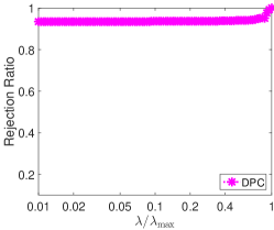
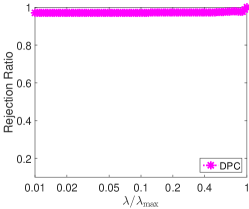
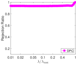
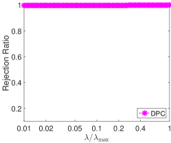
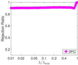
For Synthetic 1, the entries of each data matrix ${\bf X}_{t}$ are i.i.d. standard Gaussian with pairwise correlation zero, i.e., ${\rm corr}\left({\bf x}_{i}^{(t)},{\bf x}_{j}^{(t)}\right)=0$. For Synthetic 2, the entries of each data matrix ${\bf X}_{t}$ are drawn from i.i.d. standard Gaussian with pairwise correlation $0.5^{|i-j|}$, i.e., ${\rm corr}\left({\bf x}_{i}^{(t)},{\bf x}_{j}^{(t)}\right)=0.5^{|i-j|}$. To construct $\mathbf{w}_{t}^{*}$, we first randomly select $10\%$ of the features. Then, the corresponding components of $\mathbf{w}_{t}^{*}$ are populated from a standard Gaussian, and the remaining ones are set to $0$. For both Synthetic 1 and Synthetic 2, we set the feature dimension to $10000$, $20000$, and $50000$, respectively. For each setting, we run $20$ trials and report the average performance in Fig. 1 and Table 1.

(a) Synthetic 1, $d=10000$

(b) Synthetic 1, $d=20000$

(c) Synthetic 1, $d=50000$

(d) Synthetic 2, $d=10000$

(e) Synthetic 2, $d=20000$

(f) Synthetic 2, $d=50000$

Figure 1: Rejection ratios of DPC on two synthetic data sets with different feature dimensions.

Fig. 1 shows the rejection ratios of DPC on Synthetic 1 and Synthetic 2. For all the six settings, the rejection ratios of DPC are higher than $90\%$, even for small parameter values. This demonstrates one of the advantages of DPC, as previous empirical studies (El Ghaoui et al., 2012, Tibshirani et al., 2012, Wang et al., ) indicate that the capability of screening rules in identifying inactive features usually decreases as the parameter value decreases. Moreover, Fig. 1 also shows that as the feature dimension increases, the rejection ratios of DPC become higher—that is very close to $1$. This implies that the potential capability of DPC in identifying the inactive features on high-dimensional data sets would be even more significant.

Table 1 presents the running time of the solver with and without DPC. The speedup is very significant, which is up to $60$ times. Take Synthetic 1 for example. When the feature dimension is $50000$, the solver without DPC takes about $40.68$ hours to solve problem (1) at $100$ paramater values. In contrast, combined with DPC, the solver only takes less than one hour to solve the same $100$ problems—which leads to a speedup about $60$ times. Table 1 also shows that the computational cost of DPC is very low—which is negligible compared to that of the solver without screening. Moreover, as the rejection ratios of DPC increases with feature dimension growth (see Fig. 1), Table 1 shows that the speedup by DPC increases as well.

5.2 Experiments on Real Data Sets

We perform experiments on three real data sets: 1) the TDT2 text data set (Cai et al., 2009); 2) the animal data set (Lampert et al., 2009); 3) the Alzheimer’s Disease Neuroimaging Initiative (ADNI) data set (http://adni.loni.usc.edu/).

(a) Animal, $d=15036$

(b) TDT2, $d=24262$

(c) ADNI, $d=504095$

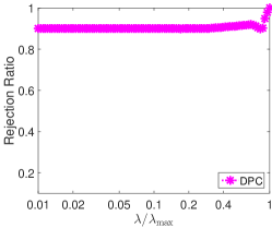
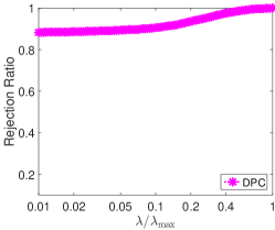
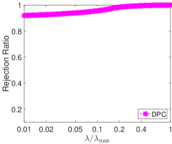
Figure 2: Rejection ratios of DPC on three real data sets.

The Animal Data Set The data set consists of $30475$ images of $50$ animals classes. By following the experiment settings in Kang et al. (2011), we choose $20$ animal classes in the data set: antelope, grizzly-bear, killer-whale, beaver, Dalmatian, Persiancat, horse, german- shepherd, blue-whale, Siamese-cat, skunk, ox, tiger, hippopotamus, leopard, moose, spidermonkey, humpback-whale, elephant, and gorilla. We construct $20$ tasks, where each of them is a classification task of one type of animal against all the others. For the $t^{th}$ task, we first randomly select $30$ samples from the $t^{th}$ class as the positive samples; and then we randomly select $30$ samples from all the other classes as the negative samples. We make use of all the seven sets of features kindly provided by Lampert et al. (2009): color histogram features, local self-similarity features, PyramidHOG (PHOG) features, SIFT features, colorSIFT features, SURF features, and DECAF features. Thus, each image is represented by a $15036$-dimensional vectors. Hence, the data matrix $X_{t}$ of the $t^{t}h$ task is of $60\times 15036$, where $t=1,\ldots,20$.

The TDT2 Data Set The original data set contains $9394$ documents of $30$ categories. Each document is represented by a $36771$-dimensional vector. Similar to the Animal data set, we construct $30$ tasks, each of which is a classification task of one category against all the others (Amit et al., 2007). Also, for the $t^{th}$ task, we first randomly select $50$ samples from the $t^{th}$ category as the positive samples, and then we randomly select $50$ samples from all the other categories as the negative samples. Moreover, we remove the features that have only zero entries, thus leaving us $24262$ features. Hence, the data matrix $X_{t}$ of the $t^{t}h$ task is of $100\times 24262$, where $t=1,\ldots,30$.

Table 1: Running time (in minutes) for solving the MTFL model (1) along a sequence of $100$ tuning parameter values of $\lambda$ equally spaced on the logarithmic scale of ${\lambda}/{\lambda_{\rm max}}$ from $1.0$ to $0.01$ by (a): the solver (Liu et al., 2009c) without screening (see the third column); (b): the solver with DPC (see the fifth column).

	$d$	solver	DPC	DPC+solver	speedup
Synthetic 1	$10000$	405.75	0.7	28.12	14.43
	$20000$	913.70	1.36	37.02	24.68
	$50000$	2441.57	3.50	42.08	58.03
Synthetic 2	$10000$	406.85	0.70	29.28	13.89
	$20000$	906.09	1.37	36.66	24.72
	$50000$	2435.38	3.46	44.78	54.39
Animal	15036	311.71	0.47	16.36	19.05
TDT2	24262	958.66	1.87	44.11	21.74
ADNI	504095	9625.58	21.13	35.34	272.37

The ADNI Data Set The data set consists of $747$ patients with $504095$ single nucleotide polymorphisms (SNPs), and the volume of $93$ brain regions for each patient. We first randomly select $20$ brain regions. Then, for each region, we randomly select $50$ patients, and utilize the corresponding SNPs data as the data matrix and the volumes of that brain region as the response. Thus, we have $20$ tasks, each of which is a regression task. The data matrix $X_{t}$ of the $t^{th}$ task is of $50\times 504095$, where $t=1,\ldots,20$.

Fig. 2 shows the rejection ratios of DPC—that are above $90\%$—on the aforementioned three real data sets. In particular, the rejection ratios of DPC on the ADNI data set are higher than $99\%$ at the $100$ parameter values. Table 1 shows that the resulting speedup is very significant—that is up to $270$ times. We note that the feature dimension of the ADNI data set is more than half million. Without screening, Table 1 shows that the solver takes about seven days (approximately one week) to compute the MTFL model (1) at $100$ parameter values. However, integrated with the DPC screening rule, the solver computes the $100$ solutions in about half an hour. The experiments again indicate that DPC provides better performance (in terms of rejection ratios and speedup) for higher dimensional data sets.

6 Conclusion

In this paper, we propose a novel screening method for the MTFL model in (1), called DPC. The DPC screening rule is based on an indepth analysis of the geometric properties of the dual problem and the dual feasible set. To the best of our knowledge, DPC is the first screening rule that is applicable to sparse models with multiple data matrices. DPC is safe in the sense that the identified features by DPC are guaranteed to have zero coefficients in the solution vectors across all tasks. Experiments on synthetic and real data sets demonstrate that DPC is very effective in identifying the inactive features, which leads to a substantial savings in computational cost and memory usage without sacrificing accuracy. Moreover, DPC is more effective as the feature dimension increases, which makes DPC a very competitive candidate for the applications of very high-dimensional data. We plan to extend DPC to more general MTFL models, e.g., the MTFL models with multiple regularizers.

Appendix A Discussions regarding to the Dual Problem of (1)

Although Eq. (9) implies that $\|\mathbf{m}^{\ell}\|\leq 1$, this might not be the case. Thus, we need to consider the following two cases.

1. If Eq. (9) holds, we can see that $\langle{\bf m}^{\ell},{\bf w}^{\ell}\rangle=\|{\bf w}^{\ell}\|$ and thus

   $$\min_{{\bf w}^{\ell}}\,f^{(\ell)}({\bf w}^{\ell})=0.$$ (31)

   Therefore, we have

   $$\min_{W}\,f(W)=0.$$ (32)

2. If Eq. (9) does not hold, i.e., $\|{\bf m}^{\ell}\|>1$, we would have

   $$\inf_{{\bf w}^{\ell}}\,f^{(\ell)}({\bf w}^{\ell})=-\infty,$$ (33)

   and thus

   $$\min_{W}\,f(W)=-\infty.$$ (34)

   To see this, we define ${\bf w}^{(\ell)}(t)=t\frac{{\bf m}^{\ell}}{\|{\bf m}^{\ell}\|}$ and thus

   $$\langle{\bf m}^{\ell},{\bf w}^{(\ell)}(t)\rangle=t\|{\bf m}^{\ell}\|.$$

   Then, we have

   $$f^{(\ell)}({\bf w}^{\ell}(t))=t(1-\|{\bf m}^{\ell}\|).$$ (35)

   Because $\|{\bf m}^{\ell}\|>1$, the above equation yields

   $$\inf_{{\bf w}^{\ell}}\,f^{(\ell)}({\bf w}^{\ell})\leq\lim_{t\rightarrow\infty}\,f_{2}^{(\ell)}({\bf w}^{\ell}(t))=-\infty.$$ (36)

The above discussion implies that

$$\min_{W}\,f(W)=\begin{dcases}0,\hskip 17.07164pt\mbox{if}\,\|{\bf m}^{\ell}\|\leq 1,\,\ell=1,\ldots,d,\\ -\infty,\hskip 5.69054pt\mbox{otherwise}.\end{dcases}$$ (37)

Appendix B Proof of Theorem 1

Proof.

For notational convenience, let

1. $\dfrac{\bf y}{\lambda}\in\mathcal{F}$;

2. $\theta^{*}(\lambda)=\dfrac{\bf y}{\lambda}$;

3. $W^{*}(\lambda)=0$;

4. $\lambda\geq\lambda_{\rm max}$.

Eq. (13) implies that 1 is equivalent to 2.

($2\Leftrightarrow 3$) Suppose that 2 holds. Eq. (14) implies that $X_{t}{\bf w}^{*}_{t}(\lambda)=0$ for $t=1,\ldots,T$. Denote the objective function of the MTFL model (1) by $f(W)$. We claim that $W^{*}(\lambda)$ must be zero. To see this, let $\overline{W}^{*}(\lambda)\neq 0$ be another optimal solution of (1) and thus $X_{t}\bar{\bf w}^{*}_{t}(\lambda)=0$ for $t=1,\ldots,T$. However, it is evident that $f(W^{*}(\lambda))<f(\overline{W}^{*}(\lambda))$. This leads to a contradiction. Thus, the optimal solution $W^{*}(\lambda)$ is zero and we have proved $2\Rightarrow 3$. The converse direction, i.e., $2\Leftarrow 3$ is a direct consequence of Eq. (14).

($1\Leftrightarrow 4$) It is evident that 1 holds if and only if ${\bf y}/\lambda$ is a feasible solution of problem (12), namely, all constraints in (12) holds at ${\bf y}/\lambda$. By plugging ${\bf y}/\lambda$ into the constraints in (12), we can see that the feasibility of ${\bf y}/\lambda$ is equivalent to 4. Thus, we can see that 1 is equivalent to 4. This completes the proof. ∎

Appendix C Proof of Corollary 4

Proof.

1. To show part 1, we only need to set ${\bf u}_{1}={\bf u}$ and ${\bf u}_{2}=0$, and then plug them into the inequality (3) [note that $\textup{P}_{\mathcal{C}}(0)=0$ since $0\in\mathcal{C}$].

2. Part 1 implies that $\|\textup{P}_{\mathcal{C}}({\bf u})\|\leq\|{\bf u}\|$. Thus, we have

   $$\|{\bf u}\|^{2}\geq\|{\bf u}\|\|\textup{P}_{\mathcal{C}}({\bf u})\|\geq\langle{\bf u},\textup{P}_{\mathcal{C}}({\bf u})\rangle,$$

   which is equivalent to the statement in part 2.

The proof is completed. ∎

Appendix D Proof of Theorem 5

We first cite some useful properties of the projection operators.

Lemma 10.

(Ruszczyński, 2006, Bauschke and Combettes, 2011) Let $\mathcal{C}$ be a nonempty closed convex set of a Hilbert space and $\mathbf{u}\in\mathcal{C}$. Then

1. $N_{\mathcal{C}}(\mathbf{u})=\{\mathbf{v}:\mathbf{P}_{\mathcal{C}}(\mathbf{u}+\mathbf{v})=\mathbf{u}\}$.

2. $\mathbf{P}_{\mathcal{C}}(\mathbf{u}+\mathbf{v})=\mathbf{u},\,\forall\,\mathbf{v}\in N_{\mathcal{C}}(\mathbf{u})$.

3. Let $\overline{\mathbf{u}}\notin\mathcal{C}$ and $\mathbf{u}=\mathbf{P}_{\mathcal{C}}(\overline{\mathbf{u}})$. Then, $\mathbf{P}_{\mathcal{C}}(\mathbf{u}+t(\overline{\mathbf{u}}-\mathbf{u}))=\mathbf{u}$ for all $t\geq 0$.

We are now ready to prove Theorem 5

Proof.

1. For $\lambda\in(0,\lambda_{\rm max})$, Theorem 1 implies that ${\bf y}/\lambda\notin\mathcal{F}$. Thus, the statement holds for $\lambda\in(0,\lambda_{\rm max})$ by Theorem 2 and Eq. (13) [let $\bar{\bf u}={\bf y}/\lambda$ and ${\bf u}=\theta^{*}(\lambda)$].

   To show the statement holds at $\lambda_{\rm max}$, Theorem 2 indicates that we need to show

   $$\left\langle\nabla g_{\ell_{*}}\left(\frac{\bf y}{\lambda_{\rm max}}\right),\theta-\frac{\bf y}{\lambda_{\rm max}}\right\rangle\leq 0,\,\forall\theta\in\mathcal{F}.$$ (38)

   Because $g_{\ell_{*}}(\cdot)$ is convex, we have (Ruszczyński, 2006)

   $$g_{\ell_{*}}(\theta)-g_{\ell_{*}}\left(\frac{{\bf y}}{\lambda_{\rm max}}\right)\geq\left\langle\nabla g_{\ell_{*}}\left(\frac{\bf y}{\lambda_{\rm max}}\right),\theta-\frac{\bf y}{\lambda_{\rm max}}\right\rangle.$$ (39)

   Note that, $g_{\ell}$ is the constraint function of the dual problem in (12). Thus, for any dual feasible solution $\theta\in\mathcal{F}$, it is evident that $g_{\ell_{*}}(\theta)\leq 1$. Moreover, Eq. (17) implies that $g_{\ell_{*}}({\bf y}/\lambda_{\rm max})=1$. Therefore, the left hand of the inequality (39) must be non-positive, which yields inequality (38). Thus, the statement holds.

2. A direct application of part 2 of Corollary 4 yields

   $$\left\langle\frac{\mathbf{y}}{\lambda_{0}},\mathbf{n}(\lambda_{0})\right\rangle=\left\langle\frac{\mathbf{y}}{\lambda_{0}},\frac{\mathbf{y}}{\lambda_{0}}-\theta^{*}(\lambda_{0})\right\rangle\geq 0,\,\forall\,\lambda_{0}\in(0,\lambda_{\rm max}).$$

   When $\lambda_{0}=\lambda_{\rm max}$, by noting that $\mathbf{n}(\lambda_{\rm max})=\nabla g_{\ell_{*}}(\tfrac{\mathbf{y}}{\lambda_{\rm max}})$, we have

   $$\left\langle\frac{\mathbf{y}}{\lambda_{\rm max}},\mathbf{n}(\lambda_{\rm max})\right\rangle=\sum_{t=1}^{T}2\left\langle\mathbf{x}_{\ell_{*}}^{(t)},\frac{\mathbf{y}}{\lambda_{\rm max}}\right\rangle^{2}\geq 0.$$

   Thus, the statement holds.

3. By Eq. (21), we have

   $$\langle\textbf{{r}}(\lambda,\lambda_{0}),\textbf{{n}}(\lambda_{0})\rangle=\left(\frac{1}{\lambda}-\frac{1}{\lambda_{0}}\right)\langle{\bf y},\textbf{{n}}(\lambda_{0})\rangle+\left\langle\frac{\bf y}{\lambda_{0}}-\theta^{*}(\lambda_{0}),\textbf{{n}}(\lambda_{0})\right\rangle.$$ (40)

   By Eqs. (20) and (13), the second term on the right hand side of Eq. (40) is nonnegative for all $\lambda_{0}\in(0,\lambda_{\rm max}]$.

   The fact that $0\in\mathcal{F}$ yields

   $$\left\langle 0-\frac{\bf y}{\lambda_{\rm max}},\textbf{{n}}(\lambda_{\rm max})\right\rangle\leq 0.$$

   Thus, the first term on the right hand side of Eq. (40) is nonnegative for $\lambda_{0}=\lambda_{\rm max}$. For $\lambda_{0}\in(0,\lambda_{\rm max})$, part 2 of Corollary 4, Eqs. (13) and (20) imply that

   $$\left\langle\frac{\bf y}{\lambda_{0}},\frac{\bf y}{\lambda_{0}}-\textup{P}_{\mathcal{F}}\left(\frac{\bf y}{\lambda_{0}}\right)\right\rangle=\left\langle\frac{\bf y}{\lambda_{0}},\textbf{{n}}(\lambda_{0})\right\rangle\geq 0.$$

   Thus, the first term on the right hand side of Eq. (40) is nonnegative for $\lambda_{0}\in(0,\lambda_{\rm max})$.

   As a result, the inner product $\langle\textbf{{r}}(\lambda,\lambda_{0}),\textbf{{n}}(\lambda_{0})\rangle$ is nonnegative.

4. We define

   $$\theta(t)=\theta^{*}(\lambda_{0})+t\textbf{{n}}(\lambda_{0}).$$ (41)

   Part 1 of Lemma 10 implies that

   $$\textup{P}_{\mathcal{F}}(\theta(t))=\theta^{*}(\lambda_{0}),\,\forall\,t\geq 0.$$ (42)

   The nonexpansiveness of the projection operators yields [let ${\bf u}_{1}={\bf y}/\lambda$ and ${\bf u}_{2}=\theta(t)$ and plug them into (3)]

   $$\left\|\textup{P}_{\mathcal{F}}\left(\frac{\bf y}{\lambda}\right)-\textup{P}_{\mathcal{F}}(\theta(t))\right\|^{2}+\|(\textup{P}_{\mathcal{F}}-\textup{Id})\left(\frac{\bf y}{\lambda}\right)-(\textup{P}_{\mathcal{F}}-\textup{Id})(\theta(t))\|^{2}\leq\left\|\frac{\bf y}{\lambda}-\theta(t)\right\|^{2},\,\forall\,t\geq 0.$$

   By Eqs. (13), (42) and (21), the above inequality reduces to

   $$\|\theta^{*}(\lambda)-\theta^{*}(\lambda_{0})\|^{2}+\|\theta^{*}(\lambda)-\theta^{*}(\lambda_{0})-(\textbf{{r}}(\lambda,\lambda_{0})-t\textbf{{n}}(\lambda_{0}))\|^{2}\leq\|\textbf{{r}}(\lambda,\lambda_{0})-t\textbf{{n}}(\lambda_{0})\|^{2},\,\forall\,t\geq 0.$$ (43)

   Let us consider

   $$\min_{t\geq 0}\,r(t)=\|\textbf{{r}}(\lambda,\lambda_{0})-t\textbf{{n}}(\lambda_{0})\|^{2}.$$ (44)

   Because $r(t)$ is a quadratic function of $t$, we can see that

   $$\min_{t\geq 0}\,r(t)=\begin{dcases}\|\textbf{{r}}(\lambda,\lambda_{0})\|^{2},\hskip 11.38109pt\mbox{if}\,\langle\textbf{{r}}(\lambda,\lambda_{0}),\textbf{{n}}(\lambda_{0})\rangle<0,\\ \|\textbf{{r}}^{\perp}(\lambda,\lambda_{0})\|^{2},\hskip 5.69054pt\mbox{if}\,\langle\textbf{{r}}(\lambda,\lambda_{0}),\textbf{{n}}(\lambda_{0})\rangle\geq 0.\end{dcases}$$

   Because of part 3, we have

   $$\min_{t\geq 0}\,r(t) =\|\textbf{{r}}^{\perp}(\lambda,\lambda_{0})\|^{2}$$ (45)

   $$\operatorname*{argmin}_{t\geq 0}\,r(t) =\frac{\langle\textbf{{r}}(\lambda,\lambda_{0}),\textbf{{n}}(\lambda_{0})\rangle}{\|\textbf{{n}}(\lambda_{0})\|^{2}}$$ (46)

   Plugging Eqs. (45) and (46) into (43) yields the statement, which completes the proof.

The proof is complete. ∎

References

• Amit et al. (2007) Y. Amit, M. Fink, N. Srebro, and S. Ullman. Uncovering shared structures in multiclass classification. In Proceedings of the 24th Annual International Conference on Machine Learning, 2007.
• Ando and Zhang (2005) R. Ando and T. Zhang. A framework for learning predictive structures from multiple tasks and unlabeled data. Journal of Machine Learning Research, 6:1817–1853, 2005.
• Argyriou et al. (2007) A. Argyriou, T. Evgeniou., and M. Pontil. Multi-task feature learning. In Advances in neural information processing systems, 2007.
• Argyriou et al. (2008) A. Argyriou, T. Evgeniou, and M. Pontil. Convex multi-task feature learning. Machine Learning, 73:243–272, 2008.
• Bakker and Heskes (2003) B. Bakker and T. Heskes. Task clustering and gating for bayesian multi ctask learning. Journal of Machine Learning Research, 4:83–99, 2003.
• Bauschke and Combettes (2011) H. H. Bauschke and P. L. Combettes. Convex Analysis and Monotone Operator Theory in Hilbert Spaces. Springer, 2011.
• Baxter (2000) J. Baxter. A model for inductive bias learning. Journal of Artificial Intelligence Research, 12:149–198, 2000.
• Ben-David and Schuller (2003) S. Ben-David and R. Schuller. Exploiting task relatedness for multiple task learning. In Proceedings of Computational Learning Theory, 2003.
• Cai et al. (2009) Deng Cai, Xuanhui Wang, and Xiaofei He. Probabilistic dyadic data analysis with local and global consistency. In Proceedings of the 26th Annual International Conference on Machine Learning, pages 105–112, 2009.
• Caruana (1997) R. Caruana. Multitask learning. Machine Learning, 28:41–75, 1997.
• Chen et al. (2013) J. Chen, L. Tang, J. Liu, and J. Ye. A convex formulation for learning shared structures from multiple tasks. IEEE Transactions on Pattern Analysis and Machine Intelligence, 35:1025–1038, 2013.
• El Ghaoui et al. (2012) L. El Ghaoui, V. Viallon, and T. Rabbani. Safe feature elimination in sparse supervised learning. Pacific Journal of Optimization, 8:667–698, 2012.
• Evgeniou et al. (2005) T. Evgeniou, C. Micchelli, and M. Pontil. Learning multiple tasks with kernel methods. Journal of Machine Learning Research, 6:615–637, 2005.
• Gay (1981) D. Gay. Computing optimal locally constrained steps. SIAM Journal on Scientific and Statistical Computing, 1981.
• Güler (2010) O. Güler. Foundations of Optimization. Springer, 2010.
• Kang et al. (2011) Z. Kang, K. Grauman, and F. Sha. Learning with whom to share in multi-task feature learning. In Proceedings of the 28th Annual International Conference on Machine Learning, 2011.
• Kim and Xing (2009) S. Kim and E. Xing. Tree-guided group lasso for multi-task regression with structured sparsity. In Proceedings of the 26th Annual International Conference on Machine Learning, 2009.
• Lampert et al. (2009) C. Lampert, H. Nickisch, and S. Harmeling. Learning to detect unseen object classes by between-class atttribute transfer. In IEEE Computer Society Conference on Computer Vision and Pattern Recognition, 2009.
• Liu et al. (2009a) H. Liu, M. Palatucci, and J. Zhang. Bsparsity coordinate descent procedures for the multi-task with applications to neural semantic basis discovery. In International Conference on Machine Learning, 2009a.
• Liu et al. (2009b) J. Liu, S. Ji, and J. Ye. Multi-task feature learning with efficient 2,1subscript21\ell_{2,1}-norm minimization. In The 25thsuperscript25𝑡25^{th} Conference on Uncertainty in Artificial Intelligence, 2009b.
• Liu et al. (2009c) J. Liu, S. Ji, and J. Ye. SLEP: Sparse Learning with Efficient Projections. Arizona State University, 2009c.
• Moré and Sorensen (1983) J. Moré and D. Sorensen. Computing a trust region step. SIAM Journal on Scientific and Statistical Computing, 1983.
• Ogawa et al. (2013) K. Ogawa, Y. Suzuki, and I. Takeuchi. Safe screening of non-support vectors in pathwise SVM computation. In Proceedings of the 30th Annual International Conference on Machine Learning, 2013.
• Ruszczyński (2006) A. Ruszczyński. Nonlinear Optimization. Princeton University Press, 2006.
• Sra (2012) S. Sra. Fast projections onto mixed-norm balls with applications. Data Mining and Knowledge Discovery, 2012.
• Tibshirani (1996) R. Tibshirani. Regression shringkage and selection via the lasso. Journal of the Royal Statistical Society Series B, 58:267–288, 1996.
• Tibshirani et al. (2012) R. Tibshirani, J. Bien, J. Friedman, T. Hastie, N. Simon, J. Taylor, and R. Tibshirani. Strong rules for discarding predictors in lasso-type problems. Journal of the Royal Statistical Society Series B, 74:245–266, 2012.
• Wang and Ye (2014) J. Wang and J. Ye. Two-layer feature reduction for sparse-group lasso via decomposition of convex sets. In Advances in Neural Information Processing Systems, 2014.
• (29) J. Wang, P. Wonka, and J. Ye. Lasso screening rules via dual polytope projection. Journal of Machine Learning Research, to appear.
• Wang et al. (2013a) J. Wang, J. Liu, and J. Ye. Efficient mixed-norm regularization: Algorithms and safe screening methods. arXiv:1307.4156, 2013a.
• Wang et al. (2013b) J. Wang, J. Zhou, P. Wonka, and J. Ye. Lasso screening rules via dual polytope projection. In Advances in Neural Information Processing Systems, 2013b.
• Wang et al. (2014a) J. Wang, P. Wonka, and J. Ye. Scaling SVM and least absolute deviations via exact data reduction. In Proceedings of the 31th Annual International Conference on Machine Learning, 2014a.
• Wang et al. (2014b) J. Wang, J. Zhou, J. Liu, P. Wonka, and J. Ye. A safe screening rule for sparse logistic regression. In Advances in Neural Information Processing Systems, 2014b.
• Xiang et al. (2011) Z. J. Xiang, H. Xu, and P. J. Ramadge. Learning sparse representation of high dimensional data on large scale dictionaries. In Advances in Neural Information Processing Systems, 2011.
• Zhang et al. (2006) J. Zhang, Z. Ghahramani, and Y. Yang. Learning multiple related tasks using latent independent component analysis. In Advances in Neural Information Processing Systems, 2006.
• Zhang et al. (2010) Y. Zhang, D. Yeung, and Q. Xu. Probabilistic multi-task feature selection. In Advances in Neural Information Processing Systems, 2010.
• Zhou et al. (2012) J. Zhou, J. Liu, V. Narayan, and J. Ye. Modeling disease progression via fused sparse group lasso. In International Conference On Knowledge Discovery and Data Mining, 2012.
• Zou and Hastie (2005) H. Zou and T. Hastie. Regularization and variable selection via the elastic net. Journal of the Royal Statistical Society Series B, 67:301–320, 2005.