Frequency shifts of resonant modes of the Sun due to near-surface convective scattering

Abstract

Measurements of oscillation frequencies of the Sun and stars can provide important independent constraints on their internal structure and dynamics. Seismic models of these oscillations are used to connect structure and rotation of the star to its resonant frequencies, which are then compared with observations, the goal being that of minimizing the difference between the two. Even in the case of the Sun, for which structure models are highly tuned, observed frequencies show systematic deviations from modeled frequencies, a phenomenon referred to as the “surface term”. The dominant source of this systematic effect is thought to be vigorous near-surface convection, which is not well accounted for in both stellar modeling and mode-oscillation physics. Here we bring to bear the method of homogenization, applicable in the asymptotic limit of large wavelengths (in comparison to the correlation scale of convection), to characterize the effect of small-scale surface convection on resonant-mode frequencies in the Sun. We show that the full oscillation equations, in the presence of temporally stationary 3-D flows, can be reduced to an effective “quiet-Sun” wave equation with altered sound speed, Brünt–Väisäla frequency and Lamb frequency. We derive the modified equation and relations for the appropriate averaging of three dimensional flows and thermal quantities to obtain the properties of this effective medium. Using flows obtained from three dimensional numerical simulations of near-surface convection, we quantify their effect on solar oscillation frequencies, and find that they are shifted systematically and substantially. We argue therefore that consistent interpretations of resonant frequencies must include modifications to the wave equation that effectively capture the impact of vigorous hydrodynamic convection.

1. Introduction

Measurements of oscillation frequencies of stars provide some of the strongest constraints on stellar structure models. Recent missions Kepler (Borucki et al., 2010) and COROT (Auvergne et al., 2009) have provided us with high quality asteroseismic data, which have revealed structural features of Sun-like stars in unprecedented detail. There have been several successful solar models which have reproduced the oscillation frequencies to within a few parts in thousand. Despite this degree of accuracy, the modeled frequencies display systematic deviations from the observed ones. Understanding the root of these deviations is important both from theoretical and observational point of view — not only is it a window into the missing physics, it is also a hindrance in fitting stellar models. With the ever increasing precision in measured frequencies, it is imperative to understand the physical reason behind the trend and to correct for it while extracting information about the Sun at the same time.

There are various reasons why these shifts are observed, which were categorized as model and modal effects by (Rosenthal et al., 1999) . Some of the possible sources for this bias are:

1. Errors in physics that go into the modeling, including turbulent-pressure contributions (model effect).

2. Non-adiabaticity prevalent in the outer layers of the Sun (model+modal effect).

3. Imprecise modeling of propagation of waves through convective flows near the surface of the Sun (modal effect).

4. Non-linearity in the wave equation (modal effect).

It is unlikely that any one of these mechanisms would explain the observed deviations completely, rather a combination of these corrections would lead to a better estimate of oscillation frequencies, and possibly eliminate the observed bias. We would like to differentiate between the first and third points — the first assumes a hydrodynamic equilibrium model, but treats oscillations as if they were about an equivalent hydrostatic background, while the third treats the oscillations about a dynamic background. In this article we focus on the third aspect, and propose a method to correct the modal effect. Strong convective flows with speeds close to the sound speed exist near the surface of the Sun. We show that advection of traveling waves by these flows can have a significant impact on the resonant mode frequencies, and it is therefore important to account for this effect in order to extract the correct physics from measurements.

Acoustic modes (p modes) are standing waves bounded from below by a lower turning point set by the Lamb frequency, and from above by an upper turning point set by the acoustic-cutoff frequency. The upper turning point for modes with frequencies below $2\,\mathrm{mHz}$ is significantly below the surface of the Sun, but modes with frequencies lying in the range $2\,\mathrm{mHz}$ to $5\,\mathrm{mHz}$ encounter an upper turning point close to the surface. These are the modes for which the measured frequencies display a systematic deviation from model, hence it seems likely that the missing physics lies close to the surface, and the deviation is often termed ‘surface effect’. The deviation is predominantly a function of the frequency of a mode, hence corrective terms should also be functions of the mode frequency. An early attempt at mitigating the frequency differences was by Gough (1990), whose prescription was in the form of a power law correction based on the physical process involved: fibrillated magnetic fields lead to a change in sound speed, and hence an observed frequency $\nu$ would be shifted by $\delta\nu\propto\nu^{3}/\mathcal{I}$, where $\mathcal{I}$ is the mode inertia; while alternate parametrizations of convection lead to a shift $\delta\nu\propto 1/\left(\nu\mathcal{I}\right)$. Kjeldsen et al. (2008) had studied the shifts in the Sun, and with an empirical power law model $\delta\nu=a\left(\nu/\nu_{0}\right)^{b}$, were able to correct for the shifts in $\alpha\;\mathrm{Cen}\;\mathrm{A}$, $\alpha\;\mathrm{Cen}\;\mathrm{B}$ and $\beta\;\mathrm{Hyi}$. Recently Ball & Gizon (2014) have shown that a combination of the two effects studied by Gough — the cubic shift and the inverse shift — is able to fit the deviations better than Kjeldsen’s power law. These corrections are satisfactory from a model-fitting viewpoint, but by eliminating the frequency differences altogether we lose information about their origin.

Despite the high flow speeds, there still exists a small parameter in the wave equation — the granulation length scales are usually much smaller than horizontal wavelengths of low-$\ell$ modes, which are of the order of the solar radius. Hanasoge et al. (2013) had designed an alternate approach to deal with small-scale sound speed perturbation, by expanding the wave equation in terms of the ratio of the two length scales, followed by averaging over small scales. They had shown that if the horizontal wavelength of a propagating wave is much larger than the length scale over which the background medium fluctuates, it is possible to replace the background by a homogeneous, coarse-grained one. In this paper, we use a similar analysis in presence of small-scale flows, and derive an expression for an effective speed. A way to think of homogenization is as follows: near-surface convection is a stochastic process, evolving both temporally and spatially. Here we assume temporally stationarity, with waves propagating through a frozen configuration of convective flows. Precise measurements of resonant frequencies require taking spectra of long sequences of raw observations of the wavefield — at a minimum, several oscillation periods but typically much longer than that, on the order of a million periods, so as to resolve the mode line-width and beat down the noise sufficiently. Over this time, waves will have propagated through a large number of realizations of convective flows. Thus one may think of this as an ensemble of wave equations, each ascribed a set of coefficients corresponding to different realizations of the process of convection, drawn from the same probability density function. Each realization of convective flows corresponds to a wave solution, and the question then becomes: how to obtain an ensemble average of these wave solutions? Homogenization provides an answer to this question, specifically in the limit where the horizontal wavelength is much larger than the length scale corresponding to the flows. The principle behind homogenization is that in cases where waves and flows are scale-separated, measurables such as frequencies can be reproduced by studying wave-propagation through a quiet, homogeneous medium obtained by appropriately averaging over small-scale flows. The method has an advantage that the effective speed which governs wave behaviour on a large-scale emerges naturally out of the averaging process. In the asymptotic limit, this is the speed which shall appear in the dispersion relation, and hence shall determine the observed frequency differences. The method of homogenization allows an extension to random media where the distribution function is translationally invariant and bounded (Papanicolaou & Varadhan, 1982), and thus holds promise in progressing beyond our simplified analysis to real solar models.

Several authors such as Murawski & Roberts (1993); Duvall et al. (1998) had studied the effect of random scatterings by convective flows on surface gravity waves (f modes), arriving at corrections to the dispersion relation in order to match the observed frequencies and line-widths. A different treatment to capture the effect of flows on p modes had been carried out by Brown (1984), who had proposed a correction of the form $\left(1-\langle v_{z}^{2}\rangle/c^{2}\right)$ by carrying out a horizontal average over the wave equation. This form of the correction comes closest to our approach, which generalizes the analysis to arbitrary small-scale vector flow velocities. An asymptotic analysis of p-mode frequency shifts for small Mach numbers had been carried out by Stix & Zhugzhda (2004), but whether the analysis extends to transonic flows near the solar surface remains unclear.

2. Governing Dynamics

Waves on the Sun are modeled as small-amplitude perturbations about a background, which we assume to be in a steady state. The background medium is characterized by its pressure $p\left(\mathbf{x}\right)$, density $\rho\left(\mathbf{x}\right)$, flow velocity ${\bf u}\left(\mathbf{x}\right)$, and gravitational potential $\phi\left(\mathbf{x}\right)$. Waves shall induce oscillations about the temporarily stationary background, and the velocity of a moving blob would be given by a sum of the background flow velocity and the mode velocity. We work with the vector flow velocity $\mathbf{u}\left(\mathbf{x}\right)$ without splitting it up into horizontal and vertical components, since both the components repeat over small scales horizontally and hence can be treated analogously. In further analysis, we shall suppress explicit spatial and temporal dependence for notational convenience. The full magnetohydrodynamic equation for waves traveling through non-uniform flows was analyzed by Webb et al. (2005), we replicate the equation of motion here. The background flow field $\mathbf{u}$ satisfies the equation

$$\bm{\nabla}\cdot\left(\rho{\bf uu}+p\mathbf{I}\right)+\rho\bm{\nabla}\phi=\bm{0},$$ (1)

where $\mathbf{I}$ denotes the second-rank identity tensor defined as $\mathbf{I}_{ij}=\delta_{ij}$. In presence of a flow field ${\bf u}$, the material derivative of a small-amplitude displacement $\bm{\xi}\left(\mathbf{x},t\right)$ is defined as

$$\dot{\bm{\xi}}=\partial_{t}\bm{\xi}+{\bf u}\cdot\bm{\nabla}\bm{\xi}.$$ (2)

We assume that there exists a flow field which satisfies the background equations, and concentrate on the wave equation. The acoustic wave equation, to linear order in the perturbations, is given by

$$\partial_{t}\left(\rho\dot{\bm{\xi}}\right)+\bm{\nabla}\cdot\Big{\{}\rho{\bf u}\dot{\bm{\xi}}+\mathbf{I}\left(p-\rho c^{2}\right)\bm{\nabla}\cdot\bm{\xi}-p\left(\bm{\nabla}\bm{\xi}\right)^{T}\Big{\}}$$

$$+\rho\bm{\xi}\cdot\bm{\nabla}\bm{\nabla}\phi=\bm{0},$$ (3)

where $T$ in the exponent denotes the transpose operator (Webb et al., 2005). We shall stick to the Cowling approximation as our focus is on correcting for the wave speed; the analysis can be extended to a general case in an analogous manner.

A propagating wave is scattered out in all direction by the background flow field, which results in a change in the phase of the forward-traveling wave. Multiple scattering would lead to repeated phase shifts, leading to an altered phase velocity of the wave. This modified velocity would govern the dispersion relation, which would in turn determine the oscillation frequencies. In order to model this scattering perturbatively, we resort to the multiple scale approach of spatial homogenization.

3. Spatial Homogenization

Low-degree resonant modes on the sun have horizontal wavelengths ($\lambda$) comparable to the solar radius, which is much larger than the typical length scales of granulation on the Sun ($L$). In such a case, the dynamics can be parametrized in terms of the scale ratio $\varepsilon=L/\lambda$. In the limit $\varepsilon\ll 1$, we can replace the rapidly fluctuating medium by a homogeneous, albeit anisotropic one. To illustrate this approach, we study a special case of a periodic flow in a Cartesian box, where we denote the vertical depth by the coordinate $z$, and label a point on a horizontal plane by the coordinates $\left(x,y\right)$. The background medium repeats after a length $L$ along both the horizontal directions $x$ and $y$, and is stratified in the vertical direction. On a particular horizontal plane, the flow takes the form of tessellated square cells. To study the dynamics in the asymptotic limit $\varepsilon\ll 1$, we introduce two spatial coordinates which are scale-separated: a slow coordinate $\mathbf{x}=\left(x,y,z\right)$ and a horizontal fast coordinate $\mathbf{x}_{h}^{\prime}=\left(x/\varepsilon,y/\varepsilon\right)$. Note that the vertical component of mode wavelength can be comparable to the scale of flows, so the advection terms might not be scale-separable vertically. Bearing this in mind, scale separation is being carried out strictly in the horizontal directions, labeled by $x-y$ or equivalently by $\mathbf{x}_{h}^{\prime}$. The depth coordinate $z$ is common to the flows and the wave, and it characterizes the dynamics completely in the vertical direction. In terms of these new coordinates, the spatial gradient can be rewritten as

$$\bm{\nabla}=\bm{\nabla}_{\mathbf{x}}+1/\varepsilon\bm{\nabla}_{\mathbf{h}},$$ (4)

where $\bm{\nabla}_{\mathbf{x}}$ acts over the coordinates denoted by $\mathbf{x}$, and $\bm{\nabla}_{\mathbf{h}}$ acts over the fast horizontal coordinates denoted by $\mathbf{x}_{h}^{\prime}$.

We expand the wave field $\bm{\xi}$ as a perturbative series in the small parameter $\varepsilon$ as

$$\bm{\xi}\left(\mathbf{x},\mathbf{x}_{h}^{\prime},t\right) = \bm{\xi_{0}}\left(\mathbf{x},\mathbf{x}_{h}^{\prime},t\right)+\varepsilon\bm{\xi_{1}}\left(\mathbf{x},\mathbf{x}_{h}^{\prime},t\right)$$ (5)

$$+\varepsilon^{2}\bm{\xi_{2}}\left(\mathbf{x},\mathbf{x}_{h}^{\prime},t\right)+\mathcal{O}\left(\varepsilon^{3}\right).$$

The term at order $\varepsilon^{0}$ represents the large-scale characteristics of the wave field, while the higher-order terms arise as the incoming wave is scattered by the flows. This approach differs from standard perturbative expansions in two ways — firstly the expansion parameter is not in terms of the flow speed $u$ but the length scale $L$; secondly the zeroth-order field is not a solution to an equation without flows, but senses an average effect of the flows. Our approach would be to replace the spatially varying medium by an equivalent quiet background, which is different from what would have been there had there been no flows. We substitute Equation (5) in Equation (3) and use Equation (2) to write down the equations order by order in $\varepsilon$.

At order $\varepsilon^{-2}$ we get

$$\mathcal{L}^{\left(-2\right)}\bm{\xi_{0}}+\rho\bm{\xi_{0}}\cdot\bm{\nabla}_{\mathbf{h}}\bm{\nabla}_{\mathbf{h}}\phi=\bm{0},$$ (6)

where

$$\mathcal{L}^{\left(-2\right)}\bm{\xi}=\bm{\nabla}_{\mathbf{h}}\cdot\Big{\{}\rho{\bf uu}\cdot\bm{\nabla}_{\mathbf{h}}\bm{\xi}+\mathbf{I}\left(p-\rho c^{2}\right)\bm{\nabla}_{\mathbf{h}}\cdot\bm{\xi}-p\left(\bm{\nabla}_{\mathbf{h}}\bm{\xi}\right)^{T}\Big{\}}.$$ (7)

We introduce an alternate definition of the operator $\mathcal{L}^{\left(-2\right)}$ by defining the transpose map explicitly. We introduce the following tensors and tensorial relations:

• The double-dot product of two dyadic tensors $\mathbf{A}$ and $\mathbf{B}$ defined as $\mathbf{A}:\mathbf{B}=A_{ij}B_{ij}$, where repeated indices are summed over. This definition can be extended to higher order tensors $\tilde{\mathbf{A}}$ and $\tilde{\mathbf{B}}$, where the last two indices of $\tilde{\mathbf{A}}$ and the first two of $\tilde{\mathbf{B}}$ shall be contracted.

• A fourth order tensor $\tilde{\mathbf{T}}$ defined as $\tilde{\mathbf{T}}_{ijkl}=\delta_{il}\delta_{jk}$. The tensor $\tilde{\mathbf{T}}$ has the property $\tilde{\mathbf{T}}:\mathbf{D}=\mathbf{D}^{T}$ for a dyadic tensor $\mathbf{D}$. The definition can be extended to higher-order tensors, where the transpose operator $\tilde{\mathbf{T}}$ flips the first two indices.

• A fourth-rank tensor $\tilde{\mathbf{I}}_{4}$, defined as $\tilde{\mathbf{I}}_{4}{}_{ijkl}=\delta_{ik}\delta_{jl}$, that satisfies $\tilde{\mathbf{I}}_{4}:\mathbf{D}=\mathbf{D}$ for any dyadic tensor $\mathbf{D}$.

We define the tensor

$$\tilde{\bm{\Gamma}}=\rho{\bf uu}\cdot\tilde{\mathbf{I}}_{4}+\mathbf{I}\left(p-\rho c^{2}\right)\mathbf{I}-p\tilde{\mathbf{T}}$$ (8)

in terms of which we can rewrite the operator $\mathcal{L}^{\left(-2\right)}$ as

$$\mathcal{L}^{\left(-2\right)}\bm{\xi}=\bm{\nabla}_{\mathbf{h}}\cdot\left(\tilde{\bm{\Gamma}}:\bm{\nabla}_{\mathbf{h}}\,\bm{\xi}\right).$$ (9)

We shall assume henceforth that the gravitational potential $\phi$ is independent of the fast coordinate $\mathbf{x}_{h}^{\prime}$, which lets us drop any term like $\bm{\nabla}_{\mathbf{h}}\phi$ or $\bm{\nabla}_{\mathbf{h}}\bm{\nabla}_{\mathbf{x}}\phi$. This assumption is reasonably justified, since density in the near-surface layers is much smaller than the interior and hence the gravitational potential would depend only weakly on the flows near the surface. Under this assumption, Eq. (6) becomes

$$\mathcal{L}^{\left(-2\right)}\bm{\xi_{0}}=\bm{0}.$$ (10)

A particular solution to Equation (10) is a zeroth-order field $\bm{\xi_{0}}$ that is independent of the fast coordinate $\mathbf{x}_{h}^{\prime}$. This is a sufficient, but not a necessary condition. A general solution to Equation (10) can be a function of $\mathbf{x}_{h}^{\prime}$, which means the operator $\mathcal{L}^{\left(-2\right)}$ might be singular. We shall need to invert this operator at order $\varepsilon^{-1}$, so it might be necessary to define the inverse precisely by imposing boundary conditions on the fields, or as a generalized inverse, which is beyond the scope of this paper. We shall proceed assuming that $\bm{\xi_{0}}$ is independent of $\mathbf{x}_{h}^{\prime}$, which fits into our picture of perturbations about a homogeneous background.

Collecting terms of the order $\varepsilon^{-1}$, we obtain

$$\mathcal{L}^{\left(-2\right)}\bm{\xi_{1}}+\mathcal{L}^{\left(-1\right)}\bm{\xi_{0}}=\bm{0},$$ (11)

where

$$\mathcal{L}^{\left(-1\right)}\bm{\xi}=\bm{\nabla}_{\mathbf{h}}\cdot\left(\tilde{\bm{\Gamma}}:\bm{\nabla}_{\mathbf{x}}\,\bm{\xi}\right),$$ (12)

and $\mathcal{L}^{\left(-2\right)}$ is as defined in Equation (9). We use the fact that $\bm{\xi_{0}}$ is independent of $\mathbf{x}_{h}^{\prime}$ to rewrite Equation (11) as

$$\bm{\nabla}_{\mathbf{h}}\cdot\left(\tilde{\bm{\Gamma}}:\bm{\nabla}_{\mathbf{h}}\bm{\xi_{1}}\right)=-\left(\bm{\nabla}_{\mathbf{h}}\cdot\tilde{\bm{\Gamma}}\right):\bm{\nabla}_{\mathbf{x}}\,\bm{\xi_{0}}$$ (13)

We note two facts - firstly, Equation (13) is linear in $\bm{\xi_{1}}$, secondly, the right hand side is a product of two terms, one of which varies horizontally over the slow scale $\mathbf{x}$ while the other varies over the fast scale $\mathbf{x}_{h}^{\prime}$. This motivates us to seek solutions for $\bm{\xi_{1}}$ by separating the slowly varying horizontal components of $\mathbf{x}$ from the rapidly varying components of $\mathbf{x}_{h}^{\prime}$. We substitute

$$\bm{\xi_{1}}=\tilde{\mathbf{J}}\left(\mathbf{x}_{h}^{\prime},z\right):\bm{\nabla}_{\mathbf{x}}\,\bm{\xi_{0}}$$ (14)

where $\tilde{\mathbf{J}}\left(\mathbf{x}_{h}^{\prime},z\right)$ is a third-rank tensor. Substituting Equation (14) in Equation (11), and using the fact that $\bm{\xi_{0}}$ is independent of $\mathbf{x}_{h}^{\prime}$, we obtain

$$\left[\mathcal{L}^{\left(-2\right)}\tilde{\mathbf{J}}+\bm{\nabla}_{\mathbf{h}}\cdot\tilde{\bm{\Gamma}}\right]:\bm{\nabla}_{\mathbf{x}}\,\bm{\xi_{0}} = \bm{0}.$$ (15)

We seek a solution $\tilde{\mathbf{J}}$ which satisfies

$$\mathcal{L}^{\left(-2\right)}\tilde{\mathbf{J}}=-\bm{\nabla}_{\mathbf{h}}\cdot\tilde{\bm{\Gamma}}.$$ (16)

This is conventionally known as a cell problem (see e.g. Bensoussan et al., 1978).

At order $\varepsilon^{0}$ we get the equation of motion for the zeroth-order field $\bm{\xi_{0}}$

$$\rho\,\partial_{t}\bm{\xi_{0}}+\rho{\bf u}\cdot\partial_{t}\left(\bm{\nabla}_{\mathbf{x}}\,\bm{\xi_{0}}+\bm{\nabla}_{\mathbf{h}}\,\bm{\xi_{1}}\right)$$

$$+\mathcal{L}^{\left(0\right)}\bm{\xi_{0}}+\mathcal{L}^{\left(1\right)}\bm{\xi_{1}}+\mathcal{L}^{\left(-1\right)}\bm{\xi_{1}}+\mathcal{L}^{\left(-2\right)}\bm{\xi_{2}}$$

$$+\rho\,\bm{\xi_{0}}\cdot\bm{\nabla}_{\mathbf{x}}\bm{\nabla}_{\mathbf{x}}\phi = \bm{0},$$ (17)

where

$$\mathcal{L}^{\left(0\right)}\bm{\xi} = \bm{\nabla}_{\mathbf{x}}\cdot\left\{\tilde{\bm{\Gamma}}:\bm{\nabla}_{\mathbf{x}}\,\bm{\xi}\right\},$$ (18)

$$\mathcal{L}^{\left(1\right)}\bm{\xi} = \bm{\nabla}_{\mathbf{x}}\cdot\left\{\tilde{\bm{\Gamma}}:\bm{\nabla}_{\mathbf{h}}\,\bm{\xi}\right\}.$$ (19)

We know that the first order field $\bm{\xi_{1}}$ depends on the zeroth-order field $\bm{\xi_{0}}$ through Equation (14); we substitute this in Equation (17) and average over the fast coordinate $\mathbf{x}_{h}^{\prime}$. The averaging process restricts us to the zero-spatial-frequency mode, however we do retain information about smaller length scales through $\tilde{\mathbf{J}}$. Given a horizontal cell $\mathcal{B}=[0,L)\times[0,L)$, we define the cell average of a function $f\left(\mathbf{x}_{h}^{\prime}\right)$ as

$$\left\langle f\right\rangle=\frac{1}{L^{2}}\int_{\mathcal{B}}d\mathbf{x}_{h}^{\prime}\,f\left(\mathbf{x}_{h}^{\prime}\right).$$ (20)

The terms $\mathcal{L}^{\left(-1\right)}\bm{\xi_{1}}$ and $\mathcal{L}^{\left(-2\right)}\bm{\xi_{2}}$ in Equation (17) are total divergences in $\mathbf{x}_{h}^{\prime}$, so they drop off on averaging as we impose periodic boundary conditions. We obtain

$$\langle\rho\rangle\partial_{t}^{2}\bm{\xi_{0}}+2\langle\rho{\bf u}\rangle\cdot\bm{\nabla}_{\mathbf{x}}\,\partial_{t}\,\bm{\xi_{0}}$$

$$-\bm{\nabla}_{\mathbf{x}}\cdot\left[\langle\rho\tilde{\mathbf{C}}\rangle:\bm{\nabla}_{\mathbf{x}}\bm{\xi_{0}}\right]+\bm{\xi_{0}}\cdot\langle\rho\bm{\nabla}_{\mathbf{x}}\bm{\nabla}_{\mathbf{x}}\phi\rangle = 0,$$ (21)

where

$$\tilde{\mathbf{C}}=\tilde{\bm{\Gamma}}:\left(\tilde{\mathbf{I}}_{4}+\bm{\nabla}_{\mathbf{h}}\tilde{\mathbf{J}}\right)$$ (22)

resembles a wave speed squared term that governs wave propagation on large scales. This is similar in form to the result obtained by Brown (1984), except the term $\tilde{\mathbf{J}}$ which arises from the separation of scales. We can substitute for $\tilde{\bm{\Gamma}}$ from Equation (8) to recast Equation (22) in a more tangible form as

$$\tilde{\mathbf{C}} = \left(c^{2}-\frac{p}{\rho}\right)\mathbf{I}\,\mathbf{I}-{\bf uu}\cdot\tilde{\mathbf{I}}_{4}+\frac{p}{\rho}\tilde{\mathbf{T}}$$ (23)

$$+ \mathrm{terms\;arising\;from\;cell\;problem}.$$

Convective cells on the surface of the Sun have a structural form where hot gas rises up near the center and cooler gas sinks down around the edges of the cell. We assume that the flow in a particular cell is anti-symmetric about the cell center, hence $\langle\rho\mathbf{u}\rangle=\bm{0}$. This lets us drop the advective term in Equation (21) and obtain

$$\langle\rho\rangle\partial_{t}^{2}\bm{\xi_{0}}-\bm{\nabla}_{\mathbf{x}}\cdot\left[\langle\rho\tilde{\mathbf{C}}\rangle:\bm{\nabla}_{\mathbf{x}}\,\bm{\xi_{0}}\right]+\bm{\xi_{0}}\cdot\langle\rho\bm{\nabla}_{\mathbf{x}}\bm{\nabla}_{\mathbf{x}}\phi\rangle=\bm{0}.$$ (24)

Equation (24) is the homogenized wave equation, wherein we have replaced the spatially fluctuating background medium by an effective homogeneous, anisotropic one. The effective speed depends on both the horizontal and vertical flow profiles, the sound speed profile and the density. If density variations in a cell are spatially correlated with the flow speeds, a description in terms of the average speeds and average densities which ignores correlations might not be sufficient.

Periodicity of flows along specific directions leads to a tensorial wave speed, hence we expect anisotropy in wave propagation. Equation (24) is a standard eigenvalue problem which we can solve to find the dispersion relation $\omega\left(n,{\bf k}\right)$ for vertical order $n$ and horizontal wave vector ${\bf k}$. This dispersion relation captures the extent to which the frequency of a monochromatic wave would appear to differ from the canonical dispersion relation $\omega=ck$, which is governed only by the adiabatic sound speed. As an example, we consider waves propagating in a 2-dimensional uniformly dense fluid. We assume that the fluid film is tiled with small-scale, periodic flows $\mathbf{u}=\left(u_{x},u_{y}\right)$. A plane wave propagating along the $x$ axis would have the form

$$\bm{\xi_{0}}\left(\mathbf{x}\right)=\mathbf{A}\exp\left(\mathrm{i}\left(k_{x}x-\omega t\right)\right),$$ (25)

where $\mathbf{A}=\left(A_{x},A_{y}\right)$ is the amplitude, $k_{x}$ is the $x$ component of the wave-vector and $\omega$ is the frequency of the wave. Neglecting changes in gravitational field $\bm{\nabla}_{\mathbf{x}}\phi$ in the plane, we can rewrite Equation (24) in Fourier space as

$$\omega^{2}\left(\begin{array}[]{c}A_{x}\\ A_{y}\end{array}\right)=k_{x}^{2}\left(\begin{array}[]{cc}\langle c^{2}-u_{x}^{2}+\mathrm{c.p_{1}}\rangle&\langle\mathrm{c.p_{2}}\rangle\\ \langle\mathrm{c.p_{3}}\rangle&\langle-u_{x}^{2}+\mathrm{c.p_{4}}\rangle\end{array}\right)\left(\begin{array}[]{c}A_{x}\\ A_{y}\end{array}\right),$$ (26)

where the terms referred to as $\mathrm{c.p}_{1}$ to $\mathrm{c.p}_{4}$ arise from the solution to the cell problem. The corresponding dispersion relation can be obtained by diagonalizing the matrix in the second term of Equation (26). If the terms $\mathrm{c.p}_{1}$ to $\mathrm{c.p}_{4}$ are negligible, the dispersion relation would have the form $\omega=\langle\sqrt{c^{2}-u_{x}^{2}}\rangle k_{x}$, but this might not be a good approximation in general.

We note that Equation (24) is not damped at the leading order, so attenuation, if any, would be captured at a higher order. This is consistent with observations, since the observed p-mode line-widths are much smaller than the corresponding frequencies.

4. Numerical test of flow homogenization

In this section we take a simple example of waves propagating through flows in a 2-D plane, and show that we can effectively reproduce the wave speed by homogenizing over small scale flows. A thorough analysis of the approach would include realistic pressure, density and sound-speed profiles, possibly starting from simulations of near-surface structure of stars. In this work, we focus only on sound-speed variations induced by flows, and assume that the background pressure and gravitational field are unchanged in presence of the flow. We also assume that the background medium is uniformly dense throughout. Under these assumptions, Equation (3) simplifies considerably as we can drop the terms $\bm{\nabla}\cdot\left(\mathbf{I}p\bm{\nabla}\cdot\bm{\xi}-p\left(\bm{\nabla}\bm{\xi}\right)^{T}\right)$ and $\bm{\xi}\cdot\bm{\nabla}\bm{\nabla}\phi$. We combine Equations (2) and (3) to obtain

$$\partial_{t}^{2}\bm{\xi}+2{\bf u}\cdot\bm{\nabla}\partial_{t}\bm{\xi}+\left({\bf u}\cdot\bm{\nabla}\right)^{2}\bm{\xi}-\bm{\nabla}\left(c^{2}\bm{\nabla}\cdot\bm{\xi}\right)=\bm{0}.$$ (27)

We assume that the waves are propagating in a medium that is periodic along both the directions; in other words, the unit box $\mathcal{B}=[0,L)\times[0,L)$ is tessellated to fill up the entire two-dimensional plane. We choose to work in Cartesian coordinates $\left(x,y\right)$, with the origin at the center of a cell. As an example of a flow-field in a cell, we choose a vortex centered about the cell-center. The functional form of the flow is given by

$${\bf u}=u_{0}\frac{\left(x\hat{y}-y\hat{x}\right)}{\sigma}\exp\left(-\frac{\left(x^{2}+y^{2}\right)}{2\sigma^{2}}\right),$$ (28)

where $u_{0}$ is a velocity scale, $\sigma$ is a length scale of the flow related to the cell-size $L$. The sound speed $c$ would depend on several factors such as the pressure in a cell and the equation of state. For our illustrative purpose, we choose a simple model given by

$$c\left(r\right)^{2}=c_{\infty}^{2}+\left(c_{0}^{2}-c_{\infty}^{2}\right)\exp\left(-\frac{x^{2}+y^{2}}{\sigma^{2}}\right),$$ (29)

where $c_{0}$ is the sound speed at the center of the cell and $c_{\infty}$ is the sound speed far away from the center of the cell. We choose a cell length-scale $L=1\,\mathrm{Mm}$, and values of sound speed and flow parameters as listed in Table 1, where $u$ refers to the magnitude of the flow velocity $\mathbf{u}$.

	$c_{0}$	$c_{\infty}$	$\langle c\rangle$	$u_{\mathrm{max}}$	$\sigma$	$\langle u\rangle$
Run $1$	$10\,\mathrm{km/s}$	$11.7\,\mathrm{km/s}$	$11.6\,\mathrm{km/s}$	$4\,\mathrm{km/s}$	$0.1\,\mathrm{Mm}$	$0.5\,\mathrm{km/s}$
Run $2$	$10\,\mathrm{km/s}$	$11.7\,\mathrm{km/s}$	$11.3\,\mathrm{km/s}$	$4\,\mathrm{km/s}$	$0.2\,\mathrm{Mm}$	$2.0\,\mathrm{km/s}$
Run $3$	$10\,\mathrm{km/s}$	$13.7\,\mathrm{km/s}$	$12.8\,\mathrm{km/s}$	$6.2\,\mathrm{km/s}$	$0.2\,\mathrm{Mm}$	$3.0\,\mathrm{km/s}$
Run $4$	$10\,\mathrm{km/s}$	$11.7\,\mathrm{km/s}$	$10.7\,\mathrm{km/s}$	$4\,\mathrm{km/s}$	$0.4\,\mathrm{Mm}$	$3.5\,\mathrm{km/s}$

Table 1Sound speed and flow speed corresponding to two runs with different flow speeds in a cell.

We recast Equation (27) in the form of an eigenvalue problem by using Equation (2) along with Equation (27). Assuming harmonic time dependence, we rewrite the system of equations as

$$-\iota\omega\left(\begin{array}[]{c}\bm{\xi}\\ \dot{\bm{\xi}}\end{array}\right)=\left(\begin{array}[]{cc}\mathbf{I}\left(-{\bf u}\cdot\bm{\nabla}\right)&\mathbf{I}\\ \mathbf{D}&\mathbf{I}\left(-{\bf u}\cdot\bm{\nabla}\right)\end{array}\right)\left(\begin{array}[]{c}\bm{\xi}\\ \dot{\bm{\xi}}\end{array}\right),$$ (30)

where the operator $\mathbf{D}$ encapsulates the restoring force on the wave field $\bm{\xi}$ and is given by $\mathbf{D}\bm{\xi}=\bm{\nabla}\left(c^{2}\bm{\nabla}\cdot\bm{\xi}\right)$. We note that both ${\bf u}\cdot\bm{\nabla}$ and $\mathbf{D}$ are periodic with the same length scale as the flow, hence we use Bloch’s theorem to reduce the problem to one cell. According to Bloch’s theorem, the wave-field $\bm{\xi}$ can be written as $\bm{\xi}\left(\mathbf{x};\omega\right)=\exp\left(\mathrm{i}\mathbf{k}\cdot\mathbf{x}\right)\bm{\eta}_{\mathbf{k}}\left(\mathbf{x};\omega\right)$, where $\mathbf{k}=\left(k_{x},k_{y}\right)$ is a horizontal, as yet arbitrary, wave-vector, and the function $\bm{\eta}_{\mathbf{k}}$ has the periodicity of the flow. We study waves propagating along the x-axis which have $k_{y}=0$. We impose a large-scale periodicity condition $\bm{\xi}\left(x+2\pi R_{\odot},y;\omega\right)=\bm{\xi}\left(x,y;\omega\right)$, which restricts us to discrete values of the wave-vector $k_{x}=\left(2\pi/R_{\odot}\right)n$ for integral $n$. Corresponding to each value of $n$ we obtain an eigenvalue problem from Equation (30), which we solve numerically for the frequency $\omega\left(k_{x}\right)$. We refer to this relation as ‘true dispersion relation’. In the limit of infinite wavelength, we can replace the fluctuating medium by a homogeneous one, given by Equation (24). We make one further approximation — because of potential non-uniqueness in computing $\tilde{\mathbf{J}}$, we restrict ourselves to the zeroth-order homogenized speed given by

$$\tilde{\mathbf{C}}=c^{2}\mathbf{I}\mathbf{I}-{\bf u}{\bf u}\cdot\tilde{\mathbf{I}}_{4}.$$ (31)

The homogenized equivalent to Equation (24) in this case is

$$\partial_{t}^{2}\bm{\xi_{0}}-\bm{\nabla}_{\mathbf{x}}\cdot\left[\langle\tilde{\mathbf{C}}\rangle:\bm{\nabla}_{\mathbf{x}}\bm{\xi_{0}}\right]=\bm{0},$$ (32)

where $\tilde{\mathbf{C}}$ is as defined in Equation (31). We compute the dispersion relation corresponding to Equation (32), and refer to it as ‘homogenized relation’. It is worth pointing out that the approximation made in Equation (31) is crude; one can not neglect $\tilde{\mathbf{J}}$ if Mach numbers are close to $1$, and it might be necessary to compute $\tilde{\mathbf{J}}$ by solving Equation (16) to achieve a higher level of accuracy.

We compare the zeroth-order homogenized dispersion relation with the true dispersion relation in Figure 1. We also compare it with dispersion relations of the form $\omega=\langle c\rangle k$ and $\omega=\sqrt{\langle c^{2}\rangle}k$, which do not explicitly account for flows. We have listed frequency differences for several different parameter values in Table 2. We find that the homogenized relation replicates the true dispersion relation better than the alternate relations. The relative frequency differences corresponding to Run 2 have been plotted in Figure 2. Comparing with Run 1, we note that the frequencies predicted by the zeroth-order approximation to the homogenized dispersion reduce in accuracy as the Mach number increases.

Figure 1.— Relative frequency differences between true dispersion relation and alternate dispersion relations of the form $\omega=\mathrm{c_{eff}}k$ for different effective speeds $\mathrm{c_{eff}}$. Circles represent the homogenized relation (Equation 31), diamonds represent $\omega=\langle c\rangle k$ and triangles represent $\omega=\sqrt{\langle c^{2}\rangle}k$. We see that the homogenized relation reproduces mode frequencies with higher accuracy than the other relations in the low frequency limit.

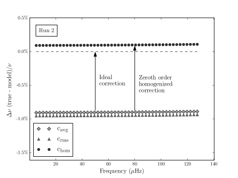
Figure 2.— Relative frequency differences as obtained in Run $2$, where the markers represent the same quantity as Figure 1. Run 2 corresponds to a higher Mach number than Run 1, and we find that the 0-th order homogenized approximation is not as effective at reproducing the true dispersion relation as in Run 1.

	$\left(\Delta\nu\right)_{\mathrm{avg}}$ (Run $1$)	$\left(\Delta\nu\right)_{\mathrm{avg}}$ (Run $2$)	$\left(\Delta\nu\right)_{\mathrm{avg}}$ (Run $3$)	$\left(\Delta\nu\right)_{\mathrm{avg}}$ (Run $4$)
$\omega=c_{\mathrm{hom}}k$	$0.009\,\mu\mathrm{Hz}$	$0.07\,\mu\mathrm{Hz}$	$-0.5\,\mu\mathrm{Hz}$	$0.29\,\mu\mathrm{Hz}$
$\omega=\langle c\rangle k$	$-0.15\,\mu\mathrm{Hz}$	$-0.59\,\mu\mathrm{Hz}$	$-1.8\,\mu\mathrm{Hz}$	$-1.36\,\mu\mathrm{Hz}$
$\omega=\sqrt{\langle c^{2}\rangle}k$	$-0.16\,\mu\mathrm{Hz}$	$-0.62\,\mu\mathrm{Hz}$	$-1.9\,\mu\mathrm{Hz}$	$-1.40\,\mu\mathrm{Hz}$

Table 2Comparison between the frequency differences corresponding to the different dispersion relation, averaged over the range $4\,\mu\mathrm{Hz}\leq\nu\leq 120\,\mu\mathrm{Hz}$. The homogenized relation, which accounts for flows explicitly, comes closest to the true dispersion relation.

5. Impact on solar frequencies

Correcting the solar oscillation equations involves correcting for both modal and model effects, as described by Rosenthal et al. (1999). In a recent paper, Piau et al. (2014) have explored the impact of various parametrization of stellar convection — from mixing-length theory (Spruit, 1977) to patched hydrodynamic models — on oscillation frequencies. They have used horizontally-averaged sound speeds from these models in the wave equation. We have shown that the presence of flows introduces further advective corrections in the wave speed, and the horizontally-averaged sound speeds do not represent the true wave speed. The actual speed of the waves is obtained from Equation (24), and the difference between this speed and the horizontally-averaged sound speed can be substantial near the solar surface.

In this section, we start from Model S (Christensen-Dalsgaard et al., 1996) which uses the mixing-length formulation of convective flux. We correct wave speeds using flow profiles obtained from simulations by Schüssler (personal communication) using the MURaM code (Vögler et al., 2005). The flow-speed profiles have been plotted in Figure 3. We start from equation (24) and work with low-degree modes $\left(\ell\leq 3\right)$, which are predominantly radial. We assume that the Mach number is low enough for the zeroth-order homogenization approximation (Equation 31) to hold, and retain only the dominant component of $\tilde{\mathbf{C}}$ which goes roughly as $c^{2}-u^{2}$. The exact form of $u$ which goes into the correction depends on the direction of advection at every depth; for our purpose we shall restrict ourselves to the special cases of radial flow $\left(\mathbf{u}={\bf u}_{\parallel}\right)$ and tangential flow $\left(\mathbf{u}={\bf u}_{\perp}\right)$. We refer to this modified model as Model Hom, and compute the eigenfrequencies corresponding to this model assuming the same boundary conditions as Model S. We compare these frequencies with observed solar frequencies obtained by the Birmingham Solar Oscillation Network (BiSON) (Chaplin et al., 2007). We find that the presence of flow advection in the wave equation leads to a reduction in mode frequencies, which reduces the observed difference between observed and Model S frequencies.

To study the impact of modal versus model corrections on frequencies, we compare the Model Hom frequencies with another hydrostatic model (Basu & Antia, 1994, henceforth called Model BA), which uses the Canuto-Mazzitelli formulation of convective flux (Canuto & Mazzitelli, 1991). The frequency differences between these models and the observations by BiSON have been plotted in Figure 4. We find that the modal frequency shifts due to the presence of advective flows is comparable to those obtained from modeling differences. Both the effects need to be looked into while fitting solar frequencies.

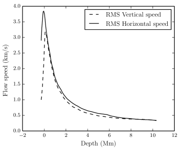
Figure 3.— Root-mean-square flow speeds obtained from three-dimensional simulation of the near-surface layers of the Sun (Vögler et al., 2005).

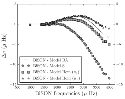
Figure 4.— Eigenfrequencies corresponding to Model S (Christensen-Dalsgaard et al., 1996, circles) compared with the modified models. The squares indicate a model where advection is predominantly radial and the stars indicate a model where advection is predominantly tangential. The dotted line represents eigenfrequencies corresponding to Model BA (Basu & Antia, 1994). We find that the modified models display frequency shifts comparable to Model BA, which shows that modal effects can be significant near the surface and need to be taken into account.

Some of the assumptions made in this section, such as diagonally-dominated and isotropic $\tilde{\mathbf{C}}$, are expected to be violated considerably near the surface, but the present example demonstrates that the effect of flow correction can be substantial. A detailed computation, starting either from a fully hydrodynamic background or a patched hydrodynamic background, is necessary to make quantitative statements about frequency shifts due to convective flows.

6. Conclusion

Observed solar oscillation frequencies can differ from modeled frequencies because of an inaccurate background model, as well as incomplete description of mode physics. The presence of near-surface convective flows on the Sun results in mode frequencies which are different from ones computed starting from a quiet background. Three-dimensional convection simulations generally result in an increased size of the acoustic cavity, thereby reducing the frequencies (Rosenthal et al., 1999; Piau et al., 2014). In this paper, we have shown that the impact of advection on waves might result in frequency shifts of similar magnitudes. In presence of flows, the appropriate wave speed is not the horizontally-averaged sound speed, rather it is a combination of sound speed and an appropriate projection of the flow speed in the direction of propagation.

Granulation length scales on the solar surface are much smaller than horizontal wavelengths corresponding to low-$\ell$ modes, which lets us replace the irregular background medium by an effective, homogeneous one. Acoustic waves propagating through steady background flows experience a change in phase speed on being scattered by the flows. The effective wave equation in the large-wavelength approximation has the form

$$\langle\rho\rangle\partial_{t}^{2}\bm{\xi_{0}}-\bm{\nabla}\cdot\left[\langle\rho\tilde{\mathbf{C}}\rangle:\bm{\nabla}\bm{\xi_{0}}\right]+\bm{\xi_{0}}\cdot\langle\rho\bm{\nabla}\bm{\nabla}\phi\rangle=\bm{0},$$

where the effective speed $\tilde{\mathbf{C}}$ is a tensor, given by Equation (22).

The impact of time evolution of flows, missing in the present analysis, needs to be studied in detail. The spatial scales of waves and background flows are significantly different, thereby allowing a two scale analysis. The timescales of granule evolution are, however, not very different from time periods of the wave. Overlap of scales generally results in strong scattering and forcing, thus a picture of flows evolving in time might be necessary to capture frequency shifts and damping. Added to this are the impact of super-adiabaticity and magnetic fields, which have been ignored in the present analysis, but might be important in governing the spectrum. Nevertheless the present analysis provides a useful starting point to model wave propagation through convective flows and resultant frequency shifts.

7. Acknowledgment

We thank the anonymous referee for his useful suggestions which improved the quality of this work significantly. JB would like to acknowledge the financial support provided by the Department of Atomic Energy, India.

References

- Auvergne et al. (2009) Auvergne, M., Bodin, P., Boisnard, L., et al. 2009, A&A, 506, 411
- Ball & Gizon (2014) Ball, W. H., & Gizon, L. 2014, ArXiv e-prints, arXiv:1408.0986
- Basu & Antia (1994) Basu, S., & Antia, H. M. 1994, Journal of Astrophysics and Astronomy, 15, 143
- Bensoussan et al. (1978) Bensoussan, A., Lions, J., & Papanicolaou, G. 1978, Asymptotic analysis for periodic structures (North-Holland Publishing Company)
- Borucki et al. (2010) Borucki, W. J., Koch, D., Basri, G., et al. 2010, Science, 327, 977
- Brown (1984) Brown, T. M. 1984, Science, 226, 687
- Canuto & Mazzitelli (1991) Canuto, V. M., & Mazzitelli, I. 1991, ApJ, 370, 295
- Chaplin et al. (2007) Chaplin, W. J., Elsworth, Y., Miller, B. A., Verner, G. A., & New, R. 2007, ApJ, 659, 1749
- Christensen-Dalsgaard et al. (1996) Christensen-Dalsgaard, J., Dappen, W., Ajukov, S. V., et al. 1996, Science, 272, 1286
- Duvall et al. (1998) Duvall, Jr., T. L., Kosovichev, A. G., & Murawski, K. 1998, ApJ, 505, L55
- Gough (1990) Gough, D. O. 1990, in Lecture Notes in Physics, Berlin Springer Verlag, Vol. 367, Progress of Seismology of the Sun and Stars, ed. Y. Osaki & H. Shibahashi, 283
- Hanasoge et al. (2013) Hanasoge, S. M., Gizon, L., & Bal, G. 2013, ApJ, 773, 101
- Kjeldsen et al. (2008) Kjeldsen, H., Bedding, T. R., & Christensen-Dalsgaard, J. 2008, ApJ, 683, L175
- Murawski & Roberts (1993) Murawski, K., & Roberts, B. 1993, A&A, 272, 595
- Papanicolaou & Varadhan (1982) Papanicolaou, G. C., & Varadhan, S. R. 1982, Statistics and probability: essays in honor of C. R. Rao, 547
- Piau et al. (2014) Piau, L., Collet, R., Stein, R. F., et al. 2014, MNRAS, 437, 164
- Rosenthal et al. (1999) Rosenthal, C. S., Christensen-Dalsgaard, J., Nordlund, Å., Stein, R. F., & Trampedach, R. 1999, A&A, 351, 689
- Spruit (1977) Spruit, H. C. 1977, PhD thesis, Thesis University of Utrecht, The Netherlands.
- Stix & Zhugzhda (2004) Stix, M., & Zhugzhda, Y. D. 2004, A&A, 418, 305
- Vögler et al. (2005) Vögler, A., Shelyag, S., Schüssler, M., et al. 2005, A&A, 429, 335
- Webb et al. (2005) Webb, G. M., Zank, G. P., Kagashvili, E. K., & Ratkiewicz, R. E. 2005, Journal of Plasma Physics, 71, 785