Revisiting slow-roll inflation in nonminimal derivative coupling with potentials

Abstract

We investigate the slow-roll inflation in the nonminimal derivative coupling (NDC) model with exponential, quadric, and quartic potentials. It was known that this model provides an enhanced slow-roll inflation induced by gravitationally enhanced friction even for a steep exponential potential. In the phase portrait, the inflationary attractor is described by the slow-roll equation. Introducing the autonomous form, the inflation is regarded as an emergence from the saddle point and it leaves this fixed point along the slow-roll equation. We show explicitly that if one uses the NDC with potentials, the slow-roll inflation is easier to be implemented than the canonical coupling with the same potentials.

1 Introduction

The nonminimal derivative coupling (NDC) [1, 2] was achieved by coupling the inflaton kinetic term to the Einstein tensor such that the friction is enhanced gravitationally at higher energies [3]. This gravitationally enhanced friction mechanism is a powerful tool to increase friction of an inflaton rolling down its own potential without introducing new degrees of freedom unlike hybrid inflation. Actually, this NDC makes a steep (non-flat) potential adequate for inflation without possessing higher-time derivative terms (ghost state) [4, 5]. It is well-known that the exponential potential provides a power-law inflation and thus, it cannot account for an inflationary theory since the inflation never ends and an additional mechanism is required to stop it [6]. The kinetic coupling flattens the potential effectively as well as it increases friction. Recently, this coupling allowed inflation to take place for a wide range of values $\lambda$ in the (non-flat) exponential potential $V=V_{0}e^{-\lambda\phi}$ which implies that it features a natural exit from inflation [7].

In this paper, we study the autonomous dynamical system of an homogeneous and isotropic configuration of a scalar field non minimally coupled to gravity, as in [8, 9, 10, 11, 12, 13, 14, 15, 16]. We found that in the two dimensional dynamical system of the field value and its derivative, the space of initial conditions providing inflationary attractors is larger in NDC than in the canonical case. Specifically we have investigated NDC models with exponential, quadric, and quartic potentials since non-flat potentials of exponential and quartic potentials with canonical coupling (CC) [17] are in tension with the Planck data [18]. Especially, the exponential potential is regarded as a testing potential because it could provide a power-law (eternal) inflation in the CC model while it could provide a slow-roll inflation in the NDC model [19].

2 An inflation model of NDC

Let us consider an inflation model whose action includes NDC of scalar field $\phi$ with a potential term [3, 4, 5, 20]

$$S=\frac{1}{2}\int d^{4}x\sqrt{-g}\Big{[}M_{\rm P}^{2}R+\frac{1}{\tilde{M}^{2}}G_{\mu\nu}\partial^{\mu}\phi\partial^{\nu}\phi-2V(\phi)\Big{]},$$ (2.1)

where $M_{\rm P}$ is a reduced Planck mass, $\tilde{M}$ is a mass parameter, and $G_{\mu\nu}=R_{\mu\nu}-g_{\mu\nu}R/2$ is the Einstein tensor. Here, we do not include a canonical coupling (CC) term like as a conventional combination of $(g_{\mu\nu}-G_{\mu\nu}/\tilde{M}^{2})\partial^{\mu}\phi\partial^{\nu}\phi$ [19, 21] because this combination won’t make the analysis transparent (see Appendix A for the autonomous system for CC+NDC).

Varying the action (2.1) with respect to the metric tensor $g_{\mu\nu}$ leads to the Einstein equation

$$G_{\mu\nu}=\frac{1}{M_{\rm P}^{2}}T_{\mu\nu}^{\rm NDC},$$ (2.2)

where $T_{\mu\nu}^{\rm NDC}$ takes the complicated form

$$T_{\mu\nu}^{\rm NDC} = \frac{1}{\tilde{M}^{2}}\Big{[}\frac{1}{2}R\nabla_{\mu}\phi\nabla_{\nu}\phi-2\nabla_{\rho}\phi\nabla_{(\mu}\phi R_{\nu)}^{\rho}+\frac{1}{2}G_{\mu\nu}(\nabla\phi)^{2}-R_{\mu\rho\nu\sigma}\nabla^{\rho}\phi\nabla^{\sigma}\phi$$ (2.3)

$$\hskip 50.00008pt-\nabla_{\mu}\nabla^{\rho}\phi\nabla_{\nu}\nabla_{\rho}\phi+(\nabla_{\mu}\nabla_{\nu}\phi)\nabla^{2}\phi$$

$$-g_{\mu\nu}\Big{(}-R^{\rho\sigma}\nabla_{\rho}\phi\nabla_{\sigma}\phi+\frac{1}{2}(\nabla^{2}\phi)^{2}-\frac{1}{2}(\nabla^{\rho}\nabla^{\sigma}\phi)\nabla_{\rho}\nabla_{\sigma}\phi\Big{)}\Big{]}.$$

Here, we note that even though fourth-order derivative terms are present in $T^{\rm NDC}_{\mu\nu}$, there is no ghost state which means that any higher-time derivative term more than two is not generated. On the other hand, the scalar equation is derived to be

$$-\frac{1}{\tilde{M}^{2}}G^{\mu\nu}\nabla_{\mu}\nabla_{\nu}\phi-V^{\prime}=0,$$ (2.4)

where the prime (^′) denotes derivative with respect to $\phi$.

In this work, we consider a spatially flat spacetime by introducing cosmic time $t$ as

$$ds^{2}~{}=~{}\bar{g}_{\mu\nu}dx^{\mu}dx^{\nu}~{}=~{}-dt^{2}+a^{2}(t)\delta_{ij}dx^{i}dx^{j},$$ (2.5)

where $a(t)$ is a scale factor. In this spacetime, two Friedmann equations and scalar equation become

$$H^{2} = \frac{1}{3M_{\rm P}^{2}}\Big{[}\frac{9H^{2}}{2\tilde{M}^{2}}\dot{\phi}^{2}+V\Big{]},$$ (2.6)

$$\dot{H} = -\frac{1}{2M_{\rm P}^{2}}\Big{[}\dot{\phi}^{2}\Big{(}\frac{3H^{2}}{\tilde{M}^{2}}-\frac{\dot{H}}{\tilde{M}^{2}}\Big{)}-\frac{2H}{\tilde{M}^{2}}\dot{\phi}\ddot{\phi}\Big{]},$$ (2.8)

$$\frac{3H^{2}}{\tilde{M}^{2}}\ddot{\phi}+3H\Big{(}\frac{3H^{2}}{\tilde{M}^{2}}+\frac{2\dot{H}}{\tilde{M}^{2}}\Big{)}\dot{\phi}+V^{\prime}=0,$$

where $H=\dot{a}/a$ is the Hubble parameter and the overdot ($\dot{}$) denotes derivative with respect to time $t$. We observe from (2.6) that the energy density for the NDC is positive (ghost-free) [22].

Now we define two slow-roll parameters as

$$\epsilon_{N}=-\frac{\dot{H}}{H^{2}},~{}~{}~{}~{}~{}\delta_{N}=\frac{\ddot{\phi}}{H\dot{\phi}}.$$ (2.9)

Imposing slow-roll conditions ($\epsilon_{N}\ll 1,~{}\delta_{N}\ll 1$), Eqs. (2.6)-(2.8) can be written approximately as

$$H^{2} \simeq \frac{1}{3M_{\rm P}^{2}}V,$$ (2.10)

$$\dot{H} \simeq -\frac{3H^{2}}{2M_{\rm P}^{2}\tilde{M}^{2}}\dot{\phi}^{2},$$ (2.11)

$$3H\dot{\phi} \simeq -\frac{\tilde{M}^{2}}{3H^{2}}V^{\prime}.$$ (2.12)

We note that the slow-roll parameter $\epsilon_{N}$ can be written as

$$\epsilon_{N}~{}\simeq~{}\epsilon_{N}^{V}~{}\simeq~{}\epsilon_{N}^{H},$$ (2.13)

where the potential $\epsilon_{N}^{V}$ and Hubble slow-roll parameters $\epsilon_{N}^{H}$ are given by [4, 23]

$$\epsilon_{N}^{V}=\frac{M_{\rm P}^{2}\tilde{M}^{2}}{6}\frac{V^{\prime 2}}{V^{2}H^{2}},~{}~{}~{}~{}~{}\epsilon_{N}^{H}=\frac{3}{2M_{\rm P}^{2}\tilde{M}^{2}}\dot{\phi}^{2}.$$ (2.14)

The end of inflation can be identified with the end of slow-roll regime. Therefore, we may define the value of field at the end of inflation $\phi_{f}$ by making use of $\epsilon^{V}_{N}=1$.

3 Dynamical analysis

In this section, we wish to perform the dynamical analysis for (2.6)-(2.8). For this purpose, one introduces with some dimensionless quantities and obtains their autonomous system. Before we proceed, it is instructive to investigate the canonical coupling (CC) model for comparison and exercise.

3.1 Analysis of CC models

In this case, the corresponding field equations are given by

$$H^{2} = \frac{1}{3M_{\rm P}^{2}}\Big{[}\frac{1}{2}\dot{\phi}^{2}+V\Big{]},$$ (3.1)

$$\dot{H} = -\frac{1}{2M_{\rm P}^{2}}\dot{\phi}^{2},$$ (3.3)

$$\ddot{\phi}+3H\dot{\phi}+V^{\prime}=0.$$

It is well-known that in the slow-roll approximation, they reduce to

$$H^{2} \simeq \frac{V}{3M_{\rm P}^{2}},$$ (3.4)

$$\dot{H} = -\frac{1}{2M_{\rm P}^{2}}\dot{\phi}^{2},$$ (3.5)

$$3H\dot{\phi} \simeq -V^{\prime},$$ (3.6)

which are obtained by imposing slow-roll condition of $\epsilon_{C}=-\dot{H}/H^{2}\ll 1$ and $\delta_{C}=\ddot{\phi}/H\dot{\phi}\ll 1$. Here we have $\epsilon_{C}\simeq\epsilon_{C}^{V}\simeq\epsilon_{C}^{H}$ with

$$\epsilon_{C}^{V}\equiv\frac{M_{\rm P}^{2}}{2}\frac{V^{\prime 2}}{V^{2}},~{}~{}~{}~{}~{}\epsilon_{C}^{H}\equiv\frac{\dot{\phi}^{2}}{2M_{\rm P}^{2}H^{2}}.$$ (3.7)

We note that the NDC parameters of $\epsilon^{V,H}_{N}$ (2.14) are slightly different from the CC parameters $\epsilon^{V,H}_{C}$ (3.7). In particular, $\epsilon^{V}_{N}=\epsilon^{V}_{C}\times\tilde{M}^{2}/(3H^{2})$ implies that when $\tilde{M}^{2}/(3H^{2})\ll 1$, inflation in the NDC can happen more easily than the CC case.

To perform the dynamical analysis for the cosmological evolution equations (3.1)-(3.3), we consider the dimensionless variables

$$x\equiv\frac{\dot{\phi}}{M_{\rm P}\sqrt{6}H},~{}~{}~{}y\equiv\frac{\sqrt{V}}{M_{\rm P}\sqrt{3}H},~{}~{}~{}\alpha_{V}\equiv\sqrt{6}M_{\rm P}\frac{V^{\prime}}{V},~{}~{}~{}\Gamma\equiv\frac{VV^{\prime\prime}}{V^{\prime 2}}.$$ (3.8)

The connections between $(x,\alpha_{V})$ and ($\epsilon^{H}_{C},\epsilon^{V}_{C}$) are given by

$$x^{2}=\frac{\epsilon_{C}^{H}}{3},~{}~{}\alpha^{2}_{V}=12\epsilon_{C}^{V}.$$ (3.9)

Then, the first Friedmann equation (3.1) becomes a constraint equation

$$x^{2}+y^{2}=1,$$ (3.10)

which implies that the variable $y$ can be eliminated from the dynamical equations.

It is found that (3.1)-(3.3) lead to the autonomous form for ${\bf X}=(x,\alpha_{V})$

$$\frac{dx}{dN} = 3(x^{2}-1)\Big{(}x+\frac{\alpha_{V}}{6}\Big{)},$$ (3.11)

$$\frac{d\alpha_{V}}{dN} = \alpha_{V}^{2}x(\Gamma-1)$$ (3.12)

with $N=\ln a$. Fixed points of first-order autonomous system are given by $dx/dN=0$ and $d\alpha_{V}/dN=0$. By a fixed point we mean that $x$ and $\alpha_{V}$ do not change as the universe evolves. Perturbing these points leads to stable point (attractor), saddle point, and unstable point (repeller). Then, one can classify these according to their eigenvalue solution to perturbed equations: all negative (stable point); all positive (unstable), different signs (saddle point).

At this stage, it is worth noting that the slow-roll trajectory can be found by considering two different ways: One is found by solving the slow-roll equations (3.4)-(3.6) and the other is found by solving the autonomous system (3.11) and (3.12) in the slow-roll approximation. The former indicates an inflationary attractor in phase portrait $(\phi,\dot{\phi})$, while the latter shows that inflation is regarded as “an emergence from the saddle point and it can leave this fixed point along the slow-roll equation”. For this purpose, we introduce three potentials: exponential, quadric (chaotic), and quartic potentials. The first one is regarded as a testing potential because it cannot provide a slow-roll inflation in the CC model, whereas it could provide a slow-roll inflation in the NDC model.

We should distinguish between inflationary attractor in ($\phi,\dot{\phi}$) and attractor of stable fixed point in ($x,\alpha_{V}$). To this end, we note that slow-roll equations (3.4)-(3.6) are combined to give

$$\dot{\phi}\simeq-M_{\rm P}^{2}\frac{HV^{\prime}}{V},$$ (3.13)

which describes an inflationary attractor. This can be expressed in terms of $x$ and $\alpha_{V}$ defined in (3.8) as

$$x\simeq-\frac{\alpha_{V}}{6}.$$ (3.14)

We note that Eq.(3.14) satisfies $\epsilon_{C}^{H}\simeq\epsilon_{C}^{V}$ which yields $x^{2}\simeq\alpha_{V}^{2}/36$, when substituting (3.9) into $\epsilon_{C}^{H,V}$. Also, (3.14) describes a slow-roll line solution to an approximate equation

$$\frac{dx}{dN} \simeq x+\frac{\alpha_{V}}{6}\simeq 0,$$ (3.15)

which was found from (3.11) by taking into account the slow-roll condition of $\epsilon_{C}^{H}=3x^{2}\ll 1$. This implies that any fixed point can be defined only for $\Gamma=1$ ($\alpha_{V}$=const) or $x=0$ ($\alpha_{V}$=0), while the slow-roll line is defined without imposing $\alpha_{V}$=const. Here, a slow-roll line is given by a function [$\alpha_{V}(x)=-6x$] which exists during inflation. Hence, we identify the inflationary attractor in phase portrait ($\phi,\dot{\phi}$) with the slow-roll line (equation) in stream flow ($x,\alpha_{V}$). The slow-roll approximation reduces the order of the system equations by one and thus, its general solution contains one less initial condition. It works only because the solution to the full equations has an attractor property eliminating the dependence on the extra parameter.

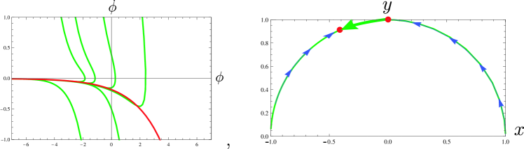
Figure 1: The phase portrait $(\phi,\dot{\phi})$ [left] and stream flow $(x,y)$ [right] for $V=V_{0}e^{\lambda\phi}$ with $V_{0}=0.1$, $\lambda=1$ and $M_{\rm P}=1$. Left panel shows the trajectories (green curves) with various initial conditions toward the inflationary attractor (red curve). This red curve is mapped into a fixed point of red dot at $(-0.408,0.912)$ in the right panel. This corresponds to a stable fixed point (attractor), while the point (0,1) denotes a saddle point. The green curves in the left are mapped on the green curves on the upper circle in the right.

For complete analysis, we choose an explicit potential.

$(i)~{}V=V_{0}e^{\lambda\phi}$

For an exponential potential, the inflaton velocity (3.13) is given by

$$\dot{\phi}\simeq-M_{\rm P}\lambda\sqrt{\frac{V_{0}}{3}}e^{\frac{\lambda}{2}\phi}.$$ (3.16)

Solving (3.1)-(3.3) numerically for various initial conditions, they show the trajectories. Also, the slow-roll equation (3.16) may indicate an inflationary trajectory [see Fig.1 (left)]. However, this case corresponds to $\epsilon_{C}^{V}=M^{2}_{\rm P}/2$ (power-law inflation), implying that it cannot be a complete inflationary model because inflation never ends with the potential $V=V_{0}e^{\lambda\phi}$. In order to see it more clearly, we have to know what happens in the stream plot where fixed points are included naturally. In this case, we have $\Gamma=1(\alpha_{V}$=const). Therefore, we could not make a stream flow on $(x,\alpha_{V})$. Instead, we have the stream flow on ($x,y$). We find a corresponding fixed point of $(x,y)=(-\alpha_{V}/6,\sqrt{1-\alpha_{V}^{2}/36})=(-0.408,0.912)$ in Fig.1 (right) which turns out to be an attractor (stable fixed point), in addition to the (0,1)-saddle point. Clearly, it indicates that the potential $V=V_{0}e^{\lambda\phi}$ in the CC model cannot provide a complete slow-roll inflation because power-law inflation never ends. This means that there is no spiral sink which indicates the end of inflation in the left of Fig. 1.

$(ii)~{}V=V_{0}\phi^{2}$

In the case of chaotic potential, the inflationary attractor (3.13) is given by

$$\dot{\phi}\simeq\left\{\begin{array}[]{ll}-2M_{\rm P}\sqrt{\frac{V_{0}}{3}},~{}~{}(\phi>0)\\ +2M_{\rm P}\sqrt{\frac{V_{0}}{3}},~{}~{}(\phi<0)\end{array}\right.,$$ (3.19)

which corresponds to a positive (negative) constant $\dot{\phi}$-line for $\phi<0$ ($\phi>0$) in the ($\phi,\dot{\phi}$) picture.

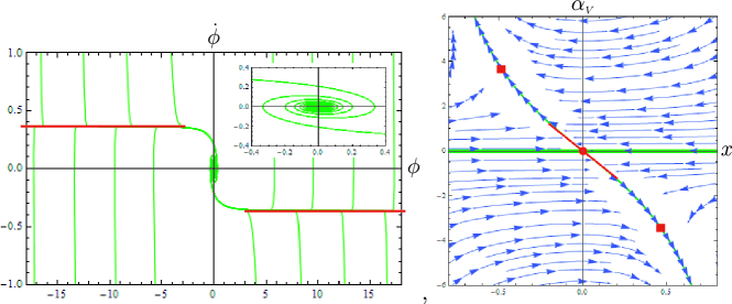
Figure 2: The phase portrait $(\phi,\dot{\phi})$ [left] and stream flow $(x,\alpha_{V})$ [right] for $V=V_{0}\phi^{2}$ with $V_{0}=0.1$ and $M_{\rm P}=1$. Left panel shows the trajectories toward the inflationary attractor (red lines) for $\phi\lessgtr 0$ including a spiral sink. These red lines correspond to a red line of $\alpha_{V}=-6x$ in the right panel. Also, the green flows in the right show the numerical plot for ($x,\alpha_{V}$) when using (3.1)-(3.3). These flows indicate that the inflation is emergent from the saddle point ($\bullet$) (0,0) and is realized along the red line. Finally, the inflation ends at the point ($\blacksquare$) ($\mp 0.46,\pm 3.48$), corresponding to $\epsilon_{C}^{V}=1$.

Figure 2 shows a typical picture based on numerical computation. When the universe evolves according to (3.1)-(3.3) and (3.11)-(3.12), the inflationary attractor and slow-roll line are given by (3.19) in the phase portrait ($\phi,\dot{\phi}$) [Fig.2 (left) panel] [13, 14, 6] and (3.14) in stream flow ($x,\alpha_{V}$) [Fig.2 (right) panel], respectively. There are three phases in the CC case [24]: initially, kinetic energy dominates and due to the rapid decrease of the kinetic energy the trajectory runs quickly to the inflationary attractor line (3.19). All initial trajectories are attracted to this line, which is the key feature of slow-roll inflation. Finally, at the end of inflation, there is inflaton decay and reheating (spiral sink).

On the other hand, the inflation can be realized as an emergence from the potential-dominated fixed point $(0,0)$ which is a saddle point because orbits near it are attracted along one direction and repelled along another direction. The stream flows in the right of Fig. 2 can leave this fixed point only along the red line of $\alpha_{V}=-6x$ corresponding to the slow-roll line (3.14) and the inflation ends at the point ($\mp 0.46,\pm 3.48$), which corresponds to $\epsilon_{C}^{V}=1$ with $\alpha_{V}=\pm 3.48$. We note here that $x$-axis is the stable manifold of the saddle point, while $\alpha_{V}=-6x$ is the unstable manifold of the saddle point.

$(iii)~{}V=V_{0}\phi^{4}$

The inflationary attractor (3.13) for this case is given by

$$\dot{\phi}\simeq-4M_{\rm P}\sqrt{\frac{V_{0}}{3}}\phi.$$ (3.20)

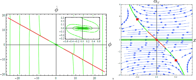
Figure 3: The phase portrait $(\phi,\dot{\phi})$ [left] and stream flow $(x,\alpha_{V})$ [right] for $V=V_{0}\phi^{4}$ with $V_{0}=0.1$, $M_{\rm P}=1$. Left panel shows the trajectories toward the inflationary attractor (red lines) followed by spiral sink. These lines correspond to a red line of $\alpha_{V}=-6x$ in the right panel. Also, the green flows in the right show the numerical plot for ($x,\alpha_{V}$) when using (3.1)-(3.3). These flows indicate that the inflation is emergent from the saddle point ($\bullet$) (0,0) and is realized along the red line. Finally, the inflation ends at the point ($\blacksquare$) ($\mp 0.50,\pm 3.48$), which corresponds to $\epsilon_{C}^{V}=1$.

Figure 3 shows that when solving (3.1)-(3.3) and (3.11)-(3.12) numerically, the inflationary attractor (decreasing function) is given by the slow-roll equation (3.20) followed by a spiral sink in the phase portraits ($\phi,\dot{\phi}$) [Fig.3 (left)] and the red line (3.14) in stream flows ($x,\alpha_{V}$) [Fig.3 (right)], respectively. Inflation can be realized as an emergence from the saddle point $(0,0)$. The inflation can leave this fixed point only along the red line of $\alpha_{V}=-6x$ corresponding to the slow-roll line (3.14) and it ends at the point ($\mp 0.50,\pm 3.48$), which corresponds to $\epsilon_{C}^{V}=1$ with $\alpha_{V}=\pm 3.48$.

3.2 Analysis of NDC models

Now we turn to the NDC case. To perform the dynamical analysis for (2.6)-(2.8), we consider the dimensionless parameters $u$ and $\alpha_{u}$ in addition to $y$ and $\Gamma$ defined in (3.8)

$$u\equiv\sqrt{\frac{3}{2}}\frac{\dot{\phi}}{M_{\rm P}\tilde{M}},~{}~{}~{}\alpha_{u}=\sqrt{6}\frac{M_{\rm P}\tilde{M}V^{\prime}}{VH}.$$ (3.21)

The connections between $(u,\alpha_{u})$ and ($\epsilon^{H}_{N},\epsilon^{V}_{N}$) are given by

$$u^{2}=\epsilon_{N}^{H},~{}~{}\alpha^{2}_{u}=36\epsilon_{N}^{V}.$$ (3.22)

Then, the constraint equation (2.6) becomes

$$u^{2}+y^{2}=1,$$ (3.23)

which implies that one may eliminate $y$ from the dynamical equations. It turns out that (2.6)-(2.8) lead to the autonomous form for ${\bf X}=(u,\alpha_{u})$

$$\frac{du}{dN} = (2\epsilon_{N}-3)u-\frac{1}{2}\alpha_{u}(1-u^{2}),$$ (3.24)

$$\frac{d\alpha_{u}}{dN} = \epsilon_{N}\alpha_{u}+\frac{1}{3}(\Gamma-1)u\alpha_{u}^{2},$$ (3.25)

where $\epsilon_{N}=-\dot{H}/H^{2}$ satisfies the relation

$$(1+u^{2})\epsilon_{N}=3u^{2}+\frac{1}{3}\alpha_{u}u(1-u^{2}).$$ (3.26)

On the other hand, we note that slow-roll equations (2.10)-(2.12) give us the inflaton velocity

$$\dot{\phi}\simeq-M_{\rm P}^{2}\tilde{M}^{2}\frac{V^{\prime}}{3HV},$$ (3.27)

which corresponds to

$$u\simeq-\frac{\alpha_{u}}{6}.$$ (3.28)

We note that Eq.(3.28) satisfies $\epsilon_{N}^{H}\simeq\epsilon_{N}^{V}$ which yields $u^{2}\simeq\alpha_{u}^{2}/36$, when substituting (3.22) into $\epsilon_{N}^{H,V}$. Also, it is worth to mention that Eq.(3.28) corresponds to Eq.(3.14) in CC. Furthermore, Eq.(3.28) can be realized as a slow-roll line solution to (3.24) when implementing slow-roll condition of $\epsilon_{N}^{H}=u^{2}\ll 1$ which takes the form

$$\frac{du}{dN} \simeq -3u-\frac{\alpha_{u}}{2}\simeq 0.$$ (3.29)

Differing with the CC model, there exists an upper limit of $\dot{\phi}^{2}$

$$0<\dot{\phi}^{2}<\phi_{c}^{2}\equiv\frac{2}{3}M_{\rm P}^{2}\tilde{M}^{2},$$ (3.30)

which comes from Eq.(2.6) yielding $H^{2}(1-\dot{\phi}^{2}/\phi^{2}_{c})=V/3M^{2}_{\rm P}$ where the left-handed side should be positive for a positive potential. This may be regarded as another representation of slow-roll condition ($\epsilon^{H}_{N}=u^{2}\ll 1$).

,

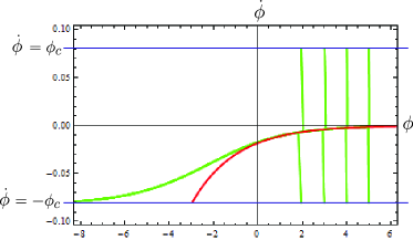
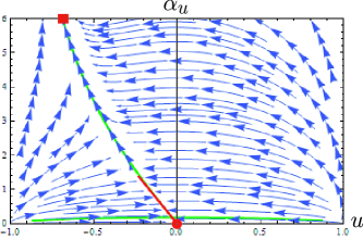
Figure 4: The phase portrait $(\phi,\dot{\phi})$ [left] and stream flow $(u,\alpha_{u})$ [right] for $V=V_{0}e^{\lambda\phi}$ with $V_{0}=0.1$, $\lambda=1$, $M_{\rm P}=1$, $\tilde{M}=0.1$, and $\phi_{c}=M_{\rm P}\tilde{M}\sqrt{2}/{\sqrt{3}}\simeq 0.08$. Left panel shows the trajectories toward the inflationary attractor (red curve). Here is no stable limited cycle. This curve corresponds to a red line of $\alpha_{u}=-6u$ in the right panel. Also, the green flows in the right show the numerical plot for ($u,\alpha_{u}$) when using (2.6)-(2.8). These flows show that inflation is emergent from the saddle point ($\bullet$) (0,0) and is realized along the red line. Finally, the inflation ends at the point ($\blacksquare$) ($-0.69,6$), which corresponds to $\epsilon_{N}^{V}=1$.

Now, we solve (2.6)-(2.8) and (3.24)-(3.25) numerically by considering three of exponential, quadric (chaotic), and quartic potentials.

$(i)~{}V=V_{0}e^{\lambda\phi}$

For an exponential potential, the inflaton velocity (3.27) is given by

$$\dot{\phi}\simeq-\frac{M_{\rm P}^{3}\tilde{M}^{2}\lambda}{\sqrt{3V_{0}}}e^{-\frac{\lambda}{2}\phi},$$ (3.31)

which implies that when solving (2.6)-(2.8) numerically for various initial conditions, any solution should attract the trajectory of (3.31) [see Fig.4 (left)]. Here we note that there is no spiral sink because the potential approaches zero in the limit of $\phi\to-\infty$. We point out that $\alpha_{u}=-6u$ (3.28) cannot be an attractor (point) because of evolution of $H$ in $\alpha_{u}$ (3.21) even though $V^{\prime}/V=\lambda$. This contrasts to the CC case, which yields an attractor (point) at $x=-\alpha_{V}/6$ for the exponential potential [see Fig.1 (right)] implying that the slow-roll never ends.

On the other hand, for the NDC case with the exponential potential, one checks that the inflationary attractor in the ($u,\alpha_{u}$) is given by a slow-roll line of $\alpha_{u}=-6u$ [see Fig.4 (right)]. In this case, inflation can be realized as an emergence from the saddle point $(0,0)$. The stream flows in the right of Fig. 4 can leave the point $(0,0)$ only along the red line of $u=-\alpha_{u}/6$ corresponding to the slow-roll line (3.28) and the inflation ends at the point ($-0.69,6$), which corresponds to $\epsilon_{N}^{V}=1$ with $\alpha_{u}=6$.

$(ii)~{}V=V_{0}\phi^{2}$

In case of chaotic potential, the inflaton velocity (3.27) is given by

$$\dot{\phi}\simeq\left\{\begin{array}[]{ll}-\frac{2M_{\rm P}^{3}\tilde{M}^{2}}{\sqrt{3V_{0}}}\frac{1}{\phi^{2}},~{}~{}(\phi>0)\\ +\frac{2M_{\rm P}^{3}\tilde{M}^{2}}{\sqrt{3V_{0}}}\frac{1}{\phi^{2}},~{}~{}(\phi<0)\end{array}\right..$$ (3.34)

Figure 5 shows that when solving Eqs. (2.6)-(2.8) and (3.24)-(3.25) numerically, the inflationary attractors are given by the red curve (3.34) followed by stable limited cycle on ($\phi,\dot{\phi}$) [Fig.5 (left)] and the slow-roll line (3.28) starting at (0,0) [Fig.5 (right)]. We note here that the stable limited cycle where nearby curves spiral towards closed curve $C$ appears instead of the spinal sink in the CC. Hence, the trajectories trace out a closed curve $C$.

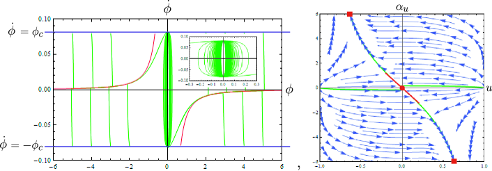
Figure 5: The phase portrait $(\phi,\dot{\phi})$ [left] and stream flow $(u,\alpha_{u})$ [right] for $V=V_{0}\phi^{2}$ with $V_{0}=0.1$, $M_{\rm P}=1$, $\tilde{M}=0.1$, and $\phi_{c}=M_{\rm P}\tilde{M}\sqrt{2}/{\sqrt{3}}\simeq 0.08$. Left panel shows the trajectories toward the inflationary attractor (red curves) followed by stable limited cycle. These curves correspond to a red line of $\alpha_{u}=-6u$ in the right panel. Also, the green flows in the right show the numerical plot for ($u,\alpha_{u}$) when solving (2.6)-(2.8). These flows indicate that the inflation is emergent from the saddle point $(\bullet)$ (0,0) and is realized along the red line. Finally, the inflation ends at the point ($\blacksquare$) ($\mp 0.63,\pm 6$), which corresponds to $\epsilon_{N}^{V}=1$.

Inflation can be realized as an emergence from the saddle point $(0,0)$. The stream flows in the right of Fig. 5 indicate that the inflation can leave the saddle point $(0,0)$ only along the red line of $u=-\alpha_{u}/6$ corresponding to the slow-roll line (3.28). The inflation ends at the point ($\mp 0.63,\pm 6$), which corresponds to $\epsilon_{N}^{V}=1$ with $\alpha_{u}=\pm 6$. Furthermore, comparing the red curve in Fig.5 (left) with the red line in Fig.2 (left) indicates that the NDC suppresses the kinetic term $\dot{\phi}$ whereas it enhances higher friction.

$(iii)~{}V=V_{0}\phi^{4}$

The inflaton velocity (3.27) for this case is given by

$$\dot{\phi}\simeq-\frac{4M_{\rm P}^{3}\tilde{M}^{2}}{\sqrt{3V_{0}}}\frac{1}{\phi^{3}}.$$ (3.35)

Finally, Figure 6 shows that when solving (2.6)-(2.8) and (3.24)-(3.25) numerically, the inflationary attractors are given by the red curve (3.35) followed by stable limited cycle on ($\phi,\dot{\phi}$) [Fig.6 (left)] and slow-roll line (3.28) on ($u,\alpha_{u}$) [Fig.6 (right)]. Inflation can be realized as an emergence from the saddle point $(0,0)$. The stream flows in the right of Fig. 6 indicate that inflation can leave the point $(0,0)$ only along the red line of $\alpha_{u}=-6u$ corresponding to the slow-roll line (3.28) and the inflation ends at the point ($\mp 0.66,\pm 6$), which corresponds to $\epsilon_{N}^{V}=1$ with $\alpha_{u}=\pm 6$. Also, comparing the red curve in Fig.6 (left) with the red curve in Fig.3 (left) indicates that the NDC suppresses the inflaton velocity $\dot{\phi}$ whereas it enhances higher friction. This means that the initial kinetic energy in the NDC is small when compared with the potential energy. On the other hand, the kinetic energy in the CC rapidly decreases until eventually the potential energy dominates and the universe may enter the slow-roll inflation. However, it is not easy to obtain an enough e-folds number from $\phi^{4}$ in the CC. This explains why this potential was ruled out [18].

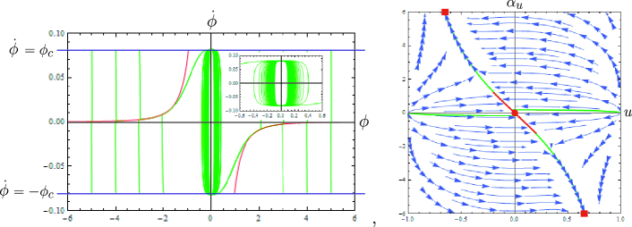
Figure 6: The phase portrait $(\phi,\dot{\phi})$ [left] and stream flow $(u,\alpha_{u})$ [right] for $V=V_{0}\phi^{4}$ with $V_{0}=0.1$, $M_{\rm P}=1$, $\tilde{M}=0.1$, and $\phi_{c}=M_{\rm P}\tilde{M}\sqrt{2}/{\sqrt{3}}\simeq 0.08$. Left panel shows the trajectories toward the inflationary attractor (red curves) followed by stable limited cycle. These curves correspond to a red line of $\alpha_{u}=-6u$ in the right panel. Also, the green flows in the right show the numerical plot for ($u,\alpha_{u}$) when using (2.6)-(2.8). This flow shows that the inflation is emergent from the saddle point $(\bullet)$ (0,0) and is realized along the red line. Finally, the inflation ends at the point ($\blacksquare$) ($\mp 0.66,\pm 6$), which corresponds to $\epsilon_{N}^{V}=1$.

4 Summary and Discussions

First of all, we compare the NDC with the CC with the same potentials. In the phase portrait ($\phi,\dot{\phi}$), the slow-roll inflation is identified with the presence of inflationary attractor (slow-roll equation) followed by spiral sink (0,0) (the ending of inflation) for the CC and stable limited cycle centered at (0,0) for the NDC. See Fig. 7 for the different behaviors of $\phi$ and $\dot{\phi}$ between the CC and NDC during the evolution of the universe. On the other hand, the corresponding autonomous forms for ${\bf X}$=($x(u),\alpha_{V(u)}$) indicated that the slow-roll inflation is realized by emerging a saddle point (0,0) (the beginning of inflation) and inflation leaves this point along the slow-roll equation. This is so because of $(x,\alpha_{V})\simeq(\dot{\ln[\phi]},\frac{1}{\phi})$ for $\phi^{2}$ and $(\frac{\dot{\phi}}{\phi^{2}},\frac{1}{\phi^{2}})$ for $\phi^{4}$ in the CC case. In the NDC case, $(u,\alpha_{u})\simeq(\dot{\phi},\frac{1}{\phi^{2}})$ and $(\dot{\phi},\frac{1}{\phi^{3}})$. This implies that even though the limit of $\phi\to 0$ is not implemented by the autonomous system, the other limit of $\phi\to\infty$ can be easily realized at the origin (0,0).

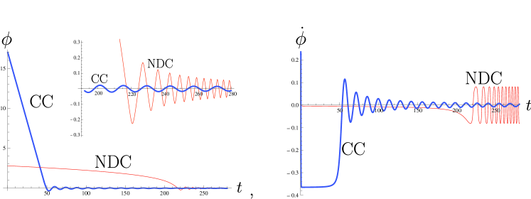
Figure 7: The evolution of $\phi(t)$ [left] and $\dot{\phi}(t)$ [right] with respect to time $t$ for potential $\phi^{2}$. The left figure shows that the inflaton varies little during large inflationary period for the NDC, while it varies quickly during small inflationary period for the CC. After inflation, $\phi$ decays with oscillation for CC, while it oscillates rapidly for NDC. The right one indicates that for large $t$, $\dot{\phi}$ oscillates without damping for the NDC, while it oscillates with damping for the CC.

We summarize our results in Table 1. $\phi_{i}$ is the value of $\phi$ when the phase space trajectory hits the inflationary attractor while $\phi_{f}$ is determined by $\epsilon_{C,N}^{V}=1$. The relations are given for the exponential ($e^{\lambda\phi}$) and power-law potential ($\phi^{n}$) by

$$\phi_{f}-\phi_{i}=-\lambda M_{\rm P}^{2}N~{}~{}~{}({\rm CC}), e^{\lambda\phi_{f}}-e^{\lambda\phi_{i}}=-\lambda^{2}M_{\rm P}^{4}\tilde{M}^{2}\frac{N}{V_{0}}~{}~{}~{}({\rm NDC})$$

$$\phi_{f}^{2}-\phi_{i}^{2}=-2M_{\rm P}^{2}nN~{}~{}~{}({\rm CC}), \phi_{f}^{n+2}-\phi_{i}^{n+2}=-n(n+2)M_{\rm P}^{4}\tilde{M}^{2}\frac{N}{V_{0}}~{}~{}~{}({\rm NDC}),$$

where the e-fold number is $N=70$. $\Delta\phi=\phi_{f}-\phi_{i}$ in the CC and NDC are 15.38 and 2.07 for $\phi^{2}$, 21.01 and 1.39 for $\phi^{4}$, and not available (N.A.) and 4.94 for $e^{\lambda\phi}$. During inflation, the inflaton must be in a slow-roll regime. This implies that the inflaton varies little during the inflationary phase and thus, it satisfies $\dot{\phi}^{2}\ll V$ and $\ddot{\phi}\ll 3H\dot{\phi}$. In this sense, the NDC with potentials is easier to make slow-roll inflation than the CC with the same potentials.

Especially, the exponential (non-flat) potential is regarded as a testing potential because it provides a power-law inflation in the CC model while it could provide a slow-roll inflation in the NDC. We note that as was shown in Fig.1 (right), there is no saddle point as a starting point of slow-roll line even though (0,1) denotes a saddle point. Also, there is no stable limited cycle in the phase portrait [Fig.4 (left)] of the NDC which features the exponential potential.

	CC
potential	$\phi_{i}$	$\phi_{f}$	spiral sink	saddle point
$\phi^{2}$	$16.79$	1.41	O	O
$\phi^{4}$	23.83	2.82	O	O
$e^{\lambda\phi}$	N.A.	N.A.	X	X
	NDC
potential	$\phi_{i}$	$\phi_{f}$	stable limited cycle	saddle point
$\phi^{2}$	2.74	0.67	O	O
$\phi^{4}$	2.35	0.96	O	O
$e^{\lambda\phi}$	1.95	-2.99	X	O

Table 1: Summary on how inflation takes place for the CC and NDC with three potentials of $\phi^{2},\phi^{4},$ and $e^{\lambda\phi}$. $\phi_{i}$ denotes minimal value satisfying the e-folds $N\geq 70$ and $\phi_{f}$ is the end of inflation. The presence of either spinal sink or stable limited cycle represents the end of inflation in the phase portrait ($\phi,\dot{\phi}$), while the saddle point denotes the emergence of inflation in the autonomous form.

In order to see how slow-roll inflation occurs in the NDC case, we compare the NDC with the CC when one chooses the chaotic potential $V=V_{0}\phi^{2}$. Figure 7 (left) indicates that the inflaton varies little during large slow-roll period for the NDC, while it varies quickly during small slow-roll period for the CC. This implies that the NDC would inflate enough comparing with the CC. After the inflation [see Fig.7 (right)], the velocity of the inflation $\dot{\phi}$ oscillates with respect time in the NDC, while its velocity describes a damped-oscillation in the CC. This distinguishes the stable limited cycle for the NDC from the spinal sink for the CC.

It is worth noting that there are three phases ($\longrightarrow\bullet\longrightarrow$spiral sink) in the CC case [24]: i) Initially, kinetic energy dominates [see Fig.2 (left) and Fig.3 (left)]. ii) Due to the rapid decrease of the kinetic energy, the trajectory runs to the inflationary attractor line (3.19). All initial trajectories are attracted to this line, which is the key feature of slow-roll inflation. iii) At the end of inflation, the magnitude of inflaton velocity $|\dot{\phi}|$ decreases. There is inflaton decay and reheating which shows the appearance of spiral sink. On the other hand, three stages ($\longrightarrow\bullet\longrightarrow$stable limited cycle) in the NDC are as follows: i) Initially, potential energy dominates [see Fig.5 (left) and Fig.6 (left)]. ii) Due to the gravitationally enhanced friction, all initial trajectories are attracted quickly to the inflationary attractor. iii) At the end of inflation, the magnitude of the inflation velocity $|\dot{\phi}|$ increases. Then, the stable limited cycle appears, which differs from the spiral sink in the CC case. This is a rapidly oscillating phase [25], but it appears after slow-roll inflation [26].

We would like here to warn the reader that, because of numerical complexity, all our analysis are either made in the NDC or in the CC system but not in the more physical combined NDC+CC system (although some hints are given in the Appendix). Nevertheless, we expect the sector we have excluded to provide an even larger space of initial conditions leading to inflation. Thus, our results although limited already brings the important message that the NDC coupling facilitate inflation with respect to the sole CC one.

Finally, we wish to mention that for the power-law potential $\phi^{n}$, the field excursion of the inflaton is sub-Planckian due to the NDC [17]. Thus, the tensor-to-scalar ratio $r$ is a factor of $(n+2)/2$ smaller than the results in the CC which brings the quartic and quadric potentials to be consistent with the observation at the 95$\%$ CL.

Acknowledgement

We thank Wonwoo Lee and Seoktae Koh for useful discussions. Y.Myung and T.Moon were supported by the National Research Foundation of Korea (NRF) grant funded by the Korea government (MEST) (No.2012-R1A1A2A10040499). B.Lee was supported by the National Research Foundation of Korea (NRF) grant funded by the Korea government (MSIP) (2014R1A2A1A01002306).

Appendix

Appendix A The autonomous system for CC+NDC

In this appendix, we consider an action including a canonical coupling term as

$$S=\int d^{4}x\sqrt{-g}\Big{[}\frac{M_{\rm P}^{2}}{2}R-\frac{1}{2}\left(g_{\mu\nu}-\frac{1}{\tilde{M}^{2}}G_{\mu\nu}\right)\partial^{\mu}\phi\partial^{\nu}\phi-V(\phi)\Big{]}.$$ (A.1)

For a spatially flat spacetime (2.5) with $\phi=\phi(t)$, the Friedmann equations and scalar equation are given by

$$H^{2} = \frac{1}{3M_{\rm P}^{2}}\Big{[}\frac{1}{2}\dot{\phi}^{2}\Big{(}1+\frac{9H^{2}}{\tilde{M}^{2}}\Big{)}+V\Big{]},$$ (A.2)

$$\dot{H} = -\frac{1}{2M_{\rm P}^{2}}\Big{[}\dot{\phi}^{2}\Big{(}1+\frac{3H^{2}}{\tilde{M}^{2}}-\frac{\dot{H}}{\tilde{M}^{2}}\Big{)}-\frac{2H}{\tilde{M}^{2}}\dot{\phi}\ddot{\phi}\Big{]},$$ (A.4)

$$\Big{(}1+\frac{3H^{2}}{\tilde{M}^{2}}\Big{)}\ddot{\phi}+3H\Big{(}1+\frac{3H^{2}}{\tilde{M}^{2}}+\frac{2\dot{H}}{\tilde{M}^{2}}\Big{)}\dot{\phi}+V^{\prime}=0.$$

To perform the dynamical analysis for the equations (A.2)-(A.4), we first introduce the following dimensionless quantities,

$$x\equiv\frac{\dot{\phi}}{M_{\rm P}\sqrt{6}H},~{}u\equiv\sqrt{\frac{3}{2}}\frac{\dot{\phi}}{M_{\rm P}\tilde{M}},~{}y\equiv\frac{\sqrt{V}}{M_{\rm P}\sqrt{3}H},~{}\alpha_{V}=\sqrt{6}M_{\rm P}\frac{V^{\prime}}{V},~{}\alpha_{u}=\sqrt{6}\frac{M_{\rm P}\tilde{M}V^{\prime}}{VH}.$$ (A.5)

Here, $x$ and $u$ represent the dominance of the kinetic term for CC and the kinetic term for NDC, while $y$ denotes the dominance of the potential term for CC and NDC. However, a constraint equation obtained from Eq. (A.2) is given by

$$x^{2}+u^{2}+y^{2}=1,$$ (A.6)

which allows us to eliminate $y$.

Introducing $N=\ln{a}$, (A.2)-(A.4) can be written in terms of the quantities (A.5) being consisting the following autonomous form for ${\bf X}=(x,u,\alpha_{V},\alpha_{u})$:

$$\frac{dx}{dN} = x(\epsilon+\delta),$$ (A.7)

$$\frac{du}{dN} = u\delta,$$ (A.8)

$$\frac{d\alpha_{V}}{dN} = \alpha_{V}^{2}x(\Gamma-1),$$ (A.9)

$$\frac{d\alpha_{u}}{dN} = \epsilon\alpha_{u}+\frac{1}{3}(\Gamma-1)u\alpha_{u}^{2},$$ (A.10)

where $\epsilon$, $\delta$, and their relation are given by

$$\epsilon=-\frac{\dot{H}}{H^{2}},~{}\delta=\frac{\ddot{\phi}}{\dot{\phi}H},~{}\epsilon=\frac{3x^{2}+u^{2}-\frac{2}{3}u^{2}\delta}{1-\frac{1}{3}u^{2}}.$$ (A.11)

It is not an easy task to analyze the autonomous system for ${\bf X}=(x,u,\alpha_{V},\alpha_{u})$ (CC+NDC) completely because of its complexity. However, we expect to extract some information on the full system (CC+NDC) by analyzing fixed points obtained from the autonomous system (A.7)-(A.10) whose compact form is rewritten by ${\bf X}^{\prime}={\bf f}({\bf X})$. The fixed points ${\bf X}^{f}$ are extracted from the condition of ${\bf X}^{\prime}=0$ and they provide qualitative information on the global dynamics of the system, independently of the initial conditions and specific evolution of the system. This information might include all previous fixed points and new fixed points from other combinations. First of all, we have recovered all previous fixed points from ${\bf X}^{\prime}=0$ and summarize them (P1${}_{\pm}\sim$P8) in Table 2. Then, what are new fixed points which might be found from other combinations? We expect to have three candidates from the analysis of ${\bf X}^{\prime}=0$. It is checked easily that the two kinetic-dominant fixed point of ($x^{f}$,0,$u^{f}$,0,$y^{f}\approx 0$) is not allowed for the autonomous system (A.7)-(A.10) because both CC and NDC are kinetic term. The two remaining points are the potential-dominant fixed points of (0,$\alpha_{V}^{f}$,0,$\alpha_{u}^{f}$,$y^{f}$) and (0,$\alpha_{V}^{f}$,$u^{f}$,$\alpha_{u}^{f}$,$y^{f}$). Explicitly, the former includes two saddle points P9 and P10, while the latter is given by repeller P11_± which is similar to P4_±. Finally, it is worth to note that P9 and P10 might represent slow-roll inflation in the full system (CC+NDC) because these belong to saddle points.

fixed points	$(x,\alpha_{V},u,\alpha_{u},y)$	potential	type	stability	where
P1±	($\pm 1$,$\sqrt{6}$,0,0,0)	$V_{0}e^{\phi}$	CC	R	Fig.1(right)
P2	($-1/\sqrt{6}$,$\sqrt{6}$,0,0,$\sqrt{5/6}$)	$V_{0}e^{\phi}$	CC	A	Fig.1(right)
P3	(0,$\sqrt{6}$,0,0,1)	$V_{0}e^{\phi}$	CC	S	Fig.1(right)
P$4_{\pm}$	(0,$\sqrt{6}$,$\pm 1$,0,0)	$V_{0}e^{\phi}$	NDC	R	Fig.4(right)
P5	(0,$\sqrt{6}$,0,0,1)	$V_{0}e^{\phi}$	NDC	S	Fig.4(right)
P6	(0,0,0,0,1)	$V_{0}\phi^{p}$	CC	S	Fig.2,3(right)
P7±	(0,0,$\pm 1$,0,0)	$V_{0}\phi^{p}$	NDC	R	Fig.5,6(right)
P8	(0,0,0,0,1)	$V_{0}\phi^{p}$	NDC	S	Fig.5,6(right)
P9	(0,$\sqrt{6}$,0,$\alpha_{u}$,1)	$V_{0}e^{\phi}$	CC+NDC	S	new
P10	(0,$\alpha_{V}$,0,$\alpha_{u}$,1)	$V_{0}\phi^{p}$	CC+NDC	S	new
P11±	(0,$\alpha_{V}$,$\pm 1$,0,0)	$V_{0}\phi^{p}$	CC+NDC	R	new

Table 2: List of all previous and new fixed points ${\bf X}^{f}$ in the autonomous system of CC+NDC for $V=V_{0}e^{\phi}$ and $V=V_{0}\phi^{p}(p=2,4)$. In the stability, A, S, and R represent attractor, saddle point, and repeller, respectively where R means kinetic-dominant fixed point ($y=0$) and S implies potential-dominant fixed point ($y=1$).

References

- [1] L. Amendola, Phys. Lett. B 301, 175 (1993) [gr-qc/9302010].
- [2] S. V. Sushkov, Phys. Rev. D 80, 103505 (2009) [arXiv:0910.0980 [gr-qc]].
- [3] C. Germani and A. Kehagias, Phys. Rev. Lett. 105, 011302 (2010) [arXiv:1003.2635 [hep-ph]].
- [4] C. Germani and Y. Watanabe, JCAP 1107, 031 (2011) [Addendum-ibid. 1107, A01 (2011)] [arXiv:1106.0502 [astro-ph.CO]].
- [5] C. Germani, Rom. J. Phys. 57, 841 (2012) [arXiv:1112.1083 [astro-ph.CO]].
- [6] P. Peter and J.-P. Uzan, The Primordial Cosmology (Oxford Univ., Oxford, 2009) p. 463.
- [7] I. Dalianis and F. Farakos, Phys. Rev. D 90, no. 8, 083512 (2014) [arXiv:1405.7684 [hep-th]].
- [8] E. J. Copeland, A. R. Liddle and D. Wands, Phys. Rev. D 57, 4686 (1998) [gr-qc/9711068].
- [9] G. Leon and C. R. Fadragas, arXiv:1412.5701 [gr-qc].
- [10] G. Leon, Class. Quant. Grav. 26, 035008 (2009) [arXiv:0812.1013 [gr-qc]].
- [11] C. R. Fadragas and G. Leon, Class. Quant. Grav. 31, no. 19, 195011 (2014) [arXiv:1405.2465 [gr-qc]].
- [12] Y. F. Cai, J. O. Gong, S. Pi, E. N. Saridakis and S. Y. Wu, arXiv:1412.7241 [hep-th].
- [13] G. N. Felder, A. V. Frolov, L. Kofman and A. D. Linde, Phys. Rev. D 66, 023507 (2002) [hep-th/0202017].
- [14] L. Kofman, A. D. Linde and V. F. Mukhanov, JHEP 0210, 057 (2002) [hep-th/0206088].
- [15] M. Hindmarsh, D. Litim and C. Rahmede, JCAP 1107, 019 (2011) [arXiv:1101.5401 [gr-qc]].
- [16] A. Contillo, M. Hindmarsh and C. Rahmede, Phys. Rev. D 85, 043501 (2012) [arXiv:1108.0422 [gr-qc]].
- [17] N. Yang, Q. Gao and Y. Gong, arXiv:1504.05839 [gr-qc].
- [18] P. A. R. Ade et al. [Planck Collaboration], arXiv:1502.02114 [astro-ph.CO].
- [19] S. Tsujikawa, Phys. Rev. D 85, 083518 (2012) [arXiv:1201.5926 [astro-ph.CO]].
- [20] K. Feng and T. Qiu, Phys. Rev. D 90, no. 12, 123508 (2014) [arXiv:1409.2949 [hep-th]].
- [21] M. A. Skugoreva, S. V. Sushkov and A. V. Toporensky, Phys. Rev. D 88, 083539 (2013) [Phys. Rev. D 88, no. 10, 109906 (2013)] [arXiv:1306.5090 [gr-qc]].
- [22] C. Germani, L. Martucci and P. Moyassari, Phys. Rev. D 85, 103501 (2012) [arXiv:1108.1406 [hep-th]].
- [23] C. Germani and A. Kehagias, JCAP 1005 (2010) 019 [JCAP 1006 (2010) E01] [arXiv:1003.4285 [astro-ph.CO]].
- [24] J. F. Donoghue, K. Dutta and A. Ross, Phys. Rev. D 80, 023526 (2009) [astro-ph/0703455 [ASTRO-PH]].
- [25] H. M. Sadjadi and P. Goodarzi, Phys. Lett. B 732 (2014) 278 [arXiv:1309.2932 [astro-ph.CO]].
- [26] R. Jinno, K. Mukaida and K. Nakayama, JCAP 1401 (2014) 01, 031 [arXiv:1309.6756 [astro-ph.CO]].